Semidefinite Programming Approach for the Quadratic Assignment Problem with a Sparse Graph

Abstract

The matching problem between two adjacency matrices can be formulated as the NP-hard quadratic assignment problem (QAP). Previous work on semidefinite programming (SDP) relaxations to the QAP have produced solutions that are often tight in practice, but such SDPs typically scale badly, involving matrix variables of dimension $n^{2}$ where $n$ is the number of nodes. To achieve a speed up, we propose a further relaxation of the SDP involving a number of positive semidefinite matrices of dimension $\mathcal{O}(n)$ no greater than the number of edges in one of the graphs. The relaxation can be further strengthened by considering cliques in the graph, instead of edges. The dual problem of this novel relaxation has a natural three-block structure that can be solved via a convergent Augmented Direction Method of Multipliers (ADMM) in a distributed manner, where the most expensive step per iteration is computing the eigendecomposition of matrices of dimension $\mathcal{O}(n)$. The new SDP relaxation produces strong bounds on quadratic assignment problems where one of the graphs is sparse with reduced computational complexity and running times, and can be used in the context of nuclear magnetic resonance spectroscopy (NMR) to tackle the assignment problem.

Keywords: Graph Matching, Quadratic Assignment Problem, Convex Relaxation, Semidefinite Programming, Alternating Direction Method of Multipliers

1 Introduction

Given two graphs, $\mathcal{G}_{A}$ and $\mathcal{G}_{B}$, with adjacency matrices $A$ and $B\in\mathbb{R}^{n\times n}$, respectively, the graph matching problem is that of finding a permutation matrix $P\in\text{Perm}(n)$ such that $A=PBP^{T}$ or $AP=PB$. This problem is also known as the graph isomorphism problem. While a breakthrough result in [4] shows that the graph isomorphism problem has a worst-case time complexity of $\exp((\log n)^{\mathcal{O}(1)})$, for most practical situations this problem can be solved very efficiently.

The problem becomes more complicated if $A$ and $B$ cannot be matched exactly. In this case, one needs to find the permutation matrix such that

$$||AP-PB||$$

is minimized, where the typical choices of the norm $||\cdot||$ are the entry-wise $\ell_{1}$ or $\ell_{\infty}$ norms and the Frobenius norm. Since the domain of the problem $\text{Perm}(n)$ is non-convex and combinatorially large, convex relaxation methods have been applied to search for the global optimum efficiently. In [23] and [3], a convex relaxation is derived by relaxing the set of permutation matrices $\text{Perm}(n)$ to its convex hull, i.e. the set of doubly stochastic matrices. Under the $\ell_{1}$ or $\ell_{\infty}$ norms, the relaxed problem is a linear program (LP), while under the Frobenius norm it is a quadratic program (QP) with linear constraints. In [1], the authors proved that this relaxation exactly solves the original problem if the graphs are isomorphic and friendly . Furthermore, it produces an approximate isomorphism in the case of inexact matching of strongly friendly graphs. However, the need for a friendly graph is a rather strong condition. In particular, it is proven that this type of relaxation almost always fails to find the correct permutation for certain correlated Bernoulli random graphs, even for the case of exact graph matching [20]. In practice, we have found that this relaxation quickly loses its tightness in the presence of outlier-type noise.

On the other hand, the graph matching problem

$$\arg\min_{P}||AP-PB||_{F}^{2} =\arg\min_{P}\text{Tr}\left(P^{T}A^{T}AP-2PBP^{T}A^{T}+PBB^{T}P^{T}\right)$$

$$=\arg\max_{P}\text{Tr}\left(PBP^{T}A^{T}\right)$$

can be viewed as a special case of the Quadratic Assignment Problem (QAP). The QAP was first presented in [18] and is known to be NP-hard (further, the $\epsilon$-approximation problem is also NP-hard [24]). It encodes a number of interesting problems, such as the traveling salesman problem (TSP) and the max clique problem (see, for example, [19] for a review of the applications of the QAP). The quadratic nature of the QAP invites a number of proposals to use semidefinite programming relaxations to attack the problem. The seminal SDP relaxation in [31] has proven remarkably tight by achieving the optimal solution in several problem instances in the QAP library (QAPLIB, [5]). In [15], the authors describe a very similar relaxation to tackle a shape matching problem in computer graphics. However, this convex relaxation introduces a semidefinite matrix variable of size $n^{2}\times n^{2}$, greatly hindering its use in practice. More recently, the alternating direction method of multipliers (ADMM) has been applied to ease the computational burden of solving this SDP, allowing problems with $n=30$ to be solved in a few minutes [11], but it remains a challenging problem to tackle, as it requires an eigendecomposition of a very large matrix at each iteration.

To make solving the QAP using SDP feasible, a few other convex relaxations have been proposed where the PSD variables have size $\mathcal{O}(n)\times\mathcal{O}(n)$. In particular, the relaxations in [21] and [22] achieve this by splitting $B$ into the difference of two PSD matrices, while those in [16] and [17] use the spectral decomposition of $PBP^{T}$. In the latter work, the symmetry of the matrix $A$ under graph automorphism can be used to achieve a significant reduction in problem size, and in special problem instances, such as the TSP, which possesses a cyclic symmetry, the SDP can be reduced to a linear program.

In section 2 we summarize the related works, highlighting the relaxation in [31] that we use as a foundation for a novel edge-based convex relaxation. Section 3 presents the details of this new relaxation, extending it beyond edges to arbitrarily-sized cliques, and section 4 demonstrates how one can use ADMM to solve the dual problem efficiently and in a distributed fashion.

The remainder of the paper presents various results, such as upper and lower bounds for problems from the QAP and TSP libraries. We show that the proposed relaxation significantly reduces the running time compared to alternative SDP relaxations of the same complexity, while still producing strong lower and upper bounds. The assignment problem from Nuclear Magnetic Resonance Spectroscopy (NMR) is also formulated as a QAP problem, and results on benchmark synthetic datasets are presented which suggest that the new relaxation is a promising tool to tackle the problem, comparing favorably to state-of-the-art algorithms.

1.1 Notation

Capitalized Roman letters, such as $A$, represent matrices, while their lower case equivalents stand for the corresponding column-wise vectorization, i.e. $a:=\text{vec}(A)$. The symbol $\otimes$ is used to denote the Kronecker product. $\Pi_{\mathcal{K}}$ represents a projection into the convex space $\mathcal{K}$. $\text{Perm}(n)$ denotes the set of permutation matrices of dimension $n$ while $\text{DS}(n)$ denotes the set of doubly stochastic matrices. $I_{n}$ is the identity matrix of dimension $n$, $J_{n}$ is the all ones matrix of dimension $n$ and $\mathbf{1}_{n}$ is the all ones column vector of length $n$. For a matrix $Q$, the notation $Q_{ij}$ denotes the $(i,j)$-th block of the matrix (whose size should be clear from context), while $Q(i,j)$ denotes the $(i,j)$-th entry. Column $i$ of matrix $P$ is denoted by $p_{i}$, and $v(i)$ is used to indicate the $i$-th entry of vector $v$. Finally, we use $\delta_{ij}$ to denote the Kronecker-delta.

2 Related Work

Making use of the cyclic properties of the trace and of the vectorization identity $\text{vec}(AYB)=(B^{T}\otimes A)\text{vec}(Y)$, one can rewrite the QAP objective as follows:

$$\text{Tr}\left(PBP^{T}A^{T}\right) =\text{Tr}\left(P^{T}APB^{T}\right)$$

$$=\text{vec}(P)^{T}\text{vec}(APB^{T})$$

$$=\text{vec}(P)^{T}(B\otimes A)\text{vec}(P)$$

$$=\text{Tr}\left((B\otimes A)\text{vec}(P)\text{vec}(P)^{T}\right).$$

The problem can therefore be reformulated as

Problem 1 (Quadratic Assignment Problem)

$$\max_{Q,P} \qquad\text{Tr}\left((B\otimes A)Q\right)$$

s.t. $$\qquad P\in\text{Perm}(n)$$

$$\qquad Q=\text{vec}(P)\text{vec}(P)^{T}.$$

Note that the constraints on $P$ and $Q$ are both nonconvex. One can relax $P$ to the set of doubly stochastic matrices. The nonconvex constraint on $Q$ can be replaced by $Q-\text{vec}(P)\text{vec}(P)^{T}\succeq 0$, which, by the Schur complement, is equivalent to:

$$\left[\begin{array}[]{cc}Q&\text{vec}(P)\\ \text{vec}(P)^{T}&1\end{array}\right]\succeq 0.$$

Enforcing additional linear constraints on $Q$ arising from the fact that each block $Q_{ij}$ of $Q$ is the outer product of two columns of a permutation matrix, one arrives at the convex relaxation proposed in [31]:

Problem 2 (SDP relaxation by Zhao et al)

$$\max_{Q,P} \qquad\text{Tr}\left((B\otimes A)Q\right)$$ (1)

s.t. $$\qquad\left[\begin{array}[]{cc}Q&\text{vec}(P)\\ \text{vec}(P)^{T}&1\end{array}\right]\succeq 0,$$ (4)

$$\qquad\sum_{i}Q_{ii}=I_{n},\ i=1,\ldots,n,$$ (5)

$$\qquad\text{Tr}\left(Q_{ij}\right)=0,\ i\neq j,\ i,j=1,\ldots,n,$$ (6)

$$\qquad\text{Tr}\left(Q_{ij}J_{n}\right)=1,\ i,j=1,\ldots,n,$$ (7)

$$\qquad Q_{ii}(j,j)=P(j,i),\ i=1,\ldots,n,$$ (8)

$$\qquad P\in\text{DS}(n),\ i=1,\ldots,n,$$ (9)

$$\qquad Q_{ij}\geq 0,\ i,j=1,\ldots,n.$$ (10)

Constraint 5 arises from the fact that each diagonal block of the un-relaxed $Q$ is the outer product of one of the columns of the permutation matrix with itself, such that it must have a single 1 on its diagonal. Constraints 6 and 7 arise from the orthogonality of the columns of a permutation matrix. Constraint 8 follows from the fact that the diagonal of $Q$ corresponds to the squared terms of the permutation, which are either $0$ or $1$, such that $Q_{ii}(j,j)=P(j,i)^{2}=P(j,i)$.

Although this relaxation is remarkably strong, achieving optimality in many problem instances in the QAP library, it is challenging to solve in practice. Problems of size $n>15$ are intractable on a regular computer using interior point methods, and even first-order methods are extremely slow for problems of size $n>50$.

3 Edge-based SDP relaxation and its generalization to clique-based SDP

In many interesting applications, $B$ is a sparse matrix with $\mathcal{O}(n)$ nonzero entries. This is the case for the traveling salesman problem (TSP) and longest-path problem. Denoting the set of edges in $\mathcal{G}_{B}$ by $E(\mathcal{G}_{B})$, the QAP cost can be decomposed as

$$\text{Tr}\left((B\otimes A)Q\right)=\sum_{i=1}^{n}\sum_{j=1}^{n}\text{Tr}\left(B(i,j)A^{T}Q_{ij}\right)=\sum_{(i,j)\in E(\mathcal{G}_{B})}\text{Tr}\left(B(i,j)A^{T}Q_{ij}\right).$$ (11)

where $Q_{ij}$ is the $(i,j)$-th block of Q. The edge-SDP (E-SDP for short) relaxation we propose leverages the fact that in a graph where the adjacency matrix $B$ is sparse, the majority of the terms in $Q$ do not contribute to the objective function. Then a problem size-reduction is achieved by retaining only the blocks of $Q$ which are featured in the objective, leading to the following relaxation

Problem 3 (E-SDP relaxation)

Given a connected graph $B$ with $\mathcal{O}(n)$ edges and an arbitrary graph $A$, solve

$$\max_{\{Q_{ij}\},P} \qquad\sum_{(i,j)\in E(\mathcal{G}_{B})}\text{Tr}\left(B(i,j)A^{T}Q_{ij}\right)$$

s.t. $$\qquad\left[\begin{array}[]{ccc}Q_{ii}&Q_{ij}&p_{i}\\ Q_{ij}^{T}&Q_{jj}&p_{j}\\ p_{i}^{T}&p_{j}^{T}&1\end{array}\right]\succeq 0,\ \forall i,j,$$

$$\qquad\text{Tr}\left(Q_{ij}\right)=0,\ i\neq j,\$$

$$\qquad\text{Tr}\left(Q_{ij}(J_{n}-I_{n})\right)=1,\ i\neq j,\$$

$$\qquad\text{Tr}\left(Q_{ii}\right)=1,\forall i,\$$

$$\qquad\text{Tr}\left(Q_{ii}J_{n}\right)=0,\forall i,\$$

$$\qquad Q_{ii}(j,j)=P(j,i),\ \forall i,j,$$

$$\qquad P\in\text{DS}(n),$$

$$\qquad Q_{ij}\geq 0,\ \forall i,j,$$

where we remind the reader that $p_{i}$ denotes the $i$-th column of matrix $P$.

Semidefiniteness of Q:

For a large graph $B$ with $\mathcal{O}(n)$ edges, we see that this relaxation has on the order of $\mathcal{O}(n^{3})$ variables. To achieve this reduction in problem size we sacrifice positive semidefiniteness of $Q$, and instead enforce only positive semidefiniteness of submatrices of $Q$, so this is a strictly weaker relaxation.

3.1 Generalization to Clique-SDP (C-SDP)

In order to strengthen the relaxation, one can consider cliques of arbitrary size in $B$, rather than edges. Let $r$ denote such a clique in $B$ with nodes $V_{r}=\{V_{r}(1),\ldots,V_{r}({|V_{r}|})\}$. To simplify notation down the line, and because it is important in writing the ADMM formulation in section 4, we introduce the variable $X_{r}$ defined as follows:

$$X_{r}=\left[\begin{array}[]{ccccc}Q_{V_{r}(1)V_{r}(1)}&Q_{V_{r}(1)V_{r}(2)}&\cdots&Q_{V_{r}(1)V_{r}({|V_{r}|})}&p_{V_{r}(1)}\\ Q_{V_{r}(2)V_{r}(1)}&Q_{V_{r}(2)V_{r}(2)}&\cdots&Q_{V_{r}(2)V_{r}({|V_{r}|})}&p_{V_{r}(2)}\\ \vdots&\vdots&\ddots&\vdots&\vdots\\ Q_{V_{r}({|V_{r}|})V_{r}(1)}&Q_{V_{r}({|V_{r}|})V_{r}(2)}&\cdots&Q_{V_{r}({|V_{r}|})V_{r}({|V_{r}|})}&p_{V_{r}({|V_{r}|})}\\ p_{V_{r}(1)}^{T}&p_{V_{r}(2)}^{T}&\cdots&p_{V_{r}({|V_{r}|})}^{T}&1\end{array}\right]\succeq 0.$$ (12)

With an appropriate choice of cost matrices $C_{r}$, and a variable $X_{r}$ for each clique in $B$, the QAP objective can be rewritten in terms of these variables as follows:

$$\text{Tr}\left((B\otimes A)Q\right)=\sum_{r}\text{Tr}\left(C_{r}X_{r}\right).$$ (13)

The constraints for the edge-based case extend straightforwardly to the case of arbitrary cliques. An additional constraint arises from the fact that cliques share nodes, such that equality constraints need to be enforced between submatrices of variables $X_{r}$ corresponding to different cliques. This challenge is illustrated with an example in section 3.2 below, but we will see in section 4 that formulating the problem in this manner greatly facilitates the development of an efficient and distributed ADMM scheme to solve the problem.

Computational issues:

In practice, it is computationally infeasible to consider all cliques in the graph. Instead, it is often worthwhile to consider only cliques of smaller size. Further, while the ADMM formulation can be used with mixed variable sizes, it is convenient to consider cliques of fixed size. To enforce this, one can define a maximal clique size and merge smaller cliques as needed to form variables of the required size. This same technique can be used to form variables of a fixed size on a dense subgraph.

3.2 Illustrative example using the path graph

Let $B$ be the adjacency matrix for the path graph, given by

$$B=\begin{bmatrix}0&1&\cdots&\cdots&0\\ \vdots&&\ddots&&\vdots\\ \vdots&&&&1\\ 0&\cdots&\cdots&\cdots&0\end{bmatrix}$$

In this case, the cliques are the $n-1$ edges of $B$. As a result, we will have $n-1$ variables of the form

$$X_{i(i+1)}=\left[\begin{array}[]{ccc}Q_{ii}&Q_{i(i+1)}&p_{i}\\ Q_{(i+1)i}&Q_{(i+1)(i+1)}&p_{i+1}\\ p_{i}^{T}&p_{i+1}^{T}&1\end{array}\right].$$

If we consider an example with 5 nodes and look at the matrix $Q=\text{vec}(P)\text{vec}(P)^{T}$, we see that the E-SDP variables include the $2n\times 2n$ blocks along the diagonal, as illustrated in Figure 1(a).

(a) E-SDP with cliques of size 2.

(b) C-SDP with cliques of size 3.

Figure 1: C-SDP variables in the path graph problem with 5 nodes.

Several of the diagonal blocks of $Q$, highlighted in blue, overlap between adjacent variables, and thus it is necessary to enforce these equality constraints. Fortunately, the diagonal blocks of $Q$ are diagonal themselves, such that $n$ equality constraints are sufficient to enforce equality between two blocks.

We draw attention to the fact that when using cliques of size greater than 2 the C-SDP variables $X_{r}$ will overlap in off-diagonal blocks (as illustrated in Figure 1(b)). These are problematic to handle computationally (as they are generally dense), but, in practice, we have observed that enforcing equalities only between diagonal blocks sacrifices little in terms of performance, while greatly reducing the computational burden, as we shall see from the ADMM scheme in section 4 below.

4 Alternating Direction Method of Multipliers

In this section, we devise an ADMM that solves the E-SDP and C-SDP relaxations in a distributed manner. We present the updates in each ADMM iteration for E-SDP, and this extends to C-SDP in a straightforward manner.

4.1 Rewriting constraints in E-SDP relaxation

We saw in section 3.1 how the E-SDP objective can be written in terms of the variables $X_{ij}$ and cost matrices $C_{ij}$.

Note on convention:

Since the variables $X_{ij}$ are symmetric, it is equivalent to consider $X_{ij}$ or $X_{ji}$. Therefore, we define graph $\mathcal{G}_{\tilde{B}}$ with adjacency matrix, $\tilde{B}$ defined as

$$\tilde{B}=\text{triu}(B+B^{T})$$ (14)

where $\text{triu}(M)$ extracts the upper triangular portion of matrix $M$. Thus, in all that follows, the variables $X_{ij}$ will be defined according to the edges specified by $\tilde{B}$, such that $i<j$.

It remains to rewrite the constraints in terms of these variables. We remind the reader that the variables under consideration are

$$X_{ij}=\left[\begin{array}[]{ccc}Q_{ii}&Q_{ij}&p_{i}\\ Q_{ij}^{T}&Q_{jj}&p_{j}\\ p_{i}^{T}&p_{j}^{T}&1\end{array}\right],\quad(i,j)\in E(\mathcal{G}_{\tilde{B}})$$ (15)

where all $X_{ij}$’s are non-negative and PSD. Going forward, all the constraints will be rewritten in terms of the variables $X_{ij}$ and the variables $Q_{ij}$ and $p_{i}$ will no longer be used.

The first set of constraints on $X_{ij}$ follows directly from the constraints on $Q$ and $P$, which are the following:

$$\text{Tr}\left(Q_{ii}\right)=\text{Tr}\left(Q_{jj}\right)=1,$$ (16)

$$\text{Tr}\left(Q_{ii}J_{n}\right)=\text{Tr}\left(Q_{jj}J_{n}\right)=0,$$ (17)

$$\text{Tr}\left(Q_{ij}\right)=0,$$ (18)

$$\text{Tr}\left(Q_{ij}J_{n}\right)=1,$$ (19)

$$\text{diag}(Q_{ii})=p_{i},$$ (20)

$$\text{diag}(Q_{jj})=p_{j}.$$ (21)

Letting $x_{ij}:=\text{vec}(X_{ij})$, all the constraints above can be written in the form:

$$\mathcal{A}x_{ij}=b_{E}$$ (22)

where $\mathcal{A}\in\mathbb{R}^{m_{E}\times(2n+1)^{2}}$, $b_{E}\in\mathbb{R}^{m_{E}}$, and $m_{E}$ is the number of equality constraints.

Note that the $X_{ij}$’s are not independent of each other. Firstly, for the edges that are incident on the same node, the associated variables $X_{ij}$’s share a common $n\times n$ block on the diagonal. This is illustrated in the example of a path graph in section 3.2. Therefore, equality constraints between the overlapping diagonal blocks of $X_{ij}$’s have to be enforced. Since $\text{Tr}\left(Q_{ii}(J_{n}-I_{n})\right)=\text{Tr}\left(Q_{jj}(J_{n}-I_{n})\right)=0$ and $Q_{ii},Q_{jj}\geq 0$, the off-diagonal terms of $Q_{ii}$ and $Q_{jj}$ are zeros and it suffices to enforce equality of the diagonals. Further, since $p_{i}$ and $p_{j}$ equal the diagonals of $Q_{ii}$ and $Q_{jj}$, one can enforce consistency of the overlapping blocks by looking at the last row and column of each $X_{ij}$ instead. Consider the sampling matrices $\mathcal{B}_{1}$ and $\mathcal{B}_{2}$, which sample $p_{i}$ and $p_{j}$ from the vector $x_{ij}$ above. If $(i,j),(k,i)\in E(\mathcal{G}_{\tilde{B}})$, then a consistency relationship of the form

$$\mathcal{B}_{1}x_{ij}=\mathcal{B}_{2}x_{ki}$$ (23)

must hold.

Adding the conic constraints for positivity and positive semi-definiteness, the E-SDP relaxation can be reformulated as:

Problem 4

$$\max_{\{x_{ij}\}} \qquad\sum_{(i,j)\in E(\mathcal{G}_{\tilde{B}})}c_{ij}^{T}x_{ij}$$

s.t. $$\qquad\mathcal{A}x_{ij}=b_{e},$$

$$\qquad\mathcal{B}_{1}x_{ij}=\mathcal{B}_{2}x_{ki}\,\forall(i,j),(k,i)\in E(\mathcal{G}_{\tilde{B}}),\ i=1,\ldots,n,$$

$$\qquad\mathcal{B}_{2}x_{kn}+\sum_{i=1}^{n-1}\mathcal{B}_{1}x_{ij_{i}}=\mathbf{1},(i,j_{i}),(k,n)\in E(\mathcal{G}_{\tilde{B}})$$

$$\qquad x_{ij}\succeq 0,$$

$$\qquad\mathcal{D}x_{ij}\geq 0.$$

Here, with a slight abuse of notation, we have used $x_{ij}\succeq 0$ to denote $X_{ij}\succeq 0$. We have also used $c_{ij}\equiv\text{vec}(C_{ij})$. The third constraint amounts to stating that the sum of the diagonal blocks of $Q$ equal the identity. The matrix $\mathcal{D}$ is of size $4n^{2}\times(2n+1)^{2}$ and it samples all elements of $x_{ij}$ except for those corresponding to the last row and column of $X_{ij}$. The reason for this sampling is two-fold:

1. Sampling the last row and column is unnecessary, since these entries are implicitly defined by the linear constraints covered in equations 20 and 21;

2. Using a sampling operator of this form ensures mutual orthogonality between $\mathcal{D}$, $\mathcal{B}_{1}$ and $\mathcal{B}_{2}$,

   $$\mathcal{B}_{1}\mathcal{B}_{2}^{T}=\mathbf{0}_{n\times n},\qquad\mathcal{B}_{1}\mathcal{D}^{T}=\mathbf{0}_{n\times 4n^{2}},\qquad\mathcal{B}_{2}\mathcal{D}^{T}=\mathbf{0}_{n\times 4n^{2}},$$ (24)

   which shall prove crucial in obtaining fast ADMM updates involving a least-squares problem with a block-diagonalized Hessian.

In order to derive a fast ADMM routine to solve Problem 4, slack variables are introduced. Let $N_{i}$ be the one-hop neighborhood of node $i$ on graph $\mathcal{G}_{\tilde{B}}$. Then the consistency relation in equation 23 can be enforced by introducing slack variables $p_{i}$, such that

$$\mathcal{B}_{1}x_{ij}=p_{i},\ \forall j\in N_{i}$$ (25)

$$\mathcal{B}_{2}x_{ij}=p_{j},\ \forall j\in N_{i}.$$ (26)

As a result, our problem can finally be written in the form

Problem 5

$$\max_{\{x_{ij}\},\{p_{i}\}} \qquad\sum_{(i,j)\in E(\mathcal{G}_{\tilde{B}})}c_{ij}^{T}x_{ij}$$

s.t. $$\qquad y_{ij}:\mathcal{A}x_{ij}=b_{e},$$

$$\qquad w_{ij}^{(1)}:\mathcal{B}_{1}x_{ij}=p_{i}\ \forall j\in N_{i},\ i=1,\ldots,n,$$

$$\qquad w_{ij}^{(2)}:\mathcal{B}_{2}x_{ij}=p_{j}\ \forall j\in N_{i},\ i=1,\ldots,n,$$

$$\qquad t:\sum_{i}p_{i}=\bf{1},$$

$$\qquad s_{ij}\succeq 0:x_{ij}\succeq 0,$$

$$\qquad z_{ij}\geq 0:\mathcal{D}x_{ij}\geq 0$$

where the variable in front of each colon is the dual variable tied to the corresponding constraint. The constraint $\sum_{i=1}^{n}p_{i}=\mathbf{1}_{n}$ couples the $X_{ij}$ from different blocks together.

Generalization to C-SDP

: One can generalize the presentation above to the clique-based SDP relaxation in a straightforward way. The one important difference is that for general sets of nodes of size greater than two, the corresponding $X_{r}$’s as defined by equation 12 might overlap in non-diagonal blocks (if two or more nodes are shared by two cliques).

Figure 1(b) highlights the fact that one must enforce equalities between $X_{ijk}$ and $X_{ijl}$ not only for $Q_{ii}$ and $Q_{jj}$, but also for $Q_{ij}$. However, we have observed that enforcing only the equalities on the diagonal blocks produces solutions which are nearly as good with a much decreased computational cost, so we adopt this solution for the remainder of the paper

4.2 Dual problem and the ADMM updates

We now turn to the dual problem of the E-SDP relaxation presented in the form of problem 5. In this section we show that with a proper grouping of the dual variables the ADMM updates for solving the dual problem can be computed in a distributed manner.

The dual of problem 5 is the following:

Problem 6

$$\min_{y_{ij},w_{ij}^{(k)},t,s_{ij},z_{ij}} \qquad\sum_{(i,j)\in E(\mathcal{G}_{\tilde{B}})}b_{e}^{T}y_{ij}-\mathbf{1}^{T}t$$

s.t. $$\qquad s_{ij}\succeq 0,(i,j)\in E(\mathcal{G}_{\tilde{B}})$$

$$\qquad z_{ij}\geq 0,(i,j)\in E(\mathcal{G}_{\tilde{B}})$$

$$\qquad x_{ij}:-c_{ij}+s_{ij}+\mathcal{D}^{T}z_{ij}+\mathcal{A}^{T}y_{ij}+$$

$$\qquad\qquad\qquad\qquad\mathcal{B}_{1}^{T}w_{ij}^{(1)}+\mathcal{B}_{2}^{T}w_{ij}^{(2)}=0,(i,j)\in E(\mathcal{G}_{\tilde{B}})$$

$$\qquad g_{i}:t-\sum_{j\in N_{i}}w_{ij}^{(1)}-\sum_{j:i\in N_{j}}w_{ji}^{(2)}=0,i=1,\ldots,n.$$

Using $\delta_{\mathcal{K}}(x)$ to denote a function that takes the value $+\infty$ for $x\notin\mathcal{K}$ and $0$ otherwise, the augmented Lagrangian is

$$\mathcal{L}=\sum_{(i,j)\in E(\mathcal{G}_{\tilde{B}})}\left(\delta_{\mathcal{S}_{n}^{+}}(s_{ij})+\delta_{\mathcal{K}_{p}}(z_{ij})-b_{e}^{T}y_{ij}\right)-\mathbf{1}^{T}t+\\ \frac{\rho}{2}\sum_{(i,j)\in E(\mathcal{G}_{\tilde{B}})}\left|\left|-c_{ij}+s_{ij}+\mathcal{D}^{T}z_{ij}+\mathcal{A}^{T}y_{ij}+\mathcal{B}_{1}^{T}w_{ij}^{(1)}+\mathcal{B}_{2}^{T}w_{ij}^{(2)}+\frac{x_{ij}}{\rho}\right|\right|_{2}^{2}+\\ \frac{\rho}{2}\sum_{i=1}^{n}\left|\left|t-\sum_{j\in N_{i}}w_{ij}^{(1)}-\sum_{j:i\in N_{j}}w_{ji}^{(2)}+\frac{g_{i}}{\rho}\right|\right|^{2}_{2}$$ (27)

where $x_{ij}$ and $g_{i}$ are now the dual variables of the dual problem, and $\rho$ is some constant greater than 0.

In [26], a convergent ADMM is proposed to solve optimization problems with a 3-block structure where one of the blocks only involves linear operators. In our problem, we let the three blocks be defined by the groups of variables $(s_{ij},t)$, $(y_{ij})$ and $(z_{ij},w_{ij}^{(k)})$. Then the algorithm proceeds as follows:

Algorithm 1 Conic-ADMM3c [26]

0:  $\rho>0$ and $\tau=1$

  for $l=1,\ldots,\text{MAXIT}$ do

     $(s_{ij},t)^{l+1}\leftarrow\operatorname*{\arg\!\min}_{s_{ij},t}\mathcal{L}(s_{ij},t,y^{l}_{ij},z^{l}_{ij},w_{ij}^{(k),l};x_{ij}^{l},g_{i}^{l};\rho)$

     $(y_{ij})^{l+1/2}\leftarrow\operatorname*{\arg\!\min}_{y_{ij}}\mathcal{L}(s_{ij}^{l+1},t^{l+1},y_{ij},z^{l}_{ij},w_{ij}^{(k),l};x_{ij}^{l},g_{i}^{l};\rho)$

     $(z_{ij},w_{ij}^{(k)})^{l+1}\leftarrow\operatorname*{\arg\!\min}_{z_{ij},w_{ij}^{(k)}}\mathcal{L}(s_{ij}^{l+1},t^{l+1},y^{l+1/2}_{ij},z_{ij},w_{ij}^{(k)};x_{ij}^{l},g_{i}^{l};\rho)$

     $(y_{ij})^{l+1}\leftarrow\operatorname*{\arg\!\min}_{y_{ij}}\mathcal{L}(s_{ij}^{l+1},t^{l+1},y_{ij},z^{l+1}_{ij},w_{ij}^{(k),l+1};x_{ij}^{l},g_{i}^{l};\rho)$

     $x_{ij}^{l+1}\leftarrow x_{ij}^{l}+\tau\operatorname*{\arg\!\min}_{x_{ij}}\mathcal{L}(s_{ij}^{l+1},t^{l+1},y_{ij}^{l+1},z^{l+1}_{ij},w_{ij}^{(k),l+1};x_{ij},g_{i}^{l};\rho)$

     $g_{i}^{l+1}\leftarrow g_{i}+\tau\operatorname*{\arg\!\min}_{g_{i}}\mathcal{L}(s_{ij}^{l+1},t^{l+1},y_{ij}^{l+1},z^{l+1}_{ij},w_{ij}^{(k),l+1};x_{ij}^{l+1},g_{i};\rho)$

  end for

In the remainder of this section, we will derive each of the updates in turn and illustrate how this choice of variable groupings allows for easy parallelization.

Update for $(s_{ij},t)$:

The updates for $s_{ij}$ and for $t$ are independent. The update for $t$ is given by the solution to a least-squares problem:

$$\operatorname*{\arg\!\min}_{t}\mathcal{L}=\frac{1}{n}\left(\sum_{i=1}^{n}\sum_{j\in N_{i}}w_{ij}^{(1)}+\sum_{i=1}^{n}\sum_{j:i\in N_{j}}w_{ji}^{(2)}-\frac{1}{n\rho}\sum_{i}g_{i}\right)+\frac{1}{n\rho}\mathbf{1}.$$ (28)

The new $s_{ij}$ is obtained from

$$\operatorname*{\arg\!\min}_{s_{ij}}\mathcal{L}=\Pi_{\mathcal{S}_{n}^{+}}(c_{ij}-\mathcal{D}^{T}z_{ij}-\mathcal{A}^{T}y_{ij}-\mathcal{B}_{1}^{T}w_{ij}^{(1)}-\mathcal{B}_{2}^{T}w_{ij}^{(2)}-\rho^{-1}x_{ij}),$$ (29)

where $\Pi_{\mathcal{S}_{n}^{+}}$ is a projection to the positive semidefinite cone.

Update for $(y_{ij})$:

The update for $y_{ij}$ is the solution to a least-squares problem, given by

$$\operatorname*{\arg\!\min}_{y_{ij}}\mathcal{L}=(\mathcal{A}\mathcal{A}^{T})^{-1}(\mathcal{A}(c_{ij}-s_{ij}-\mathcal{D}^{T}z_{ij}-\mathcal{B}_{1}^{T}w_{ij}^{(1)}-\mathcal{B}_{2}^{T}w_{ij}^{(2)}-\rho^{-1}x_{ij})+\rho^{-1}b_{e}).$$ (30)

By construction, $\mathcal{A}$ is the matrix that encodes the linear constraints. Note that $\mathcal{A}$ is of size $m_{E}\times\mathcal{O}(n^{2})$ and has linearly independent rows. Since $m_{E}$ is of order $\mathcal{O}(n)$, $\mathcal{A}\mathcal{A}^{T}$ is a full-rank matrix of dimension $\mathcal{O}(n)$.

Update for $(z_{ij},w_{ij}^{(k)})$:

The updates for $z_{ij}$ and for the $w_{ij}^{(k)}$’s decouple due to the fact that the sampling matrices $\mathcal{D}$ and $\mathcal{B}_{1}$ and $\mathcal{B}_{2}$ have mutually orthogonal rows, as they sample different entries of $X_{ij}$. To see this, we write the relevant minimization problem as follows

$$\min_{w_{ij}^{(k)},z_{ij}}\sum_{(i,j)\in E(\mathcal{G}_{\tilde{B}})}\delta_{\mathcal{K}_{p}}(z_{ij})\\ +\frac{\rho}{2}\sum_{(i,j)\in E(\mathcal{G}_{\tilde{B}})}\left|\left|-c_{ij}+s_{ij}+\mathcal{D}^{T}z_{ij}+\mathcal{A}^{T}y_{ij}+\mathcal{B}_{1}^{T}w_{ij}^{(1)}+\mathcal{B}_{2}^{T}w_{ij}^{(2)}+\frac{x_{ij}}{\rho}\right|\right|_{2}^{2}\\ +\frac{\rho}{2}\sum_{i=1}^{n}\left|\left|t-\sum_{j\in N_{i}}w_{ij}^{(1)}-\sum_{j:i\in N_{j}}w_{ji}^{(2)}+\frac{g_{i}}{\rho}\right|\right|^{2}_{2}.$$

Recalling that $N_{i}$ is the set of one-hop neighbors of node $i$, define

$$\mathcal{K}_{N_{i}}=\left[\begin{array}[]{ccccccccc}\mathcal{B}_{1}^{T}&&&\mathcal{B}_{2}^{T}&&&\mathcal{D}^{T}&&\\ &\ddots&&&\ddots&&&\ddots&\\ &&\mathcal{B}_{1}^{T}&&&\mathcal{B}_{2}^{T}&&&\mathcal{D}^{T}\\ I&\cdots&I&I&\cdots&I&&\end{array}\right]$$

which has $|N_{i}|$ copies of $\mathcal{B}_{1}^{T}$, $\mathcal{B}_{2}^{T}$ and $\mathcal{D}^{T}$, $2|N_{i}|$ copies of the identity, and is zero everywhere else. Then the problem becomes

$$\min_{w_{ij}^{(k)},z_{ij}}\sum_{(i,j)\in E(\mathcal{G}_{\tilde{B}})}\delta_{\mathcal{K}_{p}}(z_{ij})+\sum_{i=1}^{n}\frac{\rho}{2}\left|\left|\mathcal{K}_{N_{i}}\text{vec}\left(V_{wz(i)}\right)+\left[\begin{array}[]{c}v_{iN_{i}(1)}\\ \vdots\\ v_{iN_{i}(|N_{i}|)}\\ -t-\rho^{-1}g_{i}\end{array}\right]\right|\right|_{2}^{2}$$ (31)

where

$$V_{wz(i)}=\left[\begin{array}[]{ccccccccc}w_{iN_{i}(1)}^{(1)}&\cdots&w_{iN_{i}(|N_{i}|)}^{(1)}&w_{iN_{i}(1)}^{(2)}&\cdots&w_{iN_{i}(|N(i)|)}^{(2)}&z_{iN_{i}(1)}&\cdots&z_{iN_{i}(|N_{i}|)}\end{array}\right]$$

and

$$v_{ij}=-c_{ij}+s_{ij}+\mathcal{A}^{T}y_{ij}+\frac{x_{ij}}{\rho}.$$

$\mathcal{K}^{T}_{N_{i}}\mathcal{K}_{N_{i}}$ has a block-diagonal structure, owing to the mutual orthogonality of the following blocks

$$\left[\begin{array}[]{ccc}\mathcal{B}_{1}^{T}&&\\ &\ddots&\\ &&\mathcal{B}_{1}^{T}\\ I&\cdots&I\end{array}\right],\left[\begin{array}[]{ccc}\mathcal{B}_{2}^{T}&&\\ &\ddots&\\ &&\mathcal{B}_{2}^{T}\\ I&\cdots&I\end{array}\right],\left[\begin{array}[]{ccc}\mathcal{D}^{T}&&\\ &\ddots&\\ &&\mathcal{D}^{T}\\ &&\end{array}\right],$$

as specified in 24.

The form of 31 also shows that the problem can be solved independently for each neighborhood. The optimal value for $z_{ij}$ is then

$$z_{ij}=\Pi_{\mathcal{K}_{p}}\left(\mathcal{D}\left(c_{ij}-s_{ij}-\mathcal{A}^{T}y_{ij}-\frac{x_{ij}}{\rho}\right)\right),$$ (32)

where $\Pi_{\mathcal{K}_{p}}$ is a projection to the positive cone.

For $w_{ij}^{(k)}$, let

$$\mathcal{B}_{N_{i}}=\left[\begin{array}[]{cccccc}\mathcal{B}_{1}^{T}&&&\mathcal{B}_{2}^{T}&&\\ &\ddots&&&\ddots&\\ &&\mathcal{B}_{1}^{T}&&&\mathcal{B}_{2}^{T}\\ I&\cdots&I&I&\cdots&I\end{array}\right].$$

Then

$$\text{vec}\left(\left[\begin{array}[]{cccccc}w_{iN_{i}(1)}^{(1)}&\cdots&w_{iN_{i}(|N_{i}|)}^{(1)}&w_{iN_{i}(1)}^{(2)}&\cdots&w_{iN_{i}(|N_{i}|)}^{(2)}\end{array}\right]\right)=\\ (\mathcal{B}_{N_{i}}^{T}\mathcal{B}_{N_{i}})^{-1}B_{N_{i}}^{T}\left(\left[\begin{array}[]{c}v_{iN_{i}(1)}\\ \vdots\\ v_{iN_{i}(|N_{i}|)}\\ -t-\rho^{-1}g_{i}\end{array}\right]\right).$$

Note that the matrices $\mathcal{B}_{N_{i}}^{T}\mathcal{B}_{N_{i}}$ for $i=1,\ldots,n$ take the generic form

$$\mathcal{B}_{N_{i}}^{T}\mathcal{B}_{N_{i}}=(\alpha-\beta)I_{|N_{i}|n}+\beta J_{|N_{i}|}\otimes I_{n}$$

where $\alpha$ and $\beta$ are constants. Therefore, their inverse is given by the $n|N_{i}|\times n|N_{i}|$ matrix

$$(\mathcal{B}_{N_{i}}^{T}\mathcal{B}_{N_{i}})^{-1}=\frac{1}{\alpha-\beta}I_{|N_{i}|n}-\frac{\beta}{(\alpha-\beta)(\alpha-\beta+|N_{i}|\beta)}J_{|N_{i}|}\otimes I_{n}.$$

Let

$$\mathcal{H}_{i}=\frac{1}{\alpha-\beta}I_{|N_{i}|}-\frac{\beta}{(\alpha-\beta)(\alpha-\beta+|N_{i}|\beta)}J_{|N_{i}|}$$ (33)

which is a $|N_{i}|\times|N_{i}|$ matrix. Then, $(\mathcal{B}_{N_{i}}^{T}\mathcal{B}_{N_{i}})^{-1}v=v\mathcal{H}_{i}$ and the update for $w_{ij}^{(k)}$’s is finally given by

$$\text{vec}\left(\left[\begin{array}[]{cccccc}w_{iN_{i}(1)}^{(1)}&\cdots&w_{iN_{i}(|N_{i}|)}^{(1)}&w_{iN_{i}(1)}^{(2)}&\cdots&w_{iN_{i}(|N_{i}|)}^{(2)}\end{array}\right]\right)=\mathcal{B}_{N_{i}}^{T}\left(\left[\begin{array}[]{c}v_{iN_{i}(1)}\\ \vdots\\ v_{iN_{i}(|N_{i}|)}\\ -t-\rho^{-1}g_{i}\end{array}\right]\right)\mathcal{H}_{i}.$$ (34)

The updates for $x_{ij}$ and $g_{i}$, taken directly from [26], are the following:

$$x_{ij}^{k+1}=x_{ij}^{k}+\tau\rho\left(-c_{ij}+s_{ij}+\mathcal{D}^{T}z_{ij}+\mathcal{A}^{T}y_{ij}+\mathcal{B}_{1}^{T}w_{ij}^{(1)}+\mathcal{B}_{2}^{T}w_{ij}^{(2)}\right)$$ (35)

and

$$g_{i}^{k+1}=g_{i}^{k}+\tau\rho\left(t-\sum_{j\in N_{i}}w_{ij}^{(1)}-\sum_{j:i\in N_{j}}w_{ji}^{(2)}\right).$$ (36)

This concludes the ADMM formulation for Problem 6 using two-cliques (i.e. edges). The problem for larger cliques is very similar, with additional variables $w_{ij}^{(k)}$ for $k>2$.

The most costly update in the ADMM is a projection of a matrix of dimension $\mathcal{O}(n)$ to the positive semidefinite cone. The updates can be parallelized (across the nodes, for e.g.), only requiring one gather operation per iteration for the $w_{ij}^{(k)}$ updates.

4.3 Convergent ADMM vs. direct extension

A convergent 3-block ADMM algorithm was not available until the paper by Sun et al[26], yet it is common practice to use a direct extension of the 2-block ADMM algorithm, i.e. updating blocks in 1-2-3 order. In [7], the authors show that this straightforward extension is not necessarily convergent.

Indeed, in this work, we have observed that a direct extension can fail to converge in a rather dramatic manner. As an example, Figures 2(a) and 2(b) depict convergence curves for the gr21 problem (TSPLIB) and the chr20a problem (QAPLIB), respectively, ran to 2000 iterations for both Conic-ADMM3c and direct extension. When directly extending 2-block ADMM to 3-block ADMM with blocks $(s_{ij},t)$, $(y_{ij})$, and $(z_{ij},w_{ij}^{(k)})$, performing the updates in this order (1-2-3) fails to converge (although we observe convergence when updating in order 1-3-2).

Throughout our results, we make use of the convergence criterion $\eta$, defined analogously to the one in [26]

$$\eta=\max(\eta_{P},\eta_{D},\eta_{\mathcal{K}},\eta_{\mathcal{K}*},\eta_{\mathcal{P}},\eta_{\mathcal{P}*},\eta_{C1},\eta_{C2})$$ (37)

with

$$\begin{array}[]{ll}\eta_{P}=\frac{||\mathcal{A}X-B_{e}||_{F}}{1+\sqrt{n}||b_{e}||}&\qquad\eta_{D}=\frac{||-C+\mathcal{A}^{T}Y+S+\mathcal{D}^{T}Z+\mathcal{B}_{1}^{T}W^{(1)}+B_{2}^{T}W^{(2)}||_{F}}{1+\sqrt{n}||b_{e}||}\\ \eta_{\mathcal{K}}=\frac{||\Pi_{\mathcal{S}_{+}^{n}}(-X)||_{F}}{1+||X||_{F}}&\qquad\eta_{\mathcal{K}*}=\frac{||\Pi_{\mathcal{S}_{+}^{n}}(-S)||_{F}}{1+||S||_{F}}\\ \eta_{\mathcal{P}}=\frac{||X-\Pi_{\mathcal{K}_{p}}(X)||_{F}}{1+||X||_{F}}&\qquad\eta_{\mathcal{P}*}=\frac{||Z-\Pi_{\mathcal{K}_{p}}(Z)||_{F}}{1+||Z||_{F}}\\ \eta_{\mathcal{C}1}=\frac{\mid\langle X,S\rangle\mid}{1+||X||_{F}+||S||_{F}}&\qquad\eta_{\mathcal{C}2}=\frac{\mid\langle X,\mathcal{D}^{T}Z\rangle\mid}{1+||X||_{F}+||\mathcal{D}^{T}Z||_{F}}\end{array}$$

where each column of $X$ is one of the variables $x_{ij}$ (an analogous statement holds for $S$ and $Z$).

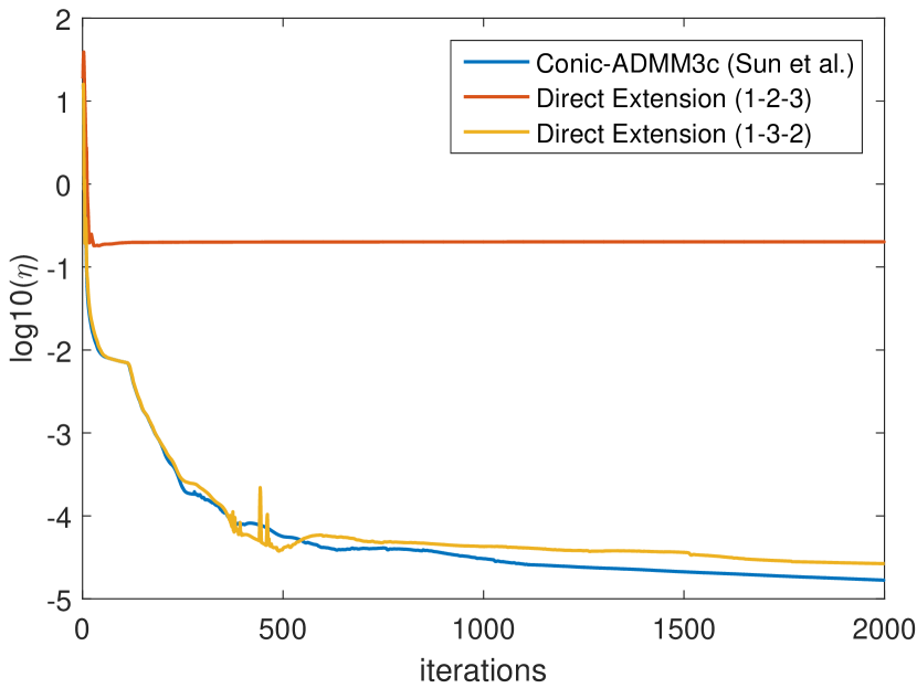
(a) Problem gr21 (TSPLIB).

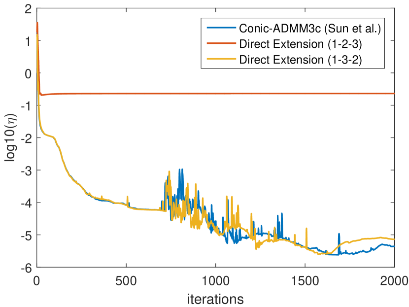
(b) Problem chr20a (QAPLIB).

Figure 2: Convergence criterion 37 as a function of the number of iterations for problems from the TSPLIB and QAPLIB for both the Conic-ADMM3c algorithm of [26] (in blue) and the direct extension of 2-block ADMM to a multi-block setting (red and yellow). Updating blocks in order 1-2-3 fails to converge. Updating in order 1-3-2 yields a convergence curve similar to the one obtained by using the algorithm in [26].

5 Results

We tested C-SDP on a variety of sparse graph matching and QAP-type problems. In particular, we used C-SDP to obtain lower and upper bounds on problems from both the QAP and TSP libraries, and to tackle the assignment problem in Nuclear Magnetic Resonance Spectroscopy (NMR).

5.1 QAP and TSP bounds

SDP relaxations like the one in [31] and C-SDP can yield both a lower bound and an upper bound for QAP-type problems. The latter is given by the objective value of the semidefinite program, while the former is obtained from $\text{Tr}\left(P^{T}APB^{T}\right)$ after projecting the doubly-stochastic matrix to the set of permutations. In what follows we present both lower and upper bounds for various QAP and TSP problems.

We compare our results against two other methods: the eigenspace relaxation [16], [17], and the convex-concave approach, PATH [30]. To the best of our knowledge, the eigenspace relaxation is the only SDP relaxation for the QAP which can handle larger graphs, although an interior point approach is slow for graphs with more than $50$ nodes. In particular, we compare our lower bounds to the ones produced by this relaxation. Although the eigenspace relaxation also produces a doubly-stochastic matrix, there is no obvious way of recovering the original permutation matrix from this variable (direct projection to the set of permutation matrices, or a Birkhoff-von Neuman decomposition [9] of the doubly stochastic matrix did not produce meaningful results). We compare our upper bounds against PATH (which produces a permutation matrix).

For both lower and upper bounds, we compute the gap:

$$\mu=\frac{\mid v^{*}-v\mid}{v^{*}}\times 100\%$$ (38)

where $v$ is the value of the bounds obtained from the relaxation and $v^{*}$ is the optimal value for the non-convex problem. The gap can be greater than $100\%$ in the case of the upper bound.

5.1.1 QAP library problems.

Figure 3 shows lower bounds on problems in the QAP library for both C-SDP with cliques of size 4 and Eigenspace (full results are shown in table 3 in the Appendix). We see that for the ’chr’ family of problems [8] C-SDP tends to be significantly better than Eigenspace. However, for the ’esc’ problem family [12], the results are divided. Eigenspace performs better than C-SDP in 10 of these problems. In 7 of these, the adjacency matrix, $B$, has more than 20% non-zero entries. This illustrates a general observed trend, where C-SDP performs best in problems with very sparse $B$.

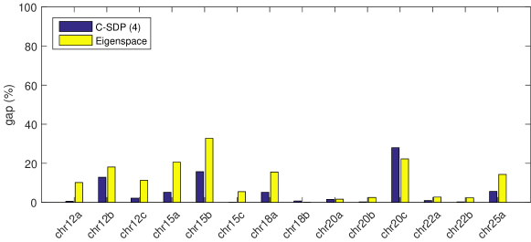
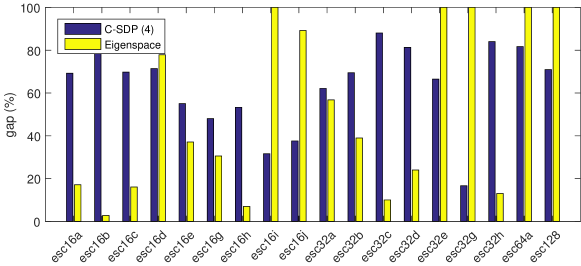
Figure 3: Lower bounds for selected problems in the QAP library. Lower bounds from C-SDP with 4 nodes per variable (blue) and for Eigenspace (yellow) are shown. C-SDP generally shows a smaller gap than Eigenspace for the ’chr’ problem family. For the ’esc’ problem family, the results are mixed. However, note that out of the 10 problems in which C-SDP underperforms, 7 of these have $B$ with more than 20% non-zero entries.

Figure 4 shows upper bounds on the same problems (full results shown in Table 4). This time, a comparison is made with the convex-concave approach, PATH. Generally, we observe that C-SDP produces strong lower bounds on these QAP problems (mostly within 20% of the optimum). Remarkably, C-SDP achieves the optimum in 7 of the problems. PATH outperforms C-SDP in terms of upper bounds in only 6 of the 32 problems.

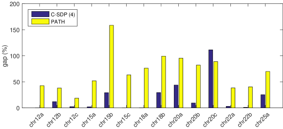
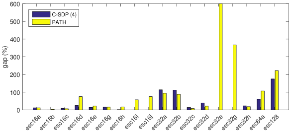
Figure 4: Upper bounds for selected problems in the QAP library. Upper bounds from C-SDP with 4 nodes per variable (blue) and for PATH (yellow) are shown. C-SDP generally shows a smaller gap than PATH.

5.1.2 TSP library problems.

Figures 5 and 6 show lower and upper bounds for problems in the TSP library. Again, we verify that C-SDP tends to produce strong lower bounds. Both C-SDP and PATH fail at producing good upper bounds on this class of problems. Tables 5 and 6 show the detailed results for lower and upper bounds, respectively.

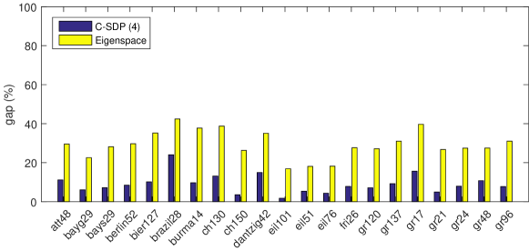
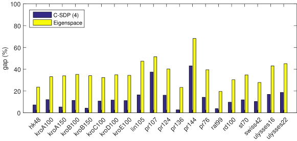
Figure 5: Lower bounds for selected problems from the TSP library ($n\leq 150$). Lower bounds from C-SDP with 4 nodes per variable (blue) and for Eigenspace (yellow) are shown. C-SDP consistently shows smaller gaps than Eigenspace, although Eigenspace can be used to quickly generate a lower bound, since it simplifies to a linear program due to the simple spectrum of B.

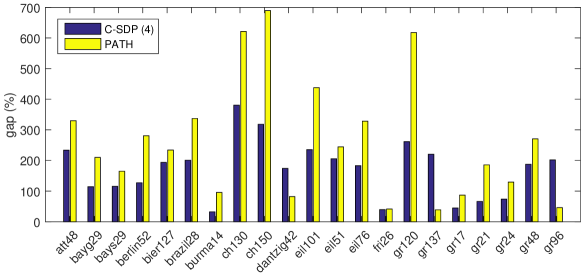
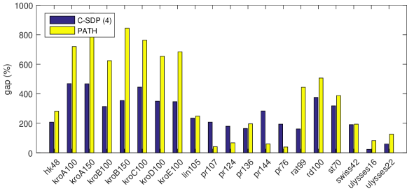
Figure 6: Upper bounds for selected problems in the TSP library ($n\leq 150$). Upper bounds from C-SDP with 4 nodes per variable (blue) and for PATH (yellow) are shown. C-SDP generally shows a smaller gap than PATH.

5.2 Application: NMR assignment

Nuclear Magnetic Resonance Spectroscopy (NMR) is the go-to tool for structural determination of proteins in solution, [29]. Structural reconstruction in NMR requires accurate geometrical constraints which are derived from the analysis of NMR spectra.

Prior to an NMR experiment, the amino acid sequence (and hence also the atomic composition of the protein) is known. In an experiment, the resonance frequencies of all atoms in the protein are simultaneously measured. In order to use the experimental measurements as constraints on the atoms, measured resonance frequencies have to be assigned to the atoms in the protein, giving rise to the resonance assignment problem. The assignment procedure is typically performed in two steps: 1) Grouping the resonance frequencies from each amino acid into spin systems; 2) Assignment of spin systems to the amino acids. One can view spin systems as a vector of resonance frequencies associated with atoms from an amino acid. By assigning each spin system to the correct amino acid, one can then infer the frequencies of the atoms that compose that amino acid.

In the following, we formulate the resonance assignment problem as a QAP (the use of the QAP for NMR assignment is not new [6], [10], although to the best of our knowledge, our formulation of the costs and constraints is novel). More precisely, when placed in the correct order, each spin system shares frequency values with its preceding neighbor, up to experimental noise, since some of the atoms of a single amino acid are featured on two adjacent spin systems. This is illustrated in Figure 7.

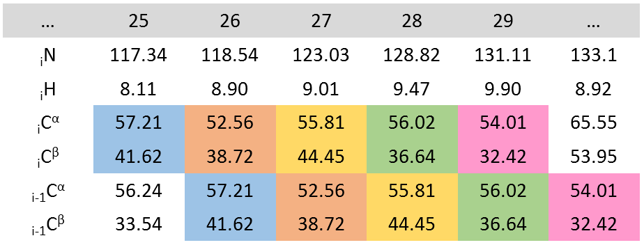
Figure 7: Example sequence of consecutive spin systems built from three NMR spectra for bmr4391 (no noise). Each spin system contains frequency information for $C^{\alpha}$ and $C^{\beta}$ in its own amino acid and the preceding amino acid.

Such a feature can be used to define a distance matrix between each pair of spin systems,

$$A_{ij}=\frac{(s_{i}(C_{i}^{\alpha})-s_{j}(C_{j-1}^{\alpha}))^{2}}{\sigma_{\alpha}^{2}}+\frac{(s_{i}(C_{i}^{\beta})-s_{j}(C_{j-1}^{\beta}))^{2}}{\sigma_{\beta}^{2}}.$$ (39)

Note that $A_{ij}$ is small if $i$ immediately precedes $j$. One wishes to find the permutation that minimizes this distance along a path of length $n-1$, which should correspond to the best ordering of the spin systems, thus allowing for their assignment to the corresponding amino acids. Alternatively, we choose instead to kernalize this distance matrix by defining

$$\bar{A}=\exp\left(-\frac{A}{||A||_{F}}\right)$$ (40)

where the exponential is applied elementwise [13]. The goal is then to maximize the kernel distance along a path of length $n-1$, amounting to the following problem

Problem 7 (NMR assignment)

$$\max_{P} \qquad\text{Tr}\left(\bar{A}PB^{T}P^{T}\right)$$

s.t. $$\qquad P\in\text{Perm}(n)$$

where $B$ is the adjacency matrix for the path graph, given by

$$B=\begin{bmatrix}0&1&\cdots&\cdots&0\\ \vdots&&\ddots&&\vdots\\ \vdots&&&&1\\ 0&\cdots&\cdots&\cdots&0\end{bmatrix}$$

This is a QAP, and the sparsity of $B$ allows the use of C-SDP to obtain a doubly stochastic matrix $D$. The matrix $D$ can in turn be projected to the set of permutation matrices to yield a valid assignment of spin systems to amino acids.

Additional information about valid assignments can be included through a term $\text{Tr}\left(W^{T}P\right)$ in the QAP cost. In particular, one verifies in practice that the resonance frequencies of the $N$, $H^{N}$, $C^{\alpha}$, and $C^{\beta}$ atoms depend strongly on the type of amino acid, as illustrated in Figure 8. Here we use a hypothesis test perspective to construct $W$. The resonance frequency distributions, conditional on the type of amino acid, were modeled as independent Normal distributions, with mean, $\mu$, and standard deviation, $\sigma$, taken from statistics collected in the Biological Magnetic Resonance Data Bank (BMRB, [27]). Let spin system $s_{i}$ be defined as the frequencies of the atoms corresponding to that spin system:

$$s_{i}=\left[\begin{array}[]{c}f_{\text{N}_{i}}\\ f_{\text{H}^{N}_{i}}\\ f_{\text{C}^{\alpha}_{i}}\\ f_{\text{C}^{\beta}_{i}}\\ f_{\text{C}^{\alpha}_{i-1}}\\ f_{\text{C}^{\beta}_{i-1}}\end{array}\right].$$ (41)

Then for spin system $s_{i}$ and amino acid $j$ one can compute

$$z_{ij}=\sum_{k=1}^{4}\frac{(s_{i}(k)-\mu_{j}(k))^{2}}{\sigma_{k}^{2}}\sim\chi^{2}_{3}$$

which follows a chi-square distribution with $3$ degrees of freedom under the distributional assumptions. The test value $z_{ij}$ can be used to determine a p-value under the null hypothesis that spin system $i$ corresponds to residue $j$. Such p-values can be used either as hard constraints on the permutation matrix $P$ (by setting $P(i,j)=0$ if $z_{ij}$ is below a set threshold) or as soft constraints by including an additional term $\text{Tr}\left(W^{T}P\right)$ in the cost where $W$ is

$$W=\exp\left(-\frac{Z}{||Z||_{F}}\right),$$

with $Z\equiv[z_{ij}]$. The latter approach is adopted in this work.

Writing the QAP in the form of Problem 1

$$\min_{Q} \qquad\text{Tr}\left(CQ\right)$$

s.t. $$\qquad Q=\text{vec}(P)\text{vec}(P)^{T}$$

$$\qquad P\in\text{Perm}(n)$$

we wish to solve this problem where $C$ is given by

$$C=-B\otimes\exp\left(-\frac{A}{||A||_{F}}\right)-\frac{1}{\gamma}\text{diag}\left(\exp\left(-\gamma\frac{Z}{||Z||_{F}}\right)\right).$$

Note that the change in the objective consisted only of adding weight terms to the diagonal, using $\gamma$ as a parameter controlling the importance of the statistical information from empirically observed frequencies. A value of $\gamma=0.1$ was used throughout all simulations.

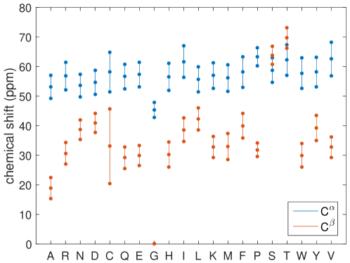
Figure 8: Chemical shift (frequency) distribution of $C^{\alpha}$ and $C^{\beta}$ atoms per residue type. The central dots correspond to the mean, and the upper and lower dots are placed two standard deviations away from the mean.

C-SDP was tested on synthetic datasets for benchmarking with cliques of size 2. The dataset was originally described in [28] and consists of a number of proteins for which spin systems are created from the existing assignments in BMRB [27]. We consider only those proteins with 100 amino acids or fewer. Each spin system is constructed by taking the assigned frequencies from the datafile for the base $N$-$H^{N}$ pair, and the $C^{\alpha}$ and $C^{\beta}$ atoms (with the exception of Glycine and Proline). The $C^{\alpha}$ and $C^{\beta}$ values from the preceding residue are then added at the end of this vector, and perturbed with additive white gaussian noise with $\sigma=(0.08,0.16)$ (low-noise) or $\sigma=(0.16,0.32)$ (high-noise).

Comparison:

We compare results with other fully automated assignment tools: MARS [14], CISA [28], and IPASS [2]. In order to compare with a different convex relaxation of the graph matching problem, we consider the doubly-stochastic relaxation (DS), in which we solve the convex problem

$$\min_{D} \qquad||AD-DB||_{F}$$

s.t. $$\qquad\text{Tr}\left(K^{T}D\right)=0$$

$$\qquad D\in\text{DS}(n)$$

where $K$ is the matrix defined by the entries

$$K(i,j)=\left\{\begin{array}[]{cl}1&\text{if }z_{ij}<\epsilon\\ 0&\text{otherwise,}\end{array}\right.$$

for some user-defined threshold $\epsilon$, thus imposing hard constraints on assignments that are statistically unlikely. The value of $\epsilon$ was progressively reduced from $\epsilon=10^{-2}$ until a satisfiable set of constraints was produced.

Evaluation:

Let $N_{m}$ be the number of spin systems assigned in the BMRB file, $N_{a}$ be the number assigned by the algorithm, and $N_{c}$ be the number of correctly assigned spin systems. We then define precision$\equiv N_{c}/N_{m}$, and recall$\equiv N_{c}/N_{a}$. These values are presented in tables 1 and 2, below.

Table 1: Accuracy of assignment (precision/recall) of various assignment packages as well as the constrained relaxed graph matching (DS) and C-SDP on synthetic spin systems with noise level = (0.08,0.16). Results for MARS [14] and CISA taken from [28]. Results for IPASS taken from [2].

Protein ID	Length	MARS	CISA	IPASS	DS	C-SDP
bmr4391	66	100/76	97/97	93/90	85.2/85.2	99.1/99.1
bmr4752	68	100/97	96/94	100/94	98.5/98.5	100/100
bmr4144	78	100/91	100/99	98/85	96.4/96.4	99.7/99.7
bmr4579	86	99/98	98/98	100/98	99.9/99.9	100/100
bmr4316	89	100/100	100/99	99/98	95.8/95.8	98.8/98.8

Table 2: Accuracy of assignment (precision/recall) of various assignment packages as well as the constrained relaxed graph matching (DS) and C-SDP on synthetic spin systems with noise level = (0.16,0.32). Results for MARS [14] and CISA taken from [28]. Results for IPASS taken from [2].

Protein ID	Length	MARS	CISA	IPASS	DS	C-SDP
bmr4391	66	100/75	91/91	93/90	85.5/85.5	100/100
bmr4752	68	100/97	90/88	100/94	87.8/87.8	99.4/99.4
bmr4144	78	100/69	100/99	98/85	85.6/85.6	96.4/96.4
bmr4579	86	96/90	80/80	100/98	89.6/89.6	99.6/99.6
bmr4316	89	99/91	83/83	99/98	95.1/95.1	97.8/97.8

C-SDP outperforms other methods in terms of both precision and recall, on average. The doubly stochastic relaxation also compares well in the low-noise scenario, but performs poorly in the high-noise setting.

Note that since C-SDP always produces a full permutation matrix, it assigns all spin systems, such that $N_{a}=N_{m}$, where $N_{m}$ is assumed to be the number of assignable spin systems in the protein. As a result, precision and recall values for C-SDP are equal. The number of spin systems may be smaller than the number of amino acids, as some amino acids such as Proline do not contribute spin systems, in which case token spin systems are used in their stead.

6 Conclusion

This work presented a new semidefinite programming (SDP) relaxation, C-SDP, for the quadratic assignment problem (QAP) in which one of the matrices is sparse. A convergent ADMM formulation was developed, which exploits the natural three-block structure of the dual problem, allowing a highly parallelizable solution where the most expensive step per iteration is a projection of a matrix of size $\mathcal{O}(n)$ to the positive semidefinite cone.

The performance of C-SDP was evaluated on problems from the QAP and TSP libraries, where we found it produces better lower bounds than comparable SDP relaxations [17] as well as competitive upper bounds (after projecting the solution to the set of permutation matrices), compared to a popular local method [30].

An application to the NMR assignment problem was also described, which can be formulated as a sparse QAP. Preliminary results on proteins from a standard synthetic dataset showed that C-SDP results in a better assignment compared to popular fully automated assignment tools in recent literature.

Appendix - Full Tabulated Results

Table 3: Comparison between lower bounds given by the C-SDP and Eigenspace relaxations on selected problems from the QAP library with (relatively) sparse B. C-SDP instances were ran for 1000 ADMM iterations on 20 processors.

Problem	Optimal	C-SDP (k=2) Gap (%)	C-SDP (k=3) Gap (%)	C-SDP (k=4) Gap (%)	Eigen- space Gap (%)
chr12a	9552	9.7	2.7	0.6	10.2
chr12b	9742	26.3	19.3	12.8	18.1
chr12c	11156	10.2	3.2	2.1	11.3
chr15a	9896	13.1	7.0	5.2	20.6
chr15b	7990	35.7	25.2	15.7	32.8
chr15c	9504	0.1	0.0	0.0	5.5
chr18a	11098	12.6	4.6	5.2	15.5
chr18b	1534	0.0	0.0	0.7	0.0
chr20a	2192	1.6	1.6	1.5	1.6
chr20b	2298	2.8	0.3	0.3	2.5
chr20c	14142	37.0	31.9	28.0	22.3
chr22a	6156	2.6	1.3	0.9	2.7
chr22b	6194	1.4	0.5	0.2	2.4
chr25a	3796	13.8	7.5	5.6	14.3
esc16a	68	100.0	80.4	69.2	17.1
esc16b	292	100.0	88.4	85.7	2.7
esc16c	160	100.0	79.4	69.8	16.1
esc16d	16	100.0	72.1	71.4	77.9
esc16e	28	100.0	78.2	55.0	37.1
esc16g	26	100.0	67.3	48.0	30.6
esc16h	996	66.3	57.0	53.3	7.0
esc16i	14	100.0	19.1	31.6	100.0
esc16j	8	100.0	53.0	37.6	89.2
esc32a	130	100.0	74.6	62.1	56.8
esc32b	168	100.0	76.1	69.5	39.0
esc32c	642	100.0	91.0	88.0	10.0
esc32d	200	100.0	88.0	81.3	24.0
esc32e	2	100.0	66.6	66.5	100.0
esc32g	6	100.0	41.0	16.7	100.0
esc32h	438	100.0	88.2	84.0	13.0
esc64a	116	99.9	86.0	81.7	-
esc128	64	99.6	75.8	71.0	-
ste36a	96772	46.9	42.1	40.2	-
ste36b	58537	70.1	67.0	65.1	-
ste36c	108159	37.7	35.2	34.2	-

Table 4: Comparison between upper bounds given by C-SDP and PATH relaxations on elected problems from the QAP library with (relatively) sparse B. C-SDP instances were ran for 1000 ADMM iterations on 20 processors.

Problem	Optimal	C-SDP (k=2) Gap (%)	C-SDP (k=3) Gap (%)	C-SDP (k=4) Gap (%)	PATH Gap (%)
chr12a	9552	34.5	6.0	0.0	42.7
chr12b	9742	38.9	25.4	11.9	38.1
chr12c	11156	5.8	2.3	2.3	18.6
chr15a	9896	2.1	2.1	2.1	52.0
chr15b	7990	26.3	34.5	29.2	158.6
chr15c	9504	0.0	0.0	0.0	63.3
chr18a	11098	69.8	0.2	0.2	76.3
chr18b	1534	8.9	22.9	29.5	99.3
chr20a	2192	122.5	76.1	43.8	95.4
chr20b	2298	62.9	9.3	9.3	82.2
chr20c	14142	173.0	100.1	111.5	88.9
chr22a	6156	17.2	7.6	3.0	38.3
chr22b	6194	7.3	2.3	1.0	40.4
chr25a	3796	107.0	49.2	25.2	69.9
esc16a	68	8.8	11.8	11.8	11.8
esc16b	292	0.0	0.7	0.0	2.7
esc16c	160	5.0	7.5	8.7	6.3
esc16d	16	12.5	50.0	25.0	75.0
esc16e	28	14.3	7.1	14.3	21.4
esc16g	26	7.7	0.0	15.4	15.4
esc16h	996	1.6	0.0	1.6	16.9
esc16i	14	0.0	0.0	0.0	57.1
esc16j	8	0.0	0.0	0.0	75.0
esc32a	130	115.4	124.6	113.8	93.8
esc32b	168	109.5	114.3	111.9	88.1
esc32c	642	12.8	15.9	13.7	7.8
esc32d	200	38.0	36.0	39.0	21.0
esc32e	2	0.0	0.0	0.0	600.0
esc32g	6	0.0	0.0	0.0	366.7
esc32h	438	24.7	26.9	22.8	18.3
esc64a	116	60.3	53.4	60.3	106.9
esc128	64	250.0	206.3	175.0	221.9
ste36a	96772	70.2	74.7	74.2	76.3
ste36b	58537	188.8	204.3	211.9	158.6
ste36c	108159	66.0	62.8	63.7	83.2

Table 5: Comparison between lower bounds given by the C-SDP and Eigenspace relaxations on problems from the TSP library (with $n\leq 150$). C-SDP instances were ran for 1000 ADMM iterations on 20 processors.

Problem	Optimal	C-SDP (k=2) Gap (%)	C-SDP (k=3) Gap (%)	C-SDP (k=4) Gap (%)	Eigen- space Gap (%)
att48	10628	20.6	10.9	11.2	29.6
bayg29	1610	10.7	6.5	6.0	22.5
bays29	2020	12.8	6.9	7.2	28.1
berlin52	7542	16.5	9.9	8.4	29.7
bier127	118282	19.5	10.4	10.1	35.2
brazil58	25395	34.6	24.1	24.0	42.4
burma14	3323	16.1	10.7	9.7	37.7
ch130	6110	26.9	12.9	13.1	38.8
ch150	6528	11.3	1.1	3.5	26.3
dantzig42	699	23.6	14.9	15.0	35.1
eil101	629	6.9	1.6	1.7	16.9
eil51	426	10.9	4.6	5.4	18.1
eil76	538	8.8	3.6	4.3	18.2
fri26	937	12.2	9.4	7.8	27.6
gr120	6942	15.1	7.1	7.1	27.2
gr137	69853	14.9	8.0	9.2	31.0
gr17	2085	21.6	20.2	15.6	39.7
gr21	2707	10.8	4.0	5.0	26.7
gr24	1272	17.3	8.7	7.9	27.4
gr48	5046	18.0	10.4	10.8	27.5
gr96	55209	15.0	8.4	7.7	31.0
hk48	11461	13.9	7.5	7.2	23.6
kroA100	21282	19.4	12.7	12.1	33.2
kroA150	26524	16.6	5.2	5.3	34.0
kroB100	22141	23.7	12.9	11.4	35.3
kroB150	26130	18.6	4.4	4.3	34.1
kroC100	20749	19.3	10.9	10.8	32.4
kroD100	21294	22.2	12.1	11.7	34.9
kroE100	22068	23.9	12.5	11.2	34.4
lin105	14379	35.2	17.3	16.5	47.4
pr107	44303	40.2	38.9	37.4	51.5
pr124	59030	25.3	14.0	16.2	40.3
pr136	96772	2.1	2.6	2.7	23.3
pr144	58537	54.7	40.7	43.1	68.2
pr76	108159	28.3	15.3	14.2	39.5
rat99	1211	10.4	2.8	3.8	19.7
rd100	7910	16.9	10.7	9.8	30.3
st70	675	22.1	13.6	11.9	34.8
swiss42	1273	20.6	10.7	10.4	27.9
ulysses16	6859	25.2	17.1	17.0	43.1
ulysses22	7013	28.5	19.7	18.7	45.2

Table 6: Comparison between upper bounds given by C-SDP and PATH relaxations on problems from the TSP library (with $n\leq 150$). C-SDP instances were ran for 1000 ADMM iterations on 20 processors.

Problem	Optimal	C-SDP (k=2) Gap (%)	C-SDP (k=3) Gap (%)	C-SDP (k=4) Gap (%)	PATH Gap (%)
att48	10628	213.0	236.5	233.6	329.8
bayg29	1610	114.3	115.8	114.3	210.1
bays29	2020	107.6	118.3	115.4	164.8
berlin52	7542	175.0	127.2	127.2	280.6
bier127	118282	216.4	193.8	193.8	234.2
brazil58	25395	248.0	200.8	200.8	337.0
burma14	3323	24.6	28.4	32.3	95.5
ch130	6110	352.4	380.6	380.6	621.3
ch150	6528	346.9	318.2	318.2	689.3
dantzig42	699	193.1	174.0	174.0	82.0
eil101	629	227.3	235.3	235.3	437.7
eil51	426	203.6	205.4	205.5	244.4
eil76	538	282.9	183.0	183.0	328.2
fri26	937	91.6	39.4	39.4	41.6
gr120	6942	445.2	261.6	261.6	617.6
gr137	69853	264.6	220.3	220.3	38.9
gr17	2085	46.8	32.4	44.9	86.9
gr21	2707	94.5	69.7	66.3	185.7
gr24	1272	89.2	86.2	73.9	129.4
gr48	5046	210.2	187.4	187.4	270.4
gr96	55209	228.9	201.7	201.7	46.0
hk48	11461	222.4	207.7	207.7	281.6
kroA100	21282	469.6	469.0	469.0	720.2
kroA150	26524	411.0	467.4	467.4	945.8
kroB100	22141	411.9	313.6	313.6	624.2
kroB150	26130	417.3	353.7	353.7	844.7
kroC100	20749	507.4	445.1	445.1	763.0
kroD100	21294	504.2	349.8	349.8	654.4
kroE100	22068	489.5	346.3	346.3	684.2
lin105	14379	303.1	234.8	234.8	248.4
pr107	44303	181.5	207.9	207.9	41.6
pr124	59030	293.8	180.2	180.2	67.6
pr136	96772	325.5	164.7	164.7	196.6
pr144	58537	255.0	283.7	283.7	59.8
pr76	108159	192.2	194.0	194.0	39.4
rat99	1211	236.4	161.5	161.5	444.1
rd100	7910	438.4	375.3	375.3	506.5
st70	675	300.9	320.0	317.9	387.9
swiss42	1273	163.2	190.4	190.8	194.0
ulysses16	6859	23.6	20.2	23.2	82.7
ulysses22	7013	64.5	57.0	59.7	126.3

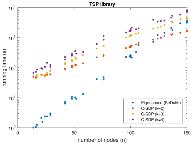
Figure 9: Comparison of run times between C-SDP and Eigenspace (linear program) relexations on problems from the TSP library (with $n\leq 150$). C-SDP instances were ran for 1000 ADMM iterations on 20 processors. Eigenspace instances were solved using SeDuMi [25]. As the Eigenspace relaxation simplifies to a linear program in the case of TSP, solving the problem using an interior point solver is stil competitive with the ADMM approach used in C-SDP.

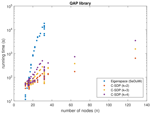
Figure 10: Comparison of run times between C-SDP and Eigenspace relexations on problems from the QAP library (with $n\leq 150$). C-SDP instances were ran for 1000 ADMM iterations on 20 processors. Eigenspace instances were solved using SeDuMi [25]. In the case of problems from the QAP library, the Eigenspace relaxation no longer simplifies, resulting in longer runtimes.

References

- [1] Aflalo, Y., Bronstein, A., Kimmel, R.: On convex relaxation of graph isomorphism. Proceedings of the National Academy of Sciences 112(10), 2942–2947 (2015). DOI 10.1073/pnas.1401651112. URL http://www.pnas.org/content/112/10/2942.abstract
- [2] Alipanahi, B., Gao, X., Karakoc, E., Li, S., Balbach, F., Feng, G., Donaldson, L., Li, M.: Error tolerant nmr backbone resonance assignment and automated structure generation. Journal of Biomolecular NMR 9(1), 15–41 (2011)
- [3] Almohamad, H., Duffuaa, S.O.: A linear programming approach for the weighted graph matching problem. IEEE Transactions on pattern analysis and machine intelligence 15(5), 522–525 (1993)
- [4] Babai, L.: Graph Isomorphism in Quasipolynomial Time. ArXiv e-prints (2015)
- [5] Burkard, R.E., Karisch, S.E., Rendl, F.: Qaplib – a quadratic assignment problemlibrary. J. of Global Optimization 10(4), 391–403 (1997). DOI 10.1023/A:1008293323270. URL http://dx.doi.org/10.1023/A:1008293323270
- [6] Cavuslar, G., Catay, B., Apaydin, M.S.: A tabu search approach for the nmr protein structure-based assignment problem. IEEE/ACM Trans. Comput. Biol. Bioinformatics 9(6), 1621–1628 (2012). DOI 10.1109/TCBB.2012.122. URL http://dx.doi.org/10.1109/TCBB.2012.122
- [7] Chen, C., He, B., Ye, Y., Yuan, X.: The direct extension of admm for multi-block convex minimization problems is not necessarily convergent. Math. Program. 155(1-2), 57–79 (2016). DOI 10.1007/s10107-014-0826-5. URL http://dx.doi.org/10.1007/s10107-014-0826-5
- [8] Christofides, N., Benavent, E.: An exact algorithm for the quadratic assignment problem on a tree. Operations Research 37(5), pp. 760–768 (1989). URL http://www.jstor.org/stable/171021
- [9] Dufossé, F., Uçar, B.: Notes on birkhoff–von neumann decomposition of doubly stochastic matrices. Linear Algebra and its Applications 497, 108 – 115 (2016). DOI http://dx.doi.org/10.1016/j.laa.2016.02.023. URL http://www.sciencedirect.com/science/article/pii/S0024379516001257
- [10] Eghbalnia, H.R., Bahrami, A., Wang, L., Assadi, A., Markley, J.L.: Probabilistic identification of spin systems and their assignments including coil–helix inference as output (pistachio). Journal of Biomolecular NMR 32(3), 219–233 (2005). DOI 10.1007/s10858-005-7944-6. URL http://dx.doi.org/10.1007/s10858-005-7944-6
- [11] Elias Oliveira, D., Wolkowicz, H., Xu, Y.: ADMM for the SDP relaxation of the QAP. ArXiv e-prints (2015)
- [12] Eschermann, B., Wunderlich, H.J.: Optimized synthesis of self-testable finite state machines. In: Fault-Tolerant Computing, 1990. FTCS-20. Digest of Papers., 20th International Symposium, pp. 390–397 (1990). DOI 10.1109/FTCS.1990.89393
- [13] Genton, M.G.: Classes of kernels for machine learning: A statistics perspective. J. Mach. Learn. Res. 2, 299–312 (2002). URL http://dl.acm.org/citation.cfm?id=944790.944815
- [14] Jung, Y.S., Zweckstetter, M.: Mars - robust automatic backbone assignment of proteins. Journal of Biomolecular NMR 30(1), 11–23 (2004). DOI 10.1023/B:JNMR.0000042954.99056.ad. URL http://dx.doi.org/10.1023/B%3AJNMR.0000042954.99056.ad
- [15] Kezurer, I., Kovalsky, S.Z., Basri, R., Lipman, Y.: Tight Relaxation of Quadratic Matching. Computer Graphics Forum (2015). DOI 10.1111/cgf.12701
- [16] de Klerk, E., Sotirov, R.: Exploiting group symmetry in semidefinite programming relaxations of the quadratic assignment problem. Mathematical Programming 122(2), 225–246 (2010). DOI 10.1007/s10107-008-0246-5. URL http://dx.doi.org/10.1007/s10107-008-0246-5
- [17] de Klerk, E., Sotirov, R., Truetsch, U.: A new semidefinite programming relaxation for the quadratic assignment problem and its computational perspectives. INFORMS Journal on Computing 27(2), 378–391 (2015). DOI 10.1287/ijoc.2014.0634. URL http://dx.doi.org/10.1287/ijoc.2014.0634
- [18] Koopmans, T., Beckmann, M.J.: Assignment problems and the location of economic activities. Cowles Foundation Discussion Papers 4, Cowles Foundation for Research in Economics, Yale University (1955). URL http://EconPapers.repec.org/RePEc:cwl:cwldpp:4
- [19] Loiola, E.M., de Abreu, N.M.M., Boaventura-Netto, P.O., Hahn, P., Querido, T.: A survey for the quadratic assignment problem. European Journal of Operational Research 176(2), 657 – 690 (2007). DOI http://dx.doi.org/10.1016/j.ejor.2005.09.032. URL http://www.sciencedirect.com/science/article/pii/S0377221705008337
- [20] Lyzinski, V., Fishkind, D.E., Fiori, M., Vogelstein, J.T., Priebe, C.E., Sapiro, G.: Graph Matching: Relax at Your Own Risk. IEEE Transactions on Pattern Analysis and Machine Intelligence 38(1) (2016)
- [21] Peng, J., Mittelmann, H., Li, X.: A new relaxation framework for quadratic assignment problems based on matrix splitting. Mathematical Programming Computation 2(1), 59–77 (2010). DOI 10.1007/s12532-010-0012-6. URL http://dx.doi.org/10.1007/s12532-010-0012-6
- [22] Peng, J., Zhu, T., Luo, H., Toh, K.C.: Semi-definite programming relaxation of quadratic assignment problems based on nonredundant matrix splitting. Computational Optimization and Applications 60(1), 171–198 (2015). DOI 10.1007/s10589-014-9663-y. URL http://dx.doi.org/10.1007/s10589-014-9663-y
- [23] Ramana, M.V., Scheinerman, E.R., Ullman, D.: Fractional isomorphism of graphs. Discrete Mathematics 132(1-3), 247–265 (1994)
- [24] Sahni, S., Gonzalez, T.: P-complete approximation problems. J. ACM 23(3), 555–565 (1976). DOI 10.1145/321958.321975. URL http://doi.acm.org/10.1145/321958.321975
- [25] Sturm, J.F.: Using sedumi 1.02, a matlab toolbox for optimization over symmetric cones. Optimization Methods and Software 11(1-4), 625–653 (1999). DOI 10.1080/10556789908805766. URL http://dx.doi.org/10.1080/10556789908805766
- [26] Sun, D., Toh, K.C., Yang, L.: A convergent 3-block semiproximal alternating direction method of multipliers for conic programming with 4-type constraints. SIAM Journal on Optimization 25(2), 882–915 (2015). DOI 10.1137/140964357. URL http://dx.doi.org/10.1137/140964357
- [27] Ulrich, E.L., Akutsu, H., Doreleijers, J.F., Harano, Y., Ioannidis, Y.E., Lin, J., Livny, M., Mading, S., Maziuk, D., Miller, Z., Nakatani, E., Schulte, C.F., Tolmie, D.E., Kent Wenger, R., Yao, H., Markley, J.L.: Biomagresbank. Nucleic Acids Research 36(suppl 1), D402–D408 (2008). DOI 10.1093/nar/gkm957. URL http://nar.oxfordjournals.org/content/36/suppl_1/D402.abstract
- [28] Wan, X., Lin, G.: Cisa: Combined nmr resonance connectivity information determination and sequential assignment. Computational Biology and Bioinformatics, IEEE/ACM Transactions on 4(3), 336–348 (2007). DOI 10.1109/tcbb.2007.1047
- [29] Wuthrich, K., Wider, G., Wagner, G., Braun, W.: Sequential resonance assignments as a basis for determination of spatial protein structures by high resolution proton nuclear magnetic resonance. Journal of Molecular Biology 155(3), 311 – 319 (1982). DOI http://dx.doi.org/10.1016/0022-2836(82)90007-9. URL http://www.sciencedirect.com/science/article/pii/0022283682900079
- [30] Zaslavskiy, M., Bach, F., Vert, J.P.: A path following algorithm for the graph matching problem. Pattern Analysis and Machine Intelligence, IEEE Transactions on 31(12), 2227–2242 (2009). DOI 10.1109/TPAMI.2008.245
- [31] Zhao, Q., Karisch, S., Rendl, F., Wolkowicz, H.: Semidefinite programming relaxations for the quadratic assignment problem. Journal of Combinatorial Optimization 2(1), 71–109 (1998). DOI 10.1023/A:1009795911987. URL http://dx.doi.org/10.1023/A%3A1009795911987