Protection of Entanglement in the presence of Markovian or Non-Markovian Environment via particle velocity : Exact Results

Abstract

On the analytic ground we examine a physical mechanism how particle velocity can protect an entanglement when quantum system is embedded in Markovian or non-Markovian environment. In particular the effect of particle velocity is examined in the entanglement sudden death (ESD) and revival of entanglement (ROE) phenomena. Even though particles move fast, the ESD phenomenon does not disappear if it occurs at zero velocity. However the time domain $0\leq t\leq t_{*}$ for nonvanishing entanglement becomes larger and larger with increasing velocity. When ROE phenomenon occurs at zero velocity, even small velocity can make this phenomenon not to occur although the oscillatory behavior of entanglement in time is maintained. For comparatively large velocity the amplitude of the oscillatory behavior becomes extremely small. In this way the entanglement can be protected by particle velocity. The protection of entanglement via velocity is compared with that via the detuning parameter.

Quantum entanglementhorodecki09 is the most important physical resource for development of quantum technology. As shown for last two decades it plays a crucial role in quantum teleportationteleportation , superdense codingsuperdense , quantum cloningclon , and quantum cryptographycryptography . It is also quantum entanglement, which makes the quantum computer outperform the classical onetext ; computer .

Since quantum entanglement is purely quantum property, it can be maintained in time only in ideally isolated system. However, real physical systems inevitably interact with their surroundings. Thus, physical system loses its entanglement by contacting the environment. In this reason we expect that the degradation of entanglement occursyu02-1 ; simon02-1 ; dur04-1 .

Usually, the degradation of entanglement emerges as a form of an exponential decay in time by successive halves. For particular initial states, however, the entanglement sudden death (ESD) occurs when the entangled multipartite quantum system is embedded in Markovian environmentsmarkovian ; yu05-1 ; yu06-1 ; yu09-1 . This means that the entanglement is completely disentangled at finite times. This ESD phenomenon has been revealed experimentallyalmeida07 ; laurat07 .

The dynamics of entanglement was also examined when the physical system is embedded in non-Markovian environmentbreuer02 ; bellomo07 . It has been shown that there is a revival of entanglement (ROE) after a finite period of time of its complete disappearance. This is mainly due to the memory effect of the non-Markovian environment. This ROE phenomenon was shown in Ref.bellomo07 by making use of the two qubit system and concurrenceconcurrence1 as a bipartite entanglement measure. Subsequently, many works have been done to quantify the non-Markovianitybreuer09 ; vacchini11 ; chruscinski11 ; rivas14 ; hall14 ; kwang15-1 ; park16 .

The degradation of entanglement is a crucial obstacle in real quantum information processing. In order to overcome this problem we should reduce the effect of decoherence as much as possible. For this purpose various techniques were developed for Markovianprotection1 and non-Markovianprotection2 environments. Recently, it was shown that the protection of entanglement is possible by increasing the particle velocity when the quantum system is embedded in the non-Markovian environmentvelocity . The authors in Ref.velocity examined the effect of velocity by applying the fourth-order Runge-Kutta numerical method. However, it is in general difficult to understand the physical mechanism exactly from a numerical technique. In order to understand how the particle velocity reduces the effect of decoherence we need to reconsider this issue on the analytic ground, which is main motivation of present paper. There is another minor motivation. The authors of Ref.velocity argued that the dynamics of entanglement is not dependent on the particle velocity and the transition frequency individually, but depends on their multiplication. However, we cannot find any physical reason for this dependence. Our analytic approach shows that this argument is not true, but is approximately true for some cases. Thus, we examine again the effect of particle velocity in the presence of Markovian or non-Markovian environment analytically. In particular, we examine in detail how the ESD and ROE phenomena are affected by particle velocity.

We choose exactly the same physical setup with that of Ref.velocity , that is, the whole system is composed of two non-interacting identical systems. Each subsystem consists of an atom qubit and a structured environment made of two perfect reflecting mirrors at the positions $z=-L$ and $z=\ell$ with a partially reflecting mirror at $z=0$. The electromagnetic fields inside the cavities plays a role of environment.

We will briefly describe how the entanglement dynamics can be derived schematically. The detailed derivation is in Ref.velocity . The dynamics of one atom and its environment is governed by the Schrödinger equation $\frac{d}{dt}\psi(t)=-iH_{I}(t)\psi(t)$, where $H_{I}$ is a Hamiltonian for single atom and its interaction with an environment. Solving this Schrödinger equation with appropriate boundary conditions arising in the cavities, one can derive the state $\rho(t)$ of single atom by taking a partial trace with respect to its environment, that is, $\rho(t)=\mbox{tr}_{env}\lvert\psi(t)\rangle\langle\psi(t)\lvert$. Since two atoms interacts only and independently with its own environment, the quantum state of two atoms can be derived by the Kraus operatorskraus83 . For example, if the initial state of two atoms is

$$\lvert\Psi\rangle=a\lvert 00\rangle+b\lvert 11\rangle$$ (1)

where $a$ is real and positive, and $b=|b|e^{i\delta}$ with $a^{2}+|b|^{2}=1$, the concurrence at time $t$ is given by

$${\cal C}(t)=\max\bigg{[}0,2|b||P(t)|^{2}\big{(}a-|b|[1-|P(t)|^{2}]\big{)}\bigg{]},$$ (2)

where $P(t)$ satisfies the integral equation

$$\frac{d}{dt}P(t)=-\int_{0}^{t}dsf(t,s)P(s).$$ (3)

If velocity of atom is $v$ and its transition frequency is $\omega_{0}$, the correlation function $f(t,s)$ is given by

$$f(t,s)=\int_{\infty}^{\infty}d\omega J(\omega)\sin\left[\omega(\beta t-\tau)\right]\sin\left[\omega(\beta s-\tau)\right]e^{-i(\omega-\omega_{0})(t-s)}$$ (4)

where $\beta=v/c$, $\tau=\ell/c$, and the spectral densitybreuer02 is

$$J(\omega)=\frac{1}{2\pi}\frac{\gamma_{0}\lambda^{2}}{(\omega_{0}-\omega-\Delta)^{2}+\lambda^{2}}.$$ (5)

In order to neglect the relativistic effect we should require $\beta<<1$. In equation (4) the sine terms in integral comes from boundary conditions at the mirrors. In Eq. (5) the parameter $\lambda$ defines the spectral width of the coupling, which is connected to the reservoir correlation time $\tau_{B}$ by the relation $\tau_{B}\approx 1/\lambda$ and the relaxation time scale $\tau_{R}$ on which the state of the system changes is related to $\gamma_{0}$ by $\tau_{R}\approx 1/\gamma_{0}$. The parameter $\Delta$ is a detuning parameter. Thus, the center frequency of the cavity is detuned by an amount $\Delta$ against the atomic transition frequency $\omega_{0}$.

Now, we want to compute $P(t)$ analytically as much as possible. Inserting Eq. (5) into Eq. (4) $f(t,s)$ can be written as

$$f(t,s)=-\frac{\gamma_{0}\lambda^{2}}{8\pi}\sum_{j=1}^{4}f_{j}(t,s)$$ (6)

where

$$f_{1}(t,s)=\exp\bigg{[}i(\omega_{0}-\Delta)\left\{\beta(t+s)-2\tau\right\}+i\Delta(t-s)\bigg{]}\int_{-\infty}^{\infty}du\frac{e^{-iu[(1-\beta)t-(1+\beta)s+2\tau]}}{u^{2}+\lambda^{2}}$$

$$f_{2}(t,s)=\exp\bigg{[}-i(\omega_{0}-\Delta)\left\{\beta(t+s)-2\tau\right\}+i\Delta(t-s)\bigg{]}\int_{-\infty}^{\infty}du\frac{e^{-iu[(1+\beta)t-(1-\beta)s-2\tau]}}{u^{2}+\lambda^{2}}$$

$$f_{3}(t,s)=-e^{i(t-s)[\beta\omega_{0}+(1-\beta)\Delta]}\int_{-\infty}^{\infty}du\frac{e^{-iu(1-\beta)(t-s)}}{u^{2}+\lambda^{2}}$$ (7)

$$f_{4}(t,s)=-e^{i(t-s)[-\beta\omega_{0}+(1+\beta)\Delta]}\int_{-\infty}^{\infty}du\frac{e^{-iu(1+\beta)(t-s)}}{u^{2}+\lambda^{2}}.$$

Making use of

$$\int_{-\infty}^{\infty}\frac{e^{-iau}}{u^{2}+\lambda^{2}}du=\frac{\pi}{\lambda}e^{-\lambda|a|},$$ (8)

the correlation function $f(t,s)$ in Eq. (6) reduces to

$$f(t,s)=\frac{\gamma_{0}\lambda}{8}\Bigg{[}e^{i[\beta\omega_{0}+(1-\beta)\Delta](t-s)}e^{-\lambda(1-\beta)|t-s|}+e^{i[-\beta\omega_{0}+(1+\beta)\Delta](t-s)}e^{-\lambda(1+\beta)|t-s|}$$ (9)

$$\hskip 51.21504pt-\exp\bigg{\{}i(\omega_{0}-\Delta)[\beta(t+s)-2\tau]+i\Delta(t-s)\bigg{\}}e^{-\lambda|(1-\beta)t-(1+\beta)s+2\tau|}$$

$$\hskip 51.21504pt-\exp\bigg{\{}-i(\omega_{0}-\Delta)[\beta(t+s)-2\tau]+i\Delta(t-s)\bigg{\}}e^{-\lambda|(1+\beta)t-(1-\beta)s-2\tau|}\Bigg{]}.$$

In the continuum limit ($\tau\rightarrow\infty$) Eq. (9) is simplified as

$$f(t,s)=\frac{\gamma_{0}\lambda}{8}\Bigg{[}e^{i[\beta\omega_{0}+(1-\beta)\Delta](t-s)-\lambda(1-\beta)|t-s|}+e^{i[-\beta\omega_{0}+(1+\beta)\Delta](t-s)-\lambda(1+\beta)|t-s|}\Bigg{]}.$$ (10)

When $t>s$, it is more simplifies in a form

$$f(t,s)=g(t-s)$$ (11)

where

$$g(t)=\frac{\gamma_{0}\lambda}{4}\cosh(\alpha t)e^{-\bar{\lambda}t}$$ (12)

with $\bar{\lambda}=\lambda-i\Delta$ and $\alpha=\beta(\bar{\lambda}+i\omega_{0})$. Thus Eq. (3) simply reduces to

$$\frac{d}{dt}P(t)=-(g*P)(t)$$ (13)

where $*$ means a convolution.

In order to derive $P(t)$ explicitly we take a Laplace transform $\hat{f}(p)\equiv\int_{0}^{\infty}f(t)e^{-pt}dt$ to both sides of Eq. (13). Using $P(t=0)=1$ one can show easily

$$\hat{P}(p)=\frac{1}{p+\hat{g}(p)}.$$ (14)

From Eq. (12) it is also easy to show

$$\hat{g}(p)=\frac{\gamma_{0}\lambda}{8}\left(\frac{1}{p+v_{+}}+\frac{1}{p+v_{-}}\right)$$ (15)

where $v_{\pm}\equiv\bar{\lambda}\pm\alpha$. Inserting Eq. (15) into Eq. (14) one can show directly

$$\hat{P}(p)=\frac{(p+v_{+})(p+v_{-})}{(p-p_{1})(p-p_{2})(p-p_{3})}$$ (16)

where $p_{j}\hskip 5.69046pt(j=1,2,3)$ are roots of

$$p^{3}+2\bar{\lambda}p^{2}+\left(v_{+}v_{-}+\frac{\gamma_{0}\lambda}{4}\right)p+\frac{\gamma_{0}\lambda\bar{\lambda}}{4}=0.$$ (17)

Since general cubic equation can be solved analytically, it is always possible to obtain the analytical expressions of $p_{j}$ even though their expressions are too lengthy except few special cases.

The inverse Laplace transform of Eq. (16) can be easily performed by applying the Bromwich integral formula in complex plane, i.e.

$$P(t)=\mbox{sum of residues of }\hat{P}(z)e^{zt}.$$ (18)

Thus $P(t)$ becomes

$$P(t)=\frac{(p_{1}+v_{+})(p_{1}+v_{-})}{(p_{1}-p_{2})(p_{1}-p_{3})}e^{p_{1}t}-\frac{(p_{2}+v_{+})(p_{2}+v_{-})}{(p_{1}-p_{2})(p_{2}-p_{3})}e^{p_{2}t}+\frac{(p_{3}+v_{+})(p_{3}+v_{-})}{(p_{1}-p_{3})(p_{2}-p_{3})}e^{p_{3}t}.$$ (19)

In real calculation it is convenient to introduce following dimensionless parameters

$$x_{1}=\frac{\lambda}{\gamma_{0}}\hskip 28.45274ptx_{2}=\frac{\omega_{0}}{\gamma_{0}}\hskip 28.45274ptx_{3}=\frac{\Delta}{\gamma_{0}}\hskip 28.45274ptx=\gamma_{0}t.$$ (20)

Now we define $q\equiv p/\gamma_{0}$. Then the cubic equation Eq. (17) reduces to

$$q^{3}+2(x_{1}-ix_{3})q^{2}+\left(u_{+}u_{-}+\frac{x_{1}}{4}\right)q+\frac{x_{1}(x_{1}-ix_{3})}{4}=0$$ (21)

where

$$u_{\pm}\equiv\frac{v_{\pm}}{\gamma_{0}}=(1\pm\beta)x_{1}\pm i\beta x_{2}-i(1\pm\beta)x_{3}.$$ (22)

If $q_{j}\hskip 5.69046pt(j=1,2,3)$ are roots of Eq. (21), $P(t)$ can be expressed as

$$P(t)=\frac{(q_{1}+u_{+})(q_{1}+u_{-})}{(q_{1}-q_{2})(q_{1}-q_{3})}e^{q_{1}x}-\frac{(q_{2}+u_{+})(q_{2}+u_{-})}{(q_{1}-q_{2})(q_{2}-q_{3})}e^{q_{2}x}+\frac{(q_{3}+u_{+})(q_{3}+u_{-})}{(q_{1}-q_{3})(q_{2}-q_{3})}e^{q_{3}x}.$$ (23)

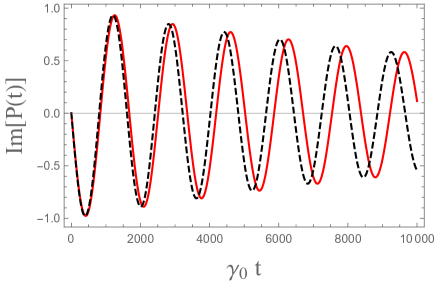
Figure 1: (Color online) The $\gamma_{0}t$-dependence of Im$[P(t)]$ when $\lambda=1.5\gamma_{0}$ and $\Delta=100\gamma_{0}$. The red solid and black dashed lines correspond to ($\beta=0.01$, $\omega_{0}=10\gamma_{0}$) and ($\beta=0.2$, $\omega_{0}=0.5\gamma_{0}$) respectively. The discrepancy of these two lines implies that the dynamics of entanglement depends on $\beta$ and $\omega_{0}$ individually.

As commented earlier authors in Ref.velocity claimed that the dynamics of entanglement is not dependent on $\beta$ and $\omega_{0}$ individually, but depends on $\beta\omega_{0}$. However, this is not correct statement. The cubic equation (21) depends on $\beta$ and $x_{2}$ only through $u_{\pm}$. Since $\beta<<1$, $u_{\pm}$ can be written approximately as $u_{\pm}\approx(x_{1}-ix_{3})\pm i\beta x_{2}$ provided that $x_{2}$ is comparatively larger than $x_{1}$ and $x_{3}$. In this case the statement of Ref.velocity is right approximately. For other cases the dynamics of entanglement depends on $\beta$ and $\omega_{0}$ individually. In order to show this explicitly we plot the $\gamma_{0}t$-dependence of Im$[P(t)]$ in Fig. 1. The red solid line corresponds to $\beta=0.01$ and $\omega_{0}=10\gamma_{0}$, and black dashed line is for $\beta=0.2$ and $\omega_{0}=0.5\gamma_{0}$. Other parameters are chosen as $\lambda=1.5\gamma_{0}$ and $\Delta=100\gamma_{0}$. The discrepancy of these two lines implies that the dynamics of entanglement is dependent on $\beta$ and $\omega_{0}$ individually.

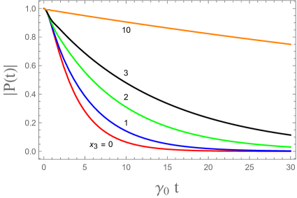
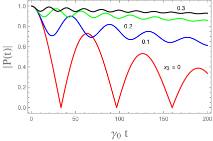
Figure 2: (Color online) Plot of $|P(t)|$ when $\beta=0$. We choose Markovian ($x_{1}=2$) in (a) and non-Markovian ($x_{1}=0.01$) regimes in (b) respectively with varying $\Delta$. As these figures show, the effect of decoherence is diminished with increasing $\Delta$.

Now, we consider few special cases. First let us consider the stationary case ($\beta=0$). In this case $u_{+}$ and $u_{-}$ are identical as $u_{+}=u_{-}\equiv u=x_{1}-ix_{3}$. Furthermore, the roots of Eq. (21) are simply

$$q_{1}=-u\hskip 14.22636ptq_{2}=-\frac{1}{2}\left(u-\sqrt{u^{2}-x_{1}}\right)\hskip 14.22636ptq_{3}=-\frac{1}{2}\left(u+\sqrt{u^{2}-x_{1}}\right).$$ (24)

Then, it is simple to derive $P(t)$ in a form

$$P(t)=e^{-\frac{\lambda-i\Delta}{2}t}\left[\cosh\left(\frac{\sqrt{(\lambda-i\Delta)^{2}-\gamma_{0}\lambda}}{2}t\right)+\frac{\lambda-i\Delta}{\sqrt{(\lambda-i\Delta)^{2}-\gamma_{0}\lambda}}\sinh\left(\frac{\sqrt{(\lambda-i\Delta)^{2}-\gamma_{0}\lambda}}{2}t\right)\right].$$ (25)

If $\Delta=0$, Eq. (25) reproduces the well-known expressions, that is

$$P(t)=e^{-\lambda t/2}\left[\cosh\left(\frac{\bar{d}}{2}t\right)+\frac{\lambda}{\bar{d}}\sinh\left(\frac{\bar{d}}{2}t\right)\right]$$ (26)

in the weak coupling regime $\lambda>\gamma_{0}$ and

$$P(t)=e^{-\lambda t/2}\left[\cos\left(\frac{d}{2}t\right)+\frac{\lambda}{d}\sin\left(\frac{d}{2}t\right)\right]$$ (27)

in strong coupling regime $\lambda<\gamma_{0}$, where $\bar{d}=\sqrt{\lambda^{2}-\gamma_{0}\lambda}$ and $d=\sqrt{\gamma_{0}\lambda-\lambda^{2}}$. Eq. (26) and Eq. (27) are responsible for the decoherence of Markovian and non-Markovian environments. When $\Delta\neq 0$, $P(t)$ in Eq. (25) is a complex quantity. In order to explore the effect of $\Delta$ we plot $|P(t)|$ for $\beta=0$ in Fig.2 with choosing $\lambda=2\gamma_{0}$ in Fig. 2(a) and $\lambda=0.01\gamma_{0}$ in Fig. 2(b). We also choose various $\Delta$ in each figure. As Fig. 2 exhibits, the effect of Markovian and non-Markovian environments is diminished with increasing $\Delta$. In this way one can protect the entanglement by making use of the detuning parameter $\Delta$protection2 too. These figures show that non-Markovian environment is more sensitive to $\Delta$ than Markovian environment.

Another special case we consider is a slow moving case ($\beta\rightarrow 0$). In this case the roots of the cubic equation (21) can be obtained perturbatively as follows;

$$q_{1}=-u+\delta q_{1}\beta^{2}+{\cal O}(\beta^{4})\hskip 28.45274ptq_{2}=-\frac{1}{2}(u-\sqrt{u^{2}-x_{1}})+\delta q_{2}\beta^{2}+{\cal O}(\beta^{4})$$ (28)

$$\hskip 99.58464ptq_{3}=-\frac{1}{2}(u+\sqrt{u^{2}-x_{1}})+\delta q_{3}\beta^{2}+{\cal O}(\beta^{4})$$

where

$$\delta q_{1}=-\frac{4u(u+ix_{2})^{2}}{x_{1}}\hskip 28.45274pt\delta q_{2}=-\frac{(u+ix_{2})^{2}}{x_{1}\sqrt{u^{2}-x_{1}}}\left(u-\sqrt{u^{2}-x_{1}}\right)^{2}$$ (29)

$$\hskip 71.13188pt\delta q_{3}=\frac{(u+ix_{2})^{2}}{x_{1}\sqrt{u^{2}-x_{1}}}\left(u+\sqrt{u^{2}-x_{1}}\right)^{2}.$$

Inserting Eq. (28) into Eq. (23) one can derive $P(t)$ analytically up to order of $\beta^{2}$.

Now, let us examine the dynamics of entanglement in the presence of Markovian or non-Markovian environment when the initial state is $\lvert\Psi\rangle$ in Eq. (1). Thus the bipartite entanglement at time $t$ is given by Eq. (2). It is known that the entanglement is protected by not only $\Delta$ but also $\beta$ independently. We will examine how ESD and ROE phenomena are affected by $\beta$ or $\Delta$.

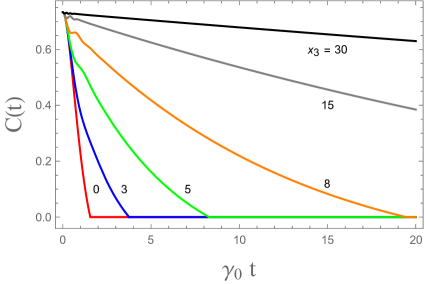
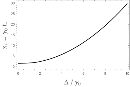
Figure 3: (Color online) (a) Plot of ${\cal C}(t)$ with choosing $x_{3}=0,3,5,8,15,30$ when other parameters are fixed as $a=0.4$, $\lambda=2\gamma_{0}$, and $\beta=\omega_{0}=0$. The time domain $0\leq x\leq x_{*}\equiv\gamma_{0}t_{*}$ for nonvanishing entanglement becomes larger and larger with increasing $\Delta$. (b) Plot of $x_{3}$-dependence of $x_{*}$ when same values of other parameters are chosen. As expected, $x_{*}$ increases with increasing $x_{3}$ quadratically. (see Eq. (30))

In Fig. 3 we examine the effect of the detuning parameter $\Delta$ in the ESD phenomenon in the Markovian regime. In Fig. 3(a) we plot $\gamma_{0}t$-dependence of ${\cal C}(t)$ with varying $\Delta$ when other parameters are fixed as $a=0.4$, $\lambda=2\gamma_{0}$, and $\beta=\omega_{0}=0$. As this figure exhibits, the ESD phenomenon occurs regardless of $\Delta$. However, the time domain $0\leq x\leq x_{*}\equiv\gamma_{0}t_{*}$, where the entanglement is nonvanishing, becomes larger with increasing $\Delta$. In this way the entanglement is protected even in the Markovian environment with increasing the detuning parameter $\Delta$. In Fig. 3(b) the $x_{3}$-dependence of $x_{*}$ is plotted. As expected, $x_{*}$ increases with increasing $\Delta$. This monotonically increasing curve can be fitted as

$$\gamma_{0}t_{*}\approx 0.295318(\Delta/\gamma_{0})^{2}-0.121054(\Delta/\gamma_{0})+1.50031.$$ (30)

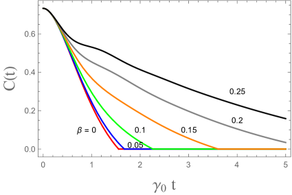
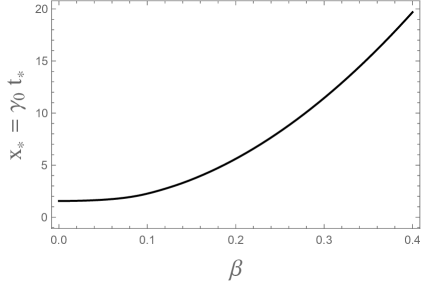
Figure 4: (Color online) (a) Plot of ${\cal C}(t)$ with choosing $\beta=0,0.05,0.1,0.15,0.2,0.25$ when other parameters are fixed as $a=0.4$, $\lambda=2\gamma_{0}$, $\omega_{0}=20\gamma_{0}$, and $\Delta=0$. The time domain $0\leq x\leq x_{*}\equiv\gamma_{0}t_{*}$ for nonvanishing entanglement becomes larger and larger with increasing $\beta$. (b) Plot of $\beta$-dependence of $x_{*}$ when same values of other parameters are chosen. As expected, $x_{*}$ increases with increasing $\beta$ quadratically. (see Eq. (31)

The effect of the particle velocity $\beta$ on the ESD phenomenon is examined in Fig. 4. It is worthwhile noting that the $\beta$-dependence in cubic equation (21) is only through $u_{\pm}$ given in Eq. (22). Since we will choose $x_{1}=2$ and $x_{3}=0$ in Fig. 3 for introducing Markovian environment and removing the effect of $\Delta$, we choose $x_{2}=20$ for considerable change of $u_{\pm}$. In Fig. 4(a) we plot $\gamma_{0}t$-dependence of ${\cal C}(t)$ with varying $\beta$ when other parameters are fixed as $a=0.4$, $\lambda=2\gamma_{0}$, $\omega_{0}=20\gamma_{0}$, and $\Delta=0$. As this figure exhibits, ESD phenomenon occurs regardless of $\beta$ even though the time domain $0\leq x\leq x_{*}\equiv\gamma_{0}t_{*}$, where the bipartite entanglement is alive, becomes larger with increasing $\beta$. This is why the entanglement can be protected in the Markovian environment by making use of $\beta$. In Fig. 4(b) the $\beta$-dependence of $x_{*}$ is plotted. This curve can be fitted as

$$\gamma_{0}t_{*}\approx 126.638\beta^{2}-5.21879\beta+1.57892.$$ (31)

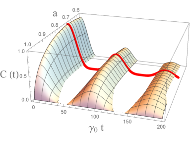
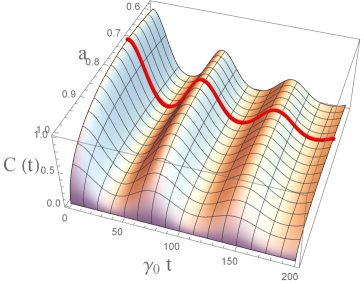
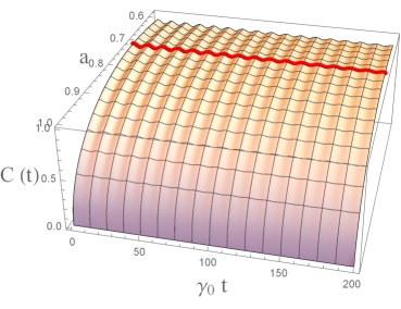
Figure 5: (Color online) We plot $(a,\gamma_{0}t)$-dependence of ${\cal C}(t)$ when $\lambda=0.005\gamma_{0}$, $\beta=0$, and (a) $\Delta=0$, (b) $\Delta=0.05\gamma_{0}$, (c) $\Delta=0.5\gamma_{0}$. Fig. 5(a) exhibits a ROE phenomenon evidently. However, this phenomenon disappears in Fig. 5(b). This means that the small increase of $\Delta$ lifts a minimum of ${\cal C}(t)$ slightly from zero. Fig. 5(c) exhibits a rapid oscillatory behavior of $C(t)$ whose amplitude is very small. As a result, the entanglement does not decrease with the lapse of time. In this way the entanglement can be protected in the non-Markovian environment by making use of the detuning parameter $\Delta$.

Now, we examine the effect of $\beta$ and $\Delta$ on the ROE phenomenon in non-Markovian environment. First, we consider the effect of $\Delta$ in Fig. 5. In Fig. 5(a) we plot $(a,\gamma_{0}t)$-dependence of ${\cal C}(t)$ when $\lambda=0.005\gamma_{0}$ and $\beta=\Delta=0$. The line is correspondent to maximal entanglement initial state, that is, $a=1/\sqrt{2}$. The disconnection of wiggles in Fig. 5(a) shows the ER phenomenon evidently. In Fig. 5(b) we increase $\Delta$ slightly as $\Delta=0.05\gamma_{0}$ without change of other parameters. Although there are wiggles like Fig. 5(a), the wiggles in Fig. 5(b) are connected to each other. This means that the ROE phenomenon does not occur. In Fig. 5(c) we increase $\Delta$ again as $\Delta=0.5\gamma_{0}$. This figure shows many wiggles, whose amplitude is very small. As a result, the entanglement does not decrease with the lapse of time. In this way the entanglement can be protected in the presence of non-Markovian environment by making use of the detuning parameter $\Delta$.

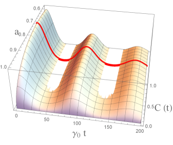
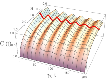
Figure 6: (Color online) We plot $(a,\gamma_{0}t)$-dependence of ${\cal C}(t)$ when $\lambda=0.005\gamma_{0}$, $\omega_{0}=20\gamma_{0}$, $\Delta=0$, and (a) $\beta=0.003$, (b) $\beta=0.01$. When $\beta=0$, Fig. 5(a) is reproduced. As Fig. 6(a) exhibits, the ROE phenomenon occurs at most range of $a$ because $\beta$ is very small. Even in this case, however, the ROE phenomenon disappears at the large $a$ region. In Fig. 6(b) the ROE phenomenon does not occur in the full range of $a$. Similar to Fig. 5(c) the amplitude of an oscillatory behavior of ${\cal C}(t)$ becomes small. This makes a protection of entanglement even in the presence of the non-Markovian environment.

The effect of the particle velocity in the ROE phenomenon is examined in Fig. 6. When $\lambda=0.005\gamma_{0}$, $\beta=\Delta=0$, and $\omega_{0}=20\gamma_{0}$, the $(a,\gamma_{0}t)$-dependence of ${\cal C}(t)$ is exactly the same with Fig. 5(a). This is because of the fact that the cubic equation (21) is independent of $x_{2}$ when $\beta=0$. If we change $\beta$ slightly as $\beta=0.003$, the $(a,\gamma_{0}t)$-dependence of ${\cal C}(t)$ is changed into Fig. 6(a). As this figure shows, the ROE phenomenon does occur at most range of $a$. Even in this case, however, the ROE phenomenon disappears at the large $a$ region due to the small increment of $\beta$. If we increase $\beta$ to $0.01$, the $(a,\gamma_{0}t)$-dependence of ${\cal C}(t)$ becomes Fig. 6(b). The ROE phenomenon does not occur in the full range of $a$. Similar to Fig. 5(c) the amplitude of an oscillatory behavior of ${\cal C}(t)$ becomes small. This makes the reduction of decoherence effect in the non-Markovian environment.

In this paper we explore analytically the effect of particle velocity $\beta=v/c$ and detuning parameter $\Delta$ in the entanglement dynamics when Markovian or non-Markovian environment is present. In particular, we examine the ESD and ROE phenomena in the Markovian and non-Markovian regimes, respectively. As Fig. 3 and Fig. 4 show, the ESD phenomenon always occurs even when $\beta$ or $\Delta$ is nonzero. The difference from a case of $\beta=0$ or $\Delta=0$ is that the time region $0\leq\gamma_{0}t\leq\gamma_{0}t_{*}$ for nonvanishing entanglement becomes wider when $\beta$ or $\Delta$ becomes larger. The $\Delta$- and $\beta$-dependence of $\gamma_{0}t_{*}$ are plotted in Fig. 3(b) and Fig. 4(b). Roughly speaking, this region increases quadratically as a function of $\Delta/\gamma_{0}$ or $\beta$.

The ROE phenomenon in the non-Markovian environment is examined in Fig. 5 and Fig. 6. As these figures show, the ROE phenomenon appearing in $\beta=0$ or $\Delta=0$ (see Fig. 5(a)) disappears for nonzero $\beta$ or nonzero $\Delta$. If $\beta$ or $\Delta$ increases more and more, the amplitude of oscillatory behavior of ${\cal C}(t)$ becomes smaller and smaller in the time domain. In this way, the initial entanglement is not reduced rapidly even in the presence of the non-Markovian environment.

In this paper we consider only the continuum limit ($\tau=\ell/c\rightarrow\infty$). In the real physical setting, however, this limit is only approximation. Presumably, the effect of $\beta$ or $\Delta$ is more drastic for finite $\tau$. In this case, however, the analytic calculation seems to be impossible because the convolution theorem used in this paper cannot be applied.

References

- (1) R. Horodecki, P. Horodecki, M. Horodecki, and K. Horodecki, Quantum Entanglement, Rev. Mod. Phys. 81 (2009) 865 [quant-ph/0702225] and references therein.
- (2) C. H. Bennett, G. Brassard, C. Cr´epeau, R. Jozsa, A. Peres and W. K. Wootters, Teleporting an Unknown Quantum State via Dual Classical and Einstein-Podolsky-Rosen Channles, Phys.Rev. Lett. 70 (1993) 1895.
- (3) C. H. Bennett and S. J. Wiesner, Communication via one- and two-particle operators on Einstein-Podolsky-Rosen states, Phys. Rev. Lett. 69 (1992) 2881.
- (4) V. Scarani, S. Lblisdir, N. Gisin and A. Acin, Quantum cloning, Rev. Mod. Phys. 77 (2005) 1225 [quant-ph/0511088] and references therein.
- (5) A. K. Ekert, Quantum Cryptography Based on Bell’s Theorem, Phys. Rev. Lett. 67 (1991) 661.
- (6) M. A. Nielsen and I. L. Chuang, Quantum Computation and Quantum Information (Cambridge University Press, Cambridge, England, 2000).
- (7) G. Vidal, Efficient classical simulation of slightly entangled quantum computations, Phys. Rev. Lett. 91 (2003) 147902 [quant-ph/0301063].
- (8) T. Yu and J. H. Eberly, Phonon decoherence of quantum entanglement: Robust and fragile states, Phys. Rev. B 66 (2002) 193306 [quant-ph/0209037].
- (9) C. Simon and J. Kempe, Robustness of multiparty entanglement, Phys. Rev. A 65 (2002) 052327 [quant-ph/0109102].
- (10) W. Dür and H. J. Briegel, Stability of Macroscopic Entanglement under Decoherence, Phys. Rev. Lett. 92 (2004) 180403 [quant-ph/0307180].
- (11) T. Yu and J. H. Eberly, Finite-Time Disentanglement Via Spontaneous Emission, Phys. Rev. Lett. 93 (2004) 140404 [quant-ph/0404161].
- (12) T. Yu and J. H. Eberly, Sudden Death of Entanglement: Classical Noise Effects, Opt. Commun. 264 (2006) 393 [quant-ph/0602196].
- (13) T. Yu and J. H. Eberly, Quantum Open System Theory: Bipartite Aspects. Phys. Rev. Lett. 97 (2006) 140403 [quant-ph/0603256]
- (14) T. Yu and J. H. Eberly, Sudden Death of Entanglement, Science, 323 (2009) 598 [arXiv:0910.1396 (quant-ph)].
- (15) M.P. Almeida et al, Environment-induced Sudden Death of Entanglement, Science 316 (2007) 579 [quant-ph/0701184].
- (16) J. Laurat, K. S. Choi, H. Deng, C. W. Chou, and H. J. Kimble, Heralded Entanglement between Atomic Ensembles: Preparation, Decoherence, and Scaling, Physics. Rev. Lett. 99 (2007) 180504 [arXiv:0706.0528 (quant-ph)].
- (17) H. -P. Breuer and F. Petruccione, The Theory of Open Quantum Systems (Oxford University Press, Oxford, New York, 2002).
- (18) B. Bellomo, R. Lo Franco, and G. Compagno, Non-Markovian Effects on the Dynamics of Entanglement, Phys. Rev. Lett. 99 (2007) 160502 [arXiv:0804.2377 (quant-ph)].
- (19) S. Hill and W. K. Wootters, Entanglement of a pair of quantum bits, Phys. Rev. Lett. 78 (1997) 5022 [quant-ph/9703041; W. K. Wootters, Entanglement of Formation of an Arbitrary State of Two Qubits, Phys. Rev. Lett. 80 (1998) 2245 [quant-ph/9709029].
- (20) H. -P. Breuer, E. -M. Laine, and J. Piilo, Measure for the Degree of Non-Markovian Behavior of Quantum Processes in Open Systems, Phys. Rev. Lett. 103 (2009) 210401 [arXiv:0908.0238 (quant-ph)].
- (21) B. Vacchini, A. Smirne, E. -M. Laine, J. Piilo, and H. -P. Breuer, Markovian and non-Markovian dynamics in quantum and classical systems, New J. Phys. 13 (2011) 093004 [arXiv:1106.0138 (quant-ph)].
- (22) D. Chruściński, A. Kossakowski, and A. Rivas, Measures of non-Markovianity: Divisibility versus backflow of information, Phys. Rev. A 83 (2011) 052128 [arXiv:1102.4318 (quant-ph)].
- (23) A. Rivas, S. F. Huelga, and M. B. Plenio, Quantum Non-Markovianity: characterization, quantification and detection, Rep. Prog. Phys. 77 (2014) 094001 [arXiv:1405.0303 (quant-ph)].
- (24) M. J. W. Hall, J. D. Cresser, L. Li, and E. Andersson Canonical form of master equations and characterization of non-Markovianity, Phys. Rev. A 89 (2014) 042120 [arXiv:1009.0845 (quant-ph)].
- (25) K .-I. Kim, H .-M. Li, and B. -K. Zhao, GenuineTripartite Entanglement Dynamics and Transfer in a Triple Jaynes-Cummings Model, Int. J. Theor. Phys. 55 (2016) 241.
- (26) D. K. Park, Tripartite entanglement dynamics in the presence of Markovian or non-Markovian environment, Quantum Inf. Process. 15 (2016) 3189 [arXiv:1601.00273 (quant-ph)].
- (27) S. Das and G. S. Agarwal, Protecting bipartite entanglement by quantum interferences, Phys. Rev. A 81 (2010) 052341 [arXiv:1004.0564 (quant-ph)]; Y. Yang, J. Xu, H. Chen, and S. Y. Zhu, Long-lived entanglement between two distant atoms via left-handed materials, Phys. Rev. A 82 (2010) 030304(R); M. Mukhtar, W. T. Soh, T. B. Saw, and J. Gong, Protecting unknown two-qubit entangled states by nesting Uhrig’s dynamical decoupling sequences, Phys. Rev. A 82 (2010) 052338 [arXiv:1009.0399 (quant-ph)]; S. C. Wang, Z. W. Yu, W. J. Zou, and X. B. Wang, Protecting quantum states from decoherence of finite temperature using weak measurement, Phys. Rev. A 89 (2014) 022318 [arXiv:1308.1665 (quant-ph)].
- (28) B. Bellomo, R. L. Franco, S. Maniscalco, and G. Compagno, Entanglement trapping in structured environments, Phys. Rev. 78 (2008) 060302(R) [arXiv:0805.3056 (quant-ph)]; S. Maniscalco, F. Francica, R. L. Zaffino, N. L. Gullo, and F. Plastina, Protecting Entanglement via the Quantum Zeno Effect, Phys. Rev. Lett. 100 (2008) 090503 [arXiv:0710.3914 (quant-ph)]; J. Z. Hu, X. B. Wang, and L. C. Kwek, Protecting two-qubit quantum states by -phase pulses, Phys. Rev. A 82 (2010) 062317 [arXiv:1011.3460 (quant-ph)]; C. Addis, F. Ciccarello, M. Cascio, G. M. Palma and S. Maniscalco, Dynamical decoupling efficiency versus quantum non-Markovianity, New J. Phys. 17 (2015) 123004 [arXiv:1502.02528 (quant-ph)]; R. L. Franco, Switching quantum memory on and off, New J. Phys. 17 (2015) 081004; Z. X. Man, Y. J. Xia, and R. L. Franco, Harnessing non-Markovian quantum memory by environmental coupling, Phys. Rev. A 92 (2015) 012315 [arXiv:1506.08293 (quant-ph)]; Z. X. Man, N. B. An, and Y. J. Xia, Non-Markovianity of a two-level system transversally coupled to multiple bosonic reservoirs, Phys. Rev. A 90, (2014) 062104; R. L. Franco, B. Bellomo, E. Andersson, and G. Compagno, Revival of quantum correlations without system-environment back-action, Phys. Rev. A 85 (2012) 032318; B. Leggio, R. L. Franco, D. O. Soares-Pinto, P. Horodecki, and G. Compagno, Distributed correlations and information flows within a hybrid multipartite quantum-classical system, Phys. Rev. A 92 (2015) 032311 [arXiv:1508.04736 (quant-ph)]; A. D’Arrigo, G. Benenti, R. L. Franco, G. Falci, and E. Paladino, Hidden entanglement, system-environment information flow and non-Markovianity, Int. J. Quantum Inf. 12 (2014) 1461005 [arXiv:1402.1948 (quant-ph)]; A. Z. Chaudhry and J. Gong, Decoherence control: Universal protection of two-qubit states and two-qubit gates using continuous driving fields, Phys. Rev. A 85 (2012) 012315 [arXiv:1110.4695 (quant-ph)].
- (29) A. Mortezapour, M. A. Borji, and R. L. Franco, Protecting entanglement by adjusting the velocities of moving qubits inside non-Markovian environments, arXiv:1702.07996 (quant-ph).
- (30) K. Kraus, States, Effect, and Operations: Fundamental Notions in Quantum Theory (Springer-Verlag, Berlin, 1983).