On microscopic structure of the QCD vacuum

Abstract

We propose a new class of regular stationary axially symmetric solutions in a pure QCD which correspond to monopole-antimonopole pairs at macroscopic scale. The solutions represent vacuum field configurations which are locally stable against quantum gluon fluctuations in any small space-time vicinity. This implies that the monopole-antimonopole pair can serve as a structural element in microscopic description of QCD vacuum formation through the monopole pair condensation.

I Introduction

One of most attractive mechanisms of confinement is based on idea that the vacuum in quantum chromodynamics (QCD) vacuum represents a dual superconductor which is formed due to condensation of color magnetic monopoles nambu74 ; mandelstam76 ; polyakov77 ; thooft81 . Realization of this idea in the framework of a rigorous theory has not been possible due to two principal difficulties: the first one, the color monopoles as physical particles have not been found in experiment, and so far there is no strict theoretical evidence of their existence in the real QCD (except unphysical singular monopole solutions). The second obstacle represents a long-standing problem of vacuum stability since late 70s when it was shown that Savvidy-Nielsen-Olesen vacuum is unstable savv ; N-O . There have been numerous attempts to resolve this issue. Unfortunately, most of vacuum models lack the local vacuum stability at microscopic space-time scale. Besides, the known approaches to vacuum problem are based on assumption that vacuum field is static. Such an assumption is not consistent with the quantum mechanical principle which implies that elementary vacuum fields (vortices, monopoles etc.) should vibrate at the microscopic level niel-oles1 ; amb-oles1 .

In the present Letter we explore a novel approach for a microscopic description of the QCD vacuum based on stationary vacuum field configurations. There are several no-go theorems which impose strict limitations on the existence of finite energy static and stationary solutions in a pure Yang-Mills theory derr64 ; deser76 ; pagels77 ; coleman77 . To overcome the restrictions imposed by these no-go theorems, it was proposed in past that classical stationary non-solitonic inifnite energy wave solutions with a finite energy density may correspond to quasi-particles or to vacuum states in the quantum theory jackiw77 . Recently an example of a regular stationary spherically symmetric solution with a finite energy density in a pure QCD has been proposed ijmpa2017 . The solution represents a system of interacting static Wu-Yang monopole and time dependent off-dagonal gluon field. It has been proved that such a solution is stable against quantum gluon fluctuations prd2017 . We generalize these results to the case of axially-symmetric fields and construct a new class of regular axially symmetric periodic wave type solutions with a finite energy density in a pure $SU(2)$ and $SU(3)$ QCD. The solutions possess an intrinsic mass parameter which determines a microscopic space-time scale. The averaging over the time period implies that the proposed solutions can be treated as non-topological non-Abelian monopole-antimonopole pairs. The most important result is that our solutions are locally stable under quantum gluon fluctuations in any small vicinity of each space point. The solutions can be served as structural elements of the QCD vacuum formed through the monopole pair condensation in analogy with the Cooper electron pair condensation in the ordinary superconductor.

II Axially-symmetric stationary solutions in $SU(2)$ QCD

We start with a standard Lagrangian of a pure $SU(N)$ Yang-Mills theory and corresponding equations of motion

$${\cal L}_{0}=-\dfrac{1}{4}F_{\mu\nu}^{a}F^{a\mu\nu},$$

$$(D^{\mu}F_{\mu\nu})^{a}=0,$$ (1)

where $(a=1,2,..,N)$ denote the color indices, and $(\mu,\nu=r,\theta,\varphi,t)$ are the space-time indices in the spherical coordinates. Let us first consider stationary solutions in a pure $SU(2)$ QCD. One can generalize a static axially symmetric Dashen-Hasslacher-Neveu (DHN) ansatz DHN as follows

$$A_{r}^{2} = K_{1}(r,\theta,t),~{}~{}A_{\theta}^{2}=K_{2}(r,\theta,t),~{}~{}A_{\varphi}^{3}=K_{3}(r,\theta,t),$$

$$A_{\varphi}^{1} = K_{4}(r,\theta,t),~{}~{}~{}A_{t}^{2}=K_{5}(r,\theta,t).$$ (2)

The ansatz leads to a system of five differential equations which are invariant under residual $U(1)$ gauge transformations with a gauge parameter $\lambda(r,\theta,t)$ Manton78 ; RR ; KKB

$$K^{\prime}_{1} = K_{1}\partial_{r}\lambda,~{}~{}K^{\prime}_{2}=K_{2}+\partial_{\theta}\lambda,~{}~{}K^{\prime}_{5}=K_{5}+\partial_{t}\lambda,$$

$$K_{3}^{\prime} = K_{3}\cos\lambda+K_{4}\sin\lambda,$$

$$K_{4}^{\prime} = K_{4}\cos\lambda-K_{3}\sin\lambda.$$ (3)

To fix the residual symmetry we choose a Lorenz gauge by introducing the gauge fixing terms

$${\cal L}_{g.f.}^{\small{SU(2)}} = -\dfrac{1}{2}(\partial_{r}K_{1}+\dfrac{1}{r^{2}}\partial_{\theta}K_{2}-\partial_{t}K_{5})^{2}.$$ (4)

We apply a method used in solving equations for the sphaleron solution RR ; KKB . First, we decompose the functions $K_{i}$ in the Fourier series

$$K_{i=1-4}(r,\theta,t) = \delta_{i4}C_{4}+$$

$$\sum_{n=1,2,...}\tilde{K}_{i}^{(n)}(nMr,\theta)\cos(nMt),$$

$$K_{5}(r,\theta,t) = \sum_{n=1,2,...}\tilde{K}_{5}^{(n)}(nMr,\theta)\sin(nMt),$$ (5)

where $C_{4}$ is an arbitrary number, $M$ is a mass scale parameter which defines a class of conformally equivalent field configurations due to the presence of scaling invariance in a pure QCD, $(r\rightarrow Mr,t\rightarrow Mt)$. The structure of the series expansion (5) implies that all time averaged color electric components of the field strength $F_{\mu\nu}^{a}$ vanish identically. Substituting the series decomposition truncated at a finite order $n_{f}$ into the classical action, and performing integration over the time period, one results in a reduced action which implies Euler equations for the coefficient functions $\tilde{K}_{i}^{(n\leq n_{f})}(r,\theta)$. The obtained reduced equations for the modes $\tilde{K}_{i}^{(n\leq n_{f})}(r,\theta)$ represent a well-defined system of elliptic partial differential equations which can be solved by applying standard numeric recipes.

To solve the equations for $\tilde{K}_{i}^{(n\leq n_{f})}(r,\theta)$ we impose the following Dirichlet boundary conditions

$${\tilde{K}}_{i}^{(n)}(r,\theta)|_{r=0}=0,~{}~{}~{}{\tilde{K}}_{i}^{(n)}(r,\theta)|_{\theta=0,\pi}=0.$$ (6)

Asymptotic behavior at ($r\rightarrow\infty$) of the functions ${\tilde{K}}_{i}^{(n)}$ is determined by the equations of motion as follows

$${\tilde{K}}_{1}^{(n)}\simeq a_{1}^{(n)}(\theta)\dfrac{\sin(nMr)}{r^{2}},~{}~{}~{}{\tilde{K}}_{5}^{(n)}\simeq a_{5}^{(n)}(\theta)\dfrac{\cos(nMr)}{r^{2}},$$

$${\tilde{K}}_{2,3,4}^{(n)}\simeq a_{2,3,4}^{(n)}(\theta)\cos(nMr),$$ (7)

where $a_{i}^{(n)}(\theta)$ are periodic angle functions. We choose the lowest angle modes for $a_{i}^{(n)}(\theta)$ consistent with the finite energy density condition, in particular, in the leading order one has $a_{i\neq 2}^{(1)}(\theta)=c_{i}\sin^{2}\theta$, $a_{2}^{(1)}(\theta)=c_{2}\sin(2\theta)$. With this one can solve numerically the equations up to the sixth order of series decomposition in the numeric domain $(0\leq r\leq L,0\leq\theta\leq\pi)$. The obtained numeric solution implies that even order coefficient functions $\tilde{K}_{1,2,3,5}^{(n=2k)}$ and odd order functions $\tilde{K}_{4}^{(n=2k-1)}$ vanish identically. A typical solution in the leading and subleading order approximation is presented in Fig. 1.

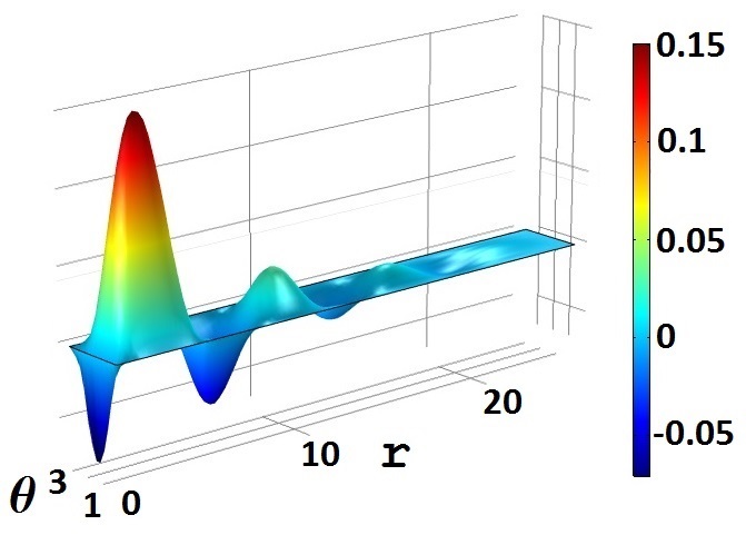
(a)  

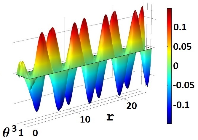
(b)  

(c)  

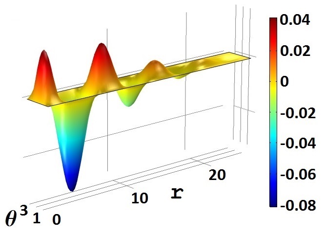
(d)  

(e)  

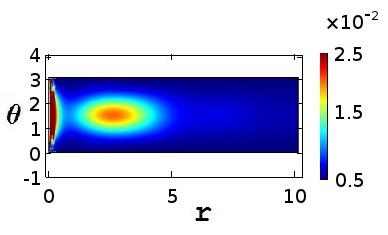
(f)  

Figure 1: Solution profile functions in the leading and sub-leading order: (a) ${\tilde{K}}_{1}^{(1)}$; (b) ${\tilde{K}}_{2}^{(1)}$; (c) ${\tilde{K}}_{3}^{(1)}$; (d) ${\tilde{K}}_{5}^{(1)}$; (e) ${\tilde{K}}_{4}^{(2)}$; (f) the energy density plot ($C_{4}=2,g=1,M=1$).

One has fast convergence for the obtained numeric solution. The solution profile functions of the third and fourth order, $\tilde{K}_{i}^{(n=3,4)}$, provide corrections less than $2\%$ by a norm with respect to the solution obtained in the leading and subleading order. The fifth and sixth order corrections are less than $0.1\%$. The energy density has an absolute maximum at the origin and a local maximum along the torus center line in the plane $\theta=\pi/2$. For large values of the radius of the sphere enclosing the numeric domain, the energy density decreases as $\dfrac{1}{R^{2}}$.

In the leading order one has non-vanishing time averaged color magnetic fields $\langle F_{\theta\varphi}^{1}\rangle_{t}\simeq{\tilde{K}}_{2}^{(1)}{\tilde{K}}_{3}^{(1)}$ and $\langle F_{r\varphi}^{1}\rangle_{t}\simeq{\tilde{K}}_{1}^{(1)}{\tilde{K}}_{3}^{(1)}$, which create magnetic fluxes corresponding to a pair of non-topological monopole and antimonopole located at the origin. It is unexpected that a regular monopole-antimonopole pair solution in the limit of zero distance between the monopoles does exist in the real QCD. A brief overview of the structure of non-Abelian monopole-antimonopole fields and details of the numeric solution are presented in SM .

III Axially-symmetric stationary solutions in $SU(3)$ QCD

We are looking for essentially $SU(3)$ field configurations which do not reduce to embedded $SU(2)$ solutions. We start with a more general Lagrangian which includes additional gauge fixing terms

$${\cal L}_{gen} = {\cal L}_{0}-\sum_{a=2,5,7}\dfrac{\alpha_{a}}{2}(\partial_{r}A^{a}_{1}+\dfrac{1}{r^{2}}\partial_{\theta}A^{a}_{2}-\partial_{t}A_{4}^{a})^{2},$$

where $\alpha_{a}$ are arbitrary real numbers. An axially symmetric ansatz contains the following non-vanishing components of the gauge potential corresponding to three $I,U,V$-type $SU(2)$ subgroups of $SU(3)$

$$A_{1}^{2} = K_{1},~{}~{}A_{2}^{2}=K_{2},~{}~{}A_{3}^{1}=K_{4},~{}~{}A_{4}^{2}=K_{5},$$

$$A_{1}^{5} = Q_{1},~{}~{}A_{2}^{5}=Q_{2},~{}~{}A_{3}^{4}=Q_{4},~{}~{}A_{4}^{5}=Q_{5},$$

$$A_{1}^{7} = S_{1},~{}~{}~{}A_{2}^{7}=S_{2},~{}~{}A_{3}^{6}=S_{4},~{}~{}~{}A_{4}^{7}=S_{5},$$

$$A_{3}^{3} = K_{3},~{}~{}~{}A_{3}^{8}=K_{8},$$ (9)

where the fields $K_{i},Q_{i},S_{i}$ depend on space-time coordinates $(r,\theta,t)$. The ansatz is consistent with the Euler equations obtained from the Lagrangian ${\cal L}_{gen}$ and leads to a system of fourteen partial differential equations for the field variables $K_{i},Q_{i},S_{i}$. Note, that due to the introduced gauge fixing terms the equations for $K_{i},Q_{i},S_{i}$ do not admit any residual symmetry and represent well-defined second order hyperbolic differential equations.

One can simplify further the system of equations for $K_{i},Q_{i},S_{i}$ applying the following reduction ansatz

$$Q_{1,2,5}=-S_{1,2,5}=-K_{1,2,5},$$

$$Q_{4}=\big{(}-\frac{1}{2}+\frac{\sqrt{3}}{2}\big{)}K_{4},$$

$$S_{4}=\big{(}-\frac{1}{2}-\frac{\sqrt{3}}{2}\big{)}K_{4},$$

$$K_{3,8}=-\frac{\sqrt{3}}{2}K_{4},$$ (10)

with setting the parameters $\alpha_{2}=\alpha_{5}=\alpha_{7}$. Without loss of generality we choose $\alpha_{a}=1$. Direct substitution of the reduction ansatz into the equations for $K_{i},Q_{i},S_{i}$ leads to only five linearly independent differential equations which contain four second order hyperbolic equations for the fields $K_{1,2,4,5}(r,\theta,t)$ and one quadratic constraint with first order partial derivatives

$$r^{2}\partial_{t}^{2}K_{1}-r^{2}\partial_{r}^{2}K_{1}-\partial_{\theta}^{2}K_{1}+2r(\partial_{t}K_{5}-\partial_{r}K_{1})$$

$$+\cot\theta(\partial_{r}K_{2}-\partial_{\theta}K_{1})+\dfrac{9}{2}\csc^{2}\theta K_{4}^{2}K_{1}=0,$$ (11)

$$r^{2}\partial_{t}^{2}K_{2}-r^{2}\partial_{r}^{2}K_{2}-\partial_{\theta}^{2}K_{2}+r^{2}\cot\theta(\partial_{t}K_{5}-\partial_{r}K_{1})$$

$$-\cot\theta\partial_{\theta}K_{2}+\dfrac{9}{2}\csc^{2}\theta K_{4}^{2}K_{2}=0,$$ (12)

$$r^{2}\partial_{t}^{2}K_{4}-r^{2}\partial_{r}^{2}K_{4}-\partial_{\theta}^{2}K_{4}+\cot\theta\partial_{\theta}K_{4}$$

$$+3r^{2}(K_{1}^{2}-K_{5}^{2})K_{4}+3K_{2}^{2}K_{4}=0,$$ (13)

$$r^{2}\partial_{t}^{2}K_{5}-r^{2}\partial_{r}^{2}K_{5}-\partial_{\theta}^{2}K_{5}+2r(\partial_{t}K_{1}-\partial_{r}K_{5})$$

$$+\cot\theta(\partial_{t}K_{2}-\partial_{\theta}K_{5})+\dfrac{9}{2}\csc^{2}\theta K_{4}^{2}K_{5}=0,$$ (14)

$$2r^{2}(K_{5}\partial_{t}K_{4}-K_{1}\partial_{r}K_{4})+K_{2}(\cot\theta K_{4}-2\partial_{\theta}K_{4})$$

$$+K_{4}(-\partial_{\theta}K_{2}+r^{2}(\partial_{t}K_{5}-\partial_{r}K_{1}))=0.$$ (15)

The system of equations (11-15) is not suitable for numeric solving due to the presence of the constraint with derivatives and lack of explicit functions defining the boundary conditions on two-dimensional surfaces closing the three-dimensional numeric domain. To overcome this problem we employ the same method as in the case of $SU(2)$ QCD using the Fourier series decomposition for the fields $K_{i},Q_{i},S_{i}$ as in (5) (the Abelian potential $K_{8}$ has a decomposition similar to one for $K_{3}$). After integration over the time period in the classical action one can derive the Euler equations for the field modes ${\tilde{K}}_{i}^{(n)},{\tilde{Q}}_{i}^{(n)},{\tilde{S}}_{i}^{(n)}$ depending on two coordinates $(r,\theta)$. We apply a reduction ansatz to the obtained Euler equations for ${\tilde{K}}_{i}^{(n)},{\tilde{Q}}_{i}^{(n)},{\tilde{S}}_{i}^{(n)}$

$${\tilde{Q}}_{1,2,5}^{(n)}=-{\tilde{S}}_{1,2,5}^{(n)}=-{\tilde{K}}_{1,2,5}^{(n)},$$

$${\tilde{Q}}_{4}^{(n)}=\big{(}-\frac{1}{2}+\frac{\sqrt{3}}{2}\big{)}{\tilde{K}}_{4}^{(n)},$$

$${\tilde{S}}_{4}^{(n)}=\big{(}-\frac{1}{2}-\frac{\sqrt{3}}{2}\big{)}{\tilde{K}}_{4}^{(n)},$$

$${\tilde{K}}_{3,8}^{(n)}=-\frac{\sqrt{3}}{2}{\tilde{K}}_{4}^{(n)},$$ (16)

where ($n=1,3,5,...$), and we impose a condition that all even modes ${\tilde{K}}_{i}^{(2k)},{\tilde{Q}}_{i}^{(2k)},{\tilde{S}}_{i}^{(2k)}$ vanish. Such a condition resolves the constraint (15) and reduces the space of general solutions to the subspace of solutions with a definite parity under the reflection $\theta\rightarrow\pi-\theta$. It is remarkable that the ansatz (16) reduces the total number of equations to four independent second order hyperbolic equations in each order of the Fourier series decomposition (5) without any additional constraints.

Note that the Abelian potentials ${\tilde{K}}_{3,8}$ are equal to each other as it takes place in the case of Abelian Weyl symmetric homogeneous magnetic fields providing an absolute minimum of the quantum effective potential flyvb ; pakMPLA06 .

We demonstrate existence of another type of monopole pair solution which is different from the $SU(2)$ stationary monopole pair considered above. To find such a solution we apply asymptotic conditions (7) for the functions $\tilde{K}_{i}^{(n)}$ containing even angle modes $a_{2,4}^{(n)}(\theta)$ and odd angle modes $a_{1,5}^{(n)}(\theta)$. Imposing vanishing Dirichlet boundary conditions at the origin and along the boundaries $(\theta=0,\pi)$, we solve the equations for ${\tilde{K}}_{i}^{(n)}$ in the fifth order approximation. The obtained solution profile functions ${\tilde{K}}_{i}^{(1)}$ and energy density plots are presented in Fig. 2.

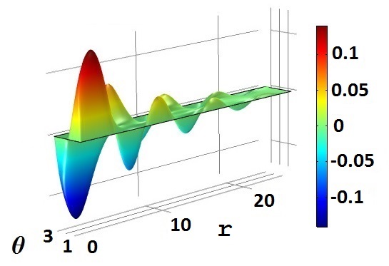
(a)  

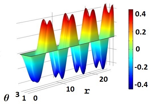
(b)  

(c)  

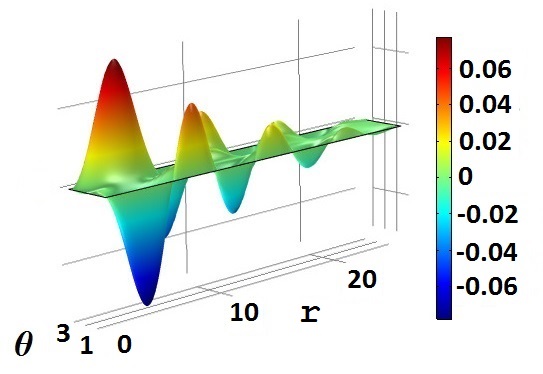
(d)  

(e)  

(f)  

Figure 2: Profile functions for the monopole pair solution in the leading order: (a) ${\tilde{K}}_{1}^{(1)}$; (b) ${\tilde{K}}_{2}^{(1)}$; (c) ${\tilde{K}}_{4}^{(1)}$; (d) ${\tilde{K}}_{5}^{(1)}$; (e) the energy density plot; (f) the energy density contour plot in Cartesian coordinates ($g=1,M=1$).

Consider the magnetic flux structure of the obtained solution when the observation time is much larger than the period of time oscillations. The time averaged radial components of the Abelian field strength in the leading order include only non-linear terms

$$\langle F_{\theta\varphi}^{3}\rangle_{t}=-\dfrac{3}{4}{\tilde{K}}_{2}^{(1)}{\tilde{K}}_{4}^{(1)}, \langle F_{\theta\varphi}^{8}\rangle_{t}=+\dfrac{3}{4}{\tilde{K}}_{2}^{(1)}{\tilde{K}}_{4}^{(1)},$$ (17)

where the Abelian potential ${\tilde{K}}_{4}^{(1)}$ contains the angle dependent factor $\sin^{2}\theta$, and ${\tilde{K}}_{2}^{(1)}$ is an even function with respect to the reflection symmetry $\theta\rightarrow\pi-\theta$. The magnetic fields ${\tilde{F}}_{\theta\varphi}^{3,8(1)}$ create opposite magnetic fluxes through a sphere of radius $R$ with a center at the origin which correspond to non-topological antimonopole and monopole located at one point. Careful numeric analysis shows that stationary solutions corresponding to a lowest energy in a chosen finite numeric domain are classified by only two parameters, the conformal parameter $M$ and an amplitude $c_{0}$ of the oscillating Abelian potential ${\tilde{K}}_{4}^{(1)}$. A detailed structure of the numeric solution up to the fifth order series decomposition is given in SM .

IV Microscopic quantum stability of the stationary solutions

The Savvidy QCD vacuum based on the classical homogeneous color magnetic field is unstable due to the presence of an imaginary part of the effective action savv ; N-O . Usually one expects that introducing time dependent color fields as vacuum makes worse the vacuum stability since the color electric field leads to an imaginary part of the effective action as well schan82 . Surprisingly, it has been found that non-linear plane wave solutions make the problem of vacuum stability more soft, in a sense, that an equation for the unstable modes is very similar to the equation for an electron in the periodic potential ijmpa2017 . This gives a hint that one can find a proper stationary periodic wave type solution which provides a stable vacuum. Indeed, recently it has been proved that a stationary spherically symmetric generalized Wu-Yang monopole solution leads to a stable vacuum prd2017 . We will prove the quantum stability of the stationary axially-symmetric solutions under small quantum gluon fluctuations in the case of $SU(2)$ and $SU(3)$ QCD.

To verify the stability of the solutions it is suitable to apply the quantum effective action formalism. We consider one-loop quantum effective action expressed in terms of functional operators chopakprd02

$$S^{\rm 1loop}_{\rm eff} = -\dfrac{1}{2}{\rm Tr}\ln[K_{\mu\nu}^{ab}]+{\rm Tr}\ln[M_{\rm FP}^{ab}],$$

$$K_{\mu\nu}^{ab} = -\delta^{ab}\delta_{\mu\nu}\partial^{2}_{t}-\delta_{\mu\nu}({\mathscr{D}}_{\rho}{\mathscr{D}}^{\rho})^{ab}-2f^{acb}{\mathscr{F}}_{\mu\nu}^{c},\quad$$ (18)

$$M_{\rm FP}^{ab} = -({\mathscr{D}}_{\rho}{\mathscr{D}}^{\rho})^{ab},$$

where the Wick rotation $t\rightarrow-it$ has been performed to provide the causal structure of the operators, and ${\mathscr{D}}_{\mu},{\mathscr{F}}_{\mu\nu}^{c}$ are defined with a classical background field $\mathscr{B}_{\mu}^{a}$. The operators $K_{\mu\nu}^{ab}$ and $M^{ab}_{\rm FP}$ correspond to gluon and Faddeev-Popov ghosts. Note that the expression (18) is valid for arbitrary background field and does not depend on a chosen gauge for the background field due to use of a gauge covariant background formalism abbott . Effective action describes the vacuum-vacuum amplitude, and the presence of an imaginary part of the action implies vacuum instability. Therefore, if the operator $K_{\mu\nu}^{ab}$ is not positively defined then an unstable mode will appear as an eigenfunction corresponding to a negative eigenvalue of the following “Schrödinger” equation

$$K_{\mu}^{ab}\Psi_{\nu}^{b}=\lambda\Psi_{\mu}^{a},$$ (19)

where the “wave functions” $\Psi_{\mu}^{a}(t,r,\theta,\varphi)$ describe gluon fluctuations. Note that the ghost operator $M^{ab}_{\rm FP}$ is positively defined and does not produce instability N-O . The potential in the operator $K_{\mu}^{ab}$ does not depend on the asimuthal angle. Due to this one can separate a corresponding angle dependent part from the function $\Psi_{\mu}^{a}$ and solve the eigenvalue equation in a three-dimensional domain $(t,r,\theta)$. Substituting interpolation functions for the stationary magnetic solutions in the leading order, one can solve the eigenvalue equation (19). In the case of $SU(2)$ stationary solution a full eigenvalue spectrum is divided into four sub-spectra corresponding to four decoupled systems of equations: (I) $\Psi_{4}^{2}$, (II) $\Psi_{4}^{1},\Psi_{4}^{3}$, (III) $\Psi_{1}^{2},\Psi_{2}^{2},\Psi_{3}^{1},\Psi_{3}^{3}$, (IV) $\Psi_{1}^{1},\Psi_{1}^{3},\Psi_{2}^{1},\Psi_{2}^{3},\Psi_{3}^{2}$. The lowest eigenvalue is positive, and it is reached by a solution satisfying the system of equations (II), the corresponding eigenfunctions are plotted in Fig. 3 ($g=1,M=1$).

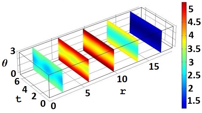
(a)  

(b)  

Figure 3: Non-vanishing eigenfunctions corresponding to the lowest eigenvalue $\lambda=0.05294$: (a) $\Psi_{4}^{1}$; (b) $\Psi_{4}^{3}$.

Other systems of equations, (I,III,IV), have a similar structure of the eigenvalue spectrum.

In the case of $SU(3)$ stationary monopole pair solution the equations in (19) are not factorized, and one has to solve a full set of thirty two differential equations. Numerical results of solving the “Schrödinger” eigenvalue equation with the stationary monopole-antimonopole background field show that the eigenvalue spectrum is positively defined. The obtained dependence of the lowest eigenvalue on the size of the chosen numeric domain for large values of $L$ confirms the positiveness of the eigenvalue spectrum, Fig. 4. This proves the quantum stability of stationary monopole-antimonopole pair solutions in QCD.

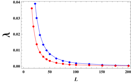
Figure 4: Dependence of the ground state eigenvalue $\lambda(L)$ on the size $L$ of the numeric domain in the cases of $SU(3)$ (red curve) and $SU(2)$ (blue curve) stationary monopole-antimonopole pair solutions ($g=1,M=1$).

The quantum stability of $SU(2)$ and $SU(3)$ stationary background fields has been checked for solutions with amplitude values of the Abelian potential $K_{4}(r,\theta,t)$ in the interval $(0\leq c_{0}\leq 2)$ and with conformal parameter values ($0\leq M\leq 2$). For large values of $M,c_{0}$ unstable modes appears which destabilize the vacuum.

V Weyl symmetry and microscopic structure of the QCD vacuum

Let us consider symmetry properties of essentially $SU(3)$ stationary solutions. The classical Yang-Mills Lagrangian can be rewritten in terms of Weyl symmetric fields pakMPLA06

$${\cal L}_{0} = \sum_{p=1,2,3}\Big{\{}-\dfrac{1}{6}({\cal G}|_{\mu\nu}^{p})^{2}-\dfrac{1}{2}|D_{\mu}^{p}W_{\nu}^{p}-D_{\nu}^{p}W_{\mu}^{p}|^{2}$$ (20)

$$-ig{\cal G}_{\mu\nu}^{p}W_{\mu}^{*p}W_{\nu}^{p}\Big{\}}-{\cal L}_{int}^{(4)}[W],$$

where ${\cal G}_{\mu\nu}^{p}$ are Abelian field strengths containing the gauge potentials $A_{\mu}^{3,8}$, the complex fields $W_{\mu}^{p}$ represent off-diagonal gluons, and the index $p$ counts the Weyl symmetric gauge potentials. Note that the Lagrangian is not Weyl symmetric under permutation of $I,U,V$ subgroups $SU(2)$ since the quartic interaction term ${\cal L}_{int}^{(4)}[W]$ is not factorized into a sum of separate parts corresponding to $I,U,V$ sectors. It is remarkable that the Lagrangian on the space of essentially $SU(3)$ stationary solutions possesses a high symmetric structure. First of all, substituting the reduction ansatz (10) for general functions $K_{i},Q_{i},S_{i}$ into the Lagrangian, one can verify that ${\cal L}_{int}^{(4)}$ obtains an explicit Weyl symmetric form

$${\cal L}_{int}^{(4)}[W]=\dfrac{9}{8}\sum_{p=1,2,3}\Big{(}(W^{*p}_{\mu}W^{p}_{\mu})^{2}-(W^{*}_{\mu})^{2}(W_{\nu})^{2}\Big{)}$$ (21)

Secondly, each $I,U,V$ sector in the Lagrangian (20) contains cubic interaction terms corresponding to the anomaly magnetic moment interaction which is precisely the source of the Nielsen-Olesen vacuum instability N-O . It is surprising, within the framework of the ansatz (10) one has complete mutual cancellation of all cubic interaction terms. This implies that on the space of Weyl symmetric fields the classical action describes a generalized $\lambda\phi^{4}$ theory.

A simple consideration shows that our approach to QCD vacuum problem based on stationary Weyl symmetric monopole pair solutions opens a new perspective towards construction of a microscopic theory of vacuum and vacuum phase transitions. First of all, note that a system of separated stationary generalized Wu-Yang monopoles and antimonopoles can not be stable due mutual attraction between the monopole and antimonopole. In addition, despite on the quantum stability of a sinlge stationary spherically symmetric monopole, the solution is rather classically unstable with respect to small axially-symmetric field deformations ijmpa2017 . This implies that axially-symmetric solutions are more preferable as candidates for the vacuum. Another important feature of the monopole pair solution is that it represents a non-trivial essentially non-Abelian field configuration which describes a pair of monopole and antimonopole located at one point. This implies that monopole and antimonopole, as well as two monopole-antimonopole pairs with opposite color orientations, can merge into a stable state with a finite energy density in the limit of zero distance between the monopole and antimonopole. In other words, the existence of a stable solution for a pair of monopole and antimonopole located at one point prevents from annihilation and disappearance of the monopoles. This is contrary to the case of Dirac and Wu-Yang pair of monopole and antimonopole which annihilate when they meet each other.

We expect that the QCD vacuum is formed due to condensation of monopole-antimonopole pairs, and the microscopic vacuum structure is characterized by few parameters: the conformal parameter $M$, the amplitude of oscillations $c_{0}$ of the Abelian gauge potential $K_{4}$ in the asymptotic region, and the concentration of monopole pairs at zero temperature. Numeric analysis shows that with increasing temperature the internal energy of each monopole pair increases and at some critical values of the parameters ($M>2,c_{0}>2$) the monopole-antimonopole pair becomes unstable. Note that in the confinement phase the vacuum averaging value of the gluon field operator $\langle 0|A_{\mu}^{a}|0\rangle$ vanishes since the size of the hadron is much larger than the characteristic length $\lambda_{M}=2\pi/M$ of the vacuum monopole field oscillations. To describe dynamics of the vacuum structure at finite temperature one should apply the Euclidean functional integral formalism with time integration in the finite interval $(0\leq t\leq\beta=1/kT)$. It is clear that at high enough temperature the upper integration limit $\beta$ will be less than $\lambda_{M}$. This will lead to a non-vanishing vacuum averaging value of the gluon field operator, $\langle 0|A_{\mu}^{a}|0\rangle$, and transition to the deconfinement phase with spontaneous symmetry breaking where the gluon can be observed as a color object.

VI Conclusion

In conclusion, we have proposed a new class of regular axially-symmetric stationary solutions in a pure $SU(2)$ and $SU(3)$ QCD. The solutions possess interesting features such as an intrinsic mass parameter, a vanishing classical canonical spin density. Such properties serve as a heuristic argument to existence of a stable quantum vacuum condensate in the quantum theory. After time averaging over the period the solutions correspond to color magnetic field configurations which have asymptotic behavior similar to one of the non-Abelian monopole-antimonopole pair. A careful numeric analysis confirms stability of the stationary solutions under small gluon fluctuations within the framework of one-loop effective action formalism. As it is known, in QCD the quantum dynamics leads to generation of the mass gap, or the so-called vacuum gluon condensate parameter. So that, the mass scale parameter $M$ of the classical stationary solutions is related to the finite mass gap parameter and characterizes the microscopic scale of the vacuum structure. The presence of such a parameter allows to describe phase transitions in QCD. The most important step in construction of the full microscopic theory of the QCD vacuum is to study condensation of monopole-antimonopole pairs. This will be considered in a separate paper.

- (1) Y. Nambu, Phys. Rev. D10, 4262 (1974).
- (2) S. Mandelstam, Phys. Rep. 23C, 245 (1976).
- (3) A. Polyakov, Nucl. Phys. B120, 429 (1977).
- (4) G. ’t Hooft, Nucl. Phys. B190, 455 (1981).
- (5) G.K. Savvidy, Phys. Lett. B71, 133 (1977).
- (6) N.K. Nielsen and P. Olesen, Nucl. Phys. B144, 376 (1978).
- (7) N.K. Nielsen and P. Olesen, Nucl. Phys. B160, 380 (1979).
- (8) J. Ambjørn and P. Olesen, Nucl. Phys. B170, 60 (1980).
- (9) G.H. Derrick, J. Math. Phys. 5, 1252 (1964).
- (10) S. Deser, Phys. Letters B64, 463 (1976).
- (11) H. Pagels, Phys.Lett. B68, 466 (1977).
- (12) S. Coleman, Comm. Math. Phys., 55, 113 (1977).
- (13) R. Jackiw, Rev. Mod. Phys. 49, 681 (1977).
- (14) B.-H. Lee, Y. Kim, D.G. Pak, T. Tsukioka, P.M. Zhang, Int. J. of Mod. Phys. A, Vol. 32, 1750062 (2017).
- (15) Y. Kim, B.-H. Lee, D.G. Pak, Ch. Park and T. Tsukioka, Phys. Rev. D 96, 054025 (2017).
- (16) R. Dashen, B. Hasslacher and A. Neveu, Phys. Rev. D10 (1974) 4138.
- (17) N.S. Manton, Nucl. Phys. B135, 319 (1978).
- (18) C.Rebbi and P. Rossi, Phys. Rev. D 22, 2010 (1980).
- (19) J. Kunz, B. Kleihaus and Y. Brihaye, Phys. Rev. D 46, 3587 (1992).
- (20) D.G. Pak, B.-H. Lee, Y. Kim, T. Tsukioka and P.M. Zhang, On microscopic structure of the QCD vacuum - Supplemental Material.
- (21) H. Flyvbjerg, Nucl. Phys. B176, 379 (1980).
- (22) Y.M. Cho, J.H. Kim, D.G. Pak, Mod. Phys. Lett. A21, 2789 (2006).
- (23) V. Schanbacher, Phys. Rev. D26, 489 (1982).
- (24) Y.M. Cho and D.G. Pak, Phys. Rev. D65, 074027 (2002).
- (25) L.F. Abbott, Acta Phys. Polon. B13, 33 (1982).