Negative response with optical cavity and traveling wave fields

Abstract

We present a feasible protocol using traveling wave field to experimentally observe negative response, i.e., to obtain a decrease in the output field intensity when the input field intensity is increased. Our protocol uses one beam splitter and two mirrors to direct the traveling wave field into a lossy cavity in which there is a three-level atom in a lambda configuration. In our scheme, the input field impinges on a beam splitter and, while the transmitted part is used to drive the cavity mode, the reflected part is used as the control field to obtain negative response of the output field. We show that the greater cooperativity of the atom-cavity system, the more pronounced the negative response. The system we are proposing can be used to protect devices sensitive to intense fields, since the intensity of the output field, which should be directed to the device to be protected, is diminished when the intensity of the input field increases.

I Introduction

Negative response is a counter-intuitive effect, in the sense that given an input, the output behaves contrary to what is expected. As for example, cooling by heating, meaning the possibility of slowing down the motion of a given system by increasing the temperature of its reservoir, was proposed for optomechanical implementation Mari12 , solid state device Cleuren12 , and radiation-matter interaction between a two-level atom and a single mode of a traveling wave field in the trapped ion domain norton12 . Recently, a connection between non-equilibrium thermal correlations and negative response as given by cooling by heating was investigated for a system composed by two atoms interacting with a single electromagnetic mode of a lossy cavity Almeida16 .

In this paper, we investigate negative response for electromagnetic wave field intensity using a single mode of an optical field and a three-level atom in a lambda configuration inside a cavity. In our proposal, a traveling wave field whose strength is $\varepsilon_{in}=\varepsilon$ enters a blackbox and an output field of amplitude $\varepsilon_{out}$ leaves this blackbox, such that increasing the input field $\varepsilon$, the output field $\varepsilon_{out}$ is reduced, or, conversely, decreasing $\varepsilon$, the output field $\varepsilon_{out}$ is raised. We investigate the parameter regimes which optimize this effect, taking into account the main dissipative channels. Our device, working in the negative response regime, has potential application in security systems such as electronic devices sensitive to abrupt changes of the input field intensity. For instance, by placing our device in front of field detectors which is enough sensitive to count one or two photons would avoid potential damage caused by input of undesired intense fields. As an effective application, consider the relevant problem of experimentally fake violation of Bell’s inequality by exploiting the physics of single photon detectors Macarov09 ; Gerhardt11 ; Scarani11 . As Bell inequality is used, among others, to certificate nonlocal channels as well as to guarantee secure quantum communication Acin06 ; Bancal 11 , it is important to prevent it from fake violations. In Ref. Scarani11 , the authors take advantage of the detailed working mechanism of the avalanche single photon detectors, which becomes blind beyond some optical power level, to manipulate their outputs in a controlled manner, conveniently simulating the arriving of a single photon in any detector they want. In this way, they induce photocounts in the detectors they choose, leading to arbitrary violations of the Bell inequality, including unphysical violations greater than the limit allowed by quantum mechanics Popescu94 . Thus, it becomes desirable some device preventing this problem in an automated way, without needing to monitor the input optical power Scarani11 . In this regard, a device based on the negative response principle developed here could circumvent this problem, since any attempt to saturate the photodetectors by using high intensities would not work, since the input intensity would be reduced to that close to a single photon.

II Model

In Fig. 1 we represent pictorially the physical system corresponding to our protocol to implement negative response with optical fields and cavity. In our proposal a driving field of strength $\varepsilon$, which serves as input, enters a blackbox and is either transmitted or reflected by a beam splitter $BS$ whose transmission and reflection coefficients are $t$ and $r$, respectively. The transmitted beam $\varepsilon_{p}=t\varepsilon$, which is used as the driving field, is sent through the left wall of a lossy optical cavity of damping $\kappa_{A}$, and the reflected beam $\varepsilon_{c}=r\varepsilon,$ which is used as the control field, is directed to the open side of the optical cavity, both interacting with a three-level atom in a lambda configuration. The output field emerges from the blackbox from the right wall whose damping is $\kappa_{B}$. Note that increasing the input field $\varepsilon$ we simultaneously increase both the control $\left(\varepsilon_{c}\right)$ and the driving $\left(\varepsilon_{p}\right)$ fields. The relation between the outside and intracavity modes are given by collett1984

$$a_{out}=\sqrt{2\kappa_{A}}a-\varepsilon_{P},$$

$$b_{out}=\sqrt{2\kappa_{B}}a,$$

being $a_{out}$ and $b_{out}$ the annihilation operators for the outside fields, left and right modes, respectively, while $a$ is the annihilation operator for the intracavity mode. Thus, once the dynamics of the intracavity field is known, the transmitted beam can straightforwardly be obtained.

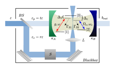
Figure 1: Pictorial representation of the experimental setup. An input field of strength $\varepsilon$ impinges on a beam splitter whose transmission and reflection coefficients are $t$ and $r$, respectively, and the reflected and transmitted beam are directed to a three-level atom inside an optical cavity. The transmitted part is used as a driving field $\varepsilon_{P}$ on the cavity mode, while the reflected part is used as the control field $\varepsilon_{c}$. A polarizer $S$ and a lens $L$ are placed in the way of the control field $\varepsilon_{c}$ to adjust its polarization and the Rabi frequency to properly interact with a specific atomic transition. The other parameters that appear in this figure are described in the main text. By increasing $\varepsilon$ we simultaneously increase the driving $\left(\varepsilon_{p}\right)$ and control $\left(\varepsilon_{c}\right)$ fields.

In this system a single three-level atom in a $\Lambda$ configuration has two ground states $\left|1\right\rangle$ and $\left|2\right\rangle$ and excited state $\left|3\right\rangle$. This three-level atom interacts with one mode of the optical cavity of frequency $\omega$ inducing $\left|1\right\rangle\leftrightarrow\left|3\right\rangle$ transitions with Rabi frequency $g$. In turn, the control field of frequency $\omega_{c}$ induces $\left|2\right\rangle\leftrightarrow\left|3\right\rangle$ transitions with Rabi frequency given by $\Omega_{c}=\frac{\mu\varepsilon_{c}}{\hbar}=r\mu\sqrt{\frac{\omega_{c}\left\langle n\right\rangle}{2\hbar\epsilon_{0}V_{c}}}$, where $V_{c}$ is the quantization volume regarded to the control field and can be diminished using a lens to focus the beam, $\epsilon_{0}$ is the vacuum permittivity, $\mu$ is the atomic dipole transition matrix element, and the average number of photons $\left\langle n\right\rangle$ of the input field. The Hamiltonian corresponding to the driving field onto the cavity mode impinging the optical cavity through the left wall is given by $\varOmega_{p}ae^{i\omega_{p}t}+h.c.$, where $h.c.$ stands for Hermitian conjugate, and $\varOmega_{p}=-i\sqrt{2\kappa_{A}}\varepsilon_{P}$ is the Rabi frequency for the probe field. Adopting state $\left|1\right\rangle$ as the zero energy level, the total Hamiltonian $H=H_{0}+H_{int}$ reads $\left(\hbar=1\right)$

$$H_{0}=\omega_{3}\sigma_{33}+\omega_{2}\sigma_{22}+\omega a^{\dagger}a,$$

$$H_{int}=ga\sigma_{31}+\Omega_{c}\sigma_{32}e^{-i\omega_{c}t}+\Omega_{p}ae^{i\omega_{p}t}+h.c.,$$

$$\sigma_{ij}=\left|i\right\rangle\left\langle j\right|,i,j=1,2,3.$$

In the interaction picture we can write this Hamiltonian as

$$H_{I}(t)=ga\sigma_{31}e^{i\Delta_{1}t}+\Omega_{c}\sigma_{32}e^{i\Delta_{c}t}+\Omega_{p}ae^{i\Delta_{p}t}+h.c,$$ (1)

where $\Delta_{1}\equiv\omega_{3}-\omega$, $\Delta_{c}\equiv\left(\omega_{3}-\omega_{2}\right)-\omega_{c}$, and $\Delta_{p}=\omega_{p}-\omega$ . The time-dependency of the interaction Hamiltonian Eq. (1) can be eliminated applying the unitary transformation $U_{1}=e^{-i\left[\Delta_{p}a^{\dagger}a-\Delta_{1}\sigma_{33}-\left(\Delta_{1}-\Delta_{c}\right)\sigma_{22}-\Delta_{p}\sigma_{11}\right]t}$, which allows us to rewrite this Hamiltonian as

$$\widetilde{H}_{I}=\Delta_{1}\sigma_{33}+(\Delta_{1}-\Delta_{c})\sigma_{22}+\Delta_{p}\sigma_{11}-\\ -\Delta_{p}a^{\dagger}a+\left[\Omega_{p}a+ga\sigma_{31}+\Omega_{c}\sigma_{32}+h.c.\right].$$ (2)

The master equation corresponding to Eq. (2) is

$$\frac{d\rho}{dt}=-i[\widetilde{H}_{I},\rho]+\kappa D\left[a\right]+\Gamma_{31}D\left[\sigma_{13}\right]+\\ +\Gamma_{32}D\left[\sigma_{23}\right]+\gamma_{2}D\left[\sigma_{22}\right]+\gamma_{3}D\left[\sigma_{33}\right],$$ (3)

where $\Gamma_{ij}$ is the atomic polarization decay rate from the state $\left|i\right\rangle\rightarrow\left|j\right\rangle$, $\gamma_{i}$ is the atomic dephasing of the state $\left|i\right\rangle$, $\kappa$ stands for the total cavity field decay rate, i.e., $\kappa=\kappa_{A}+\kappa_{B}$, and $D\left[A\right]=2A\rho A^{\dagger}-A^{\dagger}A\rho-\rho A^{\dagger}A$. We investigate the negative response of this system by solving the above master equation in the steady state regime. As this equation does not present analytical solution for arbitrary values of the parameters, we numerically solve it by using QuTip algorithms Qutip . In our simulations we are assuming a symmetric cavity, i.e., $\kappa_{A}=\kappa_{B}=\kappa/2$, $\kappa$ being our reference parameter and $\Gamma_{31}=\Gamma_{32}=\Gamma/2$. Since the dephasing rates of the levels $\left|2\right\rangle$ and $\left|3\right\rangle$ ($\gamma_{2}$ and $\gamma_{3}$) are usually very small as compared to the damping rates, we neglect them throughout this paper. Before presenting our main results, we stress that the Hamiltonian model above leads to the well known phenomena of electromagnetic induced transparency celso2010 ; Celso13 , as shown in Fig. 2, where the average photon number outgoing the cavity $\left\langle b_{out}^{\dagger}b_{out}\right\rangle/\kappa$ versus $\Delta_{p}/\kappa$ is shown. In this figure the solid (blue) line is for $\varepsilon=1.0\kappa$, the dashed (green) line is for $\varepsilon=2.0\kappa$, and the dotted (black) line is for $\varepsilon=3.0\kappa$. Note the central peak denoting the maximum of the transmission, which occurs for $\omega_{p}=\omega$. Also, note the secondary peaks, whose maxima are far apart from the center $\omega_{p}=\omega$ by $\pm\sqrt{ng^{2}+\Omega_{c}^{2}}$ where $n=1,2,...$ is the photon number of the eigenstates of the Hamiltonian given by Eq. (2), obtained considering all detunings and $\varOmega_{p}$ nulls Celso13 . These eigenstates, schematically shown in Fig. 3 (a), were explicitly derived in Ref. Celso13 . In Fig. 3 (b), the second order correlation function $g^{(2)}\left(0\right)$ (red dashed line), here divided by $100$ for convenience, the atomic absorption $\left|\mathbf{\text{Im}}\left\langle\sigma_{13}\right\rangle\right|$ (black dotted line), and the average photon number of the output field (solid blue line) are plotted as a function of the normalized average photon number $\left|\varepsilon/\kappa\right|^{2}$ of the input field. The parameters used were $\Gamma_{31}=\Gamma_{32}=\Gamma/2=\kappa/2$, $\Delta_{1}=\Delta_{c}=0$, $\Delta_{p}=1.1g$, $\Omega_{c}=8\varepsilon$, and $g=20\kappa$. Note that exactly on the maximum of the first peak, as seen from left to right, corresponding to the average photon number of the output state (solid blue curve), we see that the correlation function $g^{(2)}(0)$ (dashed red line) goes down close to zero, which indicates the predominance of the one-photon process. A similar behavior occurs for the second peak, where the maximum of the average photon number of the output practically coincides with a local minimum of the $g^{(2)}(0)$ function, indicating now a large contribution of the two-photon process.

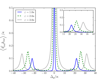
Figure 2: Average photon number transmission versus the normalized detuning between the probe and the cavity mode field ($\Delta_{P}/\kappa$) for different values of the driving field strength $\varepsilon$. The solid (blue) line is for $\varepsilon=1.0\kappa$, dashed (green) line is for $\varepsilon=2.0\kappa$, dotted (black) line is for $\varepsilon=3.0\kappa$. Here $g=20\kappa$ and $\Gamma=\kappa$.

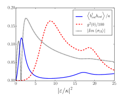
(a)	(b)

Figure 3: (a) Firsts eigenstates $\left({\scriptstyle\left|\psi_{n}^{\left(0\right)}\right\rangle},{\scriptstyle\left|\psi_{n}^{\left(\pm\right)}\right\rangle},n=0,1,2,...\right)$ of the Hamiltonian system given by Eq. (2), considering all detunings and $\varOmega_{p}$ nulls Celso13 . From this figure we can see that adjusting the Rabi frequency of control field $\Omega_{c}$ we can tune one or two (or even higher) photon resonances, as explained in the text. (b) Average photon number of the output field $\left\langle b_{out}^{\dagger}b_{out}\right\rangle/\kappa$ (blue solid line), correlation function $g^{(2)}\left(0\right)$, divided by $100$ for clarity (red dashed line), and the atomic absorption $\left|\text{\text{Im}}\left\langle\sigma_{13}\right\rangle\right|$ (black dotted line) as a function of the normalized input average photon number $\left|\varepsilon/\kappa\right|^{2}$.

Turning back to Fig. 2 and its inset, note that by increasing the strength of the driving field $\varepsilon$ the lateral peaks move away as both the driving $\left(\varepsilon_{P}\right)$ and the control $\left(\varepsilon_{c}\right)$ fields onto the cavity mode and the atom, respectively, depend directly on $\varepsilon$. As a consequence of this movement by the lateral peaks, the following effect can be seen: driving the system with a fixed detuning, for example $\Delta_{p}\simeq 22\kappa$, which is the detuning providing the maximum transmission for the blue solid line $\left(\varepsilon=1.0\kappa\right)$, we see that for larger values of the driving field $\left(\varepsilon\right)$, the transmission for this specific detuning goes down as the lateral peak moves to the right, as seen from the dash (green) and dot (black) curves at the same point.

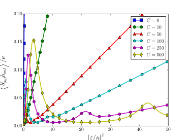
Figure 4: Average photon number of the output field versus normalized input field, $\left|\varepsilon/\kappa\right|^{2}$ for i) $C=0$ (square blue line); ii) $C=10$ (circle green line); iii) $C=50$ (triangle red line); iv) $C=100$ (pentagon aqua line); $C=250$ (hexagon violet line), and $C=500$ (diamond golden line). Here we used the following parameters: $\Gamma_{31}=\Gamma_{32}=\Gamma/2=\kappa/2$, $\Delta_{1}=\Delta_{c}=0$, $\Delta_{p}=1.1g$, and $\Omega_{c}=8\varepsilon$.

III Results

Now we investigate in details the negative response in this system. To be clear, we are going to increase the input field strength $\varepsilon$, thus simultaneously increasing both the control $\varepsilon_{c}$ and the driving $\varepsilon_{P}$ cavity fields, according to Fig. 1, in order to obtain a reduction in the output beam intensity.

Our main result is shown in Fig. 4, where we plot the output photon number average $\left\langle b_{out}^{\dagger}b_{out}\right\rangle/\kappa$ versus the rescaled input field intensity $\left|\varepsilon/\kappa\right|^{2}$ for several values of the cooperativity $C=g^{2}/(2\kappa\varGamma)$. Here we note that although we have used $t/r=4$, this ratio is not important to accomplish our proposal, since the control field Rabi frequency $\varOmega_{c}$ can be adjusted by simply focusing the reflected beam, once $\Omega_{c}$ is inversely proportional to the square root of the volume $V_{c}$ of the beam interacting with the atom. The parameters used here were $\Gamma_{31}=\Gamma_{32}=\Gamma/2=\kappa/2$, $\Delta_{1}=\Delta_{c}=0$, $\Delta_{p}=1.1g$, $\Omega_{c}=8\varepsilon$, $\varOmega_{p}=-0.8i\sqrt{\kappa_{A}}\varepsilon$, and $C$ ranges from $0$ to $500$. To these parameters we can see two peaks in Fig. 4, depending on the values of $C$, with the negative response starting at the maximum and ending at the subsequent minimum. As for example, for $C=250$ (hexagon violet line), negative response start in the first peak, as seen from the left to the right, around $\left|\varepsilon/\kappa\right|^{2}=2$, and finishes at $\left|\varepsilon/\kappa\right|^{2}=10$, starting again in the second peak, around $\left|\varepsilon/\kappa\right|^{2}=22$, finishing at $\left|\varepsilon/\kappa\right|^{2}=27$. Therefore, starting at the first peak as seen from the left, we see the transmission going down as we increase the strength of the driving field due to the movement to the right of the main peak. Then, the transmission increases again, since the system reaches a two-photon resonance, and subsequently it goes down. Finally, the transmission begins to increase to larger values of the input field as the atomic system saturates. For very large values of the input field, the average photon number inside the cavity increases linearly with $\left|\varepsilon/\kappa\right|^{2}$, whose behavior is identical to that of an empty cavity coherently driven (not shown in Fig. 4).

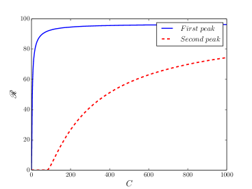
Figure 5: The parameter $\mathscr{R}$, a measure of negative response, gives the percentage of the output beam variation as a function of the cooperativity $C$. Here we plot $\mathscr{R}$ for both the one-photon resonance (first peak in solid blue line), and the two-photon resonance (second peak in red dashed line). Note that the maximum variation for both one- and -two photon resonances stabilize near of 95% (solid-blue line) and 80% (dashed-red line). Here, first peak (second peak) refers to the leftmost (rightmost) peak appearing in Fig. 4.

Since each cooperativity $C$ determines different negative responses, it is useful to define a parameter $\mathscr{R}$ that can be used in order to quantify the negative response in terms of the variation in the output beam intensity. Indeed, cooperativity $C$ giving rise to a very small negative response could be not attractive from the experimental point of view. We thus propose the parameter $\mathscr{R}=\frac{\left(\left\langle b_{out}^{\dagger}b_{out}\right\rangle_{max}-\left\langle b_{out}^{\dagger}b_{out}\right\rangle_{min}\right)}{\left\langle b_{out}^{\dagger}b_{out}\right\rangle_{max}}\times 100\%$ relating the maximum value taken by the output beam in the first (second) peak and the subsequent minimum right after the first (second) peak. In Fig. 5 we show this parameter, which gives the percentage of the output beam variation, as a function of the cooperativity $C$, for both the first (solid, blue line) and the second (dashed, red line) peaks. Note that the larger the parameter $\mathscr{R}$, the higher the percentage of the output beam variation, allowing the experimentalist to choose $C$ conveniently to guarantee that the negative response be evaluated or even optimized. Note that, to the parameters used here, $\mathscr{R}$ increases monotonically with the cooperativity, reaching the maximum around 95% for the one-photon resonance (solid-blue line) and around 80% for two-photon resonance (dashed-red line). Also, note that negative response for one-photon resonance (solid blue line), as measured by the $\mathscr{R}$ parameter, initiates at small values of the cooperativity $\left(C>0\right)$ and grows faster up to $C\simeq 60$, saturating after $C\sim 200$, while for two-photon resonances (dashed-red line), $\mathscr{\mathscr{R}}$ initiates at $C\simeq 85$, growing steadily and saturating for $C\sim 1000$. Interesting, to this case note that there is no negative response for cooperativity values lesser than $C\simeq 85$, no matter the intensity of the input field. This is due to the difficulty of having two-photon processes for small values of the cooperativity.

IV Conclusions

In this paper we have studied negative response in the context of optical cavity and traveling wave field. We presented an experimentally feasible scheme to observe decreasing of the output field intensity while increasing the intensity of the input field, therefore a negative response phenomenon. We characterize this negative response for a large range of atom-quantum field Rabi frequencies, and we were able to propose the parameter $\mathscr{R}$ that quantifies the efficiency of this effect through the percentage of the negative variation of the output field when the input field is positively varied. We also showed that negative response can be displayed to either one-photon and two-photon resonances, with one-photon resonance requiring lower values of the cooperativity. Among some applications, we pointed out that our proposal can be helpful to protect fragile devices against sudden variation of field intensities, such as field detectors sensitive to few photons. In particular, a device made with the principles developed here could be used to defeat the fake Bell violation strategy used elsewhere Scarani11 , which consists in impinging strong field intensity to blind single photon detectors, manipulating their outputs to simulate the arriving of a single photon in the detector that they choose conveniently.

- (1) A. Mari and J. Eisert, Phys. Rev. Lett. 108, 120602 (2012).
- (2) B. Cleuren, B. Rutten, and C. Van den Broeck, Phys. Rev. Lett. 108, 120603 (2012).
- (3) D. Z. Rossatto, A. R. de Almeida, T. Werlang, C. J. Villas-Boas, and N. G. de Almeida, Phys. Rev. A 86, 035802 (2012).
- (4) C. J. Villas-Boas, W. B. Cardoso, A. T. Avelar, A. Xuereb, and N. G. de Almeida, Quantum Inf Process (2016) 15:2021–2032.
- (5) M. J. Collett and C. W. Gardiner, Physical Review A 30, 1386 (1984).
- (6) S. Gleyzes et al., Nature (London) 446, 297 (2007).
- (7) J. M. Raimond, M. Brune, and S. Haroche, Rev. Mod. Phys. 73, 565 (2001).
- (8) E. Hinds and R. Blatt, Nature 492, 55 (2012), and references therein.
- (9) V. Makarov, New J. Phys. 11, 065003 (2009)
- (10) I. Gerhardt et al., Nature Comm. 2, 349 (2011)
- (11) Ilja Gerhardt et al., Phys. Rev. Lett. 107, 170404 (2011)
- (12) A. Acín, N. Gisin, and L. Masanes, Phys. Rev. Lett. 97,120405 (2006).
- (13) J.-D. Bancal, N. Gisin, Y.-C. Liang, and S. Pironio, Phys. Rev. Lett. 106, 250404 (2011).
- (14) S. Popescu and D. Rohrlich, Found. Phys. 24, 379 (1994).
- (15) M. Mucke et al., Nature 465, 755 (2010).
- (16) J. A. Souza, I. Figueiroa, H. Chibani, C. J. Villas-Boas, and G. Rempe, Phys. Rev. Lett. 111, 113602 (2013).
- (17) J. R. Johansson, P. D. Nation, F. Nori, Computer Physics Comm. 184, 1234 (2013).