[columns=3, title=Alphabetical Index]

Gane Samb Lo
Aladji Babacar Niang
Lois Chinwendu Okereke

A Course on Elementary Probability Theory

Statistics and Probability African Society (SPAS) Books Series.
Saint-Louis, Calgary, Alberta. 2020.

DOI : http://dx.doi.org/10.16929/sts/2020.001

ISBN: 9798582099772

Prof Gane Samb LO
gane-samb.lo@ugb.edu.sn, gslo@ugb.edu.ng
Gaston Berger University (UGB), Saint-Louis, SENEGAL.
African University of Science and Technology, AUST, Abuja, Nigeria.

Hamet Seydi.
Universités of SENEGAL.
hseydi@gmail.com

Brahim MEZERDI.
mezerdi@univ-biskra.dz, bmezerdi@yahoo.fr
Université Biskra, Algeria

Blaise SOME
some@univ-ouaga.bf
Chairman of LANIBIO, UFR/SEA
Ouaga I Pr Joseph Ki-Zerbo University.

Mohamed Ahsanullah
ahsan@rider.edu
Rider University, Lawrence, USA.

Dr Diam Ba
dba@statpas.org
Gaston Berger University, Senegal.

Tchilabalo Abozou KPANZOU
kpanzout@yahoo.fr, kpanzouta@statpas.org
Kara University, Togo.

List of published books

Collection : SPAS BOOKS SERIES.

1. A Collection of Papers in Mathematics and Related Sciences. Hamet SEYDI, Gane Samb LO, and Aboubakary DIAKHABY (eds.) (2018)
Doi : 10.16929/sbs/2018.100. ISBN: 978-2-9559183-0-2. Available at:
Euclid.org :https://projecteuclid.org/euclid.spaseds/1569509457 Amazon.com : Search COLLECTION-PAPERS-MATHEMATICS-RELATED-SCIENCES

For the latest updates, visit our official website :

www.statpas.org/spaseds/

Library of Congress Cataloging-in-Publication Data

Gane Samb LO, 1958-;
Aladji Babacar Niang 1994-; Lois Chinwendu Okereke 1989-

A Course on Elementary Probability Theory.

SPAS textbooks Series, 2020.

DOI : 10.16929/sts/2020.001

ISBN 9798576736386.

Author : Gane Samb LO

Emails:
gane-samb.lo@ugb.edu.sn, ganesamblo@ganesamblo.net, gslo@aust.edu.ng

Url’s:
www.ganesamblo@ganesamblo.net
www.statpas.net/@ganesamblo

Affiliations.
Main affiliation : University Gaston Berger, UGB, SENEGAL.
African University of Sciences and Technology, AUST, Abuja, Nigeria.
Affiliated as a researcher to : LSTA, Pierre et Marie Curie University, Paris VI, France.

Teaches or has taught at the graduate level in the following universities:
Saint-Louis, Senegal (UGB)
Abuja - Nigeria (AUST)
Banjul - Gambia (TUG)
Bamako - Mali (USTTB)
Ouagadougou - Burkina Faso (UJK)
African Institute of Mathematical Sciences, Mbour, SENEGAL, AIMS.
Franceville - Gabon
Kara, (Togo), undergraduate level

General acknowledgment.

As main author, I wish to acknowledge the help of many people. I have been working for almost thirty years, mainly at the Saint-Louis Gaston University, since 1991. I also taught in many African Universities, especially at the master degree level. I worked in the administration of the university at all levels (head of department, dean faculty, vice-president). I also supervised more than twenty Ph.D. theses and several master dissertations. As well, I animated the LERSTAD, a research group I created around 1992 and ran it for years with a regular weekly seminar.

The books I am writing are the outcomes of all these activities. I worked with amazing people, younger colleagues and Ph.D. students who became later high profiled researchers in Africa, Europa, Canada and the United States, and other parts of the world. For the last few years, I have been teaching in Nigeria, in the African University of Sciences and Technology of the Nelson Mandela Institute, Abuja, Nigeria.

The books of this series in Mathematics in general, and in Random Analysis (Probability Theory and Statistics and their applications) are written in English since we want to reach a bigger public. But French versions will be published for books regularly used in undergraduate education. A broader presentation of our series of book can be found in the general preface, in page General Preface.

I want to thank many people involved in the publication process of our books, particularly this one:

(1) Students who followed this course at Université Gaston Berger and at Université Dakar-Bourguiba (SENEGAL) during years. The course I taught them has become the book you have in your hand.

(2) Members of my research teams (LERSTAD, IMHOTEP) who are asked to read all our books and who regularly take part in the editing (Drs. Tchilabola A. Kpanzou [Togo]; Harouna Sangaré, Soumaila Dembél’é, Mouminou Diallo [Mali]; Modou Ngom, Diam Bâ, Amadou Dadhié Ba; Mrs Gorgui Gning, Cherif Mamadou Moctar Traoré, etc.)

(3) In 2018, my former students in Measure Theory and Integration in Abuja : Tagbo Innocent Aroh, Lois Chinwendu Okereke, Abubakar Adamu, Aicha Adam Aminu, Chidiebere Eze Leonard Eze, helped in polishing the English text and checked the mathematical formulas.

(4) My collaborators Aladji Babacar Niang and Lois Chinwendu Okereke, who conducted a thorough editing of the book. I am convinced that their work tremendously improved this book. As a result, I consider them co-authors with at least twenty-five percent of the co-authorship for each of them.

Acknowledgment of Funding.

The author acknowledges continuous and various support from the authorities of Gaston Berger University. It is true that in Senegalese public universities, the weekly teaching charge for full professors is five hours per week. The remaining time is devoted for supervision and research activities. Accordingly, scholars have all the means to realize their research activities : personal office, equipment with computers, printers, fax machines, ink, paper, internet connection, etc., and funding for participation in conferences.

In that sense, I acknowledge that writing the books of this series is implicitly funded by the university and the state of Senegal. I express my most sincere appreciations to their authorities.

Abstract of the book.

This book introduces to the theory of probabilities from the beginning. Assuming that the reader possesses the normal mathematical level acquired at the end of the secondary school, we aim to equip him with a solid basis in probability theory. The theory is preceded by a general chapter on counting methods. Then, the theory of probabilities is presented in a discrete framework. Two objectives are sought. The first is to give the reader the ability to solve a large number of problems related to probability theory, including application problems in a variety of disciplines. The second is to prepare the reader before he takes course on the mathematical foundations of probability theory. In this later book, the reader will concentrate more on mathematical concepts, while in the present text, experimental frameworks are mostly found. If both objectives are met, the reader will have already acquired a definitive experience in problem-solving ability with the tools of probability theory and at the same time he is ready to move on to a theoretical course on probability theory based on the theory of Measure and Integration. The book ends with a chapter that allows the reader to begin an intermediate course in mathematical statistics.

Keywords. combinatorics; discrete counting; elementary probability; equi-probability; events and operation on events; independence of events; conditional probabilities; Bayes’ rules; random variables; discrete and continuous random variables; bi-dimensional random variable; probability laws; probability density functions; cumulative distribution functions; Independence of random variables; usual probability laws and their parameters; introduction to statistical mathematics; convex functions; .

AMS 2010 Classification Subjects : 60GXX; 62GXX.

Résumé de l’ouvrage.

Cet ouvrage introduit à la théorie des probabilités depuis le début. En supposant que le lecteur possède le niveau mathématique normal acquis à la fin du lycée, nous ambitionnons de le doter d’une base solide en théorie des probabilités. L’exposé de la théorie est précédé d’un chapitre général sur les méthodes de comptage. Ensuite, la théorie des probabilités est présentée dans un cadre discret. Deux objectifs sont recherchés. Le premier est de donner au lecteur la capacité à résoudre un grand nombre de problèmes liés à la théorie des probabilités, y compris les problèmes d’application dans une variété de disciplines. Le second était de préparer le lecteur avant qu’il n’aborde l’ouvrage sur les fondements mathématiques de la théorie des probabilités. Dans ce dernier ouvrage, le lecteur se concentrera davantage sur des concepts mathématiques tandis que dans le présent texte, il se trouvent surtout des cadres expérimentaux. Si les deux objectifs sont atteints, le lecteur aura déjà acquis une expérience définitive en capacité de résolution de problèmes de la vie réelle avec les outils de la théorie des probabilités et en même temps, il est prêt à passer à un cours théorique sur les probabilités basées sur la théorie de la mesure et l’intégration. Le livre se termine par par un chapitre qui permet au lecteur de commencer un cours intermédiaire en statistiques mathématiques.

Dedication.

Figure 1. The ever smiling young lady

General Preface

This textbook is part of a series whose ambition is to cover broad part of Probability Theory and Statistics. These textbooks are intended to help learners and readers, both of of all levels, to train themselves.

As well, they may constitute helpful documents for professors and teachers for both courses and exercises. For more ambitious people, they are only starting points towards more advanced and personalized books. So, these texts are kindly put at the disposal of professors and learners.

Our textbooks are classified into categories.

A series of introductory books for beginners. Books of this series are usually accessible to student of first year in universities. They do not require advanced mathematics. Books on elementary probability theory and descriptive statistics are to be put in that category. Books of that kind are usually introductions to more advanced and mathematical versions of the same theory. The first prepare the applications of the second.

A series of books oriented to applications. Students or researchers in very related disciplines such as Health studies, Hydrology, Finance, Economics, etc. may be in need of Probability Theory or Statistics. They are not interested in these disciplines by themselves, rather in the need to apply the findings of these disciplines as tools to solve their specific problems. So adapted books on Probability Theory and Statistics may be composed to focus on the applications of such fields. A perfect example concerns the need of mathematical statistics for economists who do not necessarily have a good background in Measure Theory.

A series of specialized books on Probability theory and Statistics of high level. This series begin with a book on Measure Theory, its counterpart of probability theory, and an introductory book on topology. On that basis, we will have, as much as possible, a coherent presentation of branches of Probability theory and Statistics. We will try to make it self-contained, as much as possible, so that anything we need will be in the series.

Finally, research monographs close this architecture. The architecture should be so large and deep that the readers of monographs booklets will find all needed theories and inputs in it.

We conclude by saying that, with only an undergraduate level, the reader will open the door of anything in Probability theory and statistics with Measure Theory and integration. Once this course validated, eventually combined with two solid courses on topology and functional analysis, he will have all the means to get specialized in any branch in these disciplines.

Our collaborators and former students are invited to make live this trend and to develop it so that the center of Saint-Louis becomes or continues to be a renowned mathematical school, especially in Probability Theory and Statistics.

Preface of the first edition 2018

The current series of Probability Theory and Statistics are based on two introductory books for beginners : A Course of Elementary probability Theory and A course on Descriptive Statistics.

All the more or less advanced probability courses are preceded by this one. We strongly recommend you do not skip it. It has the tremendous advantage of making the feel reader the essence of probability theory by using extensively random experiences. The mathematical concepts come only after a complete description of a random experience.

This book introduces the theory of probabilities from the beginning. Assuming that the reader possesses the normal mathematical level acquired at the end of the secondary school, we aim to equip him with a solid basis in probability theory. The theory is preceded by a general chapter on counting methods. Then, the theory of probabilities is presented in a discrete framework.

Two objectives are sought. The first is to give the reader the ability to solve a large number of problems related to probability theory, including application problems in a variety of disciplines. The second is to prepare the reader before he approached the textbook on the mathematical foundations of probability theory. In this book, the reader will concentrate more on mathematical concepts, while in the present text, experimental frameworks are mostly found. If both objectives are met, the reader will have already acquired a definitive experience in problem-solving ability with the tools of probability theory and at the same time he is ready to move on to a theoretical course on probability theory based on the theory of measurement and integration.

The book ends with a chapter that allows the reader to begin an intermediate course in mathematical statistics .

I wish you a pleasant reading and hope receiving your feedback.

To my late and beloved sister Khady Kane Lo(1953- ).

Saint-Louis, Calgary, Abuja, Bamako, Ouagadougou, 2017.

Introduction

There exists a tremendous number of random phenomena in nature, real life and experimental sciences.

Almost everything is random in nature : whether, occurrences of rain and their durations, number of double stars in a region of the sky, lifetimes of plants, of humans, and of animals, life span of a radioactive atom, phenotypes of offspring of plants or any biological beings, etc.

The general theory states that each phenomena has a structural part (that is deterministic) and a random part (called the error or the deviation).

Randomness also appears as conceptual experiments : tossing a coin once or 100 times, throwing three dice, arranging a deck of cards, matching two decks, playing roulette, etc.

Every day human life is subject to randomness : waiting times for buses, traffic, number of calls on a telephone, number of busy lines in a communication network, sex of a newborn, etc.

The reader is referred to feller1 for a more diverse and rich set of examples.

The quantitative study of random phenomena is the objective of Probability Theory and Statistics Theory. Let us give two simple examples to briefly describe each of these two disciplines.

In Probability Theory, one assigns a chance of realization to a random event before its realization, taking into account the available information.

Example : A good coin, that is, a homogenous and well balanced, is tossed. Knowing that the coin cannot stand on its rim, there is a 50% chances of having a Tail .

We base our conclusion on the lack of any reason to favor one of the possible outcomes : head or tail. So we convene that these outcomes are equally probable and then get 50% chances for the occurring for each of them.

Let us start with an example. Suppose that we have a coin and we do not know any thing of the material structure of the coin. In particular, we doubt that the coin is homogenous .

We decide to toss it repeatedly and to progressively monitor the occurring frequency of the head. We denote by $N_{n}$ the number of heads obtained after $n$ tossing and define the frequency of the heads by

$$F_{n}=\frac{N_{n}}{n}.$$

It is conceivable to say that the stability of $F_{n}$ in the neighborhood of some value $p\in]0,1[$ is an important information about the structure of the coin.

In particular, if we observe that the frequency $F_{n}$ does not deviate from $p=50\%$ more than $\varepsilon=0.001$ whenever $n$ is greater than $100$, that is

$$\left|F_{n}-1/2\right|\leq 10^{-3}$$

for $n\geq 100$, we will be keen to say that the probability of occurrence of the head is $p=50\%$ and, by this, we accept that that the coin is fair.

Based on the data (also called the statistics), we have estimated the probability of having a head at $p=50\%$ and accepted the pre-conceived idea (hypothesis) that the coin is good in the sense of homogeneity.

The reasoning we made and the method we applied are perfect illustrations of Statistical Methodology : estimation and model or hypothesis validation from data.

In conclusion, Statistics Theory enables the use of the data (also called statistics or observations), to estimate the law of a random phenomenon and to use that law to predict the future of the same phenomenon (inference) or to predict any other phenomenon that seems identical to it (extrapolation).

(1) The discipline of Statistics Theory and that of Probability Theory are two ways of treating the same random problems.

(2) The first is based primarily on the data to draw conclusions .

(3) The second is based on theoretical, and mathematical considerations to establish theoretical formulas.

(4) Nevertheless, the Statistics discipline may be seen as the culmination of Probability Theory .

This book is an introduction to Elementary Probability Theory. It is the result of many years of teaching the discipline in Universities and High schools, mainly in Gaston Berger Campus of Saint-Louis, SENEGAL.

It is intended to those who have never done it before. It focuses on the essential points of the theory. It is particularly adapted for undergraduate students in the first year of high schools.

The basic idea of this book consists of introducing Probability Theory, and the notions of events and random variables in discrete probability spaces. In such spaces, we discover as much as possible at this level, the fundamental properties and tools of the theory.

So, we do not need at this stage the elaborated notion of $\sigma$-algebras or fields. This useful and brilliant method has already been used, for instance, in Billingsley billingsleyMT for deep and advanced probability problems.

The book will finish by a bridge chapter towards a medium course of Mathematical Statistics. In this chapter, we use an analogy method to express the former results in a general shape, that will be the first chapter of the a fore mentioned course.

The reader will have the opportunity to master the tools he will be using in this course, with the coming course on the mathematical foundation of Probability Theory, which will be an element of our Probability and Statistics series. For such an advanced course, still to come, the reader will have to get prepared by a course of Measure Theory of Integration.

In this computer dominated world, we are lucky to have very powerful and free software like R and Scilab, to cite only the most celebrated. We seized this tremendous opportunity to use numerical examples using R software throughout the text.

The remainder of the book is organized as following.

Chapter 1 is a quick but sufficient introduction to combinatorial analysis. The student interested in furthering knowledge in this subject can refer to the course on general algebra.

Chapter 2 is devoted to an introduction to probability measures in discrete spaces. The notion of equi-probability is also dealt with, there.

Conditional probability and independence of random events are addressed in Chapter 3.

Chapter 4 introduces random variables, and presents a review of the usual probability law s.

Chapter 5 is devoted to the computations of the parameters of the usual laws. Mastering the results of this chapter and those in Chapter 4 is in fact of great importance for higher level courses.

A window on dependence methods will be presented in Chapter 6.

Distribution functions of random variables are studied in Chapter 7, which introduces continuous random variable s.

Chapter 1 Elements of Combinatorics

Here, we are concerned with counting cardinalities of subsets of a reference set $\Omega$, by following specific rules. We begin by a general counting principle.

The cardinality of a set $E$ is the number of its elements, denoted by $Card(E)$ or $\#(E)$. For an infinite set $E$, we have

$$Card(E)=\#(E)=+\infty.$$

Let us consider the following example : A student has two (2) skirts and four (4) pants in his closet. He decides to pick at random a skirt and pants to dress. In how many ways can he dress by choosing a skirt and pants? Surely, he has 2 choices for a skirt and for each of these choices, he has four possibilities to pick pants. In total, he has

$$2\times 4$$

ways to dress.

We applied the following general counting principle.

Proposition 2.1. Suppose that the set $\Omega$ of size $n$ can be partitioned into $n_{1}$ subsets $\Omega_{i}$, $i=1,...,n_{1}$ of same size; and that each of these subsets $\Omega_{i}$ can be split into $n_{2}$ subsets $\Omega_{ij}$, j = 1, . . ., $n_{2}$, $i=1,...,n_{1}$, of same size, and that each of the $\Omega_{ij}$ can be divided into $n_{3}$ subsets $\Omega_{ijh}$, $h=1,...,n_{3}$, $j=1,...,n_{2}$, $i=1,...,n_{1}$ of same size also. Suppose that we may proceed like that up an order $k$ with $n_{k}$ subsets with common size $a$.

Then the cardinality of $\Omega$ is given by

$$n=n_{1}\times n_{2}\times\times...\times n_{k}\times a.$$

Proof. Denote by $B_{h}$ the cardinality of a subset generated at step $h$, for $h=0,...,k$. A step $h$, we have $n_{h}$ subsets partitioned into $n_{h+1}$ subsets of same size. Then we have

$$B_{h}=n_{h+1}\times B_{h+1}\text{ for all }0\leq h\leq k-1,$$

with $B_{0}=n$, $B_{k+1}=a$. Now, the proof is achieved by induction in the following way

$$n = B_{0}=n_{1}\times B_{1}$$

$$= n_{1}\times n_{2}B_{2}$$

$$= n_{1}\times n_{2}\times n_{3}B_{3}$$

$$...$$

$$= n_{1}\times n_{2}\times n_{3}\times....\times n_{k}\times B_{k},$$

with $B_{k}=a$.

Although this principle is simple, it is a fundamental tool in combinatorics : divide and count.

But it is not always applied in a so simple form. Indeed, partitioning is the most important skill to develop in order to apply the principle successfully.

This is what we will be doing in all this chapter.

Let $E$ be a set of $n$ elements with $n\geq 1$.

Definition 2.1. A $p$-tuple of $E$ is an ordered subset of $E$ with $p$ distinct elements of $E$. A $p$-tuple is called a $p$-permutation or $p$-arrangement of elements of $E$ and the number of $p$-permutations of elements of $E$ is denoted as $A_{n}^{p}$ (we read $p$ before $n$). It is also denoted by

$$(n)_{p}.$$

We have the result.

Theorem 2.1. For all $1\leq p\leq n$, we have

$$A_{n}^{p}=n(n-1)(n-2)......(n-p+1).$$

Proof. Set $E=\left\{x_{1},...,x_{n}\right\}$. Let $\Omega$ be the class of all ordered subsets of $p$ elements of $E$. We are going to apply the counting principle to $\Omega$.

It is clear that $\Omega$ may be divided into $n=n_{1}$ subsets $F_{i}$, where each $F_{i}$ is the class of ordered subsets of $\Omega$ with first elements $x_{i}$. Since the first element is fixed to $x_{i}$, the cardinality of $F_{i}$ is the number of ordered subsets of $E\setminus\{x_{i}\}$, so that the classes $F_{i}$ have a common cardinality which is the number of $(p-1)$-permutations from a set of $(n-1)$ elements. We have proved that

(1.0.1) $$A_{n}^{p}=n\times A_{n-1}^{p-1},$$

for any $1\leq p\leq n$. We get by induction

$$A_{n}^{p}=n\times(n-1)\times A_{n-2}^{p-2}$$

and after $h$ repetitions of (1.0.1), we arrive at

$$A_{n}^{p}=n\times(n-1)\times(n-2)\times...\times(n-h)\times A_{n-h-1}^{p-h-1}.$$

For $h=p-2$, we have

$$A_{n}^{p}=n\times(n-1)\times(n-2)\times...\times(n-p+2)\times A_{n-p+1}^{1}.$$

And, clearly, $A_{n-p+1}^{1}=n-p+1$ since $A_{n-p+1}^{1}$ is the number of singletons form a set of $(n-p+1)$ elements.

Remark. Needless to say, we have $A_{n}^{p}=0$ for $p\geq n+1$.

Here are some remarkable values of $A_{n}^{p}$. For any positive integer $n\geq 1$, we have

(i) $A_{n}^{0}=1$.

(ii) $A_{n}^{1}=n$.

From an algebraic point of view, the numbers $A_{n}^{p}$ also count the number of injections.

We begin by recalling the following algebraic definitions :

A function from a set $E$ to a set $F$ is a correspondence from $E$ to $F$ such that each element of $E$ has at most one image in $F$.

A mapping from a set $E$ to a set $F$ is a correspondence from $E$ to $F$ such that each element of $E$ has exactly one image in $F$.

An injection from a set $E$ to a set $F$ is a mapping from $E$ to $F$ such that each any two distinct elements of $E$ have distinct images in $F$.

A surjection from a set $E$ to a set $F$ is a mapping from $E$ to $F$ such that each element of $F$ is the image of at least one element of $E$.

A bijection from a set $E$ onto a set $F$ is a mapping from $E$ to $F$ such that each element of $F$ is the image of one and only element of $E$.

If there is an injection (respectively a bijection) from $E$ to $F$, then we have the inequality: $Card(E)\leq Card(F)$ (respectively, the equality $Card(E)=Card(F)$).

The number of $p$-arrangements from $n$ elements ($p\leq n$) is the number of injections from a set of $p$ elements to a set of $n$ elements.

The reason is the following. Let $E=\{y_{1},...,y_{p}\}$ and $F=\{x_{1},x_{2,}...,x_{n}\}$ be sets with $Card(E)=p$ and $Card(F)=n$ with $p\leq n$. Forming an injection $f$ from $E$ on $F$ is equivalent to choosing a $p$-tuple $(x_{i_{1}}...x_{i_{p}})$ in $F$ and to set the following correspondence $f(y_{h})=x_{i_{h}}$, $h=1,...,p$. So, we may find as many injections from $E$ to $F$ as $p$-permutations of elements of from $F$.

Thus, $A_{n}^{p}$ is also the number of injections from a set of $p$ elements on a set of $n$ elements.

The number of mappings from a set of $p$ elements to a set of $n$ elements is $n^{p}$.

Indeed, let $E=\{y_{1},...,y_{p}\}$ and $F=\{x_{1},x_{2,}...,x_{n}\}$ be sets with $Card(E)=p$ and $Card(F)=n$ with no relation between $p$ and $n$. Forming a mapping $f$ from $E$ on $F$ is equivalent to choosing, for any $x\in E$, one arbitrary element of $F$ and to assign it to $x$ as its image. For the first element $x_{1}$ of $E$, we have $n$ choices, $n$ choices also for the second $x_{2}$, $n$ choices also for the third $x_{3}$, and so forth. In total, we have choices to form a mapping from $E$ to $F$.

Example on vote casting in Elections. The $p$ members of some population are called to mandatory cast a vote for one of $n$ candidates at random. The number of possible outcomes is the number of injections from a set of $p$ elements to a set of $n$ elements : $n^{p}$.

Definition 2.2. A permutation or an ordering of the elements of $E$ is any ordering of all its elements. If $n$ is the cardinality of $E$, the number of permutations of the element of $E$ is called : n factorial, and denoted $n!$ (that is $n$ followed with an exclamation point).

Before we give the properties of n factorial, we point out that a permutation of $n$ objects is a $n$-permutation of $n$ elements.

Theorem 2.2. For any $n\geq 1$, we have

(i) $n!=n(n-1)(n-2)......2\times 1$.

(ii) $n!=n(n-1)!$.

Proof. By remembering that a permutation of $n$ objects is an $n$-permutation of $n$ elements, we may see that Point (i) is obtained for $p=n$ in the Formula of Theorem 2.1. Point (ii) obviously derives from (i) by induction.

Exercise 2.1. What is the number of bijections between two sets of common cardinalily $n\geq 1$?

Exercise 2.2. Check that for any $1\leq p\leq n$,

$$A_{n}^{p}=n!/(n-p)!.$$

Let $\mathcal{E}$ be collection of $n$ distinct objects. Suppose that $\mathcal{E}$ is partitioned into $k$ sub-collections $\mathcal{E}_{j}$ of respective sizes $n_{1}$, . . .$n_{k}$ the following properties apply :

(i) Two elements of same sub-collection are indistinguishable between them.

(ii) Two elements from two different sub-collections are distinguishable one from the other.

What is the number of permutations of $\mathcal{E}$? Let us give an example.

Suppose we have $n=20$ balls of the same form (not distinguishable by the form, not at sight nor by touch), with $n_{1}=6$ of them of red color, $n_{2}=9$ of blue color and $n_{3}=5$ of green color. And we can distinguish them only by their colors. In this context, two balls of the same color are the same for us, from our sight. An ordering of these $n$ balls in which we cannot distinguish the balls of same color is called a permutation with repetition or a visible permutation.

Suppose that we have realized a permutation of these $n$ balls. Permuting for example only red balls between them does not change the appearance of the global permutation. Physically, it has changed but not visibly meaning from our sight. Such a permutation may be described as visible, or permutation with repetition.

In fact, any of the $n!$ real permutations represents all the visible repetitions where the $6$ red balls are permuted between them, the $9$ blue balls are permuted between them and the $5$ green balls are permuted between them. By the counting principle, a real permutation represents exactly

$$9!\times 6!\times 5!$$

permutations with repetition. Hence, the number of permutations with repetition of these $20$ balls is

$$\frac{20!}{9!\times 6!\times 5!}.$$

Now, we are going to do the same reasoning in the general case.

As we said before, we have two types of permutations here :

(a) The real or physical permutations, where the $n$ elements are supposed to be distinguishable.

(b) The permutations with repetition in which we cannot distinguish between the elements of a same sub-collection.

Theorem 2.3. The number of permutations with repetition of a collection $\mathcal{E}$ of $n$ objects partitioned into $k$ sub-collections $\mathcal{E}_{i}$ of size $n_{i}$, $i=1,...,k$, such that only elements from different sub-collections are distinguishable between them, is given by

$$B(n_{1},n_{2},...,n_{k})=\frac{n!}{n_{1}!n_{2}!......n_{k}!}.$$

Terminology. The numbers of permutations with repetition are also called multinomial coefficients, in reference Formula (1.0.6).

Proof. Let $B(n_{1},n_{2},...,n_{k})$ be the number of permutations with repetition. Consider a fixed real permutation. This real permutation corresponds exactly to all permutations with repetition obtained by permuting the $n_{1}$ objects of $\mathcal{E}_{1}$ between them, the $n_{2}$ objects of $\mathcal{E}_{2}$ between them, $\cdots$, and the $n_{k}$ objects of $\mathcal{E}_{k}$ between them. And we obtain $n_{1}!n_{2}!......n_{k}!$ permutations with repetition corresponding to the same real permutation. Since this is true for any real permutation which generates

$$n_{1}!\times n_{2}!\times...\times n_{k}!$$

visible permutations, we get that

$$(n_{1}!n_{2}!.....n_{k}!)\times B(n_{1},n_{2},...,n_{k})=n!.$$

This gives the result in the theorem.

Let us define the numbers of combinations as follows.

Definition 2.3. Let $E$ be a set of $n$ elements. A combination of $p$ elements of $E$ is a subset of $E$ of size $p$.

In other words, any subset $F$ of $E$ is a $p$-combination of elements of $E$ if and only if $Card(F)=p$.

It is important to remark that we can not have combinations of more that $n$ elements in a set of $n$ elements.

We have :

Theorem 2.4. The number of combinations of $p$ elements from $n$ elements is given by

$$\left(\begin{tabular}[]{c}$n$\\ $p$\end{tabular}\right)=\frac{n!}{p!(n-p)!}.$$

Proof. Denote by

$$\left(\begin{tabular}[]{c}$n$\\ $p$\end{tabular}\right)$$

the number of combinations of $p$ elements from $n$ elements.

The collection of $p$-permutations is exactly obtained by taking all the orderings of the elements of the combinations of $p$ elements from $E$. Each combination gives $p!$ $p$-permutations of $E$. Hence, the cardinality of the collection of $p$-permutations is exactly $p!$ times that of the class of $p$-combinations of $E$, that is

$$p!\text{ }\left(\begin{tabular}[]{c}$n$\\ $p$\end{tabular}\right)=A_{n}^{p}.$$

By using Exercise 2.1 above, we have

$$\left(\begin{tabular}[]{c}$n$\\ $p$\end{tabular}\right)=\frac{A_{n}^{p}\text{ }}{p!}=\frac{n!\text{ }}{\text{ }p!(n-p)!.}.$$

We also have this definition :

Definition 2.4. The numbers $\left(\begin{tabular}[]{c}$n$\\ $p$\end{tabular}\right)$, are also called binomial coefficients because of Formula (1.0.5) below.

The urn model plays a very important role in discrete Probability Theory and Statistics, especially in sampling theory. The simplest example of urn model is the one where we have a number of balls, distinguishable or not, of different colors.

We are going to apply the concepts seen above in the context of urns.

Suppose that we want to draw $r$ balls at random from an urn containing $n$ balls that are distinguishable by touch (where touch means hand touch).

We have two ways of drawing.

(i) Drawing without replacement. This means that we draw a first ball and we keep it out of the urn. Now, there are $(n-1)$ balls in the urn. We draw a second and we have $(n-2)$ balls left in the urn. We repeat this procedure until we have the $p$ balls. Of course, $p$ should be less or equal to $n$.

(ii) Drawing with replacement. This means that we draw a ball and take note of its identity or its characteristics (that are studied) and put it back in the urn. Before each drawing, we have exactly $n$ balls in the urn. A ball can be drawn several times.

It is clear that the drawing model (i) is exactly equivalent to the following one :

(i-bis) We draw $p$ balls at the same time, simultaneously, at once.

Now, we are going to see how the $p$-permutations and the $p$-combinations occur here, by a series of questions and answers.

Questions. Suppose that an urn contains $n$ distinguishable balls. We draw $p$ balls. In how many ways can the drawing occur? Or what is the number of possible outcomes in term of subsets formed by the $p$ drawn balls?

Solution 1. If we draw the $p$ balls without replacement and we take into account the order, the number of possible outcomes is the number of $p$-permutation s.

Solution 2. If we draw the $p$ balls without replacement and we do not take the order into account or there is no possible ordering, the number outcomes is the number of $p$-combinations from $n$.

Solution 3. If we draw the $p$ balls with replacement, the number of outcomes is $n^{p}$, the number of mapping s.

Needless to say, the ordering is always assumed if we proceed by a drawing with replacement.

Please, keep in mind these three situations that are the basic keys in Combinatoric s.

Now, let us explain the solutions before we continue.

Proof of Solution 1. Here, we draw the $p$ balls one by one. We have $n$ choices for the first ball. Once this ball is out, we have $(n-1)$ remaining balls in the urn and we have $(n-1)$ choices for the second ball. Thus, we have

$$n\times(n-1)$$

possible outcomes to draw two ordered balls. For three balls, $p=3$, we have the number

$$n\times(n-1)\times(n-2).$$

Remark that for $p=1,2,3$, the number of possible outcomes is

$$n\times(n-1)\times(n-2)\times....\times(n-p+1)=A_{n}^{p}.$$

You will not have any difficulty to get this by induction.

Proof of Solution 2. Here, there is no ordering. So we have to divide the number of ordered outcomes $A_{n}^{p}$ by $p!$ to get the result.

Proof of Solution 3. At each step of the $p$ drawing, we have $n$ choices. At the end, we get $n^{p}$ ways to draw $p$ elements.

We are going to devote a special subsection to the numbers of combinations or binomial coefficient s.

Here, we come back to the number of combinations that we call Binomial Coefficients here. First, let us state their main properties.

Main Properties.

Proposition 2.1. We have
(1) $\left(\begin{tabular}[]{c}$n$\\ $0$\end{tabular}\right)=1$ for all $n\geq 0$.
(2) $\left(\begin{tabular}[]{c}$n$\\ $1$\end{tabular}\right)=n$ for all $n\geq 1$.
(3 $\left(\begin{tabular}[]{c}$n$\\ $p$\end{tabular}\right)=\left(\begin{tabular}[]{c}$n$\\ $n-p$\end{tabular}\right)$, for $0\leq p\leq n$.
(4) $\left(\begin{tabular}[]{c}$n-1$\\ $p-1$\end{tabular}\right)+\left(\begin{tabular}[]{c}$n-1$\\ $p$\end{tabular}\right)=\left(\begin{tabular}[]{c}$n$\\ $p$\end{tabular}\right)$, for all $1\leq p\leq n$.

Proof. Here, we only prove Point (4). The other points are left to the reader as exercises.

$$\left(\begin{tabular}[]{c}$n-1$\\ $p-1$\end{tabular}\right)+\left(\begin{tabular}[]{c}$n-1$\\ $p$\end{tabular}\right) = \left\{\frac{(n-1)!}{(p-1)!(n-p)!}\right\}+\left\{\frac{(n-1)!}{p!(n-p-1)!}\right\}$$

$$= p\left\{\frac{(n-1)!}{p!(n-p)!}\right\}+(n-p)\left\{\frac{(n-1)!}{p!(n-p)!}\right\}$$

$$= \left\{\frac{(n-1)!}{p!(n-p)!}\right\}\left\{p+n-p\right\}$$

$$= \frac{n(n-1)!}{p!(n-p)!}$$

$$= \frac{n!}{p!(n-p)!}=\left(\begin{tabular}[]{c}$n$\\ $p$\end{tabular}\right).\ \ QED$$

Pascal’s Triangle. We are going to reverse the previous way by giving some of these properties as characteristics of the binomial coefficients. We have

Proposition 2.3. The formulas (i) and (ii):

(i) $\left(\begin{tabular}[]{c}$n$\\ $0$\end{tabular}\right)=\left(\begin{tabular}[]{c}$n$\\ $n$\end{tabular}\right)=1$ for all $n\geq 0$;
(ii) $\left(\begin{tabular}[]{c}$n-1$\\ $p-1$\end{tabular}\right)+\left(\begin{tabular}[]{c}$n-1$\\ $p$\end{tabular}\right)=\left(\begin{tabular}[]{c}$n$\\ $p$\end{tabular}\right)$, for all $1\leq p\leq n$

entirely characterize the binomial coefficient s

$$\left(\begin{tabular}[]{c}$n$\\ $p$\end{tabular}\right),\ \ 1\leq p\leq n.$$

Proof. We give the proof by using Pascal’s triangle. Point (ii) gives the following clog rule (règle du sabot in French)

n / p p-1 p

n-1 $$\left(\begin{tabular}[]{c}$n-1$\\ $p-1$\end{tabular}\right)$$

n

or more simply

$$u$$

With that rule, we may construct the Pascal’s triangle of the numbers $\left(\begin{tabular}[]{c}$n$\\ $p$\end{tabular}\right)$.

$$n/p$$ 0 1 2 3 4 5 6 7 8

0 1

1 1=u 1=v

2 1 1

3 1 3 3 1

4 1 4=u 6=v 4 1

5 1 5 10 5 1

6 1 1

7 1 1

8 1 1

The reader is asked to continue to fill this triangle himself. Remark that filling the triangle only requires the first column ($n=0$), the diagonal ($p=n$) and the clog rule. So points (i) and (ii) are enough to determine all the binomial coefficients. This leads to the following conclusion.

Proposition 2.4. Any array of integers $\beta(p,n)$, $0\leq p\leq n$ such that

(i) $\beta(n,n)$=$\beta(0,n)$= 1, for all $n\geq 0$,

(ii) $\beta(p-1,n-1)+\beta(p,n-1)=\beta(p,n),$ for 1 $\leq p\leq n$.

is exactly the array of binomial coefficients, that is

$$\beta(p,n)=\left(\begin{tabular}[]{c}$n$\\ $p$\end{tabular}\right),\ \ 0\leq p\leq n.$$

We are going to visit the Newton’s formula .

The Newton’s Formula .

Let us apply the result just above to the power $n$ of a sum of two scalars in a commutative ring ($\mathbb{R}$ for example).

Theorem 1.

For any $(a,b)\in\mathbb{R}^{2}$, for any $n\geq 1$, we have

(1.0.4) $$(a+b)^{n}=\sum_{p=0}^{n}\ \left(\begin{tabular}[]{c}$n$\\ $p$\end{tabular}\right)a^{p\ }b^{n-p}.$$

Proof. Since $\mathbb{R}$ is a commutative ring, we know that $(a+b)^{n}$ is a polynomial in $a$ and $b$ and it is written as a linear combination of terms $a^{p}\times b^{n-p}$, $p=0$,…,$n$. We have the formula

(1.0.5) $$(a+b)^{n}=\sum_{p=0}^{n}\ \beta(p,\ n)\ a^{p\ }b^{n-p}.$$

It will be enough to show that the array $\beta(p,\ n)$ is actually that of the binomial coefficients. To begin, we write

$$(a+b)^{n}=(a+b)\times(a+b)\times...\times(a+b).$$

From there, we see that $\beta(p,n)$ is the number of choices of $a$ or $b$ in each factor $(a+b)$ such that $a$ is chosen $p$ times and $b$ is chosen $(n-p)$ times. Thus $\beta(n,\ n)=1$ since $a^{n}$ is obtained in the unique case where $a$ is chosen in each factor $(a+b)$. Likely $\beta(0,\ n)=1$, since this corresponds to the monomial $b^{n}$, that is the unique case where $b$ is chosen in each case. So, Point (i) is proved for the array $\beta(\cdot,\cdot)$. Next, we have

$$(a+b)^{n} = (a+b)(a+b)^{n-1}$$

$$= (a+b)\times\sum_{p=0}^{n-1}\ \beta(p,\ n-1)a^{p}\ b^{n-p-1}$$

$$= (a+b)\left(\cdots+\beta(p-1,\ n-1)\ a^{p-1}b^{n-p}\right.$$

$$+ \left.\cdots+\beta(p,\ n-1)a^{p}\ b^{n-p-1}+\cdots\right)$$

This means that, when developing $(a+b)(a+b)^{n-1}$, the term $a^{p}\times b^{n-p}$ can only come out

(1) either from the product of $b$ by $a^{p}\times b^{n-p-1}$ of the binomial $(a+b)^{n-1}$,

(2) or from the product of $a$ by $a^{p-1}\times b^{n-p}$ of the binomial $(a+b)^{n-1}$.

Then we see that for $\leq p\leq n$, we get

$$\beta(p-1,\ n-1)+\beta(p,\ n-1)=\beta(p,\ n).$$

We conclude that the array $\beta(p,n)$ fulfills Points (i) and (ii) above. Then, this array is that of the binomial coefficients. QED.

Remark. The name of binomial coefficients comes from this Newton’s formula .

Multiple Newton’s Formula .

We are going to generalize the Newton’s Formula from dimension $k=2$ to an arbitrary dimension $k\geq 2$. Then binomial coefficients will be replaced by the numbers of permutations with repetition.

Let $k\geq 2$ and let us be given real numbers $a_{1}$,$a_{2}$, …, and $a_{k}$ and let $n\geq 1$ be a positive number. Consider

$$\Gamma_{n}=\{(n_{1},...,n_{k}),n_{1}\geq 0,...,n_{k}\geq 0,n_{1}+...+n_{k}=n\}.$$

We have

(1.0.6) $$(a_{1}+...+a_{k})^{n}=\sum_{(n_{1},...,n_{k})\in\Gamma_{n}}\frac{n!}{(n_{1}!\times n_{2}!\times...\times n_{k}!)}a_{1}^{n_{1}}\times a_{2}^{n_{2}}\times...\times a_{k}^{n_{k}},$$

that we may write in a more compact manner in

(1.0.7) $$\left(\sum_{i=1}^{k}a_{i}\right)^{n}=\sum_{(n_{1},...,n_{k})\in\Gamma_{n}}\frac{n!}{\prod_{i=1}^{k}n_{i}!}\prod_{i=1}^{k}a_{i}^{n_{i}}.$$

We will see how this formula is important for the multinomial law, which in turn is so important in Statistics .

Proof. Let us give a simple proof of it.

To develop $(\sum_{i=1}^{k}a_{i})^{n}$, we have to multiply $(\sum_{i=1}^{k}a_{i})$ by itself $n$ times. By the distributivity of the sum with respect to the product, the result will be a sum of products

$$z_{1}\times z_{2}\times...\times z_{n},$$

where each $z_{i}$ is one of the $a_{1}$, $a_{2}$, …, $a_{k}$. By commutativity, each of these products is of the form

(1.0.8) $$a_{1}^{n_{1}}\times a_{2}^{n_{1}}\times...\times a_{k}^{n_{k}},$$

where $(n_{1},...,n_{k})\in\Gamma_{n}$. And for a fixed $(n_{1},...,n_{k})\in\Gamma_{n}$, the product (1.0.8) is the same as all products

$$z_{1}\times z_{2}\times...\times z_{n},$$

in which we have $n_{1}$ of the $z_{i}$ identical to $a_{1}$, $n_{2}$ identical to $a_{2}$, …, and $n_{k}$ identical to $a_{k}$. These products correspond to the permutations with repetition of $n$ elements such that $n_{1}$ are identical, $n_{2}$ are identical, …, and $n_{k}$ are identical. Then, each product (1.0.8) occurs

$$\frac{n!}{(n_{1}!\times n_{2}!\times...\times n_{k}!)}$$

times in the expansion. This puts an end to the proof.

The number $n!$ grows and becomes huge very quickly. In many situations, it may be handy to have an asymptotic equivalent formula.

This formula is the Sterling’s one and it is given as follows :

$$n!=(2\pi n)^{\frac{1}{2}}\ \left(\frac{n}{e}\right)^{n}\ \exp(\theta_{n}),$$

with, for any $\eta>0$, for $n$ large enough,

$$\ \left|\theta_{n}\right|\leq\frac{1+\eta}{12n}.$$

This implies, in particular, that

$$n!\sim(2\pi n)^{\frac{1}{2}}\ \left(\frac{n}{e}\right)^{n},$$

as $n\ \rightarrow\ \infty$.

One can find several proofs (See feller1 , page 52, for example). In this textbook, we provide a proof in the lines of the one in valiron , pp. 167, that is based on Wallis integrals. This proof is exposed in Chapter 8 (which is an appendix), Section LABEL:proba01_appendix_stirling.

We think that a student in first year of University will be interested by an application of the course on Riemann integration.

Chapter 2 Introduction to Probability Measures

Assume that we have a perfect die whose six faces are numbered from $1$ to $6$. We want to toss it twice. Before we toss it, we know that the outcome will be a couple $(i,j)$, where $i$ is the number that will appear first and $j$ the second.

We always keep in mind that, in probability theory, we will be trying to give answers about events that have not occurred yet. In the present example, the possible outcomes form the set

$$\Omega=\left\{1,2,...,6\right\}\times\left\{1,2,...,6\right\}=\left\{(1,1),(1,2),...,(6,6)\right\}.$$

$\Omega$ is called the sample space of the experiment or the probability space. Here, the size of the set $\Omega$ is finite and is exactly $36$. Parts or subsets of $\Omega$ are called events. For example,

(1) {(3, 4)} is the event : Face 3 comes out in the first tossing and Face 4 in the second,

(2) A = $\left\{(1,1),(1,2),(1,3),(1,4),(1,5),(1,6)\right\}$ is the event : 1 comes out in the first tossing .

Any element of $\Omega$, as a singleton, is an elementary event. For instance $\{(1,1)\}$ is the elementary event : Face 1 appears in both tossing .

In this example, we are going to use the perfectness of the die, and the regularity of the geometry of the die, to the conviction that

(1) All the elementary events have equal chances of occurring, that is one chance out of 36.

(2) Each event $A$ of $\Omega$ has a number of chances of occurring, which equal to its cardinality.

We recall that an event $A$ occurs if and only if the occurring elementary event is in $A$.

Denote $\mathbb{P}(A)$ to be the fraction of the number of chances of occurrence of $A$ over the total number of chances $n=36$, i.e.,

$$\mathbb{P}(A)=\frac{Card(A)}{36}\text{.}$$

Here, we say that $\mathbb{P}(A)$ is the probability that the event $A$ occur after the tossing s.

We may easily check the following facts.

(1) $\mathbb{P}(\Omega)=1$ and $0\leq\mathbb{P}(A)\leq 1$ for all $A\subseteq\Omega$.

(2) For all $A$, $B$, parts of $\Omega$ such that $A\cap B=\emptyset$, we have

$$\mathbb{P}(A\cup B)=\mathbb{P}(A)+\mathbb{P}(B).$$

Notation : if $A$ and $B$ are disjoint, we adopt the following convention and write :

$$A\cup B=A+B.$$

As well, if $(A_{n})_{n\geq 0}$ is a sequence of pairwise disjoint events, we write

$$\bigcup_{n\geq 0}A_{n}=\sum_{n\geq 0}A_{n}.$$

We summarize this by saying : We may use the symbol + (plus) in place of the symbol $\cup$ (union), when the sets are mutually disjoint, that is pairwise disjoint.

The so-defined mapping $\mathbb{P}$ is called a probability measure because of (1) and (2) above.

If the space $\Omega$ is infinite, (2) is written as follows.

(2) For any sequence of events $(A_{n})_{n\geq 0}$ pairwise disjoint, we have

$$\mathbb{P}\left(\sum_{n\geq 0}A_{n}\right)=\sum_{n\geq 0}\mathbb{P}(A_{n})$$

Terminology.

(1) The events $A$ and $B$ are said to be mutually exclusive if $A\cap B=\emptyset$. In other words, the events $A$ and $B$ cannot occur simultaneously.

(2) If we have that $\mathbb{P}(A)=0$, we say that the event $A$ is impossible, or that $A$ is a null-set with respect to $\mathbb{P}$.

(3) If we have $\mathbb{P}(A)=1$, we say that the event $A$ a sure event with respect to $\mathbb{P}$, or that the event $A$ holds the probability measure $\mathbb{P}$.

Nota-Bene. For any event $A$, the number $\mathbb{P}(A)$ is a probability (that $A$ occur). But the application, that is the mapping, $\mathbb{P}$ is called a probability measure .

Now we are ready to present the notion of probability measures. But we begin with discrete ones.

Let $\Omega$ be a set with finite cardinality or with infinite countable cardinality. Let $\mathcal{P}$($\Omega)$ be the class of parts of $\Omega$.

Definition 1. An mapping $\mathbb{P}$, defined from $\mathcal{P}$($\Omega$) to $\left[0,1\right]$ is called a probability measure on $\Omega$ if and only if :

(1) $\mathbb{P}(\Omega)=1.$

(2) For all sequences of pairwise disjoint events $(A_{i},i\in\mathbb{N})$ of $\Omega$, we have

$$\mathbb{P}\left(\sum_{i}A_{i}\right)=\sum_{i}\mathbb{P}(A_{i}).$$

We say that the triplet ($\Omega$, $\mathcal{P}$($\Omega$), $\mathbb{P}$) is a probability space .

Terminology. Point (2) means that $\mathbb{P}$ is additive on $\mathcal{P}$($\Omega$). We refer to it under the name of additivity.

Let $(\Omega,\mathcal{P}(\Omega),\mathbb{P})$ a probability space. We have the following properties. Each of them will be proved just after its statement.

(A) $\mathbb{P}(\emptyset)=0$.

Proof : . By additivity, we have

$$\mathbb{P}(\emptyset)=\mathbb{P}(\emptyset+\emptyset)=\mathbb{P}(\emptyset)+\mathbb{P}(\emptyset)=2\mathbb{P}(\emptyset).$$

Then, we get $\mathbb{P}(\emptyset)=0.$

(B) If $(A,B)\in\mathcal{P}(\Omega)^{2}$ and if $A\subseteq B$, then $\mathbb{P}(A)\leq\mathbb{P}(B)$.

Proof. Recall the definition of the difference of subsets :

$$B\setminus A=\{x\in\Omega,x\in B\text{ and }x\notin A\}=B\cap A^{c}.$$

Since $A\subset B$, we have

$$B=(B\setminus A)+A.$$

Thus, by additivity,

$$\mathbb{P}(B)=\mathbb{P}((B\setminus A)+A)=\mathbb{P}(B\setminus A)+\mathbb{P}(A).$$

It follows that

$$\mathbb{P}(B)-\mathbb{P}(A)=\mathbb{P}(B\setminus A)\geq 0.$$

(C) If $(A,B)\in\mathcal{P}(\Omega)^{2}$ and if $A\subseteq$ B, through $\mathbb{P}(B\setminus A)=\mathbb{P}(B)-\mathbb{P}(A)$.

Proof. This is already proved through (B).

(D) (Continuity Property of a Probability measure) Let $(A_{n})_{n\geq 0}$ be a non decreasing sequence of subsets of $\Omega$ with limit $A$, that is :

(1) For all $n\geq$ 0, A_n $\subseteq A_{n+1}$

and

(2) $\cup_{n\geq 0\text{ }}$A${}_{n}=A$.

Then $\mathbb{P}$(A_n) $\uparrow\mathbb{P}(A)$ as $n\uparrow\infty$.

Proof : Since the sequence $(A_{j})_{j\geq 0}$ is non-decreasing, we have

$$A_{k}=A_{0}+(A_{1}\setminus A_{0})+(A_{2}\setminus A_{1})+...........+(A_{k}\setminus A_{k-1}),$$

for all $k\geq 1$. Finally, we have

$$A=A_{0}+(A_{1}\setminus A_{0})+(A_{2}\setminus A_{1})+...........+(A_{k}\setminus A_{k-1})+.......$$

Denote $B_{0}=A_{0}$ and $B_{k}=A_{k}\setminus A_{k-1}$, for $k\geq 1$. By using the additivity of $\mathbb{P}$, we get

$$\mathbb{P}(A)=\sum_{j\geq 0}\mathbb{P}(B_{j})=\lim_{k\rightarrow\infty}\sum_{0\leq j\leq k}\mathbb{P}(B_{j}).$$

But

$$\sum_{0\leq j\leq k}\mathbb{P}(B_{j}) = \mathbb{P}(A_{0})+\sum_{1\leq j\leq k}\mathbb{P}\left(A_{j}\setminus A_{j-1}\right)$$

$$= \mathbb{P}(A_{0})+\sum_{1\leq j\leq k}\mathbb{P}(A_{j})-\mathbb{P}(A_{k-1})$$

$$= \mathbb{P}(A_{0})+(\mathbb{P}(A_{1})-\mathbb{P}(A_{0}))+(\mathbb{P}(A_{2})$$

$$- \mathbb{P}(A_{1}))+...+(\mathbb{P}(A_{k})-\mathbb{P}(A_{k-1}))$$

$$= \mathbb{P}(A_{k}).$$

We arrive at

$$\mathbb{P}(A)=\sum_{j\geq 0}\mathbb{P}(B_{k})=\lim_{k\rightarrow\infty}\sum_{0\leq j\leq k}\mathbb{P}(B_{j})\text{=}\lim_{k\rightarrow\infty}\mathbb{P}(A_{k}).$$

Hence, we have

$$\lim_{n\rightarrow\infty}\mathbb{P}(A_{n})=\mathbb{P}(A).$$

Taking the complements of the sets of Point (D), leads to the following point.

(E) (Continuity Property of a Probability measure) Let $(A_{n})_{n\geq 0}$ be a sequence of non-increasing subsets of $\Omega$ to $A$, that is,

(1) For all $n\geq$ 0, $A_{n+1}$ $\subseteq A_{n}$,

and

(2) $\cap_{n\geq 0}A_{n}=A$.

Then $\mathbb{P}(A_{n})\downarrow\mathbb{P}(A)$ when $n\uparrow\infty$.

At this introductory level, we usually work with discrete probabilities defined on an enumerable space $\Omega$. A probability measure on such a space is said to be discrete.

Let $Card(\Omega)\leq Card(\mathbb{N})$, meaning that $\Omega$ is enumerable, meaning also that we may write $\Omega$ in the form : $\Omega=\left\{\omega_{1},\omega_{2},.....\right\}$.

The following theorem allows to build a probability measure on discrete spaces.

Theorem. Defining discrete probability measure $\mathbb{P}$ on $\Omega$, is equivalent to providing numbers $p_{i}$, $1\leq i$, such that $0\leq p_{i}\leq 1$ and $p_{1}+p_{2}+...=1$ so that, for any subset of $A$ of $\Omega$,

$$\mathbb{P}(A)=\sum_{\omega_{i}\in A}p_{i}.$$

Proof. Let $\mathbb{P}$ be a probability measure on $\Omega=\left\{\omega_{i},i\in I\right\}$, I $\subseteq$ $\mathbb{N}$. Denote

$$\mathbb{P}(\left\{\omega_{i}\right\})=p_{i},i\in I.$$

We have

(2.0.1) $$\forall\ (i\in I),\text{ }0\leq p_{i}\leq 1$$

and

(2.0.2) $$\mathbb{P}(\Omega)=\sum_{i\in I}\mathbb{P}(\{\omega_{i}\})=\sum_{i\in I}p_{i}=1.$$

Moreover, if $A=\left\{\omega_{i_{1}},\omega_{i_{2}},...,\omega_{i_{j}},...,j\in J\right\}\subseteq\Omega$, with $i_{j}\in I$, $J\subseteq I$, we get by additivity of $\mathbb{P}$,

$$\mathbb{P}(A)=\sum_{j\in J}\mathbb{P}(\left\{\omega_{ij}\right\})=\sum_{j\in J}p_{i_{j}}=\sum_{\omega_{i}\in A}p_{i}.$$

It is clear that the knowledge of the numbers $(p_{i})_{i\in I}$ allows to compute the probabilities $\mathbb{P}(A)$ for all subsets $A$ of $\Omega$.

Conversely, suppose that we are given numbers $(p_{i})_{i\in I\text{ }}$ such that Equations (2.0.1) and (2.0.2) hold. Then the mapping $\mathbb{P}$ defined on $\mathcal{P}(\Omega)$ by

$$\mathbb{P}(\left\{\omega_{i_{1}},...,\omega_{i_{k}}\right\})=\sum_{j=1}^{k}p_{i_{j}}$$

is a probability measure on $\mathcal{P}(\Omega)$.

The notion of equi-probability is very popular in Probability Theory on finite sample spaces. It means that on the finite sample space with size $n$, all the individual events have equal probability of $1/n$ to occur.

This happens in a fair lottery : if the lottery is based on picking $k=7$ numbers out of $n=40$ fixed numbers, all choices have the same probability of winning the max lotto.

We have the following rule.

Theorem. If a probability measure $\mathbb{P}$, that is defined on a finite sample set $\Omega$ with cardinality $n\geq 1$ with $\Omega$= $\left\{\omega_{1},...,\omega_{n}\right\}$, assigns the same probability to all the elementary events, then for all $1\leq i\leq n$, we have,

$$\mathbb{P}(\left\{\omega_{i}\right\})=\frac{1}{n}$$

and for $A\in\mathcal{P}(\Omega)$,

$$\mathbb{P}(A)=\frac{Card(A)}{n},$$

i.e.

$$\mathbb{P}(A)=\frac{Card(A)}{Card(\Omega)}$$

and finally

(2.0.3) $$\mathbb{P}(A)=\frac{\text{number of favorable cases}}{\text{number of possible cases}}.$$

Proof. Suppose that for any $i\in\left[1,\text{ }n\right]$, $\mathbb{P}(\left\{\omega_{i}\right\})=p_{i}=p$, where $p$ is a constant number between $0$ and $1$. This leads to $1=p_{1}+...+p_{n}=np$. Then

$$p=\frac{1}{n}.$$

Let $A=\left\{\omega_{i_{1}},...,\omega_{i_{k}}\right\}$. We have,

$$\mathbb{P}(A)=p_{i_{1}}+...+p_{i_{k}}=p+....+p=\frac{k}{n}=\frac{Card(A)}{Card(\Omega)}.$$

Remark. In real situations, such as the lottery and the dice tossing, the equi-probability hypothesis is intuitively deduced, based on symmetry, geometry and logic properties. For example, in a new wedding couple, we use logic to say that : there is no reason that having a girl as a first child is more likely than having a boy as a first child, and vice-verse. So we conclude that the probability of having a first child girl is one half.

In the situation of equi-probability, computing probabilities becomes simpler. It is reduced to counting problems, based on the results of chapter 2.

In this situation, everything is based on Formula (2.0.3).

This explains the importance of Combinatorics in discrete Probability Theory .

Be careful. Even if equi-probability is popular, the contrary is also very common.

Example. A couple wants to have three children. The space is

$$\Omega=\left\{GGG,GGB,GBG,GBB,BGG,BGB,BBG,BBB\right\}.$$

In the notation above, GGG is the elementary event that the couple has three girls, GBG is the event that the couple has first a girl, next a boy and finally a girl, etc.

We suppose the eight individual events, that are characterized by the gender of the first, and the second and the third child, have equal probabilities of occurring.

Find the probability that each of the following events happen :

(1) the couple has at least one boy.
(2) there is no girl older than a boy.
(3) the couple has exactly one girl.

Solution. Because of equi-probability, we only have to compute the cardinality of each event and, next use Formula (2.0.3).

(1) The event A=(the couple has exactly on boy) is :

$$A=\left\{GGB,GBG,GBB,BGG,BGB,BBG,BBB\right\}.$$

Then,

$$\mathbb{P}(A)=\frac{\text{number of favorable cases}}{\text{number of possible cases}}=\frac{7}{8}$$

(2) The event B=(there is no girl older than a boy) is :

$$B=\left\{GGG,BGG,BBG,BBB\right\}.$$

Then

$$\mathbb{P}(A)=\frac{\text{number of favorable cases}}{\text{number of possible cases}}=\frac{4}{8}=\frac{1}{2}$$

(3) The event C=(The couple has exactly one girl) is :

$$C=\left\{GBB,BGB,BBG\right\}.$$

Then

$$\mathbb{P}(A)=\frac{\text{number of favorable cases}}{\text{number of possible cases}}=\frac{3}{8}.$$

Chapter 3 Conditional Probability and Independence

Suppose that we are tossing a die three times and considering the outcomes in the order of occurring. The set of all individual events $\Omega$ is the set of triplets $(i,j,k)$, where $i$, $j$ and $k$ are, respectively the face that comes out in the first, in the second and in the third tossing, that is

$$\Omega=\left\{1,2,...,6\right\}^{3}=\left\{(i,\ j,\ k),\ 1\leq i,\j,\ k\leq 6\right\}.$$

Denote by $A$ the event : the sum of the three numbers $i$, $j$ and $k$ is six (6) and by $B$ the event : the number $1$ appears in the first tossing. We have

$$A = \left\{(i,j,k)\in\{1,2,...,6\}^{3},\text{ }i+j+k=6\right\}$$

$$= \left\{(1,1,4),(1,2,3),(1,3,2),(1,4,1),(2,1,3),(2,2,2),(2,3,1),(3,1,2),(3,2,1),(4,1,4)\right\}$$

and

$$B = \left\{(i,j,k)\in\{1,2,...,6\}^{3},\text{ }i=1\right\}$$

$$= \{1\}\times\{1,2,...,6\}\times\{1,2,...,6\}$$

Remark that $Card(A)=10$ and $Card(B)=1\times 6\times 6=36$.

Suppose that we have two observers named Observer 1 and Observer 2.

Observer 1 tosses the die three times and gets the outcome. Suppose the event $A$ occurred. Observer 1 knows that $A$ is realized.

Observer 2, who is somewhat far from Observer 1, does not know. But Observer 1 let him know that the event $A$ occurred.

Now, given this information, Observer 2 is willing to know the probability that $B$ has occurred.

In this context, the event $B$ can not occur out of $A$. The event $A$ becomes the set of individual events, the sample space, with respect to Observer 2.

Then, the event $B$ occurs if and only if $A\cap B$ occurs. Since we are in an equiprobability experience, from the point of view of Observer 2, the probability that $B$ occurs given $A$ already occurred, is

$$\frac{Card(B\cap A)}{CardA}.$$

This probability is the conditional probability of $B$ given $A$, denoted by $\mathbb{P(}B/A)$ or $\mathbb{P}_{A}(B)$ :

$$\mathbb{P}_{A}(B)=\frac{Card(A\cap B)}{Card(A)}=\frac{\mathbb{P}(A\cap B)}{\mathbb{P}(A)}.$$

In the current case,

$$A\cap B=\left\{(1,1,4),(1,2,3),(1,3,2),(1,4,1)\right\}$$

and then

$$\mathbb{P}_{A}(B)=\frac{4}{10}=\frac{2}{5},$$

which is different of the unconditional probability of $B$ :

$$\mathbb{P}(B)=\frac{6}{6\times 6\times 6\times}=\frac{1}{36}.$$

Based on that example, we may give the general definitions pertaining of the conditional probability concept.

Theorem 1. (Definition). Let $(\Omega,\mathcal{P}(\Omega),\mathbb{P})$ be a probability space. For any event $A$ such that $\mathbb{P}(A)>0$, the application

$$\begin{array}[]{cccc}\mathbb{P}_{A}:&\mathcal{P}(\Omega)&\longmapsto&\left[0,1\right]\\ &B&\hookrightarrow&\mathbb{P}_{A}(B)=\mathbb{P(B}/A)=\mathbb{P}(A\cap B)/\mathbb{P}(A)\end{array}$$

is a probability measure. It is supported by $A$, meaning that we have $\mathbb{P}_{A}(A)=1$. The application $\mathbb{P}_{A}$ is called the conditional probability given $A$.

Proof. Let $A$ satisfy $\mathbb{P}(A)>0$. We have for all $B\in\Omega$,

$$A\cap B\subseteq A.$$

Thus

$$\mathbb{P}(A\cap B)\leq\mathbb{P}(A)$$

and next,

$$\mathbb{P}_{A}(B)\leq 1.$$

It is also clear that $A$ is a support of the probability measure $\mathbb{P}_{A}$, meaning that

$$\mathbb{P}_{A}(A)=1,$$

since

$$\mathbb{P}_{A}(A)=\mathbb{P}(A\cap A)/\mathbb{P}(A)=\mathbb{P}(A)/\mathbb{P}(A)=1.$$

It is also obvious that

$$\mathbb{P}_{A}\geq 0.$$

Further if $B=\sum_{j\geq 1}B_{j}$, we have

$$A\cap\left(\sum_{j\geq 1}B_{j}\right)=\sum_{j\geq 1}A\cap B_{j}.$$

By applying the additivity of $\mathbb{P}$, we get

$$\mathbb{P}\left(A\cap\left(\sum_{j\geq 1}B_{j}\right)\right)=\sum_{j\geq 1}\mathbb{P}(A\cap B_{j}).$$

By dividing by $\mathbb{P}$(A), we arrive at

$$\mathbb{P}_{A}\left(\sum_{j\geq 1}B_{j}\right)=\sum_{j\geq 1}\mathbb{P}_{A}(B_{j}).$$

Hence $\mathbb{P}_{A}$ is a probability measure .

Theorem 2. For all events $A$ and $B$ such that $\mathbb{P}(A)>\ 0$, we have

(3.0.1) $$\mathbb{P}(A\cap B)=\mathbb{P}(A)\times\mathbb{P}\left(B/A\right).$$

Moreover, for any family of events $A_{1}$, $A_{2}$, . . ., $A_{n}$, we have

$$\mathbb{P}(A_{1}\cap A_{2}\cap........A_{n})$$

$$= \mathbb{P}(A_{1})\times\mathbb{P}\left(A_{2}/A_{1}\right)\times\mathbb{P}\left(A_{3}/A_{1}\cap A_{2}\right)\times...\times\mathbb{P}\left(A_{n}/A_{1}\cap A_{2}\cap...\cap A_{n-1}\right),$$

with the convention that $\mathbb{P}_{A}(B)=0$ for any event $B$, whenever we have $\mathbb{P}(A)=0$.

Formula (3) is the progressive conditioning formula which is very useful when dealing with Markov chains.

Proof. The first formula (3.0.1) is a rephrase of the conditional probability for $\mathbb{P}\left(A\right)>0$.

Next, we do understand from the example that, given an impossible event $A$, no event $B$ can occur since $A\cap B$ is still impossible and $\mathbb{P}\left(B/A\right)=0$ for any event $B$ when $\mathbb{P}\left(A\right)=0$. So, Formula (3.0.1) still holds when $\mathbb{P}\left(A\right)=0$.

As to the second formula (3), we get it by iterating Formula (3.0.1) $n$ times :

$$\mathbb{P}(A_{1}\cap A_{2}\cap...\cap A_{n})=\mathbb{P}(A_{1}\cap A_{2}\cap...\cap A_{n-1})\times\mathbb{P}\left(A_{n}/A_{1}\cap A_{2}\cap...\cap A_{n-1}\right).$$

We are going to introduce a very important formula. This formula is very important in the applications of Probability Theory .

Consider a partition $E_{1},E_{2},...,E_{k}$ of $\Omega$, that is, the $E_{i}$ are disjoint and satisfies the relation

$$\sum_{1\leq i\leq k}E_{i}=\Omega.$$

The causes .

If we have the partition of $\Omega$ in the form $\sum_{1\leq i\leq k}E_{i}=\Omega$, we call the events $E_{i}$’s the causes and the numbers $\mathbb{P}(E_{i})$ the prior probabilities .

Consider an arbitrary event $B$, we have by the distributivity of the intersection over the union, that

$$B=\Omega\cap B=(E_{1}+E_{2}+...+E_{k})\cap B=E_{1}\cap B+....+E_{k}\cap B.$$

From the formula

(3.0.3) $$B=E_{1}\cap B+....+E_{k}\cap B,$$

we say that : for $B$ to occur, each cause $E_{i}$ contributes by the part $E_{i}\cap B$. The denomination of the $E_{i}$ as causes follows from this fact.

The first important formula is the following.

Total Probabilities Formula .

Suppose that the sample space $\Omega$ is portioned into causes $E_{1}$, …, $E_{k}$, then for any event $B$,

(3.0.4) $$\mathbb{P}(B)=\sum_{j=1}^{k}\mathbb{P}\left(B/E_{j}\right)\text{ }\mathbb{P}(E_{j}).$$

Proof. Let $B$ be an arbitrary event. By Formula (3.0.3) and by the additivity of the probability, we have

(3.0.5) $$\mathbb{P}(B)=\sum_{j=1}^{k}\mathbb{P}(E_{j}\cap B).$$

By applying the conditional probability as in Theorem 2 above, we have for each $j\in\{1,...,k\}$,

$$\mathbb{P}(E_{j}\cap B)=\mathbb{P}(E_{j})\mathbb{P}(B/E_{j}).$$

By combining these two formulas, we arrive at

$$\mathbb{P}(B)=\sum_{j=1}^{k}\mathbb{P}\left(B/E_{j}\right)\text{ }\mathbb{P}(E_{j}).$$

QED.

The total probability formula allows us to find the probability of a future event $B$, called effect, by collecting the contributions of the causes $E_{i}$, $i=1,...,k$.

The Bayes rule intends to invert this process in the following sense : Given an event $B$ has occurred, what is the probable cause which made $B$ occur. The Bayes rule, in this case, computes the probability that each cause occurred prior to $B$.

Bayes Theorem. Suppose that prior probabilities are positive, that is $\mathbb{P}(E_{i})>0$ for each $1\leq i\leq k$. Then, for any $1\leq i\leq k$, for any event $B$, we have

(3.0.6) $$\mathbb{P}\left(E_{i}/B\right)=\frac{\mathbb{P}(E_{i})\text{ }\mathbb{P}\left(B/E_{i}\right)}{\sum_{j=1}^{k}\mathbb{P}(E_{j})\text{ }\mathbb{P}\left(B/E_{j}\right)}.$$

The formula computes the probability that the cause $E_{i}$ occurred given the effect $B$. We will come back to the important interpretations of this formula. Right now, let us give the proof.

Proof. Direct manipulations of the conditional probability lead to

$$\mathbb{P}\left(E_{i}/B\right) = \frac{\mathbb{P}(E_{i}\cap B)}{\mathbb{P}(B)}$$

$$= \frac{\mathbb{P}(E_{i})\mathbb{P}\left(B/E_{i}\right)}{\mathbb{\mathbb{P}(B)}}.$$

We finish by replacing $\mathbb{P}(B)$ by its value using the total probability formula.

Now, let us mention some interpretations of this rule.

The Total Probability Formula shows how each cause contributes in forming the probability of future events called effects.

The Bayes rule does the inverse way. From the effect, what are the probabilities that the causes have occurred prior to the effect.

It is like we may invert the past and the future. But we must avoid to enter into philosophical problems regarding the past and the future. The context of the Bayes rule is clear. All is about the past. The effect has occurred at a time $t_{1}$ in the past. The first is the future of a second time $t_{2}$ at which one of the causes occurred. The application of the Bayes rule for the future leads to pure speculations.

Now, we need to highlight an interesting property of the Bayes rules for two equally probable causes. In this case, denote $p=\mathbb{P}(E_{1})=\mathbb{P}(E_{2})$. We have

$$\mathbb{P}\left(E_{1}/B\right)=\frac{p\ \mathbb{P}\left(B/E_{1}\right)}{\mathbb{P}(E_{1})\ \mathbb{P}\left(B/E_{1}\right)+\mathbb{P}(E_{2})\ \mathbb{P}(B/E_{2})},$$

and

$$\mathbb{P}\left(E_{2}/B\right)=\frac{p\text{ }\mathbb{P}\left(B/E_{2}\right)}{\mathbb{P}(E_{1})\text{ }\mathbb{P}\left(B/E_{1}\right)+\mathbb{P}(E_{2})\text{ }\mathbb{P}(B/E_{2})},$$

and then

$$\frac{\mathbb{P}\left(E_{1}/B\right)}{\mathbb{P}\left(E_{2}/B\right)}=\frac{\mathbb{P}\left(B/E_{1}\right)}{\mathbb{P}\left(B/E_{2}\right)}.$$

Conclusion. For two equi-probable causes, the ratio of the conditional probabilities of the causes given the effect is the same as the ratio of the conditional probabilities of the effect given the causes.

Both the Bayes Formula and the Total Probabilities Formula are very useful in a huge number of real problems. Here are some examples.

Example.

Example 1. (The umbrella problem). An umbrella is in one the seven floors of a building with probability $0\leq p\leq 1$. Precisely, it is in each floor with probability $p/7$. We searched it in the first six floors without success so that we are sure it is not in these first six floors. What is the probability that the umbrella is in the seventh floor?

Solution. Denote by $E_{i}$ the event : The umbrella is in the $i$-th floor. The event

$$E_{1}+...+E_{7}=E$$

is the event : The umbrella is the building and we have

$$\mathbb{P}(E)=p.$$

Denote by $F=E_{1}+....+E_{6}$ the event : The umbrella is in one of the six first floors. We see that

$$F^{c}=E_{1}^{c}\cap....\cap E_{6}^{c}$$

is the event : The umbrella is not in the six first floors.

The searched probability is the conditional probability :

$$Q=\mathbb{P}\left(E_{7}/F^{c}\right)=\frac{\mathbb{P}(E_{7}\cap F^{c})}{\mathbb{P}(F^{c})}.$$

We also have

$$F^{c}=E_{7}+E^{c}.$$

Then

$$E_{7}\subseteq F^{c},$$

which implies that

$$E_{7}\cap F^{c}=E_{7}.$$

We arrive at

$$Q=\mathbb{P}\left(E_{7}/F^{c}\right)=\frac{\mathbb{P}(E_{7})}{\mathbb{P}(F^{c})}.$$

But

$$\mathbb{P}(F^{c})=\mathbb{P}(E_{7}+E^{c})=(p/7)+(1-p)=(7-6p)/7.$$

Hence

(3.0.7) $$Q=\mathbb{P}\left(E_{7}/F^{c}\right)=(p/7)/((7-6p)/7)=\frac{p}{7-6p}.$$

We remark $Q=1$ for $p=1$. The interpretation is simple. If $p=1$, we are sure that the umbrella is in one of the seven floors. If it is not the six first floors, it is surely, that is with probability one, in the seventh.

Example 2. (Disease test problem). In one farm, a medical test $T$ is set to detect infected animals by some Desease $D$.

We have the following facts :

(a) The probability that one animal infected by $D$ is $p=0.3$.

(b) For an infected animal, the probability that the test $T$ declares it positive is $r=0.9$.

(c) For a healthy animal, the probability that the test $T$ declares it negative is $s=0.8$.

Question. An animal which is randomly picked has been tested and declared positive by the test $T$. What is the probability that it is really infected by $D$.

Solution. Let us introduce the following events:

PR : the animal positively responds to the test $T$.

NR : the animal negatively responds to the test $T$.

D : the animal is infected by $D$.

We are asked to find the number $\mathbb{P}(D/PR)$.

We have $\Omega=D+D^{c}$. The two causes are $D$ and $D^{c}$. We may use the Bayes rule :

$$\mathbb{P}\left(D/PR\right)=\frac{\mathbb{P}(D)\ \mathbb{P}\left(RP/D\right)}{\mathbb{P}(D)\ \mathbb{P}\left(PR/M\right)+\mathbb{P}(D^{c})\ \mathbb{P}\left(PR/D^{c}\right)}.$$

We are given above : $\mathbb{P}\left(D\right)=0.3$, $\mathbb{P}\left(PR/D\right)=0.9$, $\mathbb{P}\left(NR/D^{c}\right)=0.8.$

We infer that $\mathbb{P}\left(D^{c}\right)=0.7$ and

$$\mathbb{P}\left(PR/D^{c}\right)=1-\mathbb{P}\left(NR/D^{c}\right)=1-0.8=0.2$$

We conclude

$$\mathbb{P}\left(M/RP\right)=\frac{(0.3\times 0.9)}{(0.3\times 0.9+0.7\times 0.2)}=0.7059$$

We are going to speak about the concept of independence, that is closely related to what precedes.

Definition. Let $A_{1}$, $A_{2}$, . . . , $A_{n}$ be events in a probability space $(\Omega,\mathcal{P}(\Omega),\mathbb{P})$. We have the following definitions.

(A) The events $A_{1}$, $A_{2}$, . . . , $A_{n-1}$ and $A_{n}$ are pairwise independent if and only if

$$\mathbb{P}(A_{i}\cap A_{j})=\mathbb{P}(A_{i})\text{ }\mathbb{P}(A_{j}),\text{ for all }1\leq i\neq j\leq n.$$

(B) The events $A_{1}$, $A_{2}$, . . ., $A_{n-1}$ and $A_{n}$ are mutually independent if and only if for any subset $\left\{i_{1,}i_{2,}...,i_{k}\right\}$ of $\left\{1,2,...,n\right\}$, with $2\leq k\leq n$, we have

$$\mathbb{P}(A_{i_{1}}\cap A_{i_{2}}\cap...\cap A_{i_{k}})=\mathbb{P}(A_{i_{1}})\text{ }\mathbb{P}(A_{i_{2}})...\mathbb{P}(A_{i_{k}})\text{.}$$

(C) Finally, the events $A_{1}$, $A_{2}$, . . ., $A_{n-1}$ and $A_{n}$ satisfy the global factorization formula if and only if

$$\mathbb{P}(A_{1}\cap A_{2}\cap...\cap A_{n})=\mathbb{P}(A_{1})\text{ }\mathbb{P}(A_{2})...\mathbb{P}(A_{n})\text{.}$$

Remarks.

(1) For two events, the three definitions $(A)$, $(B)$ and $(C)$ coincide for $k=2$.

(2) For more that two events, independence without any further indication, means mutual independence.

(3) Formula (B) means that the elements of $A_{1}$, $A_{2}$, . . ., $A_{n-1}$ and $A_{n}$ satisfy the factorization formula for any sub-collection of $A_{1}$, $A_{2}$, . . ., $A_{n-1}$ and $A_{n}$ of size $2$, $3$, …., $n$.

(P1) $A$ and $B$ are independent if and only if

$$\mathbb{P}(A\cap B)=\mathbb{P}(A)\mathbb{P}(B).$$

(P2) If $\mathbb{P}(A\cap B)=\mathbb{P}(A)P(B)$ and $\mathbb{P}(A)\neq 0$, then $\mathbb{P}\left(B/A\right)=\mathbb{P}(B)$.

In other words, if $B$ and $A$ are independent, the conditional probability $B$ given $A$, does not depend on $A$ : it remains equal to the unconditional probability of $B$.

Strictly speaking, proving the independence requires checking the formula $(B)$. But in many real situations, the context itself allows us to say that we intuitively have independence .

Example. We toss a die three times. We are sure that the outcomes from one tossing are independent of that of the two other tossing. This means that the outcome of the second tossing is not influenced by the result of the first tossing nor does it influence the outcome of the third tossing. Let us consider the following events.

$A$ : The first tossing gives an even number.

$B$ : The number of the face occurring in the second tossing is different from $1$ and is a perfect square [that is, its square root is an integer number].

$C$ : The last occurring number is a multiple of 3.

The context of the current experience tells us that these events are independent and we have

$$\mathbb{P}(A)=Card\{1,3,5\}/6=1/2,$$

$$\mathbb{P}(B)=Card\{4\}/6=1/6,$$

$$\mathbb{P}(C)=Card\{3,6\}/6=1/3,$$

$$\mathbb{P}(A\cap B)=\mathbb{P}(A)\mathbb{P}(B)=(1/2)(1/6)=1/12,$$

$$\mathbb{P}(A\cap C)=\mathbb{P}(A)\mathbb{P}(C)=(1/2)(1/3)=1/6,$$

$$\mathbb{P}(B\cap C)=\mathbb{P}(B)\ \mathbb{P}(C)=(1/6)(1/3)=1/18,$$

and

$$\mathbb{P}(A\cap B\cap C)=\mathbb{P}(B)\mathbb{P}(B)\mathbb{P}(C)=\frac{1}{2}\times\frac{1}{6}\times\frac{1}{3}=\frac{1}{36}.$$

It is obvious that mutual independence implies the pairwise disjoint independence and the global factorization formula .

But neither of the pairwise independence nor the global factorization formula implies the mutual independence.

Here are counter-examples, from the book by stoyanov that is entirely devoted to counter-examples in Probability and Statistics .

The following counter-example shows that the pairwise independence does not imply the global factorization, and then does not imply the mutual independence.

A urn contains (4) four cards, respectively holding of the following numbers : $112$, $121$, $211$, and $222$.

We want to pick one card at random. Consider the events.

$A_{i}$ : the number 1 (one) is at the $i$-th place in the number of the card, $i=1,2,3$.

We have

$$\mathbb{P}(A_{1})=\mathbb{P}(A_{2})=\mathbb{P}(A_{3})=\frac{2}{4}=\frac{1}{2}\text{,}$$

$$\mathbb{P}(A_{1}\cap A_{2})=\mathbb{P}(A_{1}A_{3})=\mathbb{P}(A_{2}A_{3})=\frac{1}{4}\text{.}$$

Yet, we have

$$\mathbb{P}(A_{1}\cap A_{2}\cap A_{3})=0\neq\mathbb{P}(A_{1})~{}P(A_{2})\mathbb{~{}P}(A_{3})=\frac{1}{8}\text{. }$$

We have pairwise independence and not the mutual independance.

The following counter-example shows that the global factorization property does not imply the pairwise independence, and then, the global factorization formula does not imply the mutual independence.

Exemple: We toss a die twice. The probability space is $\Omega=\{1,2,...,6\}^{2}$. Consider the events :

$A$ : The first tossing gives 1, 2, 3.

$B$ : The second gives donne 4, 5, 6.

and

$C$ : The sums of the two numbers is 9.

We have :

$$Card(A)=3\times 6=18\text{ \ and then }\mathbb{P}(A)=\frac{18}{36}=\frac{1}{2},$$

$$Card(B)=3\times 6=18\text{ and then }\mathbb{P}(B)=\frac{18}{36}=\frac{1}{2}$$

and

$$Card(C)=4\ \ \text{and then }\mathbb{P}(C)=\frac{4}{36}=\allowbreak\frac{1}{9}.$$

We also have

$$Card(A\cap B)=9,$$

$$Card(A\cap C)=1,$$

$$Card(B\cap C)=3,$$

and

$$A\cap B\cap C=B\cap(A\cap C)=\left\{(3,6)\right\}.$$

Then, we have

$$\mathbb{P}(A\cap B\cap C)=\frac{1}{36}$$

and we have the global factorization

$$\mathbb{P}(A)\mathbb{P}(B)\mathbb{P}(C)=\frac{1}{2}\times\frac{1}{2}\times\frac{1}{9}=\frac{1}{36}=\mathbb{P}(A\cap B\cap C).$$

But we do not have the pairwise independence since

$$\mathbb{P}(B\cap C)=\frac{3}{36}=\frac{1}{12}\ \ \neq\ \ \mathbb{P}(B)\mathbb{P}(C)=\frac{1}{2}\times\frac{1}{9}=\frac{1}{18}.$$

Conclusion. The chapters 3 and 4 are enough to solve a huge number of problems in elementary Probability Theory provided enough mathematical tools of Analysis and Algebra are mastered. You will have the great and numerous opportunities to practice with the Exercises book related to this monograph.

Chapter 4 Random Variables

We begin with definitions, examples and notations.

Definition 1. Let $(\Omega,\mathcal{P}(\Omega),\mathbb{P})$ be a probability space. A random variable on $(\Omega,\mathcal{P}(\Omega),\mathbb{P})$ is an application $X$ from $\Omega$ to $\mathbb{R}^{k}$.

If $k=1$, we say that $X$ is a real-valued random variable, abbreviated in (rrv).

If $k=2$, $X$ is a random couple or a bi-dimensional random variable.

If the general case, $X$ is a random variable of $k$ dimensions, or a $k$-dimensional random variable, or simply a random vector.

If $X$ takes a finite number of distinct values (points) in $\mathbb{R}^{k}$, $X$ is said to be a random variable with finite number of values.

If $X$ takes its values in a set $\mathcal{V}_{X}$ that can be written in an enumerable form :

$$\mathcal{V}_{X}=\{x_{1},x_{2},x_{3},...\},$$

the random variable is said to be a discrete random variable. So, any random variable with finite number of values is a discrete random variable.

Examples 1. Let us toss twice a die whose faces are numbered from 1 to 6. Let $X$ be the addition of the two occuring numbers. Then $X$ is a real-valued random defined on

$$\Omega=\left\{1,2,......,6\right\}^{2}$$

such that $X((i,j))=i+j$.

Let us consider the same experience and let $Y$ be the application on $\Omega$ defined by

$$Y((i,j))=(i+2j,i/(1+j),(i+j)/(1+|i-j|).$$

$Y$ is a random vector of dimension $k=3$. Both $X$ and $Y$ have a finite number of values.

Example 2. Consider a passenger arriving at a bus station and beginning to wait for a bus to pick him up to somewhere. Let $\Omega$ be the set all possible passengers. Let $X$ be the time a passenger has to wait before the next bus arrives at the station.

This random variable is not discrete, since its values are positive real numbers $t>0$. This set of values is an interval of $\mathbb{R}$. It is not denumarable (See a course of calculus).

Notations. Let $X$ : $\Omega\mapsto\ \mathbb{R}^{k}$ be a random vector and $A\subseteq\mathbb{R}^{k}$, a subset of $\mathbb{R}^{k}$. Let us define the following events

(4.0.1) $$(X\in A)=X^{-1}(A)=\left\{\omega~{}\in~{}\Omega,\text{ }X(\omega)~{}\in~{}A\right\}.$$

The set $A$ usually takes particular forms we introduce below :

$$(X\leq x)=X^{-1}~{}\left(\left]-~{}\infty,~{}x\right]~{}\right)=\left\{\omega~{}\in~{}\Omega,\text{ }X(\omega)~{}\leq~{}x\right\},$$

$$(X~{}<~{}x)=X^{-1}\left(~{}\left]-~{}\infty,~{}x\right[\right)~{}=\left\{\omega~{}\in~{}\Omega,\text{ }X(\omega)~{}<~{}x\right\},$$

$$(X\geq x)=X^{-1}~{}\left(\left[x,~{}+\infty\right[\right)=\left\{\omega~{}\in~{}\Omega,\text{ }X(\omega)~{}\geq~{}x\right\},$$

$$(X~{}>~{}x)=X^{-1}~{}\left(\left]~{}x,~{}+\infty\right[\right)=\left\{\omega~{}\in~{}\Omega,\text{ }X(\omega)~{}>~{}x\right\},$$

$$(X=x)=X^{-1}(~{}\left\{x\right\}~{})=\left\{\omega~{}\in~{}\Omega,\text{ }X(\omega)~{}=~{}x\right\}.$$

These notations are particular forms of Formula (4.0.1). We suggest that you try to give more other specific forms by letting $A$ take particular sets.

Exercise

(a) Let $X$ be a real random variable. Extend the list of the notation in the same form for

$$A=[a,b],\ A=[a,b[,\ A=]a,b[,\ A=\{0\},\ A=\{1,2\},\ A=\{]1,2[\cup\{5,10\}\}.$$

(b) Let $(X,Y)$ be a random vectors. Define the sets $((X,Y)\in A)$ with

$$A=\{(x,y),x\leq a,y\geq b\},$$

$$A=\{(x,y),y=x+1\},$$

$$A=\{(x,y),\frac{x}{1+x^{2}+y^{2}}\geq 1\},$$

$$A=\{1\}\times[1,+\infty[,$$

or

$$A=\{1\}\times[1,10].$$

Important Reminder. We remind that the reciprocal image mapping (or inverse image mapping) $X^{-1}$ preserves all sets operations (See a course of general Algebra). In particular, we have

$$X^{-1}(A)\cap X^{-1}(B)=X^{-1}(A\cap B),$$

$$X^{-1}(A^{c})=X^{-1}(A)^{c},$$

$$X^{-1}(A)\cup X^{-1}(B)=X^{-1}(A\cup B),$$

$$X^{-1}\left(A\setminus B\right)=X^{-1}(A)\setminus X^{-1}(B).$$

In Probability theory, we have to compute the probability that events occur. But for random variables, we compute the probability that this random variable takes a particular value or fall in a specific region of $\mathbb{R}^{k}$. This is what we are going to do. But, in this first level of Probability Theory, we will mainly focus on the real case where $k=1$.

At this preliminary stage, we focus on discrete random variables.

Definition 2. Let $X$ be a discrete random variable defined on the probability space $\Omega$ onto $\mathcal{V}(X)=\left\{x_{i},~{}i\in I\right\}\subseteq\mathbb{R}^{k}$, where $I$ is a subset of the set of non-negative integers $\mathbb{N}$. The probability law of $X$, is characterized by the numbers

$$\mathbb{P}(X=x_{i}),~{}i\in I\text{.}$$

These numbers satisfy

(4.0.2) $$\sum_{i\in I}~{}\mathbb{P}(X=x_{i})=1.$$

Remarks.

(1) We may rephrase the definition in these words : when you are asked to give the probability law of $X$, you have to provide the numbers in Formula (4) and you have to check that Formula (4.0.2) holds.

(2) The set $I$ is usually $\mathbb{N}$ or a finite set of it, of the form $I=\{1,2,...,m\}$ where $m$ is finite.

Direct Example.

The probability law may be given by explicitly stating Formula (4). When the values set is finite and moderate, it is possible to use a table. For example, consider the real-valued random variable of the age of a student in the first year of high school. Suppose that $X$ takes the values 17, 18, 19, 20, 21 with probabilities 0.18, 0.22, 0.28, 0.22, 0.10. We may represent its probability in the following table

Values $x_{i}$	17	18	19	20	21	Total
$\mathbb{P}(X=x_{i})$	$\frac{18}{100}$	$\frac{22}{100}$	$\frac{28}{100}$	$\frac{22}{100}$	$\frac{10}{100}$	$\frac{100}{100}$

Formula (4.0.2), as suggests its name, enables the computation of the probability that $X$ fall in any specific area of $\mathbb{R}^{k}$. Indeed, we have the following result.

Theorem 2.

Let $X$ be a discrete random variable defined of $\Omega$ with values in $\mathcal{V}(X)=\left\{x_{i},~{}i\in I\right\}\subseteq\mathbb{R}^{k}$. Then for any subset of $\mathbb{R}^{k}$, the probability that $X$ falls in $A$ is given by

$$\mathbb{P}(X\in A)=\sum_{i\in I,x_{i}~{}\in~{}A}\mathbb{P}(X=x_{i}).$$

Proof. We have

$$\Omega=\sum_{i~{}\in~{}I}(X=x_{i}).$$

For any subset $A$ of $\mathbb{R}^{k}$, $(X\in A)$ is a subset of $\Omega$, and then

(4.0.3) $$(X\in A)=(X\in A)\cap\Omega=\sum_{i~{}\in~{}I}(X\in A)\cap(X=x_{i}).$$

For each $i\in I$, we have :

Either $x_{i}\in A$ and in this case, $(X=x_{i})\subseteq(X\in A)$,

Or, $x_{i}\notin A$ and in this case, $(X\in A)\cap(X=x_{i})=\emptyset$.

Then, we finally have

$$(X\in A)=\sum_{x_{i}~{}\in~{}A}(X=x_{i})\text{.}$$

We conclude the proof by applying the additivity of the probability measure $\mathbb{P}$.

We seize the opportunity to extend Formula (4.0.3) into a general principle.

If $X$ is a discrete random variables taking the values $x_{i}$, $i\in I$, then for any event $B\subset\Omega$, we have the following decomposition formula

(4.0.4) $$B=\sum_{i~{}\in~{}I}B\cap(X=x_{i}).$$

A considerable part of Probability Theory consists of finding probability laws. So, we have to begin to learn the usual and unavoidable cases.

We are going to give a list of some probability laws including the very usual ones. For each case, we describe a random experience that generates such a random variable. It is very important to perfectly understand these experiences and to know the results by heart, if possible, for subsequent more advanced courses in Probability Theory .

(1) Degenerate or Constant Random variable.

It is amazing to say that an element $c$ of $\mathbb{R}^{k}$ is a random variable. Indeed, the application $X:\Omega\mapsto\mathbb{R}^{k}$, such that

$$\text{for any }\omega\in\Omega,\ \ X(\omega)=c,$$

is the constant application that assigns to any $\omega$ the same value $c$. Even if $X$ is not variable (in the common language), it is a random variable in the sense of an application.

We have in this case : $\mathcal{V}(X)=\{c\}$ and the probability law is given by

(4.0.5) $$\mathbb{P}(X=c)=1.$$

In a usual terminology, we say that $X$ is degenerated.

In the remainder of this text, we focus on real-valued-random variables.

(2) Discrete Uniform Random variable .

A Discrete Uniform Random variable $X$ with parameter $n\geq 1$, denoted by $X\sim\mathcal{DU}(n)$, takes its values in a set of $n$ elements $\mathcal{V}(X)$ = $\left\{x_{1},~{}x_{2},..,x_{n}\right\}$ such that

$$\mathbb{P}(X=x_{i})=\frac{1}{n},~{}i=1,.....,n\text{.}$$

Generation. Consider a urn U in which we have $n$ balls that are numbered from 1 to $n$ and indistinguishable by hand. We want to draw at random on ball from the urn and consider the random number $X$ of the ball that will be drawn.

We identify the balls with their numbers and we have $\mathcal{V}(X)=\left\{1,~{}2.......,n\right\}$.

We clearly see that all the $n$ balls will have the same probability of occurring, that is $1/n$. Then,

(4.0.6) $$\mathbb{P}(X=i)=\frac{1}{n},~{}i=1,......,n.$$

Clearly, the addition of the probabilities in (4.0.6) gives the unity.

(3) Bernoulli Random variable $\mathcal{B}$(p), $0<\ p<\ 1$.

A Bernoulli random variable $X$ with parameter $p$, $0<p<1$, denoted by $X\sim\mathcal{B}(p)$, takes its values in $\mathcal{V}(X)=\left\{0,~{}1\right\}$ and

(4.0.7) $$\mathbb{P}(X=1)=p=1-\mathbb{P}(X=0).$$

* $X$ is called a success-failure random variable. The value one is associated with a success and the value zero with a failure.

Generation. A urn U contains $N$ black balls and $M$ red balls, all of them have the same form and are indistinguishable by hand touch. We draw at random one ball. Let $X$ be the random variable that takes the value $1$ (one) if the drawn ball is red and $0$ (zero) otherwise.

It is clear that we have : $X\sim\mathcal{B}\left(p\right)$ with $p=M/(N+M$).

(4) Binomial Random variable $\mathcal{B}(n,p)$ with parameters $n\geq 1$ and $p\in]0,1[$.

A Binomial random variable $X$ with parameters $n\geq 1$ and $p\in]0,1[$, denoted by $X\sim\mathcal{B}(n,p)$, takes its values in

$$\mathcal{V}(X)=\left\{0,1,......,n\right\}$$

and

(4.0.8) $$\mathbb{P}(X=k)=\binom{n}{k}/p^{k}/(1-p)^{n-k},\ \ 0\leq leqk\geq n.$$

Generation. Consider a Bernoulli experience with probability $p$. For example, we may consider again a urn with $N+M$ similar balls, $N$ being black and $M$ red, with $p=M/(N+M)$. We are going to draw one ball at random, note down the color of the drawn ball and put it back in the urn. We repeat this experience $n$ times. Finally, we consider the number of times $X$ a red ball has been drawn.

In general, we consider a Bernoulli experience of probability of success $p$ and independently repeat this experience $n$ times. After $n$ repetitions, let $X$ be the number of successes.

It is clear that $X$ takes its values in

$$\mathcal{V}(X)=\left\{0,1......,n\right\},$$

and $X$ follows a Binomial law with parameters $n\geq 1$ and $p\in]0,1[$.

Proof. We have to compute $\mathbb{P}(X=k)$ for $k=0,...,n$. We say that the event $(X=k)$ is composed by all permutations of $n$ elements with repetition of the following particular elementary event

$$\omega_{0}=\underset{k\text{ times }}{\underbrace{RR...R\text{ }}}\underset{n-k\text{ times}}{\text{ }\underbrace{NN...N\text{ }}},$$

where $k$ elements are identical and $n-k$ others are identical and different from those of the first group. By independence, all these permutations with repetition have the same individual probability

$$p^{k}(1-p)^{n-k}.$$

And the number of permutations with repetition of $n$ elements with two distinguishable groups of indistinguishable elements of respective sizes of $k$ and $n-k$ is

$$\frac{n!}{k!~{}(n-k)!}.$$

Then, by the additivity of the probability measure, we have

$$\mathbb{P}(X=k)=\frac{n!}{k!~{}(n-k)!}p^{k}(1-p)^{n-k},$$

which is Formula (4.0.8).

(5) Hypergeometric Random Variable $\mathcal{H}(N,r,\theta)$.

A Hypergeometric Random Variable $X$ with parameter $N\geq 1$, $1\leq r\leq N$, and $\theta\in]0,1[$ takes its values in

$$\mathcal{V}(X)=\left\{0,1,.......,min(r,N\theta)\right\}$$

and

(4.0.9) $$\mathbb{P}(X=k)=\frac{\left(\begin{tabular}[]{c}$N\theta$\\ $k$\end{tabular}\right)\times\left(\begin{tabular}[]{c}$N(1-\theta)$\\ $r-k$\end{tabular}\right)}{\left(\begin{tabular}[]{c}$N$\\ $r$\end{tabular}\right)}.$$

Generation. Consider a urn containing $N$ similar balls and exactly $M$ of these balls are black, with $0<M<N$. We want to draw without replacement $r\geq 1$ balls from the urn with $r\leq N$. Let $X$ be the number of black balls drawn out of the $r$ balls. Put

$$\theta=M/N\in]0,1[.$$

It is clear that $X$ is less than $r$ and less that $M$ since a drawn ball is not put back in the urn. So the values taken by $X$ is

$$\mathcal{V}(X)=\left\{0,1,.......,min(r,N\theta)\right\}.$$

Now, when we do not take the order into account, drawing $r$ balls without replacement from the urn is equivalent to drawing at once the $r$ balls at the same time. So, our draw is simply a combination and all the combinations of $r$ elements from $N$ elements have equal probabilities of occurring. Our problem becomes a counting one : In how many ways can we choose a combination of $r$ elements from the urn with exactly $k$ black balls? It is enough to choose $k$ balls among the black ones and $r-k$ among the non black. The total numbers of combination is

$$\left(\begin{tabular}[]{c}$N$\\ $r$\end{tabular}\right)$$

and the number of favorable cases to the event $(X=k)$ is

$$\left(\begin{tabular}[]{c}$M$\\ $k$\end{tabular}\right)\times\left(\begin{tabular}[]{c}$N-M$\\ $r-k$\end{tabular}\right).$$

So, we have

$$\mathbb{P}(X=k)=\frac{\left(\begin{tabular}[]{c}$M$\\ $k$\end{tabular}\right)\times\left(\begin{tabular}[]{c}$N-M$\\ $r-k$\end{tabular}\right)}{\left(\begin{tabular}[]{c}$N$\\ $r$\end{tabular}\right)}.$$

We replace $M$ by $N\theta$ and get (4.0.9).

(6) Geometric Random Variable $\mathcal{G}(p)$.

A Geometric random variable $Y_{1}$ with parameter $p\in]0,1[$, denoted by $Y_{1}\sim\mathcal{G}(p)$, takes its values in

$$\mathcal{V}(Y_{1})=\{1,2,.....\}$$

and

(4.0.10) $$\mathbb{P}(Y_{1}=n)=p(1-p)^{n-1},\ n\geq 1.$$

Remark. The Geometric random variable is the first example of random variable with an infinite number of values.

Generation. Consider a Bernoulli experience with parameter $p\in]0,1[$ which is independently repeated. We decide to repeat the experience until we get a success. Let $Y_{1}$ be the number of repetitions we need to have one (1) success.

Of course, we have to do at least one experience to hope to get a success. Hence,

$$\mathcal{V}(X_{1})=\{1,2,...\}.$$

Now, the event $(Y_{1}=n)$ requires that we have failures in first $(n-1)$ experiences and a success at the $n^{th}$ experience. We represent this event by

$$(Y_{1}=k)=\underset{(n-1)~{}times}{\underbrace{FF\cdots F}~{}S}.$$

Then, by independence, we have

$$\mathbb{P}(Y_{1}=n)=p(1-p)^{n-1},~{}n=1,~{}2,\ \cdots$$

Now, consider $X_{1}=Y_{1}-1$. We see that $X$ is the number of failures before the first success.

The values set of $X$ is $\mathbb{N}$ and

(4.0.11) $$\mathbb{P}(X_{1}=n)=(1-p)^{n}p,~{}n=0,1,~{}2,\cdots,$$

since

$$\mathbb{P}(X_{1}=n)=\mathbb{P}(Y_{1}=n+1)=(1-p)^{n}p,~{}n=0,1,~{}2,\cdots$$

Nota-Bene. Certainly, you are asking yourself why we used a subscript in $Y_{1}$. The reason is that we are working here for one success. In a coming subsection, we will work with $k>1$ successes and $Y_{k}$ will stand for the number of independent repetitions of the Bernoulli experience we need to ensure exactly $k$ successes.

Before we do this, let us learn a nice property of Geometric random variable s.

Loss of memory property. Let $X+1$ follow a geometric law $\mathcal{G}(p)$. We are going to see that, for $m\geq 0$ and $n\geq 0$, the probability that $X=n+m$ given that $X$ has already exceeded $n$, depends only on $m$, and is still equal to the probability that $X=m$ :

$$\mathbb{P}\left(X=n+m/X>n\right)=\mathbb{P}(X=>n)$$

Indeed, we have

$$\mathbb{P}(X\geq n) = \mathbb{P}(\bigcup_{r\geq n}(X=r))$$

$$= \sum_{r\geq n}p(1-p)^{r}$$

$$= p(1-p)^{n}\sum_{r\geq n}(1-p)^{r-n}$$

$$= p(1-p)^{n}\sum_{s\geq 0}(1-p)^{s}\text{ }(\text{ by change of variable }s=r-n)$$

$$= p(1-p)^{n}(1/p)=(1-p)^{n}.$$

Then for $m\geq 0$ and $n\geq 0$, the event $(X=m+n)$ is included in $(X>n)$, and then $(X=m+n,X>n)=(X=m+n)$. By using the latter equality, we have

$$\mathbb{P}\left(X=n+m/X_{1}>n\right) = \frac{\mathbb{P}(X=m+n,X>n)}{\mathbb{P}(X>n)}$$

$$= \frac{\mathbb{P}(X=m+n)}{\mathbb{P}(X>n)}$$

$$= \frac{p(1-p)^{n+m}}{(1-p)^{n}}$$

$$= p(1-p)^{m}$$

$$= \mathbb{P}(X=m).$$

We say that $X$ has the property of forgetting the past or loosing the memory. This means the following : if we continuously repeat the Bernoulli experience, then given any time $n$, the law of the number of failures before the first success after the time $n$, does not depend on $n$ and still has the probability law (4.0.11).

(7) Negative Binomial Random variable: $\mathcal{BN}(k,p)$.

A Negative Binomial Random variable $Y_{k}$ with parameter $k\geq 1$ and $p\in]0,1[$, denoted by $X\sim\mathcal{BN}(k,p)$, takes its values in

$$\mathcal{V}(Y_{k})=\{k,k+1,...\}$$

and

$$\mathbb{P}(Y_{k}=n)=\binom{n-1}{k-1}\ p^{k}\ (1-p)^{n-k},~{}n=k,k+1,.......$$

Generation. Unlikely to the binomial case, we fix the number of successes. And we independently repeat a Bernoulli experience with probability $p\in]0,1[$ until we reach $k$ successes. The number $Y_{k}$ of trials needed to reach $k$ successes is called a Negative Binomial Random variable or parameters $p$ and $k$.

(1) For Binomial random variable $X\sim\mathcal{B}(n,p)$, we set the number of experiences to $n$ and search the probability that the number of success is equal to $k$ : $\mathbb{P}(X=k)$.

(1) For a Negative Binomial random variable $Y_{k}\sim\mathcal{NB}(n,p)$, we set the number of successes $k$ and search the probability that the number of experiences needed to have $k$ successes is equal to $n$ : $\mathbb{P}(Y_{k}=n)$.

Of course, we need at least $k$ experiences to hope to get $k$ successes. So, the values set of $Y_{k}$ is

$$\mathcal{V}(Y_{k})=\{k,k+1,...\}.$$

The event $(Y_{k}=n)$ occurs if and only if :

(1) The $n^{th}$ experience is successful.

(2) Among the $(n-1)$ first experiences, we got exactly $(k-1)$ successes.

By independence, the probability of the event $(Y_{k}=n)$ is the product of the probabilities of the described events in (1) and (2), denoted $a\times b$. But $a=p$ and $b$ is the probability to get $k-1$ successes in $n-1$ independent Bernoulli experiences with parameter $p$. Then, we have

$$b=\left(\begin{tabular}[]{c}$n-1$\\ $k-1$\end{tabular}\right)p^{k-1}~{}(1-p)^{(n-1)-(k-1)}.$$

By using, the product of probabilities $a\times b$, we arrive at

$$\mathbb{P}(Y_{k}=n)=\left(\begin{tabular}[]{c}$n-1$\\ $k-1$\end{tabular}\right)p^{k}~{}(1-p)^{n-k},~{}n\geq k\text{.}$$

(8) Poisson Random Variable $\mathcal{P}(\lambda)$.

A Poisson Random Variable with parameter $\lambda>0$, denoted by $\mathcal{P}(\lambda)$ takes its values in $\mathbb{N}$ and

(4.0.12) $$\mathbb{P}(X=k)=\frac{\lambda^{k}}{k!}e^{-\lambda},~{}k=0,~{}1,~{}2,...,$$

where $\lambda$ is a positive number.

Here, we are not able to generate the Poisson law by a simple experience. Rather, we are going to show how to derive it by a limit procedure from binomial random variable s.

First, we have the show that Formula (4.0.12) satisfies (4.0.2). If this is true, we say that Formula (4.0.12) is the probability law of some random variable taking its values in $\mathbb{N}$.

We recall the following expansion (from calculus courses)

(4.0.13) $$e^{x}=\sum_{k=0}^{+\infty}\frac{x^{k}}{k!},x\in\mathbb{R}.$$

By using (4.0.13), we get

$$\sum_{k=0}^{+\infty}\mathbb{P}(X=k) = \sum_{k=0}^{+\infty}\frac{\lambda^{k}}{k!}e^{-\lambda}$$

$$= e^{-\lambda}\sum_{k=0}^{+\infty}\frac{\lambda^{k}}{k!}$$

$$= e^{-\lambda}e^{+\lambda}=1.$$

A random variable whose probability law is given by (4.0.12) is said to follow a Poisson law with parameter $\lambda$.

We are going to see how to derive it from a sequence binonial random variables.

Let $X_{n}$, a sequence of $\mathcal{B}(n,p_{n})$ random variables such that, as $n\rightarrow+\infty$,

(4.0.14) $$p_{n}\rightarrow 0\text{ and }np_{n}\rightarrow\lambda,0<\lambda<+\infty.$$

Theorem 3.

Let

$$f_{n}(k)=\left(\begin{tabular}[]{c}$n$\\ $k$\end{tabular}\right)p^{k}(1-p)^{n-k}$$

be the probability law of the random variable $X_{n}$ and the probability law of the Poisson random variable

$$f(k)=\frac{e^{-\lambda}\lambda^{k}}{k!}.$$

Suppose that (4.0.14) holds. Then, for any fixed $k\in\mathbb{N}$, we have, as $n\rightarrow\infty$,

$$f_{n}(k)\rightarrow f(k).$$

Comments. We say that the probability laws of binomial random variables $X_{n}$ with parameters $n$ and $p_{n}$ converges to the probability law of a Poisson random variable $Z$ with parameter $\lambda$, $0<\lambda<+\infty$, as $n\rightarrow+\infty$, when $np_{n}\rightarrow\lambda$.

Proof. Since $np_{n}\rightarrow\lambda$, we may denote $\varepsilon(n)=np_{n}-\lambda\rightarrow 0$. Then $p_{n}=(\lambda+\varepsilon(n))/n$.

For $k$ fixed and $n>\ k$, we may write,

$$f_{n}(k,p_{n})$$

$$=\frac{n!}{k!\times(n-k)!\times n^{k}}(\lambda+\varepsilon(n))^{k}\left(1-\frac{\lambda}{n}-\frac{\varepsilon(n)}{n}\right)^{n-k}.$$

Hence,

$$f_{n}(k,~{}p) = \frac{\lambda^{k}}{k!}\frac{(n-k+1)\times(n-k+2)\times\cdots\times(n-1)\times(n-0)}{n^{k}}$$

$$\times \left(1-\frac{\lambda+\varepsilon(n)}{n}\right)^{n}\left\{\left(1+\varepsilon(n)/\lambda\right)^{k}\left(1-\frac{\lambda+\varepsilon(n)}{n}\right)^{-k}\right\}$$

$$= \frac{\lambda^{k}}{k!}\times(1-\frac{k-1}{n})\times(1-\frac{k-2}{n})\times...\times(1-\frac{1}{n})\times 1$$

$$\times \left(1-\frac{\lambda+\varepsilon(n)}{n}\right)^{n}\left\{\left(1+\varepsilon(n)/\lambda\right)^{k}\left(1-\frac{\lambda+\varepsilon(n)}{n}\right)^{-k}\right\}$$

$$\rightarrow \frac{\lambda^{k}}{k!}e^{-\lambda},$$

since

$$\left(1-\frac{k-1}{n}\right)\times\left(1-\frac{k-2}{n}\right)\times\cdots\times\left(1-\frac{1}{n}\right)\times 1\rightarrow 1,$$

$$\left\{\left(1+\varepsilon(n)/\lambda\right)^{k}\left(1-\frac{\lambda+\varepsilon(n)}{n}\right)^{-k}\right\}\rightarrow 1$$

and

$$\left(1-\frac{\lambda+\varepsilon(n)}{n}\right)^{n}\rightarrow e^{-\lambda}.$$

Definition 3. The discrete random variables $X_{1}$, $X_{2}$, . . ., $X_{n}$ are mutually independent if and only if for any subset $\left\{i_{1},i_{2},...,i_{k}\right\}$ of $\left\{1,2,......,n\right\}$ and for any $k$-tuple $\left(s_{1},...,s_{k}\right)$, we have the factorizing formula

$$\mathbb{P}(X_{i_{1}}=s_{1},...,X_{i_{k}}=s_{k})=\mathbb{P}(X_{i_{1}}=s_{1})...\mathbb{P}(X_{i_{k}}=s_{k}).$$

The random variables $X_{1}$, $X_{2}$, . . . . . , $X_{n}$ are pairwise independent if and only if for any $1\leq i\neq j\leq n$, for any $s_{i}$ and $s_{j}$, we have

$$\mathbb{P}(X_{i}=s_{i}~{},~{}X_{j}=s_{j})=\mathbb{P}(X_{i}=s_{i})~{}\mathbb{P}(X_{j}=s_{j})\text{.}$$

Example 4. Consider a Bernoulli experience with parameter $p\in]0,1[$ independently repeated. Set

$$X_{i}=\left\{\begin{array}[]{c}\vskip 12.0pt plus 4.0pt minus 4.0pt1\text{ if the i}^{th}\text{ experience is successful}\\ 0\text{ otherwise.}\end{array}\right.$$

Each $X_{i}$ follows a Bernoulli law with parameter $p$, that is $X_{i}\sim\mathcal{B}(p)$.

The random variables $X_{i}$ are independent by construction. After $n$ repetitions, the number of successes $X$ is exactly

$$X=\sum_{i=1}^{n}X_{i}.$$

We have the following conclusion : A Binomial random variable $X\sim\mathcal{B}(n,p)$ is always the sum of $n$ independent random variables $X_{1}$, …, $X_{n}$, following all a Bernoulli law $\mathcal{B}(p)$.

Example 6. Consider a Bernoulli experience with parameter $p\in]0,1[$ independently repeated.

Let $T_{1}$ be the number of experiences needed to get one success.

Let $T_{2}$ be the number of experiences needed to get one success after the first success.

Generally, for $i>1$, let $T_{i}$ be the number of experiences needed to get one success after the $(i-1)^{th}$ success.

It is clear that

$$T_{1}+...+T_{k}$$

is the number of experiences needed to have $k$ successes, that is

$$Y_{k}=T_{1}+...+T_{k}$$

Because of the Memory loss property, the random variables $T_{i-1}$ are independent, so are the $T_{i}$. We get a conclusion that is similar to binomial case.

Conclusion : a Negative Binomial random variable $\mathcal{NB}(k,p)$ is a sum of $k$ independent random variables $T_{1}$, …,$T_{k}$ following all a geometric law $\mathcal{G}(p)$.

Because of the importance of such results, we are going to state them into lemmas. The first is the following.

Lemma 1.

A Binomial random variable $X\sim\mathcal{B}(n,p)$ is always the sum of $n$ independent random variables $X_{1}$, …, $X_{n}$, following all a Bernoulli law $\mathcal{B}(p)$.

Here is the second lemma.

Lemma 2.

A Negative Binomial random variable $\mathcal{NB}(k,p)$ is a sum of $k$ independent random variables $T_{1}$, …,$T_{k}$ following all a geometric law $\mathcal{G}(p)$.

Chapter 5 Real-valued Random Variable Parameters

Before we begin, we strongly stress that the mathematical expectation is defined only for a real-valued random variable. If a random variable is not a real-valued one, we may have mathematical expectations of real-valued functions of it.

Let us introduce the notion of mathematical expectation in an every day life example.

Example 1. Consider a class of $2$4 students. Suppose that $5$ of them have the age of $19$, $7$ the age of $20$ , $10$ the age of $23$, and $2$ the age of $17$. Let us denote by $m$ the average age of the class, that is :

$$m=\frac{5\times 19~{}+~{}7\times 20~{}+~{}10\times 23~{}+~{}2\times 17}{24}=20.79.$$

Let $X$ be the random variable taking the distinct ages as values, that is $\mathcal{V}(X)=\{x_{1},...,x_{4}\}$ with $x_{1}=19$, $x_{2}=20$, $x_{3}=23$, $x_{4}=17$, with probability law :

$$\mathbb{P}(X=x_{1})=\frac{5}{24},~{}\mathbb{P}(X=x_{2})=\frac{7}{24},~{}\mathbb{P(}X=x_{3})=\frac{10}{24},~{}\mathbb{P}(X=x_{4})=\frac{2}{24}.$$

We may summarize this probability law in the following table :

$$\begin{array}[]{|c|c|c|c|c|}\hline\cr k&19&20&23&17\\ \hline\cr P(x=k)&\frac{5}{24}&\frac{7}{24}&\frac{10}{24}&\frac{2}{24}\\ \hline\cr\end{array}$$

Set $\Omega$ as the class of these $24$ students. The following graph

$$\begin{array}[]{cccc}X:&\Omega&\rightarrow&\mathbb{R}\\ &\omega&\hookrightarrow&X(\omega)\text{= age of the student }\omega.\end{array}$$

defines a random variable. The probability that is used on $\Omega$ is the frequency of occurrence. For each $i\in\{1,2,3,4\}$, $\mathbb{P}(X=x_{i})$ is the frequency of occurrence of the age $x_{i}$ in the class.

Through these notations, we have the following expression of the mean $m$ :

(5.0.1) $$m=\sum_{i=1}^{4}x_{i}~{}\mathbb{P}(X=x_{i}).$$

Formula (5.0.1) is the expression of the mathematical expectation of the random variable $X$. Mean values in real life are particular cases of mathematical expectations in Probability Theory .

Let $X$ be a discrete real-valued random variable taking its values in $\mathcal{V}(X)=\left\{x_{i},\ i\in I\right\}$, where $I$ is a subset of $\mathbb{N}$. If the quantity

(5.0.2) $$\sum_{i\in I}x_{i}~{}\mathbb{P}(X=x_{i})$$

exists in $\mathbb{R}$, we called it the mathematical expectation of $X$, denoted by $\mathbb{E}(X)$, and we write

(5.0.3) $$\mathbb{E}(X)=\sum_{i\in I}x_{i}~{}\mathbb{P}(X=x_{i}).$$

If the quantity (5.0.2) is $-\infty$ or $+\infty$, we still name it the mathematical expectation , with $\mathbb{E}(X)=-\infty$ or $\mathbb{E}(X)=+\infty$.

We are now giving some examples.

Example 2. Let $X$ be a degenerated random variable at $c$, that is

$$\mathbb{P}(X=c)=1$$

Then, Formula (5.0.3) reduces to :

$$\mathbb{E}(X)=c\times\mathbb{P}(X=c)=c.$$

Let us keep in mind that the mathematical expectation of a constant is itself.

Example 3 Let $X$ be Bernoulli random variable, $X\sim\mathcal{B}(p)$, $p\in]0,1[$. Formula (5.0.3) is

$$\mathbb{E}(X)=1\times\mathbb{P}(X=1)+0\times\mathbb{P}(X=0)=p.$$

Example 4. Let $X$ be a Binomial random variable, that is $X\sim\mathcal{B}(n,p)$, $n\geq 1$ and $p\in]0,1[$. Formula (5.0.3) gives

$$\mathbb{E}(X) = \sum_{k=0}^{n}k~{}\mathbb{P}(X=k)=\sum_{k=0}^{n}\frac{k~{}n!}{k!(n-k)!}p^{k}(1-p)^{n-k}$$

$$= \sum_{k=1}^{n}np~{}\frac{(n-1)!}{(k-1)!(n-k)!}\ p^{k-1}(1-p)^{n-k}$$

$$= np~{}\sum_{k=1}^{n}C_{n-1}^{k-1}~{}p^{k-1}(1-p)^{(n-1)-(k-1)}.$$

Let us make the change of variable : $k^{\prime}=k-1$ and $n^{\prime}=n-1$. By the Newton’s formula in Theorem 1 in Chapter 1,

$$\mathbb{E}(X) = np~{}\sum_{k^{\prime}=0}^{n^{\prime}}\left(\begin{tabular}[]{c}$n^{\prime}$\\ $k^{\prime}$\end{tabular}\right)~{}p^{k^{\prime}}(1-p)^{n^{\prime}-k^{\prime}}$$

$$= np~{}\left(p+(1-p)\right)^{n^{\prime}}=np.$$

Exercise 1. Find the mathematical expectation of the a hypergeometric random variable $\mathcal{H}(N,r,\theta)$, a Negative Binomial random variable $\mathcal{BN}(k,p)$ and a Poisson random variable$\mathcal{P}(\lambda)$, with $N\geq 1$, $0<r\leq N$, $\theta\in]0,1[$, $n\geq 1$, $p\in]0,1[$, $\lambda>0$.

Answers. We will find respectively : $r\theta$ ,$(1-\theta)\left(\frac{1-r}{N}\right)$ and $\lambda$.

Let $X$ and $Y$ be two discrete random variables with respective set of values $\left\{x_{i},\ i\in I\right\}$ and $\left\{y_{j},\ j\in J\right\}$. Let $g$ anf $h$ be two functions from $\mathbb{R}$ onto $\mathbb{R}$, $k$ a function from $\mathbb{R}^{2}$ onto $\mathbb{R}$. Finally, $\lambda$ and $\mu$ are real numbers.

We suppose that all the mathematical expectations used below exist. We have the following properties.

(P1). Mathematical Expectation of a function of the random variable.

(5.0.5) $$\mathbb{E}(g(X))=\sum_{i\in I}~{}g(x_{i})~{}\mathbb{P}(X=x_{i}).$$

(P2). Mathematical expectation of a real function of a pair of real random variables.

(5.0.6) $$\mathbb{E}(k(X,Y))=\sum_{(i,~{}j)\in I\times J}~{}k(x_{i},~{}y_{j})~{}\mathbb{P}(X=x_{i},~{}Y=y_{j}).$$

(P3). Linearity of the mathematical expectation operator.

The mathematical expectation operator : $X\rightarrow\mathbb{E}(X)$, is linear, that is

$$\mathbb{E}(\lambda X+\mu Y)=\lambda\mathbb{E}(X)+\mu\mathbb{E}(Y).$$

(P4). Non-negativity of the mathematical expectation operator.

(i) The mathematical expectation operator is non-negative, that is

$$X\geq 0\Rightarrow\mathbb{E}(X)\geq 0.$$

(ii) If $X$ is non-negative random variable, then

$$(\mathbb{E}(X)=0)\Leftrightarrow(X=0).$$

Rule. A positive random variable has a positive mathematical expectation. A non-negative random variable is constant to zero if its mathematical expectation is zero.

(P5) The mathematical expectation operator is non-decreasing, that is

$$X\leq Y\Rightarrow\mathbb{E}(X)\leq\mathbb{E}(Y).$$

(P6) Factorization Formula of the mathematical expectation of a product of real functions of two independent random variables : the random variables $X$ and $Y$ are independent if and only if for any real function $g$ of $X$ and $h$ of $Y$ such that the mathematical expectations of $X$ and of $Y$ exist, we have

$$\mathbb{E}(g(X)\times h(Y))=\mathbb{E}(g(X))\times~{}\mathbb{E}(h(Y))$$

Remarks : In Formulas (P1), (P2) and (P6), the random variables $X$ and $Y$ are not necessarily real-valued random variables. They may be of any kind : vectors, categorical objects, etc.

Proofs.

Proof of (P1). Set $Z=g(X),~{}X\in\left\{x_{i},~{}i\in I\right\}$. The values set of $Z$ are the distinct values of $g(x_{i})$, $i\in I$. Let us denote the values set by $\left\{z_{k},~{}k\in K\right\}$, where necessarily, $Card(K)\leq Card(I)$, since

$$\left\{z_{k},~{}k\in K\right\}\subseteq\left\{g(x_{i}),~{}i\in I\right\}.$$

For each $k\in K$, we are going to define the class of all $x_{i}$ such that $g(x_{i})=z_{k}$, that is

$$I_{k}=\left\{i\in I\text{ , }g(x_{i})=z_{k}\right\}.$$

It comes that for $k\in K$,

(5.0.7) $$(Z=z_{k})=\underset{i\in I_{k}}{\cup}(X=x_{i}).$$

It is also obvious that the $I_{k},k\in K$, form a partition of $I$, that is

(5.0.8) $$I=\sum_{k\in K}I_{k}.$$

Formula (5.0.7) implies that

(5.0.9) $$\mathbb{P}(Z=z_{k})=\sum_{i\in I_{k}}\mathbb{P}(X=x_{i}).$$

By definition, we have

(5.0.10) $$\mathbb{E}(Z)=\sum_{k\in K}~{}z_{k}~{}\mathbb{P}(Z=z_{k}).$$

Let us combine all these facts to conclude. By the partition (5.0.8), we have

$$\sum_{i\in I}~{}g(x_{i})~{}\mathbb{P}(X=x_{i})=\sum_{k\in K}\sum_{i\in I_{k}}~{}g(x_{i})~{}\mathbb{P}(X=x_{i}).$$

Now, we use the remark that $g(x_{i})=z_{k}$ on $I_{k}$, in the latter expression, to get

$$\sum_{k\in K}\sum_{i\in I_{k}}~{}g(x_{i})~{}\mathbb{P}(X=x_{i}) = \sum_{k\in K}\sum_{i\in I_{k}}~{}z_{k}~{}\mathbb{P}(X=x_{i})$$

$$\sum_{k\in K}z_{k}\biggr{(}\sum_{i\in I_{k}}~{}~{}\mathbb{P}(X=x_{i})\biggr{)}$$

$$= \sum_{k\in K}z_{k}\mathbb{P}(Z=z_{k}),$$

where we used (5.0.9) in the last line. So we obtained (5.0.10). The proof is finished. $\square$

Proof of (P2). This proof of the property is very similar to that of (P1). Set $V=k(X,~{}Y),~{}X\in\left\{x_{i},~{}i\in I\right\}$ and $Y\in\left\{y_{j},~{}j\in J\right\}$. As in the proof of (P1), $V$ take the distinct values among the values $k(x_{i},y_{j})$, $(i,j)\in I\times J$, and we write

$$\mathcal{V}_{V}=\left\{v_{k},~{}k\in K\right\}\subseteq\left\{k(x_{i,}~{}y_{j}),~{}(i,~{}j)\in I\times J\right\}.$$

Similarly, we partition $\mathcal{V}_{V}$ in the following way :

$$I_{k}=\left\{(i,~{}j)\in I\times J,k(x_{i},~{}y_{j})=v_{k}\right\}.$$

so that

(5.0.11) $$I\times J=\sum_{k\in K}I_{k}$$

and

(5.0.12) $$(V=v_{k})=\underset{(i,j)\in I_{k}}{\cup}(X=x_{i},Y=y_{j}).$$

Formula (5.0.9) implies

(5.0.13) $$\mathbb{P}(V=v_{k})=\sum_{(i,j)\in I_{k}}\mathbb{P}(X=x_{i},Y=y_{j}).$$

By definition, we have

(5.0.14) $$\mathbb{E}(V)=\sum_{k\in K}~{}v_{k}~{}\mathbb{P}(V=v_{k}).$$

Next, by the partition (5.0.11), we have that $k(x_{i},y_{j})=v_{k}$ on $I_{k}$ and we are lead to

$$\sum_{(i,j)\in I\times J}~{}k(x_{i},y_{j})~{}\mathbb{P}(X=x_{i},Y=y_{j}) = \sum_{k\in K}\sum_{(i,j)\in\in I_{k}}~{}v_{k}~{}\mathbb{P}(X=x_{i},Y=y_{j})$$

$$= \sum_{k\in K}v_{k}\ \biggr{(}\sum_{(i.j)\in I_{k}}\mathbb{P}(X=x_{i},Y=y_{j})\biggr{)}$$

$$= \sum_{k\in K}v_{k}\ \mathbb{P}(V=v_{k})$$

where we used (5.0.13) in the last line. We reached (5.0.14). The proof is finished.$\square$

Proof of (P3). First, let us apply (P1) with $g(X)=\lambda X$, to get

$$\mathbb{E}(\lambda X)=\sum_{i\in I}\lambda~{}x_{i}~{}\mathbb{P}(X=x_{i})=\lambda~{}\mathbb{E}(X).$$

Next, we apply (P2) with $k(x,~{}y)=x+y$, to get

$$\mathbb{E}(X+Y) = \sum_{(i,~{}j)\in I\times J}(x_{i}+y_{j})~{}\mathbb{P}(X=x_{i},~{}Y=y_{j})$$

$$= \sum_{i\in I}x_{i}\left\{\sum_{j\in J}\mathbb{P}(X=x_{i},\ Y=y_{j})\right\}+\sum_{j\in J}y_{j}\left\{\sum_{i\in I}\mathbb{P}(X=x_{i},~{}Y=y_{j})\right\}\text{.}$$

But

$$\Omega=\underset{j\in J}{\cup}(Y=y_{j})=\sum_{j\in J}(Y=y_{j}).$$

Thus,

$$(X=x_{i})=(X=x_{i})\cap\Omega=\sum_{j\in J}(X=x_{i},~{}Y=y_{j}),$$

and then

$$\mathbb{P}(X=x_{i})=\sum_{j\in J}\mathbb{P}(X=x_{i},~{}Y=y_{j}).$$

By the symmetry of the roles of $X$ and $Y$, we also have

$$\mathbb{P}(Y=y_{j})=\sum_{i\in I}\mathbb{P}(X=x_{i},~{}Y=y_{j}).$$

Finally,

$$\mathbb{E}(X+Y)=\sum_{i\in I}x_{i}~{}\mathbb{P}(X=x_{i})+\sum_{j\in J}y_{j}~{}\mathbb{P}(Y=y_{j})=\mathbb{E}(X)+\mathbb{E}(Y).$$

We just finished the proof that the mathematical expectation is linear.

Proof of (P4).

Part (i).

Let $X\in\left\{x_{i},~{}i\in I\right\}$ and $X\geq 0$. This means that the values of $X$, which are the $x_{i}$’s, are non-negative. Hence, we have

$$\mathbb{E}(X)=\sum_{i\in I}x_{i}~{}\mathbb{P}(X=x_{i})\geq 0,$$

as a sum of the product of $x_{i}$ and $\mathbb{P}(X=x_{i})$ both non-negative.

Part (ii).

Assume that $X$ is non-negative. This means that the values $x_{i}$ are non-negative. $\mathbb{E}(X)=0$ means that

$$\mathbb{E}(X)=\sum_{i\in I}x_{i}~{}\mathbb{P}(X=x_{i})=0.$$

Since the left-hand member of that equation is formed by a sum of non-negative terms, it is null if and only if each of the terms is null, that is for each $i\in I$,

$$x_{i}~{}\mathbb{P}(X=x_{i})=0.$$

Hence, if $x_{i}$ is a value of $X$, we have $\mathbb{P}(X=x_{i})>0$, and then $x_{i}=0$. This means that $X$ only takes the value $0$. Thus, we have $X=0$.

Proof of (P5). Let $X\leq Y$. By linearity and, since the mathematical expectation is a non-negative operator,

$$0\leq\mathbb{E}(Y-X)=\mathbb{E}(Y)-\mathbb{E}(X).$$

Hence $\mathbb{E}(Y)\geq\mathbb{E}(X)$.

Proof of (P6). Suppose that $X$ and $Y$ are independent. Set $k(x,y)=g(x)h(y)$. We may apply (P2) to get

$$\mathbb{E}(g(X)h(Y))=\sum_{(i,j)}~{}g(x_{i})h(y_{j})~{}\mathbb{P}(X=x_{i},~{}Y=y_{j}).$$

But, by independence ,

$$\mathbb{P}(X=x_{i},~{}Y=y_{j})=\mathbb{P}(X=x_{i})~{}\mathbb{P}(Y=y_{j}),$$

for all $(i,j)\in I\times J$. Then, we have

$$\mathbb{E}(g(X)h(Y)) = \sum_{j\in J}~{}\sum_{i\in I}g(x_{i})~{}\mathbb{P}(X=x_{i})~{}h(y_{j})~{}\mathbb{P}(Y=y_{j})$$

$$= \sum_{i\in I}g(x_{i})~{}\mathbb{P}(X=x_{i})\times\sum_{j\in J}h(y_{j})~{}\mathbb{P}(Y=y_{j})$$

$$= \mathbb{E}(g(X))~{}\mathbb{E}(h(Y)).$$

This proves the direct implication.

Now, suppose that

$$\mathbb{E}(g(X)h(Y))=\mathbb{E}(g(X))\times~{}\mathbb{E}(h(Y)),$$

for all functions $g$ and $h$ for which the mathematical expectations make sense. Consider two particular values in $I\times J$, $i_{0}\in I$ and $j_{0}\in J$. Set

$$g(x)=\left\{\begin{array}[]{c}0~{}\text{if}~{}x\neq x_{i_{0}}\\ 1~{}\text{if}~{}x=x_{i_{0}}\end{array}\right.$$

and

$$h(y)=\left\{\begin{array}[]{c}0\text{ if }y\neq y_{j_{0}}\\ 1\text{ if }y=y_{j_{0}}\end{array}\right.$$

We have

$$\mathbb{E}(g(X)h(Y)) = \sum_{(i,~{}j)\in I\times J}g(x_{i})h(y_{j})~{}\mathbb{P}(X=x_{i},~{}Y=y_{j})$$

$$= \mathbb{P}(X=x_{i_{0}},~{}Y=y_{j_{0}})$$

$$= \mathbb{E}g(X)\times\mathbb{E}h(Y)$$

$$= \sum_{i\in I}g(x_{i})~{}\mathbb{P}(X=x_{i})~{}\times\sum_{j\in J}h(y_{j})\mathbb{P}(Y=y_{j})$$

$$= \mathbb{P}(X=x_{i_{0}})~{}\mathbb{P}(Y=y_{j_{0}}).$$

We proved that for any $(i_{0},j_{0})\in I\times J$, we have

$$\mathbb{P}(X=x_{i_{0}},~{}Y=y_{j_{0}})=\mathbb{P}(X=x_{i_{0}})~{}\mathbb{P}(Y=y_{j_{0}}).$$

We then have the independence .

Let $X$ and $Y$ be a discrete real-valued random variables with respective values set $\left\{x_{i},~{}i\in I\right\}$ and $\left\{y_{j},~{}j\in J\right\}$.

The most common parameters of such random variables are defined below.

$k^{th}$ non centered moments or centered moments of order $k\geq 1$ :

$$m_{k}=\mathbb{E}(X^{k})=\sum_{i\in I}x_{i}^{k}~{}\mathbb{P}(X=x_{i}).$$

Centered Moments of order $k\geq 1$ :

$$M_{k}=\mathbb{E}((X-\mathbb{E}(X))^{k})=\sum_{i\in I}(x_{i}-\mathbb{E}(X))^{k}~{}\mathbb{P}(X=x_{i}).$$

Variance and Standard deviation .

The variance of $X$ is defined by :

$$\sigma_{X}^{2}=Var(X)=\mathbb{E}((X-\mathbb{E}(X))^{2})=\sum_{i\in I}(x_{i}-\mathbb{E}(X))^{2}~{}\mathbb{P}(X=x_{i}).$$

The square root of the variance of $X$, $\sigma_{X}=(Var(X))^{\frac{1}{2}}$, is the standard deviation of $X$.

Remark. The variance is the centered moment of order 2.

Factorial moment of order two of $X$ :

$$fm_{2}(X)=\mathbb{E}(X(X-1))=\sum_{i\in I}x_{i}\ (x_{i}-1)\ \mathbb{P}(X=x_{i}).$$

Covariance between $X$ and $Y$ :

$$Cov(X,Y)=\mathbb{E}((X-\mathbb{E}(X))(Y-\mathbb{E}(Y)))=\sum_{(i,~{}j)\in I\times J}(x_{i}-\mathbb{E}(X))(y_{j}-\mathbb{E}(Y))~{}\mathbb{P}(X=x_{i},~{}Y=y_{j}).$$

Linear correlation coefficient between $X$ and $Y$

If $\sigma_{X}\neq 0$ and $\sigma_{Y}\neq 0$, we may define the number

$$\sigma_{XY}=\frac{Cov(X,Y)}{\sigma_{X}~{}\sigma_{Y}}$$

as the linear correlation coefficient.

Now, we are going to review important properties of these parameters.

(1) Other expression of the variance and of the covariance.

(i) The variance and the covariance have the following two alternative expressions :

$$Var(X)=\mathbb{E}(X^{2})-\mathbb{E}(X)^{2}$$

and

$$Cov(X,Y)=\mathbb{E}(XY)-\mathbb{E}(X)~{}\mathbb{E}(Y).$$

Rule. The variance is the difference of the non centered moment of order two and the square of the mathematical expectation .

Rule. The covariance between $X$ and $Y$ is the difference of mathematical expectation of the product of $X$ and $Y$ and the product of the mathematical expectations of $X$ and $Y$.

(ii) The variance can be computed from the factorial moment of order 2 by

(5.0.15) $$Var(X)=fm_{2}(X)+\mathbb{E}(X)-\mathbb{E}(X)^{2}.$$

Remark. In a number of cases, the computation of the second factorial moment is easier than that of the second moment, and Formula (5.0.15) becomes handy.

(2). The standard deviation is zero or the variance is zero if and only if the random variable is constant and is equal to its mathematical expectation :

$$\sigma_{X}=0\text{ if and only if }X=\mathbb{E}(X).$$

(3) Variance of a linear combination of random variables.

(i) Variance of the sum of two random variables :

$$Var(X+Y)=Var(X)+Var(Y)+2Cov(X,Y).$$

(ii) Independence and Covariance. If $X$ and $Y$ are independent then

$$Var(X+Y)=Var(X)+Var(Y)\text{ and }Cov(X,Y)=0\text{.}$$

We conclude by :

(3ii-a) The variance of a sum of independent random variables is the sum of their variance.

(3ii-b) If $X$ and $Y$ are independent, they are uncorrelated that is,

$$Cov(X,Y)=0.$$

Two random variables $X$ and $Y$ are linearly uncorrelated if and only $Cov(X,Y)=0$. This is implied by the independence. But lack of correlation does not imply independence. This may happen for special class of random variables, like Gaussian ones.

(iii) Variance of linear combination of random variables.

Let $X_{i}$, $i\geq 1$, be a sequence of real-valued random variables. Let $a_{i}$, $i\geq 1$, be a sequence of real numbers. The variance of the linear combination

$$\sum_{i=1}^{k}a_{i}X_{i}$$

is given by :

$$Var\left(\sum_{i=1}^{k}a_{i}X_{i}\right)=\sum_{i=1}^{k}a_{i}^{2}~{}Var(X_{i})+2\sum_{1\leq i<j\leq k}a_{i}a_{j}~{}Cov(X_{i},X_{j}).$$

(4). Cauchy-Schwarz’s inequality.

$$\left|Cov(X,Y)\right|\leq\sigma_{X}~{}\sigma_{Y}\text{.}$$

(5). Hölder inequality.

Let $p>1$ and $q>1$ such that $1/p+1/q=1$. Suppose that

$$\left\|X\right\|_{p}=\mathbb{E}(\left|X\right|^{p})^{1/p}$$

and

$$\left\|Y\right\|_{q}=\mathbb{E}(\left|Y\right|^{q})^{1/q}$$

exist. Then

$$\left|\mathbb{E}(XY)\right|\leq\left\|X\right\|_{p}\times\left\|Y\right\|_{q}.$$

(6) Minkowski’s Inequality.

For any $p\geq 1$,

$$\left\|X+Y\right\|_{p}\leq\left\|X\right\|_{p}+\left\|Y\right\|_{p}.$$

The number $\left\|X\right\|_{p}$ is called the $L_{p}$-norm of $X$.

(7) Jensen’s Inequality.

Let us consider a real-valued random variable taking the values $(x_{i})_{i\in I}$ and let us denote

$$\forall i\in I,\ p_{i}=\mathbb{P}(X=x_{i}).$$

If $g:I\mapsto\mathbb{R}$ is a convex function on an interval including $\mathcal{V}_{X}$, and if

$$\mathbb{E}(|X|)=\sum_{i\in I}p_{i}|x_{i}|<+\infty$$

and

$$\mathbb{E}(|g(X)|)=\sum_{i\in I}p_{i}|g(x_{i})|<+\infty,$$

then

$$g(\mathbb{E}(X))\leq\mathbb{E}(g(X)).$$

Proofs. Let us provide the proofs of these properties one by one in the same order in which they are stated.

Proof of (1).

Part (i). Let us apply the linearity of the mathematical expectation stated in Property (P3) above to the following development

$$(X-\mathbb{E}(X))^{2}=X^{2}+2X\mathbb{E}(X)+\mathbb{E}(X)^{2}$$

to get :

$$\mathbb{V}ar(X)=\mathbb{E}(X-\mathbb{E}(X))^{2} = \mathbb{E}(X^{2}-2~{}X~{}\mathbb{E}(X)+\mathbb{E}(X)^{2})$$

$$= \mathbb{E}(X^{2})-2\mathbb{E}(X)\mathbb{E}(X)+\mathbb{E}(X)^{2}$$

$$= \mathbb{E}(X^{2})-\mathbb{E}(X)^{2}.$$

We also have, by the same technique,

(5.0.16) $$Cov(X,Y) = \mathbb{E}\{(X-\mathbb{E}(X))(Y-\mathbb{E}(Y))\}$$

$$= \mathbb{E}(XY-X\mathbb{E}(Y)-Y\mathbb{E}(X)+\mathbb{E}(X)~{}\mathbb{E}(Y))$$

$$= \mathbb{E}(XY)-\mathbb{E}(X)~{}\mathbb{E}(Y).$$

Let us notice that the following identity

$$Var(X)=Cov(X,X)$$

and next remark that the second formula implies the first.

From the formula of the covariance, we see by applying Property (P6), that the independence of $X$ and $Y$ implies

$$\mathbb{E}(XY)=\mathbb{E}(X)\times\mathbb{E}(Y)$$

and then

$$\mathbb{C}ov(X,Y)=0$$

Part (ii) It is enough to remark that

$$fm_{2}(X)=\mathbb{E}(X(X-1))=\mathbb{E}(X^{2})-\mathbb{E}(X),$$

and to use it the Formula of the variance above.

Proof of (2). Let us begin to prove the direct implication. Assume $\sigma_{X}=0$. Then

$$\sigma_{X}^{2}=\sum_{i}(x_{i}-\mathbb{E}(X))^{2}~{}\mathbb{P}(X=x_{i})=0.$$

Since this sum of non-negative terms is null, each of the terms is null, that is for each $i\in I$,

$$(x_{i}-E(X))^{2}~{}\mathbb{P}(X=x_{i})=0.$$

Hence, if $x_{i}$ is a value of $X$, we have $\mathbb{P}(X=x_{i})>0$, and then $x_{i}-E(X)=0$, that is $x_{i}=\mathbb{E}(X)$. This means that $X$ only takes the value $\mathbb{E}(X)$.

Conversely, if $X$ takes one unique value $c$, we have $\mathbb{P}(X=c)=1$. Then for any $k\geq 1$,

$$\mathbb{E}(X^{k})=c^{k}~{}\mathbb{P}(X=c)=c^{k}.$$

Finally, the variance is

$$Var(X)=\mathbb{E}(X^{2})-\mathbb{E}(X)^{2}=c^{2}-c^{2}=0.$$

Proof of (3). We begin by the general case of a linear combination of random variables of the form $Y=\sum_{i=1}^{k}a_{i}X_{i}$. By the linearity Property (P6) of the mathematical expectation, we have

$$\mathbb{E}(Y)=\sum_{i=1}^{k}a_{i}\mathbb{E(}X_{i}).$$

It comes that

$$Y-\mathbb{E}(Y)=\sum_{i=1}^{k}a_{i}(X_{i}-\mathbb{E(}X_{i})).$$

Now, we use the full development of products of two sums

$$(Y-\mathbb{E}(Y))^{2}=\sum_{i=1}^{k}a_{i}^{2}(X_{i}-E(X_{i}))^{2}+2\sum_{1\leq i<j\leq k}a_{i}a_{j}~{}(X_{i}-\mathbb{E}(X_{i}))(X_{j}-\mathbb{E}(X_{j})).$$

We apply the mathematical expectation at both sides of the equality above to get

$$Var(Y)=\sum_{i=1}^{k}a_{i}^{2}~{}Var(X_{i})+2\sum_{1\leq i<j\leq k}a_{i}a_{j}~{}Cov(X_{i},X_{j}).$$

In particular, if $X_{1}$,…,$X_{k}$ are pairwise independent (let alone mutually independent), we have

$$Var(Y)=\sum_{i=1}^{k}a_{i}^{2}Var(X_{i}).$$

Proof of (4). We are going to proof the Cauchy-Schwarz’s inequality by studying the sign of the trinomial function $VarX+\lambda^{2}Var(Y)+2\lambda Cov(X,Y)$, where $\lambda\in\mathbb{R}$.

We begin by remarking that if $Var(Y)=0$, then by Point (2) above, $Y$ is a constant, say $c=\mathbb{E}(Y)$. Since $Y-\mathbb{E}(Y)=c-c$, this implies that

$$\mathbb{C}ov(X,c)=\mathbb{E}(X-\mathbb{E}(X))(Y-\mathbb{E}(Y)))=\mathbb{E}(X-\mathbb{E}(X))(0)=0.$$

In that case, the inequality

$$|\mathbb{C}ov(X,Y)|\leq\sigma_{X}\sigma_{X},$$

is true, since the two members are both zero.

Now suppose that $Var(Y)>0$. By using Point (3) above, we have

$$0\leq Var(X+\lambda~{}Y)=VarX+\lambda^{2}Var(Y)+2\lambda\mathbb{C}ov(X,Y).$$

So the third order polynomial function $VarX+\lambda^{2}Var(Y)+2\lambda Cov(X,Y)$ in $\lambda$ has the constant non-negative sign. This is possible if and only if the discriminant is non-positive, that is

$$\Delta^{\prime}=Cov(X,Y)^{2}-VarX\times VarY\leq 0.$$

This leads to

$$\mathbb{C}ov(X,Y)^{2}\leq VarX\times VarY.$$

By taking the square roots, we get

$$|\mathbb{C}ov(X,Y)|\leq\sigma_{X}\sigma_{Y},$$

which is the searched result.

Proof of (5). We are going to use the following inequality on $\mathbb{R}$ :

(5.0.17) $$\left|ab\right|\leq\frac{\left|a\right|^{p}}{p}+\frac{\left|b\right|^{q}}{q}.$$

We may easily check if $p$ and $q$ are positive integers such that $1/p+1/q=1$, both $p$ and $q$ are greater than the unity and the formulae

$$p=\frac{q}{q-1}\text{ and \ }q=\frac{p}{p-1}.$$

also hold. Assume first that we have : $\left\|X\right\|_{p}\neq 0$ and $\left\|Y\right\|_{q}\neq 0$. Set

$$a=\frac{X}{\left\|X\right\|_{p}}\text{ \ \ and \ \ \ }b=\frac{Y}{\left\|Y\right\|_{q}}.$$

By using Inequality (5.0.17), we have

$$\frac{\left|X\times Y\right|}{\left\|X\right\|_{p}\times\left\|Y\right\|_{q}}\leq\frac{\left|X\right|^{p}}{p\times\left\|X\right\|_{p}^{p}}+\frac{\left|Y\right|^{q}}{q\times\left\|Y\right\|_{q}^{q}}.$$

By taking the mathematical expectation, we obtain

$$\frac{\mathbb{E}\left|X\times Y\right|}{\left\|X\right\|_{p}\times\left\|Y\right\|_{q}}\leq\frac{\mathbb{E}\left|X\right|^{p}}{p\times\left\|X\right\|_{p}^{p}}+\frac{\mathbb{E}\left|Y\right|^{q}}{q\times\left\|Y\right\|_{q}^{q}}.$$

This yields

$$\frac{\mathbb{E}\left|X\times Y\right|}{\left\|X\right\|_{p}\times\left\|Y\right\|_{q}}\leq\frac{1}{p}+\frac{1}{q}=1.$$

We proved the inequality if neither of $\left\|X\right\|_{p}$ and $\left\|Y\right\|_{q}$ are null. If one of them is zero, say $\left\|X\right\|_{p}$, this mean that

$$\mathbb{E}(|X|^{p})=0.$$

By Property Point (ii) of Property (p4) above, $|X|^{p}=0$ and hence $X=0$.

In this case, both members in the Hölder inequality are zero and then, it holds.

Proof of (6). We are going to use the Hölder inequality to establish the Minkowski’s one.

First, if $\left\|X+Y\right\|_{p}=0$, there is nothing to prove. Now, suppose that $\left\|X+Y\right\|_{p}>0$.

We have

$$\left|X+Y\right|^{p}=\left|X+Y\right|^{p-1}\left|X+Y\right|\leq\left|X+Y\right|^{p-1}\left|X\right|+\left|X+Y\right|^{p-1}\left|Y\right|$$

By taking the expectations, and by using the Hölder to each of the two terms the right-hand member of the inequality and by reminding that $p=p/(p-1)$, we get

$$\mathbb{E}\left|X+Y\right|^{p} \leq \mathbb{E}\left|X+Y\right|^{p-1}\left|X\right|+\mathbb{E}\left|X+Y\right|^{p-1}\left|Y\right|$$

$$\leq (\mathbb{E}\left|X\right|^{p})^{1/p}\times\mathbb{E}\ (\left|X+Y\right|^{q(p-1)})^{1/q}+(\mathbb{E}\left|Y\right|^{p})^{1/p}\times(\mathbb{E}\left|X+Y\right|^{q(p-1)})^{1/q}.$$

Now, we divide the last formula by

$$(\mathbb{E}\left|X+Y\right|^{q(p-1)})^{1/q}=(\mathbb{E}\left|X+Y\right|^{p})^{1/q},$$

which is not null, to get

$$(\mathbb{E}\left|X+Y\right|^{p})^{1-1/q}\leq\left\|X\right\|_{p}+\left\|Y\right\|_{p}.$$

This was the target.

Proof of (7). Let $g:I\rightarrow\mathbb{R}$ be a convex function such that $I$ includes $\mathcal{V}_{X}$. We will see two particular cases and a general case.

Case 1 : $\mathcal{V}_{X}$ is finite. In that case, let us denote $\mathcal{V}_{X}=\{x_{1},\cdots,x_{k}\}$, $k\geq 1$. If $g$ is convex, then by Formula (8.0.3) in Section LABEL:proba01_appendix_convex in the Appendix Chapter 8, Part (D-D1), we have

(5.0.18) $$g(p_{1}x_{1}+...+p_{k}x_{k})\leq p_{1}g(x_{1})+\cdots+p_{k}g(x_{k}).$$

By the property (P1) of the mathematical expectation above, the left-hand member of this inequality is $g(\mathbb{E}(X))$ and the right-hand member is $\mathbb{E}(g(X))$.

Case 2 : $\mathcal{V}_{X}$ is countable infinite, $g$ is a bounded function or $I$ is a bounded and closed interval. In that case, let us denote $\mathcal{V}_{X}=\{x_{i},i\geq 1\}$. If $g$ is convex, then by Formula (8.0.4) Section LABEL:proba01_appendix_convex in the Appendix Chapter 8 , Part (D-D2), we have

(5.0.19) $$g(p_{1}x_{1}+...+p_{k}x_{k})\leq p_{k}g(x_{1})+...+p_{k}g(x_{k})$$

By the property (P1) of the mathematical expectation above, the left-hand member of this inequality is $g(\mathbb{E}(X))$ and the right-hand member is $\mathbb{E}(g(X))$.

Case 3 : Let us suppose that $\mathcal{V}_{X}$ is countable infinite only. Denote $\mathcal{V}_{X}=\{x_{i},i\geq 1\}$. Here, $g$ is defined on the whole real line $\mathbb{R}$. Let $J_{n}=[-n,n]$, $n\geq 1$. Put, for $n\geq 1$,

$$I_{n}=\{i,x_{i}\in J_{n}\},$$

$$\mathcal{V}_{n}=\{x_{i},i\in I_{n}\}$$

and

$$p(n)=\sum_{i\in I_{n}}p_{i}.$$

Let $X_{n}$ be a random variable taking the values of $\mathcal{V}_{n}=\{x_{i},i\in I_{n}\}$ with the probabilities

$$p_{i,n}=p_{i}/p(n).$$

By applying the Case 1, we have $g(\mathbb{E}(X_{n}))\leq\mathbb{E}g(X_{n})$, which is

(5.0.20) $$g\left(\sum_{i\in I_{n}}p_{i,n}x_{i}\right)\leq\sum_{i\in I_{n}}p_{i,n}g(x_{i}).$$

Here we apply the dominated convergence theorem in Section LABEL:proba01_appendix_tcmtcd in the Appendix Section 8. We have

$$\left|\sum_{i\geq 1}p_{i}x_{i}1_{(x_{i}\in J_{n})}\right|\leq\sum_{i\geq 1}p_{i}|x_{i}|<+\infty$$

and each $p_{i}x_{i}1_{(x_{i}\in J_{n})}$ converges to $p_{i}x_{i}$ as $n\rightarrow+\infty$. Then, by the dominated convergence theorem for series, we have

(5.0.21) $$\sum_{i\geq 1}p_{i}x_{i}1_{(x_{i}\in J_{n})}\rightarrow\sum_{i\geq 1}p_{i}x_{i}.$$

The same argument based on the finiteness of $\sum_{i\geq 1}p_{i}|x_{i}|$ implies that

(5.0.22) $$\sum_{i\geq 1}p_{i}g(x_{i})1_{(x_{i}\in J_{n})}\rightarrow\sum_{i\geq 1}p_{i}g(x_{i}).$$

By referring to Section LABEL:proba01_appendix_convex in the Appendix Chapter 8, Part B, we know that a convex function $g$ is continuous. We may also remark that $p(n)$ converges to the unity as $n\rightarrow+\infty$. By combining these facts with Formula (5.0.20), we have

(5.0.23) $$\sum_{i\geq 1}p_{i}x_{i}1_{(x_{i}\in J_{n})}+(1-p(n))p_{i}x_{i}1_{(x_{i}\in J_{n})}\rightarrow\sum_{i\geq 1}p_{i}x_{i}.$$

and

$$g\left(\sum_{i\geq 1}p_{i}x_{i}\right)=\lim_{n\rightarrow+\infty}g\left(\sum_{i\geq 1}p_{i}x_{i}1_{(x_{i}\in J_{n}}+(1-p(n))\sum_{i\geq 1}p_{i}x_{i}1_{(x_{i}\in J_{n})}\right)$$

which is

$$g\left(\sum_{i\geq 1}p_{i}x_{i}\right)=\lim_{n\rightarrow+\infty}g\left(p(n)\sum_{i\geq 1}p_{i,n}x_{i}1_{(x_{i}\in J_{n}}+(1-p(n))\sum_{i\geq 1}p_{i}x_{i}1_{(x_{i}\in J_{n})}\right).$$

By convexity of $g$, we have

$$g\left(\sum_{i\geq 1}p_{i}x_{i}\right)=\lim_{n\rightarrow+\infty}\left(p(n)g\left(\sum_{i\geq 1}p_{i,n}x_{i}1_{(x_{i}\in J_{n})}\right)+(1-p(n))\ g\left(\sum_{i\geq 1}p_{i}x_{i}1_{(x_{i}\in J_{n})}\right)\right).$$

We may write it as

$$g\left(\sum_{i\geq 1}p_{i}x_{i}\right)=\lim_{n\rightarrow+\infty}\biggr{\{}p(n)g\left(\sum_{i\in I_{n}}p_{i,n}x_{i}\right)+(1-p(n))\biggr{\}}.g\left(\sum_{i\in I_{n}}p_{i}x_{i}\right).$$

By using Formula in the first term of the left-hand member of the latter inequality, we have

$$g\left(\sum_{i\geq 1}p_{i}x_{i}\right)=\lim_{n\rightarrow+\infty}\left\{p(n)\sum_{i\in I_{n}}p_{i,n}g(x_{i})+(1-p(n))g\left(\sum_{i\in I_{n}}p_{i}x_{i}1_{(x_{i}\in J_{n})}\right)\right\}.$$

This gives

$$g\left(\sum_{i\geq 1}p_{i}x_{i}\right)=\lim_{n\rightarrow+\infty}\sum_{i\in I_{n}}p_{i}g(x_{i})+(1-p(n))g\left(\sum_{i\in I_{n}}p_{i}x_{i}1_{(x_{i}\in J_{n})}\right).$$

Finally, we have

$$g\left(\sum_{i\geq 1}p_{i}x_{i}\right)\leq\sum_{i\geq 1}p_{i}g(x_{i})+0\times g\left(\sum_{i\geq 1}p_{i}x_{i}\right).$$

which is exactly

$$g(\mathbb{E}(X))\leq\mathbb{E}(g(X)).$$

We are going to find the most common parameters of usual real-valued random variables. It is recommended to know these results by heart.

In each example, we will apply Formula (5.0.5) and (5.0.6) to perform the computations.

(a) Bernoulli Random variable : $X\sim\mathcal{B}(p)$.

We have

$$E(X)=1~{}\mathbb{P}(X=1)+0~{}\mathbb{P}(X=0)=p.$$

$$\mathbb{E}(X^{2})=1^{2}\ \mathbb{P}(X=1)+0^{2}\ \mathbb{P}(X=0)=p.$$

We conclude :

$$Var(X)=p(1-p)=pq.$$

(b) Binomial Random variable : $Y_{n}\sim\mathcal{B}(n,p)$.

We have, by Lemma 1 of Chapter 4,

$$Y_{n}=\sum_{i=1}^{n}X_{i}$$

where $X_{1},...,X_{n}$ are Bernoulli $\mathcal{B}$(p) random variables. We are going to use the known parameters of the Bernoulli random variables. By linearity property (P3), its comes that

$$\mathbb{E}(Y_{n})=\sum_{i=1}^{n}\mathbb{E}(X_{i})=np$$

and by variance-covariance properties in Point (3) above, the independence of the $X_{i}$’s allows to conclude that

$$Var(Y_{n})=\sum_{i=1}^{n}Var(X_{i})=npq.$$

(c) Geometric Random Variable : $X\sim\mathcal{G}(p)$, $p\in]0,1[$.

Remind that

$$\mathbb{P}(X=k)=p(1-p)^{k-1},k=1,2....$$

Hence

$$\mathbb{E}(X) = \sum_{k=1}^{\infty}k~{}p(1-p)^{k-1}$$

$$= p\left(\sum_{k=1}^{\infty}kq^{k-1}\right)$$

$$= p\left(\sum_{k=0}^{\infty}q^{k}\right)^{\prime}\text{ (use the primitive here) }$$

$$= p\left(\frac{1}{1-q}\right)^{\prime}=\frac{p}{(1-q)^{2}}$$

$$= \frac{p}{p^{2}}=\frac{1}{p}.$$

Its factorial moment of second order is

$$\mathbb{E}(X(X-1)) = p\sum_{k=1}^{\infty}k(k-1)q^{k-1}=pq\sum_{k=2}^{\infty}k(k-1)q^{k-2}$$

$$= pq\left(\sum_{k=0}^{\infty}q^{k}\right)^{\prime\prime}\text{ (Use the primitive twice )}$$

$$= pq\left(\frac{1}{(1-q)^{2}}\right)^{\prime}$$

$$= 2pq(1-q)^{-3}=\frac{2pq}{p^{3}}=\frac{2q}{p^{2}}.$$

Thus, we get

$$\mathbb{E}(X^{2})=\mathbb{E}(X(X-1))+\mathbb{E}(X)=\frac{2q}{p2}+\frac{1}{p},$$

and finally we arrive at

(5.0.24) $$Var(X)=\frac{2q}{p^{2}}+\frac{1}{p}-\frac{1}{p^{2}}=\frac{q}{p^{2}}.$$

In summary :

$$\mathbb{E}(X)=\frac{1}{p}$$

and

(5.0.25) $$Var(X)=\frac{q}{p^{2}}.$$

(d) Negative Binomial Random Variable : $Y_{k}\sim\mathcal{NB}(k,p)$.

By Lemma 2 of Chapter 4, $Y_{k}$ is the sum of $k$ independent geometric $\mathcal{G}(p)$ random variables. Like in the Binomial case, we apply the linearity property (P6) and the properties of the variance-covariance in Point (3) above to get

$$\mathbb{E}(X)=\frac{k}{p}$$

and

$$Var(X)=\frac{kq}{p^{2}}.$$

(e) Hypergeometric Random Variable

$$Y_{r}\sim H(N,r,\theta),\ \ M=N\theta.\\$$

We remind that for $0\leq k\leq\min(r,M)$

$$\mathbb{P}(Y_{r}=k)=\frac{\left(\begin{tabular}[]{c}$M$\\ $k$\end{tabular}\right)\times\left(\begin{tabular}[]{c}$N-M$\\ $r-k$\end{tabular}\right)}{\left(\begin{tabular}[]{c}$N$\\ $r$\end{tabular}\right)}.$$

To make the computations simple, we assume that $r<M$. We have

$$\mathbb{E}(Y_{r}) = \sum_{k=0}^{r}k\ \frac{\text{ \ \ \ \ }M!\text{ \ }(N-M)!\text{ \ \ \ \ }r!(N-r)!\text{ \ \ \ }}{k!(M-k)!(r-k)!(N-M-(r-k))!\text{ \ \ }N!}$$

$$= \sum_{k=1}^{r}\ \ \frac{rM\text{ \ }(M-1)!\text{ \ }\left[(N-1)-(M-1)\right]!\text{ \ }}{N\text{ \ \ }(k-1)!\text{ \ }\left[(M-1)-(k-1)\right]!\text{ \ }\left[(r-1)-(k-1)\right]!\text{ \ }!(N-1)!}$$

$$\times \frac{\text{\ }(r-1)!\text{ \ }\left[(N-1)-(r-1)\right]!}{\left\{\left[(N-1)-(M-1)\right]-\left[(r-1)-(k-1)\right]\right\}!}$$

Let us make the following changes of variables $k^{\prime}=k-1,$ $M^{\prime}=M-1,$ $r^{\prime}=r-1,$ $N^{\prime}=N-1$. We get

$$\mathbb{E}(Y_{r})=\frac{rM}{N}\left[\sum_{k^{\prime}=0}^{r^{\prime}}\frac{C_{M^{\prime}}^{k^{\prime}}C_{N^{\prime}-M^{\prime}}^{r^{\prime}-k^{\prime}}}{C_{N^{\prime}}^{r^{\prime}}}\right]=\frac{rM}{N}=r\theta,$$

since the term in the bracket is the sum of probabilities of a Hypergeometric random variable $\mathcal{H}(N-1,r-1,\theta^{\prime})$, with $\theta^{\prime}=(M-1)/(N-1)$, then it is equal to one.

The factorial moment of second order is

$$\mathbb{E}(Y_{r}(Y_{r}-1))=$$

$$\sum_{k=2}^{r}k(k-1)\ \frac{\text{ \ \ \ \ }M!\text{ \ \ \ \ }(N-M)!\text{ \ \ \ \ }r!(N-r)!\text{ \ \ \ }}{k!\text{ \ }(M-k)!\text{ \ }(N-M-(r-k))!\text{ \ }(r-k)!\text{ \ \ }N!}.$$

Then we make the changes of variables $k^{\prime\prime}=k-2,$ $M^{\prime\prime}=M-2,$ $N^{\prime\prime}=N-2,$ $r^{\prime\prime}=r-2$, to get

$$\mathbb{E}(Y_{r}(Y_{r}-1))=\frac{Mr(M-1)(r-1)}{N(N-1)}\left[\sum_{k^{\prime\prime}=0}^{r^{\prime\prime}}\frac{C_{M^{\prime\prime}}^{k^{\prime\prime}}C_{N^{\prime\prime}-M^{\prime\prime}}^{r^{\prime\prime}-k^{\prime\prime}}}{C_{N^{\prime\prime}}^{r^{\prime\prime}}}\right].$$

Since the term in the bracket is the sum of probabilities of a Hypergeometric random variable $\mathcal{H}(N-2,r-2,$ $\theta^{\prime\prime}$), with $\theta^{\prime\prime}=(M-2)/(N-2)$, and then is equal to one.

We get

$$\mathbb{E}(Y_{r}(Y_{r}-1))=\frac{M(M-1)~{}r(r-1)}{N(N-1)},$$

and finally,

$$\mathbb{V}ar(Y_{r}) = \frac{M(M-1)\text{ }r(r-1)}{N(N-1)}+\frac{rM}{N}-\frac{r^{2}M^{2}}{N^{2}}$$

$$= r\frac{M}{N}\left(1+\frac{(M-1)(r-1)}{N-1}-\frac{rM}{N}\right)$$

$$= r\frac{M}{N}\left(\frac{N-M}{N}\right)\left(\frac{N-r}{N-1}\right).$$

In summary, we have

$$\mathbb{E}(Y_{r})=r\theta$$

and

$$\mathbb{V}ar(Y_{r})=r\theta(1-\theta)(1-f)(1-1/N)^{-1},$$

where

$$f=\frac{r}{N}$$

is the sample ratio.

(f) Poisson Random Variable : $X\sim\mathcal{P}(\lambda)$, $\lambda>0$.

We remind that

$$\mathbb{P}(X=k)=\frac{\lambda^{k}}{k!}e^{-\lambda}$$

for $k=0,1,...$. Then

$$\mathbb{E}(X) = \sum_{k=0}^{\infty}k\times\frac{\lambda^{k}}{k!}e^{-\lambda}$$

$$= \sum_{k=1}^{\infty}\frac{\lambda^{k}}{(k-1)!}e^{-\lambda}$$

$$= \lambda\sum_{k=1}^{\infty}\frac{\lambda^{k-1}}{(k-1)!}e^{-\lambda}.$$

By setting $k^{\prime}=k-1$, we have

$$\mathbb{E}(X) = \lambda e^{-\lambda}\sum_{k^{\prime}=0}^{\infty}\frac{\lambda^{k^{\prime}}}{k^{\prime}!}$$

$$= \lambda e^{-\lambda}e^{\lambda}$$

$$= \lambda.$$

The factorial moment of second order is

$$\mathbb{E}(X(X-1)) = \sum_{k=0}^{\infty}k(k-1)\times\frac{\lambda^{k}}{k!}e^{-\lambda}$$

$$= \sum_{k=2}^{\infty}\frac{\lambda^{k}}{(k-2)!}e^{-\lambda}$$

$$= \lambda^{2}e^{-\lambda}\sum_{k=1}^{\infty}\frac{\lambda^{k-2}}{(k-2)!}$$

By putting $k^{\prime\prime}=k-2$, we get

$$\mathbb{E}(X(X-1)) = \lambda^{2}e^{-\lambda}\sum_{k^{\prime\prime}=0}^{\infty}\frac{\lambda^{k^{\prime}}}{k^{\prime}!}$$

$$= \lambda^{2}.$$

Hence,

$$\mathbb{E}(X^{2})=\mathbb{E}(X(X-1))+\mathbb{E}(X)=\lambda^{2}+\lambda$$

and then we have

$$Var(X)=\lambda.$$

Remark. For a Poisson random variable, the mathematical expectation and the variance are both equal to the intensity $\lambda$.

Let us denote the mean of a random variable $X$ by $m$. The mean is meant to be a central parameter of $X$ and it is expected that the values of $X$ are near the mean $m$. This is not always true. Actually, the standard deviation measures how the values are near the mean.

We already saw in Property (P3) that a null standard deviation means that there is no deviation from the mean and that $X$ is exactly equal to the mean.

Now, in a general case, Tchebychev’s inequality may be used to measure the deviation of a random variable $X$ from its mean. Here is that inequality :

Proposition 1.

(Tchebychev Inequality). if $\sigma_{X}^{2}=Var(X)>0$, then for any $\lambda>0$, we have

$$\mathbb{P}(\left|X-\mathbb{E}(X)\right|\text{ }>\text{ }\lambda\text{ }\sigma_{X})\leq\frac{1}{\lambda^{2}}.$$

Commentary. This inequality says that the probability that $X$ deviates from its mean by at least $\lambda\sigma_{X}$ is less than one over $\lambda$.

In general terms, we say this : that $X$ deviates from its mean by at least a multiple of $\sigma_{X}$ is all the more unlikely that multiple is large. More precisely, the probability that $X$ deviates from its mean by at least a multiple of $\sigma_{X}$ is bounded by the inverse of the square of that multiple. This conveys the fact that the standard deviation controls how the observations are near the mean.

Proof. Let us begin to prove the Markov’s inequality. Let $Y$ be a non-negative random variable with values $\left\{y_{j},\text{ }j\in J\right\}$. Then, for any $\lambda>0$, the following Markov Inequality

(5.0.26) $$\mathbb{P}(Y\text{ }>\lambda\\ mathbb{E}(Y))\text{ }<\text{ }\frac{1}{\lambda},$$

holds. Before we give the proof of this inequality, we make a remark. By the formula in Theorem 2 on Chapter 4, we have for any number $y$,

(5.0.27) $$\mathbb{P}(Y\leq y)=\sum_{y_{i}\leq y}\mathbb{P}(Y=y_{i}).$$

and

(5.0.28) $$\mathbb{P}(Y>y)=\sum_{y_{i}>y}\mathbb{P}(Y=y_{i}).$$

Let us give now the proof of the inequality (5.0.26). Since, by the assumptions, $y_{j}\geq 0$ for all $j\in J$, we have

$$\mathbb{E}(Y) = \sum_{j\in J}y_{j}\mathbb{P}(Y=y_{j})$$

$$= \sum_{y_{j}\leq\lambda\mathbb{E}(Y)}y_{j}\mathbb{P}(Y=y_{i})+\sum_{y_{j}>\lambda\mathbb{E}(Y)}y_{j}\mathbb{P}(Y=y_{j}).$$

Then by getting rid of the first term and use Formula (5.0.27) to get

$$\mathbb{E}(Y) \geq \sum_{y_{j}>\lambda\mathbb{E}(Y)}y_{j}\mathbb{P}(Y=y_{j})$$

$$\geq (\lambda\mathbb{E}(Y))\times\sum_{y_{j}>\lambda\mathbb{E}(Y)}\mathbb{P}(Y=y_{j})$$

$$= (\lambda\mathbb{E}(Y))\times\mathbb{P}(Y>\lambda\mathbb{E}(Y)).$$

By comparing the two extreme members of this latter formula, we get the Markov inequality in Formula (5.0.26).

Now, let us apply the Markov’s inequality to the random variable

$$Y=(X-\mathbb{E}(X))^{2}.$$

By definition, we have $\mathbb{E}(Y)=Var(X)=\sigma^{2}$. The application of Markov’s inequality to $Y$ leads to

$$\mathbb{P}(\left|X-\mathbb{E}(X)\right|\text{ }>\text{ }\lambda\sigma) = \mathbb{P}(\left|X-\mathbb{E}(X)\right|^{2}\text{ }>\lambda^{2}\sigma^{2})$$

$$\leq \frac{1}{\lambda^{2}}.$$

This puts an end to the proof.

Application of the Tchebychev’s Inequality : Confidence intervals of $X$ around the mean .

The Chebychev’s inequality allows to describe the deviation of the random variable X from mean $m_{X}$ in the following probability covering

(5.0.29) $$\mathbb{P}\left(m_{X}-\Delta\leq X\leq m_{X}+\Delta\right)\geq 1-\alpha.$$

This relation says that we are $100(1-\alpha)\%$ confident that $X$ lies in the interval  $I(m_{X})=[m_{X}-\Delta,\ m_{X}+\Delta]$. If Formula (5.0.29) holds, $I(m_{X})=[m_{X}-\Delta,m_{X}+\Delta]$ is called a $(1-\alpha)$-confidence interval of $X$.

By using the Chebychev’s inequality, $I(m_{X},\alpha)=[m_{X}-\sigma_{X}/\sqrt{\alpha},m_{X}+\sigma_{X}/\sqrt{\alpha}]$ is a $(1-\alpha)$-confidence interval of $X,$ that is

(5.0.30) $$\mathbb{P}\left(m_{X}-\text{ }\frac{\sigma_{X}}{\sqrt{\alpha}}\leq X\leq m_{X}+\text{ }\frac{\sigma_{X}}{\sqrt{\alpha}}\right)\geq 1-\alpha\text{.}$$

Let us make two remarks.

(1) The confidence intervals are generally used for small values of $\alpha,$ and most commonly for $\alpha=5\%.$ And we have a $95\%$ confidence interval of $X$ in the form (since $1/\sqrt{\alpha}=4.47)$

(5.0.31) $$\mathbb{P}\left(m_{X}-4.47\text{ }\sigma_{X}\leq X\leq m_{X}+4.47\sigma_{X}\right)\geq 95\%\text{.}$$

$95\%$-confidence intervals are used for comparing different groups with respect to the same character $X$.

(2) Denote by

$$RVC_{X}=\left|\frac{\sigma}{m}\right|.$$

Formula (5.0.30) gives for $0<\alpha<1,$

$$\mathbb{P}\left(1-\ \frac{RVC_{X}}{\sqrt{\alpha}}\leq\left|\frac{X}{m}\right|\leq 1+\text{ }\frac{RVC_{X}}{\sqrt{\alpha}}\right)\geq 1-\alpha.$$

The coefficient $RVC_{X}$ is called the Relative Variation Coefficient of $X$ which indicates how small the variable $X$ deviates from its mean . Generally, it is expected that $RVC_{X}$ is less $30\%$ for a homogeneous variable.

(3) The confidence intervals obtained by the Tchebychev’s inequality are not so precise as we may need them. Actually, they are mainly used for theoretical purposes. In Applied Statistics analysis, more sophisticated confidence intervals are used. For example, normal confidence interval are systematically exploited. But for learning purposes, Tchebychev confidence intervals are good tools.

Let us now prove Formula (5.0.30).

Proof of Formula 5.0.30. Fix $0<\alpha<1$ and $\varepsilon>0.$ Let us apply Tchebychev’s inequality to get

$$\mathbb{P}(\left|X-\mathbb{E}(X)\right|\text{ }>\text{ }\varepsilon)=\mathbb{P}(\left|X-E(X)\right|\text{ }>\text{ }((\frac{\varepsilon}{\sigma_{X}})\text{ }\sigma))\leq\frac{\sigma_{X}^{2}}{\varepsilon^{2}}\text{.}$$

Let

$$\alpha=\frac{\sigma_{X}^{2}}{\varepsilon^{2}}.$$

We get

$$\varepsilon=\frac{\sigma_{X}}{\sqrt{\alpha}}$$

and then

$$\mathbb{P}\left(\left|X-m_{X}\right|\text{ }>\text{ }\frac{\sigma_{X}}{\sqrt{\alpha}}\right)\leq\alpha\text{,}$$

which equivalent to

$$\mathbb{P}\left(\left|X-m_{X}\right|\text{ }\leq\text{ }\frac{\sigma_{X}}{\sqrt{\alpha}}\right)\geq 1-\alpha,$$

and this is Formula (5.0.29).

Chapter 6 Random pairs

This chapter is devoted to an introduction to the study of probability law s of random pairs $(X,Y)$, i.e. two-dimensional random vectors, their usual parameters and related concepts. Its follows the lines of Chapters 4 and 5 which focused on real-valued random variables. As in the aforementioned chapter, here again, we focus on discrete random pairs.

A discrete random pair $(X,Y)$ takes its values in a set of the form

$$\mathcal{SV}_{(X,Y)}=\{(a_{i},b_{j}),(i,j)\in K\},$$

where $K$ is an enumerable set with

(6.0.1) $$\forall(i,j)\in K,\ \mathbb{P}\biggr{(}(X,Y)=(a_{i},b_{j})\biggr{)}>0.$$

We say that $\mathcal{SV}_{(X,Y)}$ is a strict support or a domain or a values set of the random pair $(X,Y)$, if and only if, all its elements are taken by $(X,Y)$ with non-zero probabilities, as in (6.0.1).

We want the reader to remark for once that adding supplementary points $(x,y)$ which are not taken by $(X,Y)$ [meaning that $\mathbb{P}((X,Y)=(x,y))=0$] to $\mathcal{SV}_{(X,Y)}$, does not change anything regarding computations using the probability law of $(X,Y)$. If we have such points in a values set, we call this latter an extended values set.

We consider the first projections of the pair values defined as follows:

$$(a_{i},b_{j})\hookrightarrow a_{i}.$$

By forming a set of these projections, we obtain a set

$$\mathcal{V}_{X}=\{x_{h},h\in I\}.$$

For any $i\in I$, $x_{i}$ is equal to one of the projections $a_{i}$ for which there exists at least one $b_{j}$ such that $(a_{i},b_{j})\in\mathcal{SV}_{(X,Y)}.$ It is clear that $\mathcal{V}_{X}$ is the strict values set of $X$.

We have to pay attention to the possibility of having some values $x_{i}$ that are repeated while taking all the projections $(a_{i},b_{j})\hookrightarrow a_{i}$. Let us give an example.

Let

(6.0.2) $$\mathcal{SV}_{(X,Y)}=\{(1,2),(1,3),(2,2),(2,4)\}$$

with $\mathbb{P}((X,Y)=(1,2))=0.2$, $\mathbb{P}((X,Y)=(1,3))=0.3$, $\mathbb{P}((X,Y)=(2,2))=0.1$ and $\mathbb{P}((X,Y)=(2,4))=0.4$.

We have

$$\mathcal{V}_{X}=\{1,2\}.$$

Here the projections $(a_{i},b_{j})\hookrightarrow a_{i}$ give the value $1$ two times and the value $2$ two times.

We may and do proceed similarly for the second projection s

$$(a_{i},b_{j})\hookrightarrow b_{j},$$

to define

$$\mathcal{V}_{Y}=\{y_{j},j\in J\},$$

as the strict values set of $Y$.

We express a strong warning to not think that the strict values set of the pair is the Cartesian product of the two strict values sets of $X$ and $Y$, that is

$$\mathcal{SV}_{(X,Y)}=\mathcal{V}_{X}\times\mathcal{V}_{Y}.$$

In the example of (6.0.2), we may check that

$$\mathcal{V}_{X}\times\mathcal{V}_{Y} = \{1,2\}\times\{2,3,4\}$$

$$= \{(1,2),(1,3),(1,4),(2,2),(2,3),(2,4)\}$$

$$\neq \{(1,2),(1,3),(2,2),(2,4)\}$$

$$= \mathcal{SV}_{(X,Y)}.$$

Now, even we have this fact, we may use

$$\mathcal{V}_{(X,Y)}=\mathcal{V}_{X}\times\mathcal{V}_{Y},$$

as an extended values set and remind ourselves that some of the elements of $\mathcal{V}_{(X,Y)}$ may be assigned null probabilities by $\mathbb{P}_{(X,Y)}$.

In our example (6.0.2), using the extended values sets leads to the probability law represented in Table 6.1.

Table 6.1. Simple example of a probability law in dimension 2

$X\ \setminus\ Y$	$2$	$3$	$4$	$X$
$1$	$0.2$	$0.3$	$0$	$0.5$
$2$	$0$	$0.1$	$0.4$	$0.5$
$Y$	$0.2$	$0.4$	$0.4$	$1$

In this table,

(1) We put the probability $\mathbb{P}((X,Y)=(x,y))$ at the intersection of the value $x$ of $X$ (in columns) and the value $y$ of $Y$ (in lines).

(2) In the column $X$, we put, at each line corresponding to a value $x$ of $X$, the sum of all the probability of that line. This column represents the probability law of $X$, as we will see it soon.

(3) In the line $Y$, we put, at each column corresponding to a value $y$ of $Y$, the sum of all the probability of that column. This line represents the probability law of $Y$.

Conclusion. In our study of random pairs $(X,Y)$, we may always use an extended values set of the form

$$\mathcal{V}_{(X,Y)}=\mathcal{V}_{X}\times\mathcal{V}_{Y},$$

where $\mathcal{V}_{X}$ is the strict values set of $X$ and $\mathcal{V}_{Y}$ the strict values set of $Y$. If $\mathcal{V}_{X}$ and $\mathcal{V}_{Y}$ are finite with relatively small sizes, we may appeal to tables like Table 6.1 to represent the probability law of $(X,Y)$.

Let $(X,Y)$ be a discrete random pair such that $\mathcal{V}_{X}=\{x_{i},\ i\in I\}$ is the strict values set of $X$ and $\mathcal{V}_{Y}=\{y_{j},j\in J\}$ the strict values set of $Y$, with $I\subset\mathbb{N}$ and $J\subset\mathbb{N}.$ The probability law of $(X,Y)$ is given on the extended values set

$$\mathcal{V}_{(X,Y)}=\mathcal{V}_{X}\times\mathcal{V}_{Y},$$

by

(6.0.3) $$\mathbb{P}(X=x_{i},\text{ }Y=y_{j}),(i,j)\in I\times J.$$

where the event $(X=x_{i},\text{ }Y=y_{j})$ is a notation of the intersection

$$(X=x_{i})\cap(Y=y_{j}).$$

This probability law may be summarized in Table 6.2.

X $\diagup$ Y	$y_{1}$	$\cdots$	$y_{j}$	$\cdots$	X
$x_{1}$	$\mathbb{P}(X=x_{1},\text{ }Y=y_{1})$	$\cdots$	$\mathbb{P}(X=x_{1},\text{ }Y=y_{j})$	$\cdots$	$\mathbb{P}(X=x_{1})$
$x_{2}$	$\mathbb{P}(X=x_{2},\text{ }Y=y_{1})$	$\cdots$	$\mathbb{P}(X=x_{2},\text{ }Y=y_{j})$	$\cdots$	$\mathbb{P}(X=x_{2})$
$\cdots$	$\cdots$	$\cdots$	$\cdots$	$\cdots$	$\cdots$
$x_{i}$	$\mathbb{P}(X=x_{i},\text{ }Y=y_{1})$	$\cdots$	$\mathbb{P}(X=x_{i},\text{ }Y=y_{j})$	$\cdots$	$\mathbb{P}(X=x_{i})$
$\cdots$	$\cdots$	$\cdots$	$\cdots$	$\cdots$	$\cdots$
Y	$\mathbb{P}(Y=y_{1})$	$\cdots$	$\mathbb{P}(Y=y_{j})$	$\cdots$	$100\%$

Table 6.2. Probability Law table of a random pair $(X,Y)$

This table is formed as follows :

(1) We put the probability $\mathbb{P}((X,Y)=(x_{i},y_{j}))$ at the intersection of the value $x_{i}$ of $X$ (in line) and the value $y_{j}$ of $Y$ (in column).

(2) In the column $X,$ we put, at each line the corresponding to a value $x_{i}$ of $X$, the sum of all the probability of that line. As we will see it later, this column represents the probability law of $X$.

(3) In the line $Y$, we put, at each column corresponding to a value $y$ of $Y$, the sum of all the probability of that column. This line represents the probability law of $Y$.

Let us introduce the following terminology.

Joint Probability Law .

The joint probability law of $(X,Y)$ is simply the probability law of the pair, which is given in (6.0.3).

Marginal probability law s.

The probability laws of $X$ and $Y$ are called marginal probability laws.

Here is how we get the marginal probability law of $X$ and $Y$ from the joint probability law. Let us begin by $X$.

We already knew, from Formula (4.0.4), that any event $B$ can be decomposed into

$$B=\sum_{j~{}\in~{}J}B\cap(Y=y_{j}).$$

So, for a fixed $i\in I$, we have

$$(X=x_{i})=\sum_{j~{}\in~{}J}(X=x_{i})\cap(Y=y_{j})=\sum_{j~{}\in~{}J}(X=x_{i},\ \ Y=y_{j}).$$

By applying the additivity of the probability measure, it comes that

(6.0.4) $$\mathbb{P}(X=x_{i})=\sum_{j~{}\in~{}J}\mathbb{P}(X=x_{i},\ \ Y=y_{j}),\ \ i\in I.$$

By doing the same of $Y$, we get

(6.0.5) $$\mathbb{P}(Y=y_{j})=\sum_{i~{}\in~{}I}\mathbb{P}(X=x_{i},\ \ Y=y_{j}),\ \ j\in J.$$

We may conclude as follows.

(1) The marginal probability law of $X$, given in (6.0.4), is obtained by summing the joint probability law over the values of $Y$.

In Table 6.2, the marginal probability law of $X$ is represented by the last column, in which each line corresponding to a value $x_{i}$ of $X$ is the sum of all the probability of that line.

(2) The marginal probability law of $Y$, given in (6.0.5), is obtained by summing the joint probability law over the values of $X$.

In Table 6.2, the marginal probability law of $Y$ is represented by the last line, in which each column corresponding to a value $y_{j}$ of $Y$ is the sum of all the probability of that column.

(3) The box at the intersection of the last line and the last column contains the unit value, that is, at the same time, the sum of all the joint probabilities, all marginal probabilities of $X$ and all marginal probabilities of $Y$.

Usually, it is convenient to use the following notations :

(6.0.6) $$p_{i,j}=\mathbb{P}(X=x_{i},\text{ }Y=y_{j}),\ (i,j)\in I\times J.$$

(6.0.7) $$p_{i,\bullet}=\mathbb{P}(X=x_{i}),\ \ i\in I.$$

and

(6.0.8) $$p_{\bullet,j}=\mathbb{P}(Y=y_{j}),\ \ j\in J.$$

We have the formulas

$$p_{i,\bullet} = \mathbb{P}(X=x_{i},Y\in\Omega)$$

$$= \sum_{j~{}\in~{}J}p_{i,j},\ \ i\in I.$$

and

$$p_{\bullet,j} = \mathbb{P}(X\in\Omega,Y=y_{j})$$

$$= \sum_{i~{}\in~{}I}p_{i,j},\ \ j\in J.$$

We come back to the concept of conditional probability and independence that was introduced in Chapter 3. This section is developed for real-valued random variables. But we should keep in mind that the theory is still valid for $E$-valued random variables, where $E=\mathbb{R}^{k}$. When a result hold only for real-valued random variables, we will clearly specify it.

I - Independence .

(a) Definition.

We remind that, by definition (see Property (P6) in Chapter 5), $X$ and $Y$ are independent if and only if one of the following assertions holds.

(CI1) For all $i\in J$ and $j\in J$,

$$p_{ij}=p_{i,\bullet}\times p_{\bullet,j}.$$

(CI2) For any subsets $A$ and $B$ of $E=\mathbb{R}$,

$$\mathbb{P}(X\in A,Y\in B)=\mathbb{P}(X\in A)\times\mathbb{P}(Y\in B).$$

(CI3) For any non negative functions $f,g:\Omega\mapsto E$,

$$\mathbb{E}(h(X)g(Y))=\mathbb{E}(h(X))\times\mathbb{E}(g(X))$$

Actually, Property (P6) in Chapter 5, only establishes the equivalence between (CI1) and (CI3). But clearly, (CI3) implies (CI2) by using the following functions

$$h=1_{A}\text{ and }g=1_{B}.$$

Also (CI2) implies (CI1) by using

$$A=\{x_{i}\}\text{ and }B=\{y_{j}\}.$$

We get the equivalence between the three assertions by the circular argument :

$$(CI1)\Rightarrow(CI3)\Rightarrow(CI2)\Rightarrow(CI1).$$

(b) New tools for assessing the independence .

For a real-valued random variable $X$, we may define the two following functions depending on the law of $X$.

(MGF1) The first moment generating function of $X$ :

$$\Phi_{X}(s)=\mathbb{E}(\exp(sX))=\sum_{i\in I}\mathbb{P}(X=x_{i})\exp(sx_{i}),\ \ s\in\mathbb{R}.$$

(MGF2) The second moment generating function of $X$ :

$$\Psi_{X}(s)=\mathbb{E}(s^{X})=\sum_{i\in I}\mathbb{P}(X=x_{i})s^{x_{i}},s\in]0,1].$$

It is clear that we have the following relation between these two functions:

(6.0.11) $$\Psi_{X}(s)=\Phi_{X}(\log s)\ \ and\ \ \Psi_{X}(1)=\Phi_{X}(0).$$

So, we do not need to study them separately. It is enough to study one of them and to transfer the obtained properties to the other. Since, the first is more popular, we will study it. Consequently, the first form is simply called the moment generating function (m.g.f). When we use the form given in (MGF2), we will call it by its full name as the second m.g.f.

Characterization of probability laws. We admit that the m.g.f of $X$, when it is defined, is characteristic of the probability law of $X$, meaning that two real-valued random variables having the same m.g.f have the same law. The same characterization is valid for the second m.g.t, because of the relation between the two m.g.f forms through Formula (6.0.11). The proof of this result, which is beyond the level of this book, will be presented in the monograph of Mathematical Foundations of Probability Theory of this series.

Each form of m.g.f has its own merits and properties. We have to use them in smart ways depending on the context.

The m.g.f for real-valued random variables may be extended to a pair of random variables. If $X$ and $Y$ are both real applications, we may define the bi-dimensional m.g.f of the pair $(X,Y)$ by

(MGFC) $$\Phi_{(X,Y)}(s,t)=\mathbb{E}(\exp(sX+tY))=\sum_{(i,j)\in I\times J}\mathbb{P}(X=x_{i},Y=y_{i})\exp(sx_{i}+ty_{j}),$$

for $(s,t)\in\mathbb{R}^{2}$.

The m.g.f has a nice and simple affine transformation formula. Indeed, if $a$ and $b$ are real numbers, we have for any $s\in\mathbb{R}$

$$\exp((aX+b)s))=e^{bs}\exp((as)X)$$

and then, we have

$$\Phi_{Z}(s) = \mathbb{E}(\exp((aX+b)s)$$

$$= \mathbb{E}(e^{bs}\exp((as)X)$$

$$= e^{bs}\mathbb{E}(\exp((as)X)$$

$$= e^{bs}\Phi_{X}(as).$$

We obtained this remarkable formula : for any real numbers $a$ and $b$, for any $s\in\mathbb{R}$, we have

(6.0.12) $$\Phi_{aX+b}(s)=e^{bs}\Phi_{X}(as).$$

Formula (6.0.12) is a useful tool in finding news probability laws for known ones.

We are going to see two other interesting properties of these functions.

A - Moment generating Functions and Independence .

If $X$ and $Y$ are real-valued independent random variables, then we have :

For any $s\in\mathbb{R}$,

(6.0.13) $$\Phi_{X+Y}(s)=\Psi_{X}(s)\times\Phi_{Y}(s).$$

For any $(s,t)\in\mathbb{R}^{2}$,

(6.0.14) $$\Phi_{(X,Y)}(s,t)=\Psi_{X}(s)\times\Phi_{Y}(t).$$

Before we give the proofs, let us enrich our list of independent conditions.

(CI4) Two real-valued random variables $X$ and $Y$ are independent if and only Formula (6.0.14) holds for any $(s,t)\in\mathbb{R}^{2}$.

This assertion also is beyond the current level. We admit it. We will prove it in the book of Mathematical Foundations of probability Theory in this series.

Warning. Formula (6.0.14) characterizes the independence between two random variables, but not (6.0.13). Let us show it with this counter-example in stoyanov , page 62, 2nd Edition.

Consider the random pair $(X,Y)$ taking with domain $\mathcal{V}_{(X,Y)}=\{1,2,3\}^{2}$, and whose probability law is given by

$X/Y$	$1$	$2$	$3$	$X$
$1$	$\frac{2}{18}$	$\frac{1}{18}$	$\frac{3}{18}$	$\frac{6}{18}$
$2$	$\frac{3}{18}$	$\frac{2}{18}$	$\frac{1}{18}$	$\frac{2}{18}$
$3$	$\frac{1}{18}$	$\frac{3}{18}$	$\frac{2}{18}$	$\frac{6}{18}$
$Y$	$\frac{6}{18}$	$\frac{6}{18}$	$\frac{6}{18}$	$\frac{18}{18}$

Table 6.3. Counter-example : (6.0.13) does not imply independence

We may check that this table gives a probability laws. Besides, we have :

(1) $X$ and $Y$ have a uniform distribution on $\{1,2,3\}$ with

$$\mathbb{P}(X=1)=\mathbb{P}(X=2)=\mathbb{P}(X=3)=\frac{6}{18}=\frac{1}{3}$$

and

$$\mathbb{P}(Y=1)=\mathbb{P}(Y=2)=\mathbb{P}(Y=3)=\frac{6}{18}=\frac{1}{3}.$$

(2) $X$ and $Y$ have the common m.g.f

$$\Phi_{X}(s)=\Phi_{Y}(s)=\frac{1}{3}(e^{s}+e^{2s}+e^{3s}),\ \ s\in\mathbb{R}.$$

(3) We have, for $s\in\mathbb{R}$,

$$\Phi_{X}(s)\times\Phi_{Y}(s) = \frac{1}{9}(e^{2s}+2e^{3s}+3e^{4s}+2e^{5s}+e^{6s})$$

$$= \frac{1}{18}(2e^{2s}+4e^{3s}+6e^{4s}+4e^{5s}+2e^{6s})$$

(4) The random variable $Z=X+Y$ takes its values in $\{2,3,4,5\}$. The events $(X=k)$, $2\leq k\leq 6$ may be expressed with respect to the values of $(X,Y)$ as follows

$$(Z=2) = (X=1,Y=1)$$

$$(Z=3) = (X=1,Y=2)+(X=2,Y=1)$$

$$(Z=4) = (X=1,Y=3)+(X=2,Y=2)+(X=3,Y=1)$$

$$(Z=5) = (X=2,Y=3)+(X=3,Y=2)$$

$$(Z=6) = (X=3,Y=3)$$

By combining this and the joint probability law of $(X,Y)$ given in Table 6.3, we have

$$\mathbb{P}(Z=2) = \frac{2}{18}$$

$$\mathbb{P}(Z=3) = \frac{4}{18}$$

$$\mathbb{P}(Z=4) = \frac{6}{18}$$

$$\mathbb{P}(Z=5) = \frac{4}{18}$$

$$\mathbb{P}(Z=6) = \frac{2}{18}$$

(5) The m.g.f of $Z=X+Y$ is

(6.0.15) $$\Phi_{X+Y}(s)=\frac{1}{18}(2e^{2s}+4e^{3s}+6e^{4s}+4e^{5s}+2e^{6s})$$

(6) By combining Points (3) and (5), we see that Formula (6.0.13) holds.

(7) Yet, we do not have independence, since, for example

$$\mathbb{P}(X=2,Y=1)=\frac{3}{18}\ \ \neq\ \ \frac{2}{18}=\mathbb{P}(X=2)\times\mathbb{P}(Y=1).$$

$\square$

Proofs of Formulas (6.0.13) and (6.0.14).

We simply use Property (CI3) below to get for any $s\in\mathbb{R}$,

$$\Phi_{X+Y}(s) = \mathbb{E}(\exp(sX+sY))$$

$$= \mathbb{E}(\exp(sX)\times\exp(sY))\ \ \text{(Property of the exponential)}$$

$$= \mathbb{E}(\exp(sX))\times\mathbb{E}(\exp(sY))\ \ \text{(By Property (CI3))}$$

$$= \Phi_{X}(s)\times\Phi_{Y}(s)$$

and for any $(s,t)\in\mathbb{R}^{2}$,

$$\Phi_{(X,Y)}(s,t) = \mathbb{E}(\exp(sX+tY))$$

$$= \mathbb{E}(\exp(sX)\times\exp(tY))\ \ \text{(Property of the exponential)}$$

$$= \mathbb{E}(\exp(sX))\times\mathbb{E}(\exp(tY))\ \ \text{(By Property (CI3))}$$

$$= \Psi_{X}(s)\times\Psi_{Y}(t).$$

B - Moment generating Functions and Moments .

Here, we do not deal with the existence of the mathematical expectation nor its finiteness. Besides, we admit that we may exchange the $\mathbb{E}$ symbol and the differentiation symbol $d()/ds$ in the form

(6.0.16) $$\frac{d}{ds}(\mathbb{E}(f(s,X))=\mathbb{E}(\frac{d}{ds}f(s,X)),$$

where $f(s,X)$ is a function of real numbers $t$ for a fixed value $X(\omega)$. The validity of this operation is completely settled in the course of Measure and Integration of this series.

Let us successively differentiate $\Phi_{X}(s)$ with respect to $s$. Let us begin by a simple differentiation. We have :

$$\left(\Phi_{X}(s)\right)^{\prime} = \left(\mathbb{E}(\exp(sX))\right)^{\prime}$$

$$= \mathbb{E}\left(\left(\exp(sX\right)^{\prime}\right)$$

$$= \mathbb{E}\left(X\exp(sX)\right).$$

Now, by iterating the differentiation, the same rule applies again and we have

$$\left(\Phi_{X}(s)\right)^{\prime} = \mathbb{E}\left(X\exp(sX)\right)$$

$$\left(\Phi_{X}(s)\right)^{\prime\prime} = \mathbb{E}\left(X^{2}\exp(sX)\right)$$

$$\left(\Phi_{X}(s)\right)^{(3)} = \mathbb{E}\left(X^{3}\exp(sX)\right)$$

$$\left(\Phi_{X}(s)\right)^{(4)} = \mathbb{E}\left(X^{(4)}\exp(sX)\right)$$

We see that a simple induction leads to

$$\left(\Phi_{X}(s)\right)^{(k)} = \mathbb{E}\left(X^{k}\exp(sX)\right),$$

where $\left(\Phi_{X}(s)\right)^{(k)}$ stands for the $k^{th}$ derivative of $\Phi_{X}(s)$. Applying this formula to zero gives

$$\left(\Phi_{X}(0)\right)^{(k)} = \mathbb{E}\left(X^{k}\right).$$

We conclude : The moments of a real-valued random variable, if they exist, may be obtained from the derivative of the m.g.f of $X$ applied to zero :

(6.0.17) $$m_{k}(X)=\mathbb{E}\left(X^{k}\right)=\left(\Phi_{X}(0)\right)^{(k)},\ \ k\geq 1.$$

Remark. Now, we understand why the function is called the generation moment functions of $X$, since it leads to all the finite moments of $X$.

C - The Second Moment generating Function and Moments .

First define for an integer $h\geq 1$, following functions from $\mathbb{R}$ to $\mathbb{R}$ :

$$(x)_{h}=x\times(x-1)\times....\times(x-h+1),x\in\mathbb{R}.$$

For example, we have : $(x)_{1}=x$, $(x)_{2}=x(x-1)$, $(x)_{3}=x(x-1)(x-2)$. We already encountered these functions, since $\mathbb{E}((X)_{2})$ is the factorial moment of second order. As well, we define

$$fm_{h}(X)=\mathbb{E}((X)_{h}),\ \ h\geq 1,$$

as the factorial moment of order $h$. We are going to see how to find these factorial moments from the second m.g.f.

Using Formula (6.0.16) and the iterated differentiation of $\Psi_{X}$, together, lead to

$$\left(\Psi_{X}(s)\right)^{\prime} = \mathbb{E}\left(Xs^{X-1})\right)$$

$$\left(\Psi_{X}(s)\right)^{\prime\prime} = \mathbb{E}\left(X(X-1)s^{X-2}\right)$$

$$\left(\Psi_{X}(s)\right)^{(3)} = \mathbb{E}\left(X(X-1)(X-2)s^{X-3}\right)$$

$$\left(\Psi_{X}(s)\right)^{(4)} = \mathbb{E}\left((X)_{(4)}s^{X-4}\right).$$

We see that a simple induction leads to

$$\left(\Psi_{X}(s)\right)^{(k)} = \mathbb{E}\left((X)_{(k)}s^{X-k}\right),$$

where $\left(\Psi_{X}(s)\right)^{(k)}$ stands for the $k^{th}$ derivative of $\Psi_{X}(s)$. Applying this formula to the unity in $\mathbb{R}$ gives

$$\left(\Psi_{X}(1)\right)^{(k)} = \mathbb{E}\left((X)_{(k)}\right).$$

We conclude as follows. The factorial moments of a real-valued random variable, if they exist, may be obtained from the derivatives of m.g.f of $X$ applied to the unity :

(6.0.18) $$fm_{k}(X)=\mathbb{E}\left((X)_{(k)}\right)=\left(\Psi_{X}(1)\right)^{(k)},\ \ k\geq 1.$$

Remark. This function also yields the moments of $X$, indirectly through the factorial moment s.

D - Probability laws convolution .

(1) Definition.

A similar factorization formula (6.0.13) for independent real random variables $X$ and $Y$ is easy to get when we use the second m.g.f, in virtue of the relation 6.0.11. Indeed, if $X$ and $Y$ are independent, we have for any $s\in]0,1]$,

$$\Psi_{X+Y}(s)=\Phi_{X+Y}(\log s)=\Phi_{X}(\log s)\Phi_{Y}(\log s)=\Psi_{X}(s)\Psi_{Y}(s).$$

We may write this as follows. If $X$ and $Y$ are independent real random variables, then for any $s\in]0,1]$,

(6.0.19) $$\Psi_{X+Y}(s)=\Psi_{X}(s)\Psi_{Y}(s).$$

However, many authors use another approach to prove the latter result. That approach may be useful in a number of studies. For example, it an instrumental tool for the study of Markov chains.

We are going to introduce it here.

Convolutions of the laws of $X$ and $Y$. The convolution of two probability laws on $\mathbb{R}$ is the law of the addition of two real random variables following these probability laws.

If $X$ and $Y$ are independent real random variables of respective probability laws $\mathbb{P}_{X}$ and $\mathbb{P}_{Y}$, the probability law of $X+Y$, $\mathbb{P}_{X+Y}$, is called the convolution product of the probability laws $\mathbb{P}_{X}$ and $\mathbb{P}_{Y}$, denoted by

$$\mathbb{P}_{X}*\mathbb{P}_{Y}.$$

In the remainder of this part (D) of this section, we suppose for once that $X$ and $Y$ are independent real random variables.

Let us find the law of $Z=X+Y$. The domain of $Z$, defined by $\mathcal{V}_{Z}=\{z_{k},\ k\in K\}$, is formed by the distinct values of the numbers $x_{i}+y_{j},\ (i,j)\in I\times J$. Based on the following decomposition of $\Omega$,

$$\Omega=\sum_{i\in I,j\in J}(X=x_{i},Y=y_{j}),$$

we have for $k\in K$,

$$(X+Y=z_{k})=\sum_{i\in I,j\in J}(X+Y=z_{k})\cap(X=x_{i},Y=y_{j}).$$

We may begin by summing over $i\in I$, and then, we have $y_{j}=z_{k}-x_{i}$ on the event $(X+Y=x_{k},X=x_{i},Y=y_{j})$. Thus we have

$$(X+Y=k)=\sum_{i\in I}(X=x_{i},Y=z_{k}-x_{i}).$$

Then, the independence between $X$ and $Y$ implies

(6.0.20) $$\mathbb{P}(X+Y=z_{k})=\sum_{i\in I}\mathbb{P}(X=x_{i})\mathbb{P}(Y=z_{k}-x_{i}).$$

Warning. When we use this formula, we have to restrict the summation over $i\in I$ to the values of $i$ such that the event $(Y=z_{k}-x_{i})$ is not empty.

(2) Example.

Consider the random variables $X$ and $Y$ that both follow a Poisson law with respective parameters $\lambda>0$ and $\mu>0$. We are going to use Formula (6.0.20). Here for a fixed $k\in\mathbb{N}=\mathcal{V}_{X+Y}$, the summation over $i\in\mathbb{N}=\mathcal{V}_{X}$ will be restricted to $0\leq i\leq k$, since the events $(Y=k-i)$ are impossible for $i>k$. Then we have :

(6.0.21) $$\mathbb{P}(X+Y=k) = \sum_{i=0}^{k}\mathbb{P}(X=i)\mathbb{P}(Y=k-i)$$

(6.0.22) $$= \sum_{i=0}^{k}\frac{\lambda^{i}e^{-\lambda}}{i!}\times\frac{\mu^{k-i}e^{-\mu}}{(k-i)!}$$

(6.0.23) $$= \sum_{i=0}^{k}\frac{\lambda^{i}e^{-\lambda}}{i!}\times\frac{\mu^{k-i}e^{-\mu}}{(k-i)!}$$

(6.0.24) $$= \frac{e^{-(\lambda+\mu)}}{k!}\biggr{(}\sum_{i=0}^{k}\frac{k!}{i!(k-i)!}\lambda^{i}\mu^{k-i}\biggr{)}.$$

Now, we apply the Newton’s Formula (1.0.5) in Chapter 1 to get

(6.0.25) $$\mathbb{P}(X+Y=k)=\frac{e^{-(\lambda+\mu)}(\lambda+\mu)^{k}}{k!}.$$

Conclusion. By the characterization of probability laws by their first or second m.g.f’s, whom we admitted in the beginning of this part I, we infer from the latter result, that the sum of two independent Poisson random variables with parameters $\lambda>0$ and $\mu>0$ is a Poisson random variable with parameter $\lambda+\mu$. We may represent that rule by

$$\mathcal{P}(\lambda)*\mathcal{P}(\mu)=\mathcal{P}(\lambda+\mu).$$

(2) Direct Factorization Formula.

In the particular case where the random variables $X$ and $Y$ take the non-negative integers values, we may use Analysis results to directly establish Formula (6.0.19).

Suppose that $X$ and $Y$ are independent and have the non-negative integers as values. Let $\mathbb{P}(X=k)=a_{k}$, $\mathbb{P}(Y=k)=b_{k}$ and $\mathbb{P}(X+Y=k)=c_{k}$, for $k\geq 0$. Formula (6.0.20) becomes

(6.0.26) $$c_{n}=\sum_{k=}^{n}a_{k}b_{n-k},\ n\geq 0.$$

Definition. The convolution of the two sequences of real numbers $(a_{n})_{n\geq 0}$ and $(b_{n})_{n\geq 0}$ is the sequence of real numbers $(c_{n})_{n\geq 0}$ defined in (6.0.26).

If the sequence $(a_{n})_{n\geq 0}$ is absolutely convergent, that is,

$$\sum_{n\geq 0}|a_{n}|<+\infty,$$

we may define the function

$$a(s)=\sum_{n\geq 0}a_{n}s^{n}<+\infty,\ \ 0<s\leq 1.$$

We have the following property.

Lemma 3.

Let $(a_{n})_{n\geq 0}$ and $(b_{n})_{n\geq 0}$ be two absolutely convergent sequences of real numbers, and $(c_{n})_{n\geq 0}$ be their convolution, defined in (6.0.26). Then we have

$$c(s)=a(s)b(s),0<s\leq 1.$$

Proof. We have

$$c(s)=\sum_{n\geq 0}c_{n}s^{n}=\sum_{n\geq 0}\left(\sum_{k=0}^{n}a_{k}b_{n-k}\right)s^{n}=\sum_{n=0}^{\infty}\sum_{k=0}^{n}\left(a_{k}s^{k}\right)\left(b_{n-k}s^{n-k}\right)$$

$$=\sum_{n=0}^{\infty}\sum_{k=0}^{\infty}\left(a_{k}s^{k}\right)\left(b_{n-k}s^{n-k}\right)1_{(k\leq n)}$$

Let us apply Fubini’s property for convergent sequences of real numbers by exchanging the two summation symbols, to get

$$c(s) = \sum_{k=0}^{\infty}\sum_{n=0}^{\infty}\left(a_{k}s^{k}\right)\left(b_{n-k}s^{n-k}\right)1_{(k\leq n)}$$

$$c(s) = \sum_{k=0}^{\infty}\sum_{n=k}^{\infty}\left(a_{k}s^{k}\right)\left(b_{n-k}s^{n-k}\right)$$

$$= \sum_{k=0}^{\infty}\left(a_{k}s^{k}\right)\left\{\sum_{n=k}^{\infty}\left(b_{n-k}s^{n-k}\right)\right\}.$$

The quantity in the brackets in the last line is equal to $b(s)$. To see this, it suffices to make the change of variables $\ell=n-k$ and $\ell$ runs from $0$ to $+\infty$. QED.

By applying this lemma to the discrete probability laws with non-negative integer values, we obtain the factorization formula (6.0.19).

We concluding by saying that : it is much simpler to work with the first m.g.f. But in some situations, like when handling the Markov chains, the second m.g.f may be very useful.

F - Simple examples of m.g.f.

Here, we use the usual examples of discrete probability law that were reviewed in Section LABEL:proba01.rv.review of Chapter 4 and the properties of the mathematical expectation stated in Chapter 5

(1) Constant $c$ with $\mathbb{P}(X=c)=1$ :

$$\Phi_{X}(s) = \mathbb{E}\left(\exp(sX)\right)=1\times e^{cs}$$

$$= e^{cs},s\in\mathbb{R}.$$

(2) Bernoulli law $\mathcal{B}(p)$, $p\in]0,1[$.

$$\Phi_{X}(s) = \mathbb{E}\left(\exp(sX)\right)=q\times e^{0s}+pe^{1s}$$

$$= q+pe^{s},s\in\mathbb{R}.$$

(3) Geometric law $\mathcal{G}(p)$, $p\in]0,1[$.

$$\Phi_{X}(s) = \mathbb{E}\left(\exp(sX)\right)$$

$$= \sum_{n\geq 1}q^{n-1}pe^{ns}$$

$$= (pe^{s})\sum_{n\geq 1}q^{n-1}e^{(n-1)s}$$

$$= (pe^{s})\sum_{k\geq 0}q^{k}e^{ks},\text{ (by change of variable: }k=n-1)$$

$$= (pe^{s})\sum_{k\geq 0}(qe^{s})^{k}$$

$$= \frac{pe^{s}}{1-qe^{s}},\text{ for }0<qe^{s}<1,\text{ i.e. }s<-\log q.$$

(4) $X$ is the number of failures before the first success $X\sim\mathcal{NF}(p)$, $p\in]0,1[$.

If $X$ is the number of failures before the first success, then $Y=X+1$ follows a geometric law $\mathcal{G}(p)$. Thus, we may apply Formula (6.0.12) and the m.g.f of $Y$ given by Point (3) above to have

$$\Phi{X}(s)=\Phi_{Y-1}(s)=e^{-s}\times\Phi_{Y}(s)=e^{-s}\times\frac{pe^{s}}{1-qe^{s}}=\frac{p}{1-qe^{s}}.$$

(5) Discrete Uniform Law on 1,2,…,n $\mathcal{DU}(n)$, $n\geq 1$.

We have

$$\Phi_{X}(s) = \mathbb{E}\left(\exp(sX)\right)$$

$$= \sum_{1\leq i\leq n}\frac{1}{n}e^{is}$$

$$= \frac{e^{s}(1+e^{s}+e^{2s}+...+e^{(n-1)s}}{n}$$

$$= \frac{(e^{(n+1)s}-e^{s}}{n(e^{s}-1)}.$$

(6) Binomial Law $\mathcal{B}(n,p)$, $p\in]0,1[$, $n\geq 1$.

Since a $\mathcal{B}(n,p)$ random variable has the same law as the sum of $n$ independent Bernoulli $\mathcal{B}(p)$ random variables, the factorization formula (6.0.13) and the expression the m.g.f of a $\mathcal{B}(p)$ given in Point (2) above lead to

$$\Phi_{X}(s)=(q+pe^{s})^{n},s\in\mathbb{R}.$$

(7) Negative Binomial Law $\mathcal{NB}(k,p)$, $p\in]0,1[$, $k\geq 1$.

Since a $\mathcal{NB}(k,p)$ random variable has the same law as the sum of $k$ independent Geometric $\mathcal{G}(p)$ random variables, the factorization formula (6.0.13) and the expression the m.g.f of a $\mathcal{G}(p)$ given in Point (3) above lead to

$$\Phi_{X}(s)=\left(\frac{pe^{s}}{1-qe^{s}}\right)^{k},\ ,\text{ for }0<qe^{s}<1,\text{ i.e. }s<-\log q.$$

(8) Poisson Law $\mathcal{P}(\lambda)$, $\lambda>0$. We have

$$\Phi_{X}(s) = \mathbb{E}\left(\exp(sX)\right)$$

$$= \sum_{k\geq 0}\frac{\lambda^{k}e^{\lambda}}{k!}e^{ks}$$

$$= e^{-\lambda}\sum_{k\geq 0}\frac{(\lambda e^{s})^{k}}{k!}$$

$$= e^{-\lambda}\exp(\lambda e^{s})\text{ (Exponential Expansion) }$$

$$= \exp(\lambda(e^{s}-1)).$$

F - Table of some usual discrete probability law s.

Abbreviations.

Name	Symbol	Parameters	Domain
Const.	$c$	$c\in\mathbb{R}$	$\mathcal{V}={c}$
Bernoulli	$\mathcal{B}(p)$	$0<p<1$	$\mathcal{V}=\{0,1\}$
Discrete Uniform	$\mathcal{DU}(n)$	$n\geq 1$	$\mathcal{V}=\{1,...,n\}$
Geometric	$\mathcal{G}(p)$	$0<p<1$	$\mathcal{V}={1,2,...}$
Binomial	$\mathcal{B}(n,p)$	$n\geq 1$, $0<p<1$	$\mathcal{V}={0,1,...,n}$
Negative Binomial	$\mathcal{NB}(k,p)$	$k\geq 1$, $0<p<1$	$\mathcal{V}=\{k,k+1,...1\}$
Poisson	$\mathcal{P}(\lambda)$	$\lambda>0$	$\mathcal{V}=\mathbb{N}=\{0,1,...\}$

Table 6.4. Abbreviations and names of of some usual probability Laws on $\mathbb{R}$

Probability Law s

Symbol	Probability law.	(ME)	Variance	m.g.t in (s)
$c$	$1$, $k=1$	$c$	0	$\exp(cs)$
$\mathcal{B}(p)$	$p$, $1-p$, $k=0,1$	$p$	$p(1-p)$	$q+pe^{s}$
$\mathcal{DU}(n)$	$\frac{1}{n},1\leq i\leq n$	$\frac{n+1}{2}$		$\frac{(e^{(n+1)s}-e^{s}}{n(e^{s}-1)}$
$\mathcal{G}(p)$	$p(1-p)^{n-1},n\geq 1$	$\frac{p}{q}$	$\frac{p}{q^{2}}$	$\frac{pe^{s}}{1-e^{s}}$
$\mathcal{B}(n,p)$	$\left(\begin{tabular}[]{c}$n$\\ $k$\end{tabular}\right)p^{k}(1-p)^{n-k},1\leq k\leq n$	$np$	$np(1-p)$	$(q+pe^{s})^{n}$
$\mathcal{NB}(n,\ k)$	$\left(\begin{tabular}[]{c}$n-1$\\ $k-1$\end{tabular}\right)p^{k}(1-p)^{n-k},n\geq k$	$\frac{kp}{q}$	$\frac{kp}{q^{2}}$	$(\frac{pe^{s}}{1-e^{s}})^{k}$
$\mathcal{P}(\lambda)$	$\frac{\lambda\exp(-\lambda)}{k!},k\geq 0$	$\lambda$	$\lambda$	$\exp(\lambda(e^{s}-1))$

Table 6.5. Probability Laws of some usual real-valued discrete random variables. (ME) stands for Mathematical Expectation .

I - Conditional Probability Law s.

The conditional probability law of $X$ given $Y=y_{j}$ is given by the conditional probability formula

(6.0.27) $$\mathbb{P}(X=x_{i}/Y=y_{j})=\frac{\mathbb{P}(X=x_{i},Y=y_{j})}{\mathbb{P}(Y=y_{j})}.$$

If we use an extended domain of $Y$, this probability is $0$ if $\mathbb{P}(Y=y_{j})=0$. We adopt the following. For $i\in I,j\in J$, set

$$p_{i}^{(j)}=\mathbb{P}(X=x_{i}/Y=y_{j}).$$

According to the notation already introduced, we have for a fixed $j\in J$

(6.0.28) $$p_{i}^{(j)}=\frac{p_{i,j}}{p_{\bullet,j}},\ i\in I.$$

We may see, by Formula (6), that for each $j\in J$, the numbers $p_{i}^{(j)},\ i\in I$, stands for a discrete probability measure. It is called the probability law of $X$ given $Y=y_{j}$.

We may summarize the conditional laws in Table 6.6.

X	$y_{1}$	$\cdots$	$y_{j}$	$\cdots$
$x_{1}$	$p_{1}^{(1)}$	$\cdots$	$p_{1}^{(j)}$	$\cdots$
$x_{2}$	$p_{2}^{(1)}$	$\cdots$	$p_{2}^{(j)}$	$\cdots$
$\vdots$	$\vdots$	$\vdots$	$\vdots$	$\vdots$
$x_{i}$	$p_{i}^{(1)}$	$\cdots$	$p_{i}^{(j)}$	$\cdots$
$\vdots$	$\vdots$	$\vdots$	$\vdots$	$\vdots$
Total	$100\%$	$\cdots$	$100\%$	$\cdots$

Table 6.6. Conditional Probability Laws of $X$

Each column, with the exception of the first, represents a conditional probability law of $X$. This table is read column by column.

If we have considered the conditional probability laws of $Y$ given some value $x_{i}$ of $X$, we would have a table to be read by lines, each line representing a conditional probability law of $Y$. We only study the conditional probability laws of $X$. The results and formulas we obtained are easy to transfer to the conditional laws of $Y$.

The most remarkable conclusion of this point is the following :

The random variables (not necessarily real-valued) $X$ and $Y$ are independent if and only if any conditional probability law of $X$ given a value of $Y$ is exactly the marginal probability law of $X$ (called its unconditional probability law).

This is easy and comes from the following lines. $X$ and $Y$ are independent if and only if for any $j\in J$, we have

$$p_{i,j}=p_{i,\bullet}\times p_{\bullet,j},\ i\in I.$$

This assertion is equivalent to : for any $j\in J$, we have

$$p_{i}^{(j)}=\frac{p_{i,j}}{p_{\bullet,j}}=\frac{p_{i,\bullet}\times p_{\bullet,j}}{p_{\bullet,j}}=p_{i,\bullet},\ i\in I.$$

Then, $X$ and $Y$ are independent if and only if for any $j\in J$,

$$p_{i}^{(j)}=p_{i,\bullet},\ i\in I.$$

We denote by $X^{(j)}$ a random variable taking the same values as $X$ whose probability law is the conditional probability law of $X$ given $Y=y_{j}$.

II - Computing the mathematical expectation of a function of $X$.

Let $h(X)$ be a real-valued function of $X$. We define the mathematical expectation of $X$ given $Y=y_{j}$, denoted by $\mathbb{E}(h(X)/Y=y_{j})$ as the mathematical expectation of $h(X^{(j)})$. It is given by

$$\mathbb{E}(h(X^{(j)}))=\sum_{i\in I}h(x_{i})p_{i}^{(j)}.$$

This gives the two expressions:

(6.0.29) $$\mathbb{E}(h(X)/Y=y_{j})=\sum_{i\in I}h(x_{i})p_{i}^{(j)}$$

or

(6.0.30) $$\mathbb{E}(h(X)/Y=y_{j})=\sum_{i\in I}h(x_{i})\mathbb{P}(X=x_{i}/Y=y_{j}).$$

It is clear that, by construction, the mathematical expectation given $Y=y_{j}$ is linear. If $Z$ is another discrete random variable and $\ell(Z)$ is a real-valued function of $Z$, if $a$ and $b$ are two real numbers, we have, for each $j\in J$,

$$\mathbb{E}(ah(X)+b\ell(Z)/Y=y_{j})=a\mathbb{E}(h(X)/Y=y_{j})+b\mathbb{E}(\ell(Z)/Y=y_{j}).$$

We have the interesting and useful formula for computing the mathematical expectation of $h(X)$.

(6.0.31) $$\mathbb{E}(h(X))=\sum_{j\in J}\mathbb{P}(Y=y_{j})\mathbb{E}(h(X)/Y=y_{j}).$$

Let us give a proof of this formula. We have,

$$\sum_{j\in J}\mathbb{P}(Y=y_{j})\mathbb{E}(h(X)/Y=y_{j})$$

$$= \sum_{j\in J}\mathbb{P}(Y=y_{j})\sum_{i\in I}h(x_{i})p_{i}^{(j)}\text{( by Forumla (\ref{proba01.rcouples.cp03}))}$$

$$= \sum_{j\in J}\sum_{i\in I}h(x_{i})\mathbb{P}(Y=y_{j})p_{i}^{(j)}$$

$$= \sum_{j\in J}\sum_{i\in I}h(x_{i})\mathbb{P}(X=x_{i},\ Y=y_{j})\text{( by definition in Formula (\ref{proba01.rcouples.cp01}) )}$$

$$= \sum_{i\in I}h(x_{i})\sum_{j\in J}\mathbb{P}(X=x_{i},Y=y_{j})\text{( by Fubini's rule)}$$

$$= \sum_{i\in I}h(x_{i})\mathbb{P}(X=x_{i})$$

$$= \mathbb{E}(h(X)).$$

A simple Exercise. Let $X_{1}$, $X_{2}$, …, be a sequence of real-valued discrete random variables with common mean $\mu$ and let $Y$ a non-negative integer real-valued discrete random variable whose mean is $\lambda$. Define

$$S=X_{1}+X_{2}+\cdots+X_{Y}=\sum_{i=1}^{Y}X_{i}.$$

Show that $\mathbb{E}(S)=\mu\lambda$.

Solution. Let us apply Formula (6.0.31). First, we have for any $j\in J$

$$\mathbb{E}(S/Y=y_{j}) = \mathbb{E}(X_{1}+X_{2}+\cdots+X_{Y}/Y=y_{j})$$

$$= \mathbb{E}(X_{1}+X_{2}+\cdots+X_{Y}/Y=y_{j})$$

$$= \mathbb{E}(X_{1}+X_{2}+\cdots+X_{y_{j}})\ \ L3$$

$$= \mu y_{j}$$

where, in Line L3, we used the fact that the number of terms is nonrandom at that step. Now, the application of Formula (6.0.31) gives

$$\mathbb{E}(S) = \sum_{j\in J}\mathbb{P}(Y=y_{j})\mathbb{E}(Z/Y=y_{j})$$

$$= \mu\sum_{j\in J}\mathbb{P}(Y=y_{j})y_{j}$$

$$= \mu\mathbb{E}(Y)=\mu\lambda.$$

Conditional Expectation Random Variable.

Now, Let us consider $\mathbb{E}(h(X)/Y=y_{j})$ as a function of $y_{j}$ denoted $g(y_{j})$. So, $g$ is a real-valued function which is defined on a domain including the values set of $Y$, such that for any $j\in J$

$$\mathbb{E}(h(X)/Y=y_{j})=g(y_{j}).$$

This function if also called the regression function of $X$ given $Y$.

Definition. The random variable $g(Y)$ is the conditional expectation of $h(X)$ given $Y$ and is denoted by $\mathbb{E}(h(X)/Y)$.

Warning. The conditional expectation of a real-valued function of $h(X)$ given $Y$ is a random valued.

Properties.

(1) How to use the conditional expectation to compute the mathematical expectation ?

We have an extrapolation of Formula (6.0.31) in the form :

$$\mathbb{E}(h(X))=\mathbb{E}\biggr{(}\mathbb{E}(h(X)/Y)\biggr{)}.$$

Let us consider the exercise just given above. We had for each $j\in J$

$$\mathbb{E}(S/Y=y_{j})=g(y_{j}),$$

with $g(y)=\mu y$. Then we have $\mathbb{E}(S/Y)=\mu Y$. Next, we get

$$\mathbb{E}\biggr{(}\mathbb{E}(h(S)/Y)\biggr{)}=\mathbb{E}(\mu Y)=\mu\mathbb{E}(Y)=\mu\lambda=\mathbb{E}(S).$$

(2) Case where $X$ and $Y$ are independent.

We have

$$\mathbb{E}(h(X)/Y)=\mathbb{E}(h(X)).$$

Proof. Suppose that $X$ and $Y$ are independent. So for any $(i,j)\in I\times J$, we have

$$\mathbb{P}(X=x_{i}/Y=y_{j})=\mathbb{P}(X=x_{i}).$$

Then, by Formula (6.0.30)

$$\mathbb{E}(h(X)/Y=y_{j}) = \sum_{i\in I}h(x_{i})\mathbb{P}(X=x_{i}/Y=y_{j})$$

$$= \sum_{i\in I}h(x_{i})\mathbb{P}(X=x_{i})$$

$$= \mathbb{E}(h(X)).$$

QED.

(3) Conditional Expectation of a multiple of a function of $Y$.

Let $\ell$ be a real-value function whose domain contains the values of $Y$. Then, we have

$$\mathbb{E}(\ell(Y)h(X)/Y)=\ell(Y)\mathbb{E}(h(X)/Y).$$

Proof. We have

$$\mathbb{E}(\{\ell(Y)h(X)\}/\{Y=y_{j}\}) = \mathbb{E}(\ell(y_{j})h(X)/Y=y_{j})$$

$$= \ell(y_{j})\mathbb{E}(h(X)/Y=y_{j}.$$

So, if $\mathbb{E}(h(X)/Y=y_{j})=g(y_{j})$, the latter formula says that

$$\mathbb{E}(\ell(Y)h(X)/Y)=\ell(Y)g(Y)=\ell(Y)\mathbb{E}(h(X)/Y).$$

which was the target. QED.

This gives the rule : when computing a conditional expectation given $Y$, may get the factors that are functions of $Y$ out of the conditional expectation.

In particular, if $h$ is the function constantly equal to one, we have

$$\mathbb{E}(\ell(Y)/Y)=\ell(Y).$$

The conditional expectation of a function of $Y$, given $Y$, is itself.

Chapter 7 Continuous Random Variables

Until now, we exclusively dealt with discrete random variables. Introducing probability theory in discrete space is a good pedagogical approach. Beyond this, we will learn in advanced courses that the general Theory of Measure and Integration and Probability Theory are based on the method of discretization. General formulas depending on measurable mappings and/or probability measure are extensions of the same formulas established for discrete applications and/or discrete probability measures. This means that the formulas stated in this textbook, beyond their usefulness in real problems, actually constitute the foundation of the Probability Theory.

In this chapter we will explain the notion of continuous random variables as a consequence of the study of the cumulative distribution function (cdf) properties. We will provide a list of a limited number of examples as an introduction to a general chapter on probability law s.

Especially, we will see how our special guest, the normal or Gaussian probability law, has been derived from the historical works of de Moivre (1732) and Laplace (1801) using elementary real calculus courses.

Let us begin by the following definition.

Definition. Let $X$ be a rrv. The following function defined from $\mathbb{R}$ to $[0,1]$ by

$$F_{X}(x)=\mathbb{P}(X\leq x)\text{ for }x\in\mathbb{R},$$

is called the cumulative distribution function cdf of the random variable $X$.

Before we proceed any further, let us consider two very simple cases of cdf’s.

Example 1. Cumulative distribution function of a constant rrv. Let $X$ be the constant rrv at $a$, that is

$$\mathbb{P}(X=a)=1.$$

It is not difficult to see that we have the following facts : $(X\leq x)=\emptyset$ for $x<a$ and $(X\leq x)=\Omega$ for $x\geq a$. Based on these facts, we see that cdf of $X$ is given by

$F_{X}(x)=\left\{\begin{tabular}[]{lll}$1$&if&$x\geq a$\\ $0$&if&$x<a$\end{tabular}\right.$.

Example 2. Cumulative Distribution Function of a Bernoulli $\mathcal{B}(p)$ rrv.

Remark that $(X\leq x)=\emptyset$ for $x<0$, $(X\leq x)=(X=0)$ for $0\leq x<1$ and $(X\leq x)=(X=1)$ for $x\geq 1$. From these remarks, we derive that:

$F_{X}(x)=\left\{\begin{tabular}[]{lll}$1$&&$x\geq 1$\\ $1-p$&&$0\leq x<1$\\ $0$&&$x<0$\end{tabular}.\right.$

We may infer from the two previous example the general method of computing the cdf of a discrete rrv.

Suppose that $X$ is a discrete rrv and takes its values in $\mathcal{V}_{X}=\left\{x_{i},\text{ \ \ }i\in I\right\}$. We suppose that the $x_{i}$’s are listed in an increasing order :

$$\left\{x_{1}\leq x_{2}\leq...\leq x_{j}...\right\},$$

with convention that $x_{0}=-\infty$. Let us denote

$$p_{k}=\mathbb{P}(X=x_{k}),\ \ k\geq 1.$$

As well, we may define the cumulative probabilities

$$p_{1}^{\ast}=p_{1},$$

and

$$p_{k}^{\ast}=p_{1}+...+p_{k-1}+p_{k}.$$

We say that $p_{k}^{\ast}$ is the cumulative probabilities up to $k\geq 1$.

The cumulative distribution function of $X$ is characterized by

0ifotherwise.\mathbb{P}(X\leq x)=\left\{\begin{tabular}[]{lll}$p_{k}^{\ast}$&if&$x_{k}\leq x\text{ }<\text{ }x_{k+1},\text{ for some }k\text{ }\geq 1$\\ $0$&if&otherwise\end{tabular}.\right.

(7.0.1) pk∗ifxk≤x < x+k1,≥ for some k 1

In short, we may write

(7.0.2) $$\mathbb{P}(X\leq x)=p_{j}^{\ast}\text{ if }x_{j}\leq x\text{ }<\text{ }x_{j+1},$$

while keeping in mind that $F_{X}(x)$ is zero if $x$ is strictly less than all the elements of $\mathcal{V}_{X}$(case where $\mathcal{V}_{X}$ is bounded below) and one if $x$ is greater or equal to all the elements of $\mathcal{V}_{X}$ (case where $\mathcal{V}_{X}$ is bounded above).

Be careful about the fact that a discrete rrv may have an unbounded values both below and above. For example, let us consider a random variable $X$ with values $\mathcal{V}_{X}=\{j\in\mathbb{Z}\}$ such that

$$\mathbb{P}(X=j)=\frac{1}{(2e-1)|j|!}.$$

It is clear that $\mathcal{V}_{X}$ is unbounded. Proving that the sum of the probabilities given above is one is left to the reader an exercise. He or She is suggested to use Formula (4.0.13) of Chapter 4 in his or her solution.

Proof of (7.0.1). We already know that

$$\ (X\leq x)=\bigcup_{x_{i}\leq x}(X=x_{i}).$$

Next, if $x_{k}\leq x<x_{k+1}$, the values $x_{j}$ less or equal to $x$ are exactly : $x_{1}$, $x_{2}$, …, $x_{k}$. Combining these two remarks leads to

$$(X\leq x)=\bigcup_{i=1}^{i=k}(X=x_{i}).$$

By Theorem 2 in Chapter 4, we have

$$\mathbb{P}(X\leq x)=\sum_{i=1}^{k}\mathbb{P}(X=x_{i})=p_{k}^{\ast},$$

for $x_{k}\leq x<x_{k+1}$. Further, if $x<x_{1}$, the event $(X\leq x)$ is impossible and $\mathbb{P}(X\leq x)=0$. This proves Formula 7.0.1.

The cdf of discrete random variables are piecewise constant functions, meaning that they take constant values on segments of $\mathbb{R}$. Here are some simple illustrations for finite values sets.

Example 3. Let $X$ be a rrv whose values set and probability law are defined in the following table.

$X$	$0$	$1$	$2$	$3$
$\mathbb{P}(X=k)$	0.125	0.375	0.375	0.125
$p_{k}^{\ast}$	0.125	0.5	0.875	1

The graph of the associated cdf defined by

$x$	$x<0$	$0\leq x<1$	$1\leq x<2$	$2\leq x<3$	$3x\geq 3$
$\mathbb{P}(X\leq x)=p_{k}^{\ast}$	0	0.125	0.5	0.875	1

can be found in Figure 7.1

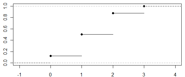
Figure 7.1. DF

In the next section, we are going to discover properties of the cdf in the discrete approach. Next, we will take these properties as the definition of a cdf of an arbitrary rrv. By this way, it will be easy to introduce continuous rrv.

The properties of cdf’s are given in the following proposition.

Proposition 2.

Let $F_{X}$ be the cdf of a discrete random variable $X$. Then, $F_{X}$ fulfills the following properties :

(1) $0\leq F_{X}\leq 1.$

(2) $\lim_{x\rightarrow-\infty}F_{X}(x)=0$ and $\lim_{x\rightarrow+\infty}F_{X}(x)=1$.

(3) $F_{X}$ is right-continuous.

(4) $F_{X}$ is $1$-non-decreasing, that is for $a\leq b$, $(a,b)\in\mathbb{R}^{2}$,

(7.0.3) $$\Delta_{a,b}F_{X}=F_{X}(b)-F_{X}(a)\geq 0.$$

Other terminology. We will also say that $F_{X}$ assigns non-negative lengths to intervals $[a,b]$, $a\leq b$. We will come back to this terminology.

Proof.

A general remark. In the proof below, we will have to deal with limits of $F_{X}$. But $F_{X}$ will be proved to be non-decreasing in Point (4). By Calculus Courses, general limits of non-decreasing functions, whenever they exist, are the same as monotone limits. So, when dealing with limits of $F_{X}$, we restrict ourselves to monotone limits.

In the sequel, a broadly increasing (resp. decreasing) sequence to something should be interpreted as a non strictly increasing (resp. decreasing) to something.

Consequently, we begin by the proof of Point (4).

Proof of (4). Let $a$ and $b$ be real numbers such that $a\leq b$, then $(X\leq a)\subset(X\leq b)$. Since probability measures are non-decreasing, we get

$$F_{X}(a)=\mathbb{P}(X\leq a)\leq\mathbb{P}(X\leq b)=F_{X}(b),$$

and then

$$\Delta_{a,b}F_{X}=F_{X}(b)-F_{X}(a)\geq 0,$$

which is the targeted Formula 7.0.3.

Proof of (1). The proof of (1) is immediate since for any $x\in\mathbb{R}$, $F_{X}(x)$ is probability value.

Proof of (2).

First, consider a sequence $t(n),n\geq 1$, that broadly decreases to $-\infty$ as $n\uparrow+\infty$, that is $t(n)\downarrow-\infty$. Let $A_{t(n)}=(X\leq t(n))$. Then, the sequence of events $(A_{t(n)})$ broadly decreases to $\emptyset$, that is

$$\bigcap_{n\geq 1}A_{t(n)}=\emptyset.$$

By the continuity of Probability measures (See Properties (D) and (E) in Chapter 2), we have

$$0=\mathbb{P}(\emptyset)=\lim_{n\uparrow+\infty}\mathbb{P}(A_{t(n)}),$$

that is, $F_{X}(t(n))\downarrow 0$ for any sequence $t(n)\downarrow-\infty$ as $n\uparrow+\infty$. By the previous remark on monotone limits, this means that

$$\lim_{x\rightarrow-\infty}F_{X}(x)=0.$$

Similarly, consider a broadly increasing sequence $t(n),n\geq 1$, to $+\infty$ as $n\uparrow+\infty$, that is $t(n)\uparrow+\infty$. Let $A_{t(n)}=(X\leq t(n))$. Then, the sequence of events $(A_{t(n)})$ broadly increases to $\Omega$, that is

$$\bigcup_{n\geq 1}A_{t(n)}=\Omega.$$

By the continuity of Probability measures (See Properties (D) and (E) in Chapter 2), we have

$$1=\mathbb{P}(\Omega)=\lim_{n\uparrow+\infty}\mathbb{P}(A_{t(n)}),$$

that is, $F_{X}(t(n))\uparrow 1$ for any sequence $t(n)\uparrow+\infty$ as $n\uparrow+\infty$. By the previous remark on monotone limits, this means that

$$\lim_{x\rightarrow+\infty}F_{X}(x)=1.$$

The proof of Point (2) is over.

Proof of 3. Let us show that $F_{X}$ is right-continuous at any point $x\in\mathbb{R}$. Let $h(n),n\geq 1$ a sequence of real and non-negative numbers decreasing to $0$ in a broad sense, that is $h(n)\downarrow 0$ as $n\uparrow+\infty$. We clearly have (use a drawing if not clear) that

$$\left(-\infty,x+h(n)\right]\downarrow\left(-\infty,x\right]\ \ as\ \ n\uparrow+\infty.$$

By using the fact that an inverse image mapping $X^{-1}$ preserves sets operations, we get that, as $n\uparrow+\infty$,

$$A_{x+h(n)}=(X\leq x+h(n))=X^{-1}(\left(-\infty,x+h(n)\right])\downarrow X^{-1}(\left(-\infty,x\right])=(X\leq x)=A_{x},$$

By the continuity of Probability measures (See Properties (D) and (E) in Chapter 2), we have

$$\mathbb{P}(A_{x+h(n)})\downarrow\mathbb{P}(A_{x}),$$

that is $F_{X}(x+h(n))\downarrow F_{X}(x)$, for any sequence $h(n)\downarrow 0$ as $n\uparrow+\infty$. From Calculus Courses, this means that

$$F_{X}(x+h)\downarrow F_{X}(x)\ \ as\ \ 0<h\rightarrow 0$$

Hence $F_{X}$ is right-continuous at $x$.

The previous properties allow us to state a general definition of the notion of cumulative distribution function and to unveil continuous real-valued random variables.

Let us begin by the general definition of a cumulative distribution function on $\mathbb{R}$.

Definition. A real-valued function $F$ defined on $\mathbb{R}$ is a cumulative distribution function if and only if

(1) $0\leq F\leq 1.$

(2) $\lim_{x\rightarrow-\infty}F(x)=0$ and $\lim_{x\rightarrow+\infty}F(x)=1$

(3) $F$ is right-continuous.

(4) $F$ is $1$-non-decreasing.

Random Variable associated with a cdf.

Before we begin, let us make some remarks on the domain of a probability measure. So far, we used discrete probability measures defined of the power set $\mathcal{P}(\Omega)$ of the sample set $\Omega$.

But it is possible to have a probability measure that is defined only on a subclass $\mathcal{A}$ of $\mathcal{P}(\Omega)$. In this case, we have to ensure the following points for the needs of the computations.

(1) The subclass $\mathcal{A}$ of $\mathcal{P}(\Omega)$ should contain the impossible event $\emptyset$ and the sure event $\Omega$.

(2) Since we use the sets operations (union, intersection, difference of sets, complements of sets, etc.), The subclass $\mathcal{A}$ of $\mathcal{P}(\Omega)$ should be stable under sets operations, but only when they are applied at most a countable number of times.

(3) For a real-valued random variable $X$, we need to define its cdf $F_{X}(x)$, $x\in\mathbb{R}$, we have to ensure that the events $(X\leq x)$ lie in $\mathcal{A}$ for all $x\in\mathbb{R}$.

The first two points hold for discrete probability measures when $\mathcal{A}=\mathcal{P}(\Omega)$ and the third point holds for a discrete real-valued random variable when $\mathcal{A}=\mathcal{P}(\Omega)$.

In general, a subclass $\mathcal{A}$ of $\mathcal{P}(\Omega)$ fulfilling the first two points is called a fields of subsets or a $\sigma$-algebra of subsets of $\Omega$. A real-value application $X$ defined on $\Omega$ such that events $(X\leq x)$ lie in $\mathcal{A}$ for all $x\in\mathbb{R}$, is called a measurable application, or a random variable, with respect to $\mathcal{A}$.

The consequence is that, you may see the symbol $\mathcal{A}$ and read about measurable application in the rest of this chapter and subsequent chapters. But, we do not pay attention to them. We only focus on the probability computations, assuming everything is well defined and works well, at least at this level. We will have time and space for such things in the mathematical course on Probability Theory .

Now, it is time to introduce our definitions.

Definition. Given a cdf $F$, we say that a random variable $X$ defined on some probability space $(\Omega,\mathcal{A},\mathbb{P})$ possesses (or, is associated to) the cdf $F$, if and only if

(7.0.4) $$\mathbb{P}(X\leq x)=F(x),\ \ for\ all\ \ x\in\mathbb{R},$$

that is $F_{X}=F$. Each particular cdf is associated to a name of probability law that applies both to the cdf and to the rrv.

Immediate examples

Let us give the following examples.

Exponential law with parameter $\lambda>0$, denoted $\mathcal{E}(\lambda)$.

A rrv $X$ follows an Exponential law with parameter $\lambda>0$, denoted $X\sim\mathcal{E}(\lambda)$ if and only if its cdf is given by

$$F(x)=\left\{\begin{array}[]{c}1-e^{-\lambda x}\text{ \ \ \ }x\geq 0\\ 0\text{ \ \ \ \ \ \ \ \ \ \ \ \ \ }x<0.\end{array}\right.$$

Uniform law on $(a,b)$, denoted $\mathcal{U}(a,b)$, $a<b$.

A rrv $X$ follows a uniform law on $[a,b]$, $a<b$, denoted $X\sim\mathcal{U}(a,b)$, if and only if its cdf is given by

$F(x)=\left\{\begin{tabular}[]{lll}$1$&$if$&$x>b$\\ $(x-a)/(b-a)$&$if$&$a\leq x\leq b$\\ $0$&$if$&$x<a.$\end{tabular}.\right.$

These two functions are clearly cdf’s. Besides, they are continuous cdf’s.

Let us begin by definitions and examples.

Let $F_{X}$ be the cdf of a rrv $X$. Suppose that $F_{X}$ satisfies :

(a)

$$\text{ \ \ \ \ }f_{X}=F_{X}^{\prime}=\frac{dF_{X}}{dx}\text{ exists on }\mathbb{R}$$

and

(b)

$$f_{X}=F_{X}^{\prime}\text{ is integrable on intervals }[s,t],\ s<t.$$

Then for any $b<x\in\mathbb{R}$

$$F_{X}(x)-F_{X}(b)=\int_{b}^{x}F_{X}^{\prime}(t)dt,\ \ x\in\mathbb{R}.$$

When $b\downarrow-\infty$, we get for $x\in\mathbb{R}$,

(7.0.5) $$F_{X}(x)=\int_{-\infty}^{x}f_{X}(t)\text{ }dt.$$

We remark that $f_{X}$ is non-negative as the derivative of a non-decreasing function. Next, by applying Formula (7.0.5) to $+\infty$, we get that

$$1=\int_{-\infty}^{+\infty}f_{X}(t)dt.$$

In summary, under our assumptions, there exists a function $f_{X}$ satisfying

(7.0.6) $$f_{X}(x)\geq 0,\text{for all }x\in\mathbb{R},$$

and

(7.0.7) $$\int_{-\infty}^{+\infty}f_{X}(t)dt=1.$$

We say that $X$ is an absolutely continuous random variable and that $f_{X}$ is its probability density function (pdf). This leads us to the following definition.

Definition. A function $f:\mathbb{R}\rightarrow\mathbb{R}$ is a probability density function (pdf) if and only if Formulas (7.0.6) and (7.0.7) hold.

Definition. A rrv is said to have an absolutely continuous probability law if and only if there exists a pdf denoted by $f_{X}$ such that (7.0.5) holds.

The name absolutely continuity is applied to the probability law and to the random variable itself and to the cdf.

Definition: The domain or the support of an absolutely continuous random variable is defined by

(7.0.8) $$\mathcal{V}_{X}=\{x\in\mathbb{R},f_{X}(x)\neq 0\}.$$

Remark for advanced readers. Actually, we need to take the closure of that set. But, at this earlier stage, we simplify things and fortunately, such simplifications do not impact the type of problems we treat here.

We saw that knowing the values set of a discrete rvv is very important for the computations. So is it for absolutely continuous rvv.

Examples. Let us return to the examples of the Exponential law and the uniform law. By deriving the cdf, we see that :

An exponential rvv with parameter $\lambda>0$, $X\sim\mathcal{E}(\lambda)$, is absolutely continuous with pdf

$$f(x)=\lambda exp(-\lambda x)1_{(x\geq 0)},$$

with support

$$\mathcal{V}_{X}=\mathbb{R}_{+}=\{x\in\mathbb{R},\ x\geq 0\}.$$

A uniform (or uniformly distributed) random variable on $[a,b]$, $a<b$, $X\sim\mathcal{U}(a,b)$, is absolutely continuous with pdf

$$f(x)=\frac{1}{b-a}1_{(a\leq x\leq b)},$$

and with domain

$$\mathcal{V}_{X}=[a,b].$$

In this subsection, we are going to present two important classes of distribution functions : the Gamma and the Gaussian classes. But we begin by showing a general way of finding pdf’s.

I - A general way of finding pdf’s.

A general method of finding a pdf is to consider a non-negative function $g\geq 0$ which is integrable on $\mathbb{R}$ such that the integral on $\mathbb{R}$ is strictly positive, that is

$$C=\int_{\mathbb{R}}g(x)dx>0.$$

We get a pdf $f\geq 0$ of the form

$$f(x)=C^{-1}\ g(x),\ x\in\mathbb{R}.$$

Here are some examples.

II - Gamma Law $\gamma(a,b)$ with parameters $a>0$ and $b>0$.

(a) Definition. Let

$$\Gamma(a)=\int_{0}^{+\infty}x^{a-1}e^{-x}dx.$$

The function

$$f_{\gamma(a,b)}(x)=\frac{b^{a}}{\Gamma(a)}x^{a-1}e^{-bx}1_{(x\geq 0)}$$

is a pdf. A non-negative random variable $X$ admitting $f_{\gamma(a,b)}$ as a pdf is said to follow a Gamma law $\gamma(a,b)$ with parameter $a>0$ and $b>0,$ denoted as $X\sim\gamma(a,b)$.

Important remark. An exponential $\mathcal{E}(\lambda)$ random variable, with $\lambda>0$ is also a $\gamma(1,\lambda)$ rrv.

We have in Figure 7.2 graphical representations of probability density functions depending of the parameter $\lambda$. In Figure 7.3, probability density functions of $\gamma$ laws are illustrated.

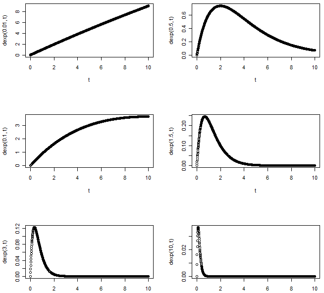
Figure 7.2. Exponential Probability Density Function s

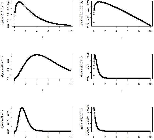
Figure 7.3. $\gamma$-Probability Density Function s

Justification. From Calculus courses, we may justify that the following function

$$x^{a-1}e^{-bx}1_{(x>0)}$$

is integrable on its domain $\mathbb{R}_{+}$ and we denote

(7.0.9) $$\Gamma(a,b)=\int_{0}^{+\infty}x^{a-1}e^{-bx}dx>0.$$

We obtain a pdf

$$\frac{1}{\Gamma(a,b)}x^{a-1}e^{-bx}1_{(x>0)}.$$

If $b=1$ in (7.0.9), we denote

$$\Gamma(a)=\Gamma(a,1)=\int_{0}^{+\infty}x^{a-1}e^{-x}dx.$$

The function $\Gamma(\circ)$ satisfies the relation

(7.0.10) $$\forall(a>1),\text{ \ }\Gamma(a)=(a-1)\Gamma(a-1).$$

This comes from the following partial integration

$$\Gamma(a) = \int_{0}^{+\infty}x^{a-1}d(-e^{-x})$$

$$= \left[-x^{a-1}e^{-x}\right]_{0}^{+\infty}+(a-1)\int_{0}^{+\infty}x^{a-2}e^{-x}dx$$

$$= 0+(a-1)\Gamma(a-1).$$

We also remark that

(7.0.11) $$\Gamma(1)=1,$$

since

$$\Gamma(1)=\int_{0}^{+\infty}e^{-x}dx=\int_{0}^{+\infty}d(-e^{-x})=\left[-e^{-x}\right]_{0}^{+\infty}=1.$$

So, by applying (7.0.10) to integers $a=n\in\mathbb{N}$, $n\geq 1$, and by taking (7.0.11) into account, we get by induction that

$$\forall(n\in\mathbb{N}\setminus\{0\}),\text{ }\Gamma(n)=(n-1)!.$$

Finally, we have

(7.0.12) $$\forall(a>0,b>0),\text{ }\Gamma(a,b)=\frac{\Gamma(a)}{b^{a}}.$$

This comes from the change of variables $u=bx$ in (7.0.9) which gives

$$\Gamma(a,b) = \int_{0}^{+\infty}\left(\frac{u}{b}\right)^{a-1}e^{-u}\left(\frac{du}{b}\right)$$

$$= \frac{1}{b^{a}}\int_{0}^{+\infty}u^{a-1}e^{-u}du$$

$$= \frac{\Gamma(a)}{b^{a}}.$$

The proof is concluded by putting together (7.0.9), and (7.0.10), and (7.0.11), and (7.0.12).

III - Gaussian law $\mathcal{N}(m,\sigma^{2})$ with parameters $m\in\mathbb{R}$ and $\sigma^{2}>0$ .

(a) Definition. A random variable $X$ admitting the pdf

(7.0.13) $$f(x)=\frac{1}{\sigma\sqrt{2\pi}}\exp\left(-\frac{(x-m)^{2}}{2\sigma^{2}}\right),\ \ x\in\mathbb{R},$$

is said to follow a normal or a Gaussian law of parameters $m\in\mathbb{R}$ and $\sigma^{2}>0,$ denoted by

$$X\sim\mathcal{N}(m,\sigma^{2})$$

The probability density function of the standard Gaussian Normal variable is illustrated in Figure 7.4.

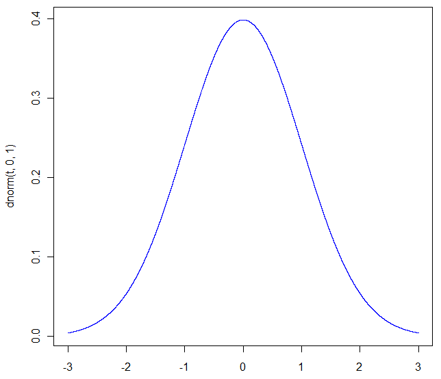
Figure 7.4. Probability Density Function of a Standard Gaussian Random Variable

(b) Justification. The justification comes from the computation

of

$$I=\int_{-\infty}^{+\infty}\exp\left(-\frac{(x-m)^{2}}{2\sigma^{2}}\right)dx.$$

By the change of variable

$$u=\frac{x-m}{\sigma\sqrt{2}},$$

we get

$$I=\sigma\sqrt{2}\int_{-\infty}^{+\infty}e^{-u^{2}}du.$$

Advanced readers already know the value of $I$. Other readers, especially those in the first year of University, have to know that a forwarding Calculus course on multiple integration will show

$$\int_{-\infty}^{+\infty}e^{-u^{2}}du=\sqrt{\pi},$$

so that we arrive at

$$I=\sigma\sqrt{2\pi}.$$

This justifies that

$$\frac{1}{\sigma\sqrt{2\pi}}\exp\left(-\frac{(x-m)^{2}}{2\sigma^{2}}\right),x\in\mathbb{R},$$

is a pdf.

But in this chapter, we will provide elementary methods based on the earlier works of de Moivre (1732) and Laplace (1801) to directly proof that

$$J=\int_{-\infty}^{+\infty}\frac{1}{\sqrt{2\pi}}\exp\left(-t^{2}/2\right)\ dt=1,$$

which proves that (7.0.13) is a pdf for $m=0$ and $\sigma=1$. For proving the general case of arbitrary $m$ and $\sigma^{2}>0$, we can use the change of variable $u=(x-m)/\sigma$ to see that $I=\sigma\sqrt{1\pi}$.

Commentary. This Gaussian law is one of the most important probability laws both in Probability Theory and in Statistics. It will be a key tool in the next courses on Probability Theory and Mathematical Statistics.

By now, we want to devoted a full section on some historical facts and exhibit the first central limit theorem through the de Moivre and Laplace theorems.

Warning. The reader is not obliged to read this section. The results of this section are available in modern books with elegant proofs. But, those who want acquire a deep expertise in this field are invited to read such a section because of its historical aspects. They are invited to discover the great works of former mathematicians.

A very important example of absolutely continuous cdf is the Gaussian rrv. There are many ways to present it. Here, in this first course, we want to show the reader the very historical way to derive it from the Binomial law, through the de Moivre and Laplace theorems (1732 - 1801).

Here, the standard Gaussian law with $m=0$ and $\sigma=1$ is derived as an approximation of centered and normalized Binomial random variable s.

Let $(X_{n})_{n\geq 1}$ be a sequence of Bernoulli random variables of respective parameters $n$ and $p$,    that is, for each $n\geq 1$, $X_{n}\sim\mathcal{B}(n,p)$. We recall the following parameters of such rrv’s :

$$\mathbb{E}(X_{n})=np\text{ and }Var(X_{n})=npq.$$

Put

$$Z_{n}=\frac{X_{n}\text{ }-\text{ }np}{\sqrt{npq}}.$$

We have $\mathbb{E}(Z_{n})=0$ and $Var(Z_{n})=1$. Here are historical results.

Theorem 4.

(de Moivre, 1732, see loeve , page 23) .

The equivalence

$$\mathbb{P}(X_{n}=j)\sim\frac{e^{-\frac{x^{2}}{2}}}{\sqrt{2^{\pi}npq}},$$

holds uniformly in

$$x=\frac{(j\text{ }-\text{ }np)}{\sqrt{2^{\pi}npq}}\in\left[a,\text{ }b\right],a<b.$$

as $n\rightarrow\infty.$

Next, we have:

Theorem 5.

(Laplace 1801, see loeve , page 23) .

(1) For any $b<a$, we have

$$\mathbb{P}(b\leq Z_{n}\leq a)\rightarrow\int_{b}^{a}\frac{1}{\sqrt{2\pi}}\text{ }e^{-\frac{x^{2}}{2}}dx.$$

(2) For any $x\in\mathbb{R}$, we have

$$\mathbb{P}(Z_{n}\leq x)\rightarrow\int_{-\infty}^{x}\frac{1}{\sqrt{2\pi}}\text{ }e^{-\frac{x^{2}}{2}}dx.$$

(3) The function

$$\frac{1}{\sqrt{2\pi}}\text{ }e^{-\frac{x^{2}}{2}}dx,\ x\in\mathbb{R},$$

is a probability distribution function.

Proofs of the results.

(A) Proof of Theorem 4.

At the beginning, let us recall some needed tools.

(i) $f_{n}(x)\rightarrow f(x)$ uniformly in $x\in A$, as $n\rightarrow\infty$, means that

$$\lim_{n\rightarrow\infty}\sup_{x\in A}\text{ }\left|f_{n}(x)-f(x)\right|=0.$$

(ii) $f_{n}(x)\sim f(x)$, as $n\rightarrow\infty$, for a fixed $x,$ mean s

$$\lim_{n\rightarrow\infty}\text{ }\frac{f_{n}(x)}{f(x)}=1.$$

(iii) $f_{n}(x)\sim f(x)$ uniformly in $x\in A$, as $n\rightarrow\infty$, means that

$$\lim_{n\rightarrow\infty}\sup_{x\in A}\text{ }\left|\left(\frac{f_{n}(x)}{f(x)}\right)-1\right|=0.$$

(iv) $a_{n}=0(b_{n})$ as $n\rightarrow\infty$, mean s that

$$\exists\text{ \ }M\text{ }>\text{ }0,\text{ }\exists\text{ \ }N,\text{ \ }\forall\text{ }n\geq N,\text{ }\left|\frac{a_{n}}{b_{n}}\right|\text{ }<\text{ }M.$$

(v) $a_{n}(x)=0(b_{n}(x))$ uniformly in $x\in A,$ as $n\rightarrow\infty,$ means that

$$\exists\text{ \ }M\text{ }>\text{ }0,\text{ }\exists\text{ \ }N,\text{ }\forall\text{ }n\geq N,\text{ }\forall\text{ }x\in A,\text{ }\left|\frac{a_{n}(x)}{b_{n}(x)}\right|\text{ }<\text{ }M.$$

(vi) We will need the Sterling Formula we studied in Chapter 1:

$$n!=\sqrt{2\pi n}\text{ }n^{n}\text{ }e^{-n}\text{ }e^{\theta_{n}},$$

where for any $\eta>0$, we have for $n$ large enough,

$$\left|\theta_{n}\right|\leq\frac{1+\eta}{(12n)}.$$

We begin the proof by denoting $k=n-j,$ $q=1-p,$ and by writing

(7.0.14) $$S_{n}(j)=\mathbb{P}(X_{n}=j)=\left(\frac{1}{\sqrt{2\pi}}\right)\sqrt{(\frac{n}{jk})}\left(\frac{np}{j}\right)^{j}\text{ }\left(\frac{nq}{k}\right)^{k}\text{ }e^{\theta_{n}}e^{-\theta_{j}}e^{-\theta_{k}}.$$

Hence

(7.0.15) $$x=\frac{(j-np)}{\sqrt{2\pi npq}}\in\left[a,\text{ }b\right]\Leftrightarrow np-a\sqrt{npq}\leq j\leq np-b\sqrt{npq}$$

(7.0.16) $$\Leftrightarrow nq-b\sqrt{npq}\leq k\leq nq-a\sqrt{npq}.$$

Hence $j$ and $k$ tend to $+\infty$ uniformly in $x=\frac{(j-np)}{\sqrt{2\pi npq}}\in\left[a,\text{ }b\right].$ Then $e^{-\theta_{j}}\sim 1$ and $e^{-\theta_{k}}\sim 1$, uniformly in $x=\frac{(j-np)}{\sqrt{2\pi npq}}\in\left[a,\text{ }b\right]$ as $n\rightarrow\infty.$ Let us use the following second order expansion of $\log(1+u):$

(7.0.17) $$\log(1+u)=u-\frac{1}{2}u^{2}+O(u^{3}),\text{ as }u\rightarrow 0.$$

Then, there exist a constant $C>0$ and a number $u_{0}$ $>$ $0$ such that

$$\forall(0\leq u\leq u_{0}),\text{ }\left|O(u^{3})\right|\leq C\ u^{3}.$$

We have,

$$\frac{j}{(np)}=\left(1+x\sqrt{\frac{q}{(np)}}\right)$$

$$\left|x\sqrt{\frac{q}{(np)}}\right|\leq\max(\left|a\right|,\left|b\right|)\sqrt{\frac{q}{(np)}}\rightarrow 0,$$

uniformly in $\ x\in\left[a,\text{ }b\right].$ Combining this with (7.0.17) leads to

$$\left(\frac{np}{j}\right)^{j}=\exp\left(-\text{ }j\text{ }\log(\frac{j}{np})\right).\text{ \ \ \ }$$

But we also have

$$\log\left(\frac{j}{np}\right)=\log\left(1+x\sqrt{\frac{q}{(np)}}\right)$$

(7.0.18) $$=x\sqrt{\frac{q}{(np)}}-x^{2}\text{ }\frac{q}{\left[2(np)\right]}+O(n^{-\frac{1}{2}}).$$

We remark that the big $O,$ which does not depend on $n$ nor on $x,$ is uniformly bounded. By using $j=np+x\sqrt{\frac{q}{(np)}}$ in (7.0.18), and by operating the product, we get

$$j\text{ }\log\left(\frac{j}{np}\right)=x\sqrt{npq}+x^{2}\frac{q}{2}+0(n^{-\frac{1}{2}})$$

and then,

(7.0.19) $$\left(\frac{np}{j}\right)^{j}=\exp\left(\text{ }-\text{ }\sqrt{npq}-x^{2}\frac{q}{2}+0(n^{-\frac{1}{2}})\right).$$

We just proved that

(7.0.20) $$\left(\frac{np}{k}\right)^{j}=\exp\left(\text{ }+\sqrt{npq}-x^{2}\frac{p}{2}+0(n^{-\frac{1}{2}})\right).$$

The product gives

(7.0.21) $$\left(\frac{np}{j}\right)^{j}\left(\frac{np}{k}\right)^{j}=\exp\left(\text{ }-\frac{1}{2}x^{2}\right)\exp\left(\text{ }0(n^{-\frac{1}{2}})\right),$$

where the big $0(n^{-\frac{1}{2}})$ uniformly holds in

$$x=\frac{(j\text{ }-\text{ }np)}{\sqrt{2^{\pi}npq}}\in\left[a,\text{ }b\right],a<b.$$

The proof is finished by combining (7.0.21) and consequences of (7.0.15) and (7.0.16).

Proof of Theorem 5.

Let $j_{0}=np+a\sqrt{npq}.$ Let $j_{h},$ $h=1,...,m_{n-1},$ be the intergers between $j_{0}$ and $np+b\sqrt{npq}=j_{m_{n}}$ and denote

$$x_{h}=\frac{(j_{h}-np)}{\sqrt{npq}}.$$

It is immediate that

(7.0.22) $$\max_{0\leq h\leq m_{n-1}}\text{ }j_{h+1}-j_{h}\leq\frac{1}{\sqrt{npq}}.\text{ }$$

By the Laplace-Moivre-Gauss Theorem 4, we have

(7.0.23) $$\mathbb{P}(X_{n}=j_{h})=\frac{e\frac{-x_{h}^{z}}{2}}{\sqrt{2\pi npq}}(1+\varepsilon_{n}(h)),\text{ }h=1,......,m_{n-1}$$

with

(7.0.24) $$\underset{1\leq h\leq m_{n-1}}{\max}\left|\varepsilon_{n}(h)\right|=\varepsilon\rightarrow 0$$

as $n\rightarrow+\infty.$ But,

$$\mathbb{P}(a<Z_{n}<b)=\sum_{1\leq h\leq m_{n-1}}\mathbb{P}(X_{n}=j_{h}).\$$

(7.0.25) $$=\sum_{1\leq h\leq m_{n-1}}\frac{e\frac{-x_{h}^{z}}{2}}{\sqrt{2\pi npq}}+\sum_{1\leq h\leq m_{n-1}}\frac{e\frac{-x_{h}^{z}}{2}}{\sqrt{2\pi npq}}\text{ }\varepsilon_{n}(h).$$

$$=\sum_{1\leq h\leq m_{n-1}}\frac{e\frac{-x_{h}^{z}}{2}}{\sqrt{2\pi npq}}(1+\varepsilon_{n}(h))$$

Also, we have

$$\underset{n\rightarrow\infty}{\lim}\ \sum_{1\leq h\leq m_{n-1}}\frac{e\frac{-x_{h}^{z}}{2}}{\sqrt{2\pi npq}}=\sum_{0\leq h\leq m_{n}}\frac{e\frac{-x_{h}^{z}}{2}}{\sqrt{2\pi npq}}$$

since each of the two terms that were added converges to 0. The latter expression is a Riemann sum on $\left[a,\text{ }b\right]$ based on a uniform subdivision and associated to the function $x\mapsto e^{-\frac{x^{2}}{2}}.$ This function is continuous on $[a,b],$ and therefore, is integrable on $[a,b].$ Therefore the Riemann sums converge to the integral

$$\frac{1}{\sqrt{2\pi}}\int_{a}^{b}e^{-\frac{x^{2}}{2}}dx.$$

This means that the first term of (7.0.25) satisfies

(7.0.26) $$\sum_{1\leq h\leq m_{n-1}}\frac{e\frac{-x_{h}^{z}}{2}}{\sqrt{2^{\pi}npq}}\rightarrow\left(\frac{1}{\sqrt{2^{\pi}}}\right)\int_{a}^{b}e^{-\frac{x^{2}}{2}}dx.$$

The second term (7.0.25) satisfies

(7.0.27) $$0\leq\sum_{1\leq h\leq m_{n-1}}\frac{e^{-\frac{x_{h}^{2}}{2}}}{\sqrt{2^{\pi}npq}}\varepsilon_{n}(h)\leq\varepsilon_{n}\sum_{1\leq h\leq m_{n-1}}\frac{e^{-\frac{x_{h}^{2}}{2}}}{\sqrt{2^{\pi}npq}}.$$

Because, the sequence

$$\varepsilon_{n}=\sup\{\left|\varepsilon_{n}(h)\right|,0\leq h\leq m_{n}\}$$

goes to zero based on (7.0.24) above, and of (7.0.26), it comes that second term of (7.0.25) tends to zero. This establishes Point (1) of the theorem. Each of the signs $<$ and $>$ may be replaced $\leq$ or $\geq.$ The effect in the proof would result in adding of at most two indices  in the sequence $i_{1},...,i_{m_{n}-1}$ ( $j_{0}$ and/or $j_{m_{n}})$ and the corresponding terms of this or these two indices in (7.0.25) tend to zero and the result remains valid.

Let us move to the two other points. We have

$$\underset{t\rightarrow\infty}{\lim}t^{2}e^{-\frac{t^{2}}{2}}=0.$$

Thus, there exists $A>0$ such that

(7.0.28) $$\left|t\right|\geq A\Rightarrow 0\leq e^{-\frac{t^{2}}{2}}<\frac{1}{t^{2}}.$$

Then, for $a>A$ and $b<-A$

$$\int_{b}^{a}e^{-\frac{t^{2}}{2}}dt\leq\int_{-A}^{A}e^{-\frac{t^{2}}{2}}dt+\int_{b}^{-A}e^{-\frac{t^{2}}{2}}dt+\int_{A}^{a}e^{-\frac{t^{2}}{2}}dt$$

$$\leq \int_{-A}^{A}e^{-\frac{t^{2}}{2}}dt\ +\int_{-\infty}^{-A}e^{-\frac{t^{2}}{2}}dt+\int_{A}^{+\infty}e^{-\frac{t^{2}}{2}}dt$$

$$\leq \int_{-A}^{A}e^{-\frac{t^{2}}{2}}dt\ +2\int_{A}^{+\infty}e^{-\frac{t^{2}}{2}}dt$$

$$\leq \int_{-A}^{A}e^{-\frac{t^{2}}{2}}dt\ +2\int_{A}^{+\infty}\frac{1}{t^{2}}dt\text{ \ \ (By \ref{gauss001})}$$

$$= \int_{-A}^{A}e^{-\frac{t^{2}}{2}}dt\ +\frac{2}{A}.$$

The inequality

(7.0.29) $$\int_{b}^{a}e^{-\frac{t^{2}}{2}}dt\leq\int_{-A}^{A}e^{-\frac{t^{2}}{2}}dt\ +\frac{2}{A},$$

remains true if $a\leq A$ or $b\geq-A$. Thus, Formula (7.0.29) holds for any real numbers $a$ and $b$ with $a<b$. Since

$$\int_{b}^{a}e^{-\frac{t^{2}}{2}}dt$$

is increasing as $a\uparrow\infty$ and $b\downarrow-\infty,$ it comes from Calculus courses on limits that its limit as $a\rightarrow\infty$ and $b\rightarrow-\infty$, exists if and only if it is bounded. This is the case with 7.0.29. Then

$$\lim_{a\rightarrow\infty,b\rightarrow-\infty}\int_{b}^{a}e^{-\frac{t^{2}}{2}}dt=\int_{-\infty}^{\infty}e^{-\frac{t^{2}}{2}}dt\in\mathbb{R}\$$

We denote

$$G(x)=\int_{-\infty}^{x}e^{-\frac{t^{2}}{2}}dt\in\mathbb{R}$$

and

$$F_{n}(x)=\mathbb{P}(Z_{n}\leq x),x\in\mathbb{R}.$$

It is clear that $G(x)\rightarrow 0$ as $x\rightarrow-\infty$.  Thus, for any $\varepsilon>0$, there exists $b_{1}<0$ such that

$$\forall\text{ }b\leq b_{1},\text{ }G(b)\leq\frac{\varepsilon}{3}$$

For any $b<0$, we apply the Markov’s inequality, to have

$$\mathbb{P}(Z_{n}\leq b)\leq\mathbb{P}\left(\left|Z_{n}\right|\geq\left|b\right|\right)\leq\frac{\mathbb{E}\left|Z_{n}\right|^{2}}{\left|b\right|^{2}}=\frac{1}{\left|b\right|^{2}},$$

by the fact that $\mathbb{E}Z_{n}=0,$

$$\mathbb{E}\left|Z_{n}\right|^{2}=\mathbb{E}Z_{n}^{2}=var(Z_{n})=1.$$

Then, for any $\varepsilon>0$, there exist $b_{2}<b_{1}$ such that

$$\forall\text{ }b\leq b_{2},\text{ }F_{n}(b)=\mathbb{P}(Z_{n}\leq b)\leq\frac{\varepsilon}{3}$$

By $Point$ (1), for any $a\in\mathbb{R},$ and for $b\leq\min(b_{2},a),$ there exists $n_{0}$ such that for $n\geq n_{0},$

$$\left|(F_{n}(a)-F_{n}(b))-(G(a)-G(b))\right|\leq\frac{\varepsilon}{3}\text{.}$$

We combine the previous facts to get that for any $\varepsilon>0,$ for any $a\in\mathbb{R}$, there exists $n_{0}$ such that for $n\geq n_{0},$

$$\left|F_{n}(a)-G(a)\right| \leq \left|(F_{n}(a)-F_{n}(b_{0}))-(G(a)-G(b_{0}))\right|+\left|F_{n}(b_{0})-G(b_{0})\right|$$

$$\leq \frac{\varepsilon}{3}+\left|F_{n}(b_{0})\right|+\left|G(b_{0})\right|\leq\frac{\varepsilon}{3}+\frac{\varepsilon}{3}+\frac{\varepsilon}{3}=\varepsilon\text{.}$$

We conclude that for any $a\in\mathbb{R},$

$$\mathbb{P}(Z_{n}\leq a)\rightarrow G(a)=\frac{1}{\sqrt{2^{\pi}}}\int_{-\infty}^{a}e^{-\frac{t^{2}}{2}}dt\text{. }$$

This gives Point (2) of the theorem.

The last thing to do to close the proof is to show Point (3) by establishing that $G(\infty)=1$. By the Markov’s inequality and the remarks done above, we have for any $a>0$,

$$\mathbb{P}(Z_{n}>a)\leq\mathbb{P}(\left|Z_{n}\right|>a)<\frac{1}{a^{2}}$$

Then for any $\varepsilon>0,$ there exists $a_{0}>0$ such that

$$\mathbb{P}(Z_{n}>a)<\varepsilon\text{.}$$

This is equivalent to saying that there exists $a_{0}>0$ such that for any $a\geq a_{0}$ and for any $n\geq 1,$

$$1-\varepsilon\leq F_{n}(a)\leq 1\text{. }$$

By letting $n\rightarrow\infty$ and by using Point (2), we get for any $a\geq a_{0},$

$$1-\varepsilon\leq G(a)\leq 1\text{.}$$

By the monotonicity of $G,$ we have that $G(\infty)$ is the limit of $G(a)$ as $a\rightarrow\infty$. So, by letting $a\rightarrow\infty$ first and next $\varepsilon\downarrow 0$ in the last formula, we arrive at

$$1=G(+\infty)=\frac{1}{\sqrt{2^{\pi}}}\int_{-\infty}^{+\infty}e^{-\frac{t^{2}}{2}}dt.$$

This is Point (3).

We need to make computations in solving problems based on probability theory. Especially, when we use the cumulative distribution functions $F_{X}$ of some real-valued random variable, we need some times to find the numerical value of $F(x)$ for a specific value of $x$. Sometimes, we need to know the quantile function (to be defined in the next lines). Some decades ago, we were using probability tables, that you can find in earlier versions of many books on probability theory, even in some modern books.

Fortunately, we now have free and powerful software packages for probability and statistics computations. One of them is the software R. You may find at www.r-project.org the latest version of R. Such a software offer almost everything we need here.

Let us begin by the following problem.

Example. The final exam for a course, say of Geography, is composed by $n=20$ Multiple Choice Questions (MCQ). For each equation, $k$ answers are proposed and only one them is true. The students are asked to answer each question by choosing one the $k$ proposed answers. At the end of the test, the grade of each student is the total number of correct answers. A student passes the exam if and only if he has at least the grade $x=10$ over $n$.

One of the students, say Jean, decides to answer at random. Let $X$ be his possible grade before the exam. Here $X$ follows a binomial law with parameters $n=20$ and $p=1/4$. So the probability he passes is

$$p_{pass}=\mathbb{P}(X\geq x)=\sum_{x\leq j\leq n}=\mathbb{P}(X=j).$$

We will give the solution as applications of the material we are going to present. We begin by introducing the quantile function.

A - Quantile function.

Let $F:\mathbb{R}\rightarrow[0,1]$ be a cumulative distribution function. Since $F$ is already non-decreasing, it is invertible if it is continuous and increasing. In that case, we may use the inverse function $F^{-1}$, defined by

$$\forall s\in[0,1],\ \forall x\in\mathbb{R},\ F(x)=s\Leftrightarrow x=F^{-1}(s).$$

In the general case, we may also define the generalized inverse

$$\forall s\in[0,1],\ F^{-1}(s)=\inf\{x\in\mathbb{R},\ F(x)\geq s\}.$$

we have the following interesting properties

$$\forall s\in[0,1],\forall x\in\mathbb{R},\ (F^{-1}(s)\leq x)\Leftrightarrow(s\leq F(x))$$

$$\forall s\in[0,1],\forall x\in\mathbb{R},\ (F^{-1}(s)>x)\Leftrightarrow(s>F(x))$$

$$\forall s\in[0,1],\ F(F^{-1}(s)-0)\leq s\leq F(F^{-1}(s)),$$

where

$$F(F^{-1}(s)+0)=\lim_{h\downarrow 0}F(F^{-1}(s)-h).$$

The generalized inverse is called the quantile function of $F$. Remember that the quantile function is the inverse function of $F$ if $F$ is invertible.

B - Installation of R.

Once you have installed R on your computer, and you launch, you will see the window given in Figure 7. You will write your command and press the ENTER button of your keyboard. The result of the graph is displayed automatically.

C - Numerical probabilities in R .

In R, each probability law has its name. Here are the most common ones in Table 7.1.

Distribution	R name	additional arguments
beta	beta	shape1, shape2, ncp
binomial	binom	size, prob
Cauchy	cauchy	location, scale
chi-squared	chisq	df, ncp
exponential	exp	rate
F	f	df1, df2, ncp
gamma	gamma	shape, scale
geometric	geom	prob
hypergeometric	hyper	m, n, k
log-normal	lnorm	meanlog, sdlog
logistic	logis	location, scale
negative binomial	nbinom	size, prob
normal	norm	mean, sd
Poisson	pois	lambda
Student’s t	t	df, ncp
uniform	unif	min, max
Weibull	weibull	shape, scale
Wilcoxon	wilcox	m, n

Table 7.1. Names of Probability laws in R

How to use each probability law ?

In column 2, under R name of Table 7.1, are listed the names of some random variables as they re used the Software R. In the last column, the names ate parameters are given.

Those names are used as follows :

(a) Add the letter p before the name to have the cumulative distribution function, that is called as follows:

$$pname(x,param1,param2,param3).$$

(b) Add the letter d before the name to have the probability density function (discrete or absolutely continuous), that is called as follows :

$$dname(x,param1,param2,param3).$$

(c) Add the letter q before the name to have the quantile function, that is called as follows

$$qname(x,param1,param2,param3).$$

Example. Let us use the Normal Random variable of parameters : mean ($m=0$) and variance ($sd=1$).

For $X\sim\mathcal{N}(0,1)$, we computed

$$p=\mathbb{P}(X\leq 1.96)$$

We may read in Figure 7 the value : $p=0.975$.

We may do more and get more values in Table 7.

Probability	argument	R command	values
$\mathbb{P}(X\leq-2)$	-2	pnorm(-2,0,1)	0.02275013
$\mathbb{P}(X\leq-1.95)$	-1.96	pnorm(-1.96,0,1)	0.02499790
$\mathbb{P}(X\leq-0.8)$	-0.8	pnorm(-0.8,0,1)	0.02275013
$\mathbb{P}(X\leq 0)$	0	pnorm(0,0,1)	0.5
$\mathbb{P}(X\leq 0.8)$	0.8	pnorm(0.2,0,1)	0.02275013
$\mathbb{P}(X\leq-1.96)$	1.96	pnorm(1.96,0,1)	0.975
$\mathbb{P}(X\leq 2)$	2	pnorm(2,0,1)	0.02275013

Exercise. Use the quantile function applied to the probabilities above to find the arguments. For example, set $u=0.02275013$, and use the R command

$$qnorm(u,0,1)$$

to find again $x=-2$.

Follow that example to learn how to use all the probability law. Now, we return back to our binomial example (page : 5).

D - Solution of the Lazy student problem using R.

We already know that the probability that he passes by answering at random is

$$p_{pass}=\mathbb{P}(X\geq x)=\sum_{x\leq j\leq n}=\mathbb{P}(X=j).$$

The particular values are : $n=20$, $p=0.25$, $x=10$. From Table 7.1, we see that the R name for the binomial probability is binom and its parameters are $n=size$ and $prob=p$. By using R, this probability is

$$p_{pass} = \mathbb{P}(X\geq 10)$$

$$= 1-\mathbb{P}(X\leq 10)$$

$$= 1-pbinom(9,20,0.25)=0.01386442.$$

So, he has only 13 chances over one thousand to pass.

Chapter 8 Appendix : Elements of Calculus

Calculus is fundamental to Probability Theory and Statistics. Especially, the notions on limits in $\mathbb{R}$ are extremely important. The current section allows the reader to revise these notions and to complete his knowledge on this subject through exercises whose solutions are given in detail s.

Definition: $\ell\in\overline{\mathbb{R}}$ is an accumulation point of a sequence $(x_{n})_{n\geq 0}$ of real numbers finite or infinite, in $\overline{\mathbb{R}}$, if and only if there exists a sub sequence $(x_{n(k)})_{k\geq 0}$ of $(x_{n})_{n\geq 0}$ such that $x_{n(k)}$ converges to $\ell$, as $k\rightarrow+\infty$.

Exercise 1: Set $y_{n}=\inf_{p\geq n}x_{p}$ and $z_{n}=\sup_{p\geq n}x_{p}$ for all $n\geq 0$. Show that :

(1) $\forall n\geq 0,y_{n}\leq x_{n}\leq z_{n}$

(2) Justify the existence of the limit of $y_{n}$ called limit inferior of the sequence $(x_{n})_{n\geq 0}$, denoted by $\liminf x_{n}$ or $\underline{\lim}$ $x_{n},$ and that it is equal to the following

$$\underline{\lim}\text{ }x_{n}=\lim\inf x_{n}=\sup_{n\geq 0}\inf_{p\geq n}x_{p}.$$

(3) Justify the existence of the limit of $z_{n}$ called limit superior of the sequence $(x_{n})_{n\geq 0}$ denoted by $\lim\sup x_{n}$ or $\overline{\lim}$ $x_{n},$ and that it is equal

$$\overline{\lim}\text{ }x_{n}=\lim\sup x_{n}=\inf_{n\geq 0}\ \sup_{p\geq n}x_{p}.$$

(4) Establish that

$$-\liminf x_{n}=\limsup(-x_{n})\noindent\text{ \ \ and \ }-\limsup x_{n}=\liminf(-x_{n}).$$

(5) Show that the limit superior is sub-additive and the limit inferior is super-additive, i.e. : for two sequences $(s_{n})_{n\geq 0}$ and $(t_{n})_{n\geq 0}$

$$\limsup(s_{n}+t_{n})\leq\limsup s_{n}+\limsup t_{n}$$

and

$$\lim\inf(s_{n}+t_{n})\geq\lim\inf s_{n}+\lim\inf t_{n}$$

(6) Deduce from (1) that if

$$\lim\inf x_{n}=\lim\sup x_{n},$$

then $(x_{n})_{n\geq 0}$ has a limit and

$$\lim x_{n}=\lim\inf x_{n}=\lim\sup x_{n}$$

Exercise 2. Accumulation points of $(x_{n})_{n\geq 0}$.

(a) Show that $\ell_{1}$=$\lim\inf x_{n}$ and $\ell_{2}=\lim\sup x_{n}$ are accumulation points of $(x_{n})_{n\geq 0}$. Show one case and deduce the second using point (3) of Exercise 1.

(b) Show that $\ell_{1}$ is the smallest accumulation point of $(x_{n})_{n\geq 0}$ and $\ell_{2}$ is the biggest. (Similarly, show one case and deduce the second using point (3) of exercise 1).

(c) Deduce from (a) that if $(x_{n})_{n\geq 0}$ has a limit $\ell$, then it is equal to the unique accumulation point and so,

$$\ell=\overline{\lim}\text{ }x_{n}=\lim\sup x_{n}=\inf_{n\geq 0}\sup_{p\geq n}x_{p}.$$

(d) Combine his result with point (6) of Exercise 1 to show that a sequence $(x_{n})_{n\geq 0}$ of $\overline{\mathbb{R}}$ has a limit $\ell$ in $\overline{\mathbb{R}}$ if and only if $\lim\inf x_{n}=\lim\sup x_{n}$ and then

$$\ell=\lim x_{n}=\lim\inf x_{n}=\lim\sup x_{n}.$$

Exercise 3. Let $(x_{n})_{n\geq 0}$ be a non-decreasing sequence of $\overline{\mathbb{R}}$. Study its limit superior and its limit inferior and deduce that

$$\lim x_{n}=\sup_{n\geq 0}x_{n}.$$

Deduce that for a non-increasing sequence $(x_{n})_{n\geq 0}$ of $\overline{\mathbb{R}},$

$$\lim x_{n}=\inf_{n\geq 0}x_{n}.$$

Exercise 4. (Convergence criteria )

Criterion 1. Let $(x_{n})_{n\geq 0}$ be a sequence of $\overline{\mathbb{R}}$ and a real number $\ell\in\overline{\mathbb{R}}$ such that: Every sub-sequence of $(x_{n})_{n\geq 0}$ also has a sub-sequence ( that is a sub-sub-sequence of $(x_{n})_{n\geq 0}$ ) that converges to $\ell.$ Then, the limit of $(x_{n})_{n\geq 0}$ exists and is equal $\ell.$

Criterion 2. Upcrossings and downcrossings.

Let $(x_{n})_{n\geq 0}$ be a sequence in $\overline{\mathbb{R}}$ and two real numbers $a$ and $b$ such that $a<b.$ We define

$$\nu_{1}=\left\{\begin{array}[]{cc}\inf&\{n\geq 0,x_{n}<a\}\\ +\infty&\text{if (}\forall n\geq 0,x_{n}\geq a\text{)}\end{array}\right..$$

If $\nu_{1}$ is finite, let

$$\nu_{2}=\left\{\begin{array}[]{cc}\inf&\{n>\nu_{1},x_{n}>b\}\\ +\infty&\text{if }(\forall(n>\nu_{1}),\ x_{n}\leq b)\end{array}\right..$$

As long as the $\nu_{j}^{\prime}s$ are finite, we can define for $\nu_{2k-2}(k\geq 2)$

$$\nu_{2k-1}=\left\{\begin{array}[]{cc}\inf&\{n>\nu_{2k-2},x_{n}<a\}\\ +\infty&\text{ if }((\forall n>\nu_{2k-2}),\ (x_{n}\geq a))\end{array}\right.$$

and for $\nu_{2k-1}$ finite,

$$\nu_{2k}=\left\{\begin{array}[]{cc}\inf&\{n>\nu_{2k-1},x_{n}>b\}\\ +\infty&\text{if }((n>\nu_{2k-1}),\ (x_{n}\leq b))\end{array}\right..$$

We stop once one $\nu_{j}$ is $+\infty$. If $\nu_{2j}$ is finite, then

$$x_{\nu_{2j}}-x_{\nu_{2j-1}}>b-a.$$

We then say : by that moving from $x_{\nu_{2j-1}}$ to $x_{\nu_{2j}},$ we have accomplished a crossing (toward the up) of the segment $[a,b]$ called up-crossings. Similarly, if one $\nu_{2j+1}$ is finite, then the segment $[x_{\nu_{2j}},x_{\nu_{2j+1}}]$ is a crossing downward (downcrossing) of the segment $[a,b].$ Let

$$D(a,b)=\text{ number of upcrossings of the sequence of the segment }[a,b]\text{.}$$

(a) What is the value of $D(a,b)$ if  $\nu_{2k}$ is finite and $\nu_{2k+1}$ infinite.

(b) What is the value of $D(a,b)$ if  $\nu_{2k+1}$ is finite and $\nu_{2k+2}$ infinite.

(c) What is the value of $D(a,b)$ if  all the $\nu_{j}$’s are finite.

(d) Show that $(x_{n})_{n\geq 0}$ has a limit if and only if for all $a<b,$ $D(a,b)<\infty.$

(e) Show that $(x_{n})_{n\geq 0}$ has a limit if and only if for all $a<b,$ $(a,b)\in\mathbb{Q}^{2},D(a,b)<\infty.$

Exercise 5. (Cauchy Criterion). Let $(x_{n})_{n\geq 0}\subset\mathbb{R}$ be a sequence of (real numbers).

(a) Show that if $(x_{n})_{n\geq 0}$ is Cauchy, then it has a unique accumulation point $\ell\in\mathbb{R}$ which is its limit.

(b) Show that if a sequence $(x_{n})_{n\geq 0}\subset\mathbb{R}$  converges to $\ell\in\mathbb{R},$ then, it is Cauchy.

(c) Deduce the Cauchy criterion for sequences of real numbers.

SOLUTIONS

Exercise 1.

Question (1) :. It is obvious that :

$$\underset{p\geq n}{\inf}x_{p}\leq x_{n}\leq\underset{p\geq n}{\sup}x_{p},$$

since $x_{n}$ is an element of $\left\{x_{n},x_{n+1},...\right\}$ on which we take the supremum or the infinimum.

Question (2) :. Let $y_{n}=\underset{p\geq n}{\inf}x_{p}=\inf A_{n}$, where $A_{n}=\left\{x_{n},x_{n+1},...\right\}$ is a non-increasing sequence of sets : $\forall n\geq 0$,

$$A_{n+1}\subset A_{n}.$$

So the infinimum on $A_{n}$ increases. If $y_{n}$ increases in $\overline{\mathbb{R}},$ its limit is its upper bound, finite or infinite. So

$$y_{n}\nearrow\underline{\lim}\text{ }x_{n},$$

is a finite or infinite number.

Question (3) :. We also show that $z_{n}=\sup A_{n}$ decreases and $z_{n}\downarrow\overline{\lim}$ $x_{n}$.

Question (4) :. We recall that

$$-\sup\left\{x,x\in A\right\}=\inf\left\{-x,x\in A\right\}.$$

Which we write as

$$-\sup A=\inf(-A).$$

Thus,

$$-z_{n}=-\sup A_{n}=\inf-A_{n}=\inf\left\{-x_{p},p\geq n\right\}.$$

The right hand term tends to $-\overline{\lim}\ x_{n}$ and the left hand to $\underline{\lim}\ (-x_{n})$ and so

$$-\overline{\lim}\ x_{n}=\underline{\lim}\ (-x_{n}).$$

Similarly, we show:

$$-\underline{\lim}\ (x_{n})=\overline{\lim}\ (-x_{n}).$$

Question (5). These properties come from the formulas, where $A\subseteq\mathbb{R}$, $B\subseteq\mathbb{R}$:

$$\sup\left\{x+y,\ x\in A,\ y\in B\right\}\leq\sup A+\sup B.$$

In fact :

$$\forall x\in\mathbb{R},x\leq\sup A$$

and

$$\forall y\in\mathbb{R},y\leq\sup B.$$

Thus

$$x+y\leq\sup A+\sup B,$$

where

$$\underset{x\in A,y\in B}{\sup}\ (x+y)\leq\sup A+\sup B.$$

Similarly,

$$\inf(A+B\geq\inf A+\inf B.$$

In fact :

$$\forall(x,y)\in A\times B,x\geq\inf A\text{ and }y\geq\inf B.$$

Hence

$$x+y\geq\inf A+\inf B.$$

Thus

$$\underset{x\in A,y\in B}{\inf}(x+y)\geq\inf A+\inf B$$

Application.

$$\underset{p\geq n}{\sup}\ (x_{p}+y_{p})\leq\underset{p\geq n}{\sup}\ x_{p}+\underset{p\geq n}{\sup}\ y_{p}.$$

All these sequences are non-increasing. Taking infimum, we obtain the limits superior :

$$\overline{\lim}\text{ }(x_{n}+y_{n})\leq\overline{\lim}\text{ }x_{n}+\overline{\lim}\text{ }x_{n}.$$

Question (6): Set

$$\underline{\lim}\ x_{n}=\overline{\lim}\ x_{n},$$

Since

$$\forall n\geq 1,\text{ }y_{n}\leq x_{n}\leq z_{n},$$

$$y_{n}\rightarrow\underline{\lim}\ x_{n}$$

and

$$z_{n}\rightarrow\overline{\lim}\ x_{n},$$

we apply Sandwich Theorem to conclude that the limit of $x_{n}$ exists and :

$$\lim\text{ }x_{n}=\underline{\lim}\text{ }x_{n}=\overline{\lim}\text{ }x_{n}.$$

Exercise 2.

Question (a).

Thanks to question (4) of exercise 1, it suffices to show this property for one of the limits. Consider the limit superior and the three cases:

The case of a finite limit superior :

$$\underline{\lim\text{ }}x_{n}=\ell,\ \ell\ finite.$$

By definition,

$$z_{n}=\underset{p\geq n}{\sup}\ x_{p}\downarrow\ell.$$

So:

$$\forall\varepsilon>0,\exists(N(\varepsilon)\geq 1),\forall p\geq N(\varepsilon),\ell-\varepsilon<x_{p}\leq\ell+\varepsilon.$$

Take less than that:

$$\forall\varepsilon>0,\exists n_{\varepsilon}\geq 1:\ell-\varepsilon<x_{n_{\varepsilon}}\leq\ell+\varepsilon.$$

We shall construct a subsequence converging to $\ell$.

Let $\varepsilon=1$:

$$\exists N_{1}:\ell-1<z_{N_{1}}=\underset{p\geq N_{1}}{\sup}x_{p}\leq\ell+1.$$

But if

(8.0.1) $$z_{N_{1}}=\underset{p\geq N-1}{\sup}\ x_{p}>\ell-1,$$

there surely exists an $n_{1}\geq N_{1}$ such that

$$x_{n_{1}}>\ell-1.$$

If not, we would have

$$(\forall p\geq N_{1},x_{p}\leq\ell-1\ )\Longrightarrow\sup\left\{x_{p},p\geq N_{1}\right\}=z_{N_{1}}\leq\ell-1,$$

which is contradictory with (8.0.1). So, there exists $n_{1}\geq N_{1}$ such that

$$\ell-1<x_{n_{1}}\leq\underset{p\geq N_{1}}{\sup}x_{p}\leq\ell+1.$$

i.e.

$$\ell-1<x_{n_{1}}\leq\ell+1.$$

We move to step $\varepsilon=\frac{1}{2}$ and we consider the sequence$(z_{n})_{n\geq n_{1}}$ whose limit remains $\ell$. So, there exists $N_{2}>n_{1}:$

$$\ell-\frac{1}{2}<z_{N_{2}}\leq\ell+\frac{1}{2}.$$

We deduce like previously that $n_{2}\geq N_{2}$ such that

$$\ell-\frac{1}{2}<x_{n_{2}}\leq\ell+\frac{1}{2}$$

with $n_{2}\geq N_{1}>n_{1}$.

Next, we set $\varepsilon=1/3,$ there will exist $N_{3}>n_{2}$ such that

$$\ell-\frac{1}{3}<z_{N_{3}}\leq\ell-\frac{1}{3}$$

and we could find an $n_{3}\geq N_{3}$ such that

$$\ell-\frac{1}{3}<x_{n_{3}}\leq\ell+\frac{1}{3}.$$

Step by step, we deduce the existence of $x_{n_{1}},x_{n_{2}},x_{n_{3}},...,x_{n_{k}},...$ with $n_{1}<n_{2}<n_{3}\,<...<n_{k}<n_{k+1}<...$ such that

$$\forall k\geq 1,\ell-\frac{1}{k}<x_{n_{k}}\leq\ell-\frac{1}{k},$$

i.e.

$$\left|\ell-x_{n_{k}}\right|\leq\frac{1}{k}.$$

Which will imply:

$$x_{n_{k}}\rightarrow\ell$$

Conclusion : $(x_{n_{k}})_{k\geq 1}$ is very well a subsequence since $n_{k}<n_{k+1}$ for all $k\geq 1$ and it converges to $\ell$, which is then an accumulation point .

Case of the limit superior equal $+\infty$ :

$$\overline{\lim}\text{ }x_{n}=+\infty.$$

Since $z_{n}\uparrow+\infty,$ we have : $\forall k\geq 1,\exists N_{k}\geq 1,$

$$z_{N_{k}}\geq k+1.$$

For $k=1$, let $z_{N_{1}}=\underset{p\geq N_{1}}{\inf}x_{p}\geq 1+1=2.$ So there exists

$$n_{1}\geq N_{1}$$

such that:

$$x_{n_{1}}\geq 1.$$

For $k=2:$ consider the sequence $(z_{n})_{n\geq n_{1}+1}.$ We find in the same manner

$$n_{2}\geq n_{1}+1$$

and

$$x_{n_{2}}\geq 2.$$

Step by step, we find for all $k\geq 3$, an $n_{k}\geq n_{k-1}+1$ such that

$$x_{n_{k}}\geq k,$$

which leads to $x_{n_{k}}\rightarrow+\infty$ as $k\rightarrow+\infty$.

Case of the limit superior equal $-\infty$ :

$$\overline{\lim}x_{n}=-\infty.$$

This implies : $\forall k\geq 1,\exists N_{k}\geq 1,$ such that

$$z_{n_{k}}\leq-k.$$

For $k=1,\exists n_{1}$ such that

$$z_{n_{1}}\leq-1.$$

But

$$x_{n_{1}}\leq z_{n_{1}}\leq-1$$

Let $k=2$. Consider $\left(z_{n}\right)_{n\geq n_{1}+1}\downarrow-\infty.$ There will exist $n_{2}\geq n_{1}+1:$

$$x_{n_{2}}\leq z_{n_{2}}\leq-2$$

Step by step, we find $n_{k+1}<n_{k+1}$ in such a way that $x_{n_{k}}<-k$ for all $k$ bigger that $1$. So

$$x_{n_{k}}\rightarrow-\infty,\ ask\rightarrow+\infty,$$

Question (b).

Let $\ell$ be an accumulation point of $(x_{n})_{n\geq 1}$, the limit of one of its subsequences $(x_{n_{k}})_{k\geq 1}$. We have

$$y_{n_{k}}=\inf_{p\geq n_{k}}\ x_{p}\leq x_{n_{k}}\leq\sup_{p\geq n_{k}}\ x_{p}=z_{n_{k}}$$

The left hand side term is a subsequence of $(y_{n})$ tending to the limit inferior and the right hand side is a subsequence of $(z_{n})$ tending to the limit superior. So we will have:

$$\underline{\lim}\ x_{n}\leq\ell\leq\overline{\lim}\ x_{n},$$

which shows that $\underline{\lim}\ x_{n}$ is the smallest accumulation point and $\overline{\lim}\ x_{n}$ is the largest.

Question (c). If the sequence $(x_{n})_{n\geq 1}$ has a limit $\ell$, it is the limit of all its subsequences, so subsequences tending to the limits superior and inferior. Which answers question (b).

Question (d). We answer this question by combining point (d) of this exercise and point (6) of the exercise 1.

Exercise 3. Let $(x_{n})_{n\geq 0}$ be a non-decreasing sequence, we have:

$$z_{n}=\underset{p\geq n}{\sup}\ x_{p}=\underset{p\geq 0}{\sup}\ x_{p},\forall n\geq 0.$$

Why? Because by increasingness,

$$\left\{x_{p},p\geq 0\right\}=\left\{x_{p},0\leq p\leq n-1\right\}\cup\left\{x_{p},p\geq n\right\}$$

Since all the elements of $\left\{x_{p},0\leq p\leq n-1\right\}$ are smaller than that of $\left\{x_{p},p\geq n\right\},$ the supremum is achieved on $\left\{x_{p},p\geq n\right\}$ and so

$$\ell=\underset{p\geq 0}{\sup}\ x_{p}=\underset{p\geq n}{\sup}\ x_{p}=z_{n}.$$

Thus

$$z_{n}=\ell\rightarrow\ell.$$

We also have $y_{n}=\inf\left\{x_{p},p\geq n\right\}=x_{n}$ which is a non-decreasing sequence and so converges to $\ell=\underset{p\geq 0}{\sup}\ x_{p}$.

Exercise 4.

Let $\ell\in\overline{\mathbb{R}}$ having the indicated property. Let $\ell^{\prime}$ be a given accumulation point .

$$\left(x_{n_{k}}\right)_{k\geq 1}\subseteq\left(x_{n}\right)_{n\geq 0}\text{ such that }x_{n_{k}}\rightarrow\ell^{\prime}.$$

By hypothesis this subsequence $\left(x_{n_{k}}\right)$ has in turn a subsubsequence $\left(x_{n_{\left(k(p)\right)}}\right)_{p\geq 1}$ such that $x_{n_{\left(k(p)\right)}}\rightarrow\ell$ as $p\rightarrow+\infty$.

But as a subsequence of $\left(x_{n_{\left(k\right)}}\right)$,

$$x_{n_{\left(k(\ell)\right)}}\rightarrow\ell^{\prime}.$$

Thus

$$\ell=\ell^{\prime}.$$

Applying that to the limit superior and limit inferior, we have:

$$\overline{\lim}\ x_{n}=\underline{\lim}\ x_{n}=\ell.$$

And so $\lim x_{n}$ exists and equals $\ell$.

Exercise 5.

Question (a). If $\nu_{2k}$ finite and $\nu_{2k+1}$ infinite, it then has exactly $k$ up-crossings : $[x_{\nu_{2j-1}},x_{\nu_{2j}}]$, $j=1,...,k$ : $D(a,b)=k$.

Question (b). If $\nu_{2k+1}$ finite and $\nu_{2k+2}$ infinite, it then has exactly $k$ up-crossings: $[x_{\nu_{2j-1}},x_{\nu_{2j}}]$, $j=1,...,k$ : $D(a,b)=k$.

Question (c). If all the $\nu_{j}$’s are finite, then, there are an infinite number of up-crossings : $[x_{\nu_{2j-1}},x_{\nu_{2j}}]$, $j\geq k$ : $D(a,b)=+\infty$.

Question (d). Suppose that there exist $a<b$ rationals such that $D(a,b)=+\infty$. Then all the $\nu_{j}$’s are finite. The subsequence $x_{\nu_{2j-1}}$ is strictly below $a$. So its limit inferior is below $a$. This limit inferior is an accumulation point of the sequence $(x_{n})_{n\geq 1}$, so is more than $\underline{\lim}\ x_{n}$, which is below $a$.

Similarly, the subsequence $x_{\nu_{2j}}$ is strictly below $b$. So the limit superior is above $b$. This limit superior is an accumulation point of the sequence $(x_{n})_{n\geq 1}$, so it is below $\overline{\lim}\ x_{n}$, which is directly above $b$. Which leads to:

$$\underline{\lim}\ x_{n}\leq a<b\leq\overline{\lim}\ x_{n}.$$

That implies that the limit of $(x_{n})$ does not exist. In contrary, we just proved that the limit of $(x_{n})$ exists, meanwhile for all the real numbers $a$ and $b$ such that $a<b$, $D(a,b)$ is finite.

Now, suppose that the limit of $(x_{n})$ does not exist. Then,

$$\underline{\lim}\ x_{n}<\overline{\lim}\ x_{n}.$$

We can then find two rationals $a$ and $b$ such that $a<b$ and a number $\epsilon>0$ such that

$$\underline{\lim}\ x_{n}<a-\epsilon<a<b<b+\epsilon<\overline{\lim}\ x_{n}.$$

If $\underline{\lim}\ x_{n}<a-\epsilon$, we can return to question (a) of exercise 2 and construct a subsequence of $(x_{n})$ which tends to $\underline{\lim}\ x_{n}$ while remaining below $a-\epsilon$. Similarly, if $b+\epsilon<\overline{\lim}\ x_{n}$, we can create a subsequence of $(x_{n})$ which tends to $\overline{\lim}\ x_{n}$ while staying above $b+\epsilon$. It is evident with these two sequences that we could define with these two sequences all $\nu_{j}$ finite and so $D(a,b)=+\infty$.

We have just shown by contradiction that if all the $D(a,b)$ are finite for all rationals $a$ and $b$ such that $a<b$, then, the limit of $(x_{n})_{n\geq 0}$ exists.

Exercise 5. Cauchy criterion in $\mathbb{R}$.

Suppose that the sequence $(x_{n})_{n\geq 0}$ is Cauchy, $i.e.$,

$$\lim_{(p,q)\rightarrow(+\infty,+\infty)}\ (x_{p}-x_{q})=0.$$

Then let $x_{n_{k,1}}$ and $x_{n_{k,2}}$ be two subsequences converging respectively to $\ell_{1}=\underline{\lim}\ x_{n}$ and $\ell_{2}=\overline{\lim}\ x_{n}$. So

$$\lim_{(p,q)\rightarrow(+\infty,+\infty)}\ (x_{n_{p,1}}-x_{n_{q,2}})=0.$$

By first letting $p\rightarrow+\infty$, we have

$$\lim_{q\rightarrow+\infty}\ \ell_{1}-x_{n_{q,2}}=0,$$

which shows that $\ell_{1}$ is finite, else $\ell_{1}-x_{n_{q,2}}$ would remain infinite and would not tend to $0$. By interchanging the roles of $p$ and $q$, we also have that $\ell_{2}$ is finite.

Finally, by letting $q\rightarrow+\infty$, in the last equation, we obtain

$$\ell_{1}=\underline{\lim}\ x_{n}=\overline{\lim}\ x_{n}=\ell_{2},$$

which proves the existence of the finite limit of the sequence $(x_{n})_{n\geq 0}$.

Now suppose that the finite limit $\ell$ of $(x_{n})_{n\geq 0}$ exists. Then

$$\lim_{(p,q)\rightarrow(+\infty,+\infty)}\ (x_{p}-x_{q})=\ell-\ell=0,$$

which shows that the sequence is Cauchy.

Bravo! Grab this knowledge. Limits in $\overline{\mathbb{R}}$ have no more secrets for you!.

Convex functions play an important role in real analysis, and in probability theory in particular.

A convex function is defined as follows.

A - Definition. A real-valued function $g:I\longrightarrow\mathbb{R}$ defined on an interval on $\mathbb{R}$ is convex if and only if, for any $0<\alpha<1$, for any $(x,y)\in I^{2}$, we have

(8.0.2) $$g(\alpha x+(1-\alpha)y)\leq\alpha g(x)+(1-\alpha)g(y).$$

The first important thing to know is that a convex function is continuous.

B - A convex function is continuous.

Actually, we have more.

Proposition 3.

If $g:I\longrightarrow\mathbb{R}$ is convex on the interval $I$, then g admits a right-derivative and a left-derivative at each point of $I$. In particular, $g$ is continuous on $I$.

Proof. In this proof, we take $I=\mathbb{R}$, which is the most general case. Suppose that $g$ is convex. We begin to prove this formula :

$$\forall s<t<u,\frac{g(t)-g(s)}{t-s}\leq\frac{g(u)-g(s)}{u-s}\leq\frac{g(u)-g(t)}{u-t}.\ \ \ \text{(FCC1)}$$

We check that, for $s<t<u$, we have

$$t=\frac{u-t}{u-s}s+\frac{t-s}{u-s}u=\lambda s+(1-\lambda)t,$$

where $\lambda=(u-t)/(u-s)\in]0,1[$ and $1-\lambda=(t-s)/(u-s)$. By convexity, we have

$$g(t)\leq\frac{u-t}{u-s}g(s)+\frac{t-s}{u-s}g(u).\ \ \text{(FC1a)}.$$

Let us multiply all members of (FC1) by $(u-s)$ to get

$$(u-s)g(t)\leq(u-t)g(s)+(t-s)g(u).\ \ \ \text{(FC1b)}.$$

First, we split $(u-t)$ into $(u-t)=(u-s)-(t-s)$ in the first term in the left-hand member to have

$$(u-s)g(t)\leq(u-s)g(s)-(t-s)g(s)+(t-s)g(u)$$

$$\Rightarrow (u-s)(g(t)-g(s))\leq(t-s)(g(u)-g(s)).$$

This leads to

$$\frac{g(t)-g(s)}{t-s}\leq\frac{g(u)-g(s)}{u-s}.\ \ \ \text{(FC2a)}.$$

Next, we split $(t-s)$ into $(t-s)=(u-s)-(u-t)$ in the second term in the left-hand member to have

$$(u-s)g(t)\leq(u-t)g(s)+(u-s)g(u)-(u-t)g(u)$$

$$\Rightarrow (u-s)(g(t)-g(u))\leq(u-t)(g(s)-g(u)).$$

Let us multiply the last inequality by $-1$ to get

$$(u-s)(g(u)-g(t))\geq(u-t)(g(u)-g(s))$$

and then

$$\frac{g(u)-g(s)}{u-s}\leq\frac{g(u)-g(t)}{u-t}\text{ (FC2b) }$$

Formulas (FC2a) and (FC2b) together prove (FCC1).

Let us write (FCC1) in the following form

$$\forall t_{1}<t_{2}<t_{3},\frac{g(t_{2})-g(t_{1})}{t_{2}-t_{1}}\leq\frac{g(t_{3})-g(t_{1})}{t_{3}-t_{1}}\leq\frac{g(t_{3})-g(t_{2})}{t_{3}-t_{2}}.\ \ \ \text{(FCC2)}$$

We also may apply (FCC1) to get :

$$\forall r<s<t,\frac{g(s)-g(r)}{s-r}\leq\frac{g(t)-g(r)}{t-r}\leq\frac{g(t)-g(s)}{t-s}.\ \ \ \text{(FCC3)}$$

We are on the point to conclude. Fix $r<s$. From (FFC1), we may see that the function

$$G(v)=\frac{g(v)-g(t)}{v-t},v>t,$$

is increasing since in (FCC1), $G(t)\leq G(u)$ for $t<u$. By (FCC2), $G(v)$ is bounded below by $G(r)$ (that is fixed with $r$ and $t$).

We conclude $G(v)$ decreases to a real number as $v\downarrow t$ and this limit is the right-derivative of $g$ at $t$ :

$$\lim_{v\downarrow t}\frac{g(v)-g(t)}{v-t}=g^{\prime}_{r}(t).\ \ \text{(RC)}$$

Since $g$ has a right-hand derivative at each point, it is right-continuous at each point since, by (RC),

$$g(t+h)-g(t)=h(G(t+h)=h(g^{\prime}_{r}(t))+o(1))\ \ as\ \ h\rightarrow 0.$$

Extension. To prove that the left-hand derivative exists, we use a very similar way. We conclude that $g$ is left-continuous and finally, $g$ is continuous.$\square$

C - A weakened convexity condition.

Lemma 4.

Suppose that $g:I\longrightarrow\mathbb{R}$ is continuous. Then the mapping $g$ is convex whenever we have for any $(x,y)\in I^{2}$,

$$g\left(\frac{x+y}{2}\right)\leq\frac{g(x)+g(y)}{2}.$$

So, for a continuous function, we may only check the condition of convexity formula (8.0.2) for $\alpha=1/2$.

Proof of Lemma 4. Let us suppose that the assumptions of the lemma hold. We are going to exploit the density of dyadic numbers

$$D_{[0,1]}=\left\{\frac{k}{2^{n}},\ n\geq 0,\ 0\leq k\leq 2^{n}\right\}$$

in $[0,1]$ and proceed in two steps.

Step 1. We have to prove that for any dyadic number $r\in[0,1]$, for $(x,y)\in I^{2}$, we have

$$g(rx+(1-r)y)\leq rg(x)+(1-r)g(y).\ \ \ (CV)$$

We fix $(x,y)$ in the rest of the proof. Let us put, for $n\geq 0$,

$$\mathcal{P}_{n}=\biggr{(}\forall k\in\{0,\cdots,2^{n}\},\ g\left(\frac{k}{n}x+\left(1-\frac{k}{n}\right)y\right)\leq\frac{k}{n}g(x)+\left(1-\frac{k}{n}\right)g(y)\ \biggr{)}$$

Let us prove that $\mathcal{P}_{n}$ holds for $n\geq 0$. For $n=0$, we have $2^{n}=1$ and hence $k=0$ or $k=1$. We respectively get

$$g(0\ x+1\ y)=g(y)=0\ g(x)+1\ g(y)\ and\ g(1\ x+0\ y)=g(x)=1\ g(x)+0\ g(y).$$

For $n=1$, $2^{n}=2$ and hence $k\in\{0,1,2\}$. The cases $k\in\{0,1\}$ are handled previously. For $k=1$, $\mathcal{P}_{2}$ reduces to the hypothesis

$$g\left(\frac{x+y}{2}\right)\leq\frac{1}{2}g(x)+\frac{1}{2}g(y).$$

Now let us prove $\{\mathcal{P}_{0},\mathcal{P}_{1},\cdots,\mathcal{P}_{n}\}\Rightarrow\mathcal{P}_{n+1}$ for $n\geq 2$. Let us suppose that that the $\mathbb{P}_{j}$’s hold true for $0\leq j\leq n$. Let $k\in\{0,\cdots,n+1\}$, we have

$$g\left(\frac{k}{2^{n+1}}x+\left(1-\frac{k}{2^{n+1}}\right)y\right) = g\left(\frac{1}{2}\frac{k}{2^{n}}x+\frac{1}{2}\left(2-\frac{k}{2^{n}}\right)\right)$$

$$= g\left(\frac{1}{2}\frac{k}{2^{n}}x+\frac{1}{2}\left(1-\frac{k}{2^{n}}\right)y+\frac{1}{2}y\right)$$

$$= g\left(\frac{1}{2}\biggr{\{}\frac{k}{2^{n}}x+\left(1-\frac{k}{2^{n}}\right)y\biggr{\}}+\frac{1}{2}y\right)$$

$$=: g\left(\frac{1}{2}z+\frac{1}{2}y\right),$$

with

$$z=\biggr{\{}\frac{k}{2^{n}}x+\left(1-\frac{k}{2^{n}}\right)y\biggr{\}}.$$

We use $\mathcal{P}_{2}$ to get

$$g\left(\frac{k}{2^{n+1}}x+\left(1-\frac{k}{2^{n+1}}\right)y\right) \leq \frac{1}{2}g(z)+\frac{1}{2}g(y)$$

$$= \frac{1}{k}g\left(\frac{k}{2^{n}}x+\frac{1}{2}\left(1-\frac{k}{2^{n}}\right)y\right)+\frac{1}{2}g(y).$$

Now, we use $\mathcal{P}_{n}$ to conclude

$$g\left(\frac{2}{2^{n+1}}x+\left(1-\frac{k}{2^{n+1}}\right)y\right) = \frac{1}{2}\frac{k}{2^{n}}g(x)+\frac{1}{2}\left(1-\frac{k}{2^{n}}\right)g(y)+\frac{1}{2}g(y)$$

$$= \frac{2}{2^{n+1}}g(x)+\left(1-\frac{k}{2^{n+1}}\right)g(y).$$

We finished the proof by induction. So, Formula CV of that step is established.

Step 2. Let $r\in[0,1]$. By the density of $D_{[0,1]}$ in $[0,1]$, there exists $(r_{p})_{p\geq 1}\subset D_{[0,1]}$ such that $r_{p}\rightarrow tor$. We have for all $p\geq 1$

$$g(r_{p}x+(1-r_{p})y)\leq r_{p}g(x)+(1-r_{p})g(y).$$

By letting $p\rightarrow+\infty$ and by the continuity of $g$, we get

$$g(rx+(1-r)y)\leq rg(x)+(1-r)g(y).$$

The proof is over. $\square$

Finally, we are going to give generalization of Formula (8.0.2) to more than two terms.

D - General Formula of Convexity.

D1 - A convexity formula with an arbitrary finite number of points.

Let $g$ be convex and let $k\geq 2$. Then for any $\alpha_{i}$, $0<\alpha_{i}<1$, $1\leq i\leq k$ such that

$$\alpha_{1}+...+\alpha_{k}=1$$

and for any $(x_{1},...,x_{k})\in I^{k},$ we have

(8.0.3) $$g(\alpha_{1}x_{1}+...+\alpha_{k}x_{k})\leq\alpha_{1}g(x_{1})+...+\alpha_{k}g(x_{k}).$$

Proof. Let us use an induction argument. The formula is true for $k=2$ by definition. Let us assume it is true for up to $k$. And we have to prove it is true for $k+1.$ Set $\alpha_{i}$, $0<\alpha_{i}<1$, $1\leq i\leq k+1$ such that

$$\alpha_{1}+...+\alpha_{k}+\alpha_{k+1}=1$$

and let $(x_{1},...,x_{k},x_{k})\in I^{k+1}.$ By denoting

$$\beta_{k+1}=\alpha_{1}+...+\alpha_{k}$$

$$\alpha_{i}^{\ast}=\alpha_{i}/\beta_{k+1},1\leq i\leq k,$$

and

$$y_{k+1}=\alpha_{1}^{\ast}x_{1}+...+\alpha_{k}^{\ast}x_{k},$$

we have

$$g(\alpha_{1}x_{1}+...+\alpha_{k}x_{k}+\alpha_{k+1}x_{k+1}) = g\left((\alpha_{1}+...+\alpha_{k})(\alpha_{1}^{\ast}x_{1}+...+\alpha_{k}^{\ast}x_{k})+\alpha_{k+1}x_{k+1})\right)$$

$$= g\left(\beta_{k+1}y_{k+1}+\alpha_{k+1}x_{k+1}\right).$$

Since $\beta_{k+1}>0,\alpha_{k+1}>0$ and $\beta_{k+1}+\alpha_{k+1}=1,$ we have by convexity

$$g(\alpha_{1}x_{1}+...+\alpha_{k}x_{k}+\alpha_{k+1}x_{k+1})\leq\beta_{k+1}g(y_{k+1})+\alpha_{k+1}g(x_{k+1}).$$

But, we also have

$$\alpha_{1}^{\ast}+...+\alpha_{k}^{\ast}=1,\text{ }\alpha_{i}^{\ast}>0,1\leq i\leq k.$$

Thus, by the induction hypothesis, we have

$$g(y_{k+1})=g(\alpha_{1}^{\ast}x_{1}+...+\alpha_{k}^{\ast}x_{k})\leq\alpha_{1}^{\ast}g(x_{1})+...+\alpha_{k}^{\ast}g(x_{k}).$$

By combining these facts, we get

$$g(\alpha_{1}x_{1}+...+\alpha_{k}x_{k}+\alpha_{k+1}x_{k+1}) \leq \alpha_{1}^{\ast}\beta_{k+1}g(x_{1})+...+\alpha_{k}^{\ast}\beta_{k+1}g(x_{k})+\alpha_{k+1}g(x_{k+1})$$

$$= \alpha_{1}g(x_{1})+...+\alpha_{k}g(x_{k})+\alpha_{k+1}g(x_{k+1}),$$

since $\alpha_{i}^{\ast}\beta_{k+1}=\alpha_{i},1\leq i\leq k.$ Thus, we have proved

$$g(\alpha_{1}x_{1}+...+\alpha_{k}x_{k}+\alpha_{k+1}x_{k+1})\leq\alpha_{1}g(x_{1})+...+\alpha_{k}g(x_{k})+\alpha_{k+1}g(x_{k+1}).$$

We conclude that Formula (8.0.3) holds for any $k\geq 2.$

D2 - A convexity formula with a infinite and countable arbitrary finite number of points.

Let $g$ be bounded on $I$ or $I$ be a closed bounded interval. Then for an infinite and countable number of coefficients $(\alpha_{i})_{i\geq 0}$ with

$$\sum_{i\geq 0}\alpha_{i}=1,\text{ \ and }\forall(i\geq 0),\text{ }\alpha_{i}>0$$

and for any family of $(x_{i})_{i\geq 0}$ of points in $I$, we have

(8.0.4) $$g\left(\sum_{i\geq 0}\alpha_{i}x_{i}\right)\leq\sum_{i\geq 0}\alpha_{i}g(x_{i}).$$

Proof. Assume we have the hypotheses and the notations of the assertion to be proved. Either $g$ is bounded or $I$ in a bounded interval. In Part $A$ of this section, we saw that a convex function is continuous. If $I$ is a bounded closed interval, we get that $g$ is bounded on $I$. So, by the hypotheses of the assertion, $g$ is bounded. Let $M$ be a bound of $|g|$.

Now, fix $k\geq 1$ and denote

$$\gamma_{k}=\sum_{i=0}^{k}\alpha_{i}\text{ and }\alpha_{i}^{\ast}=\alpha_{i}/\gamma_{k}\text{ for }i=0,...,k$$

and

$$\beta_{k}=\sum_{i\geq k+1}\alpha_{i}\text{ and }\alpha_{i}^{\ast\ast}=\alpha_{i}/\beta_{k}\text{ for }i\geq k+1.$$

We have

$$g\left(\sum_{i\geq 0}\alpha_{i}x_{i}\right) = g\left(\sum_{i=0}^{k}\alpha_{i}x_{i}+\sum_{i\geq k+1}\alpha_{i}x_{i}\right)$$

$$= g\left(\gamma_{k}\sum_{i=0}^{k}\alpha_{i}^{\ast}x_{i}+\beta_{k}\sum_{i\geq k+1}\alpha_{i}^{\ast\ast}x_{i}\right)$$

$$\leq \gamma_{k}g\left(\sum_{i=0}^{k}\alpha_{i}^{\ast}x_{i}\right)+\beta_{k}g\left(\sum_{i\geq k+1}\alpha_{i}^{\ast\ast}x_{i}\right),$$

by convexity. By using Formula (8.0.3), and by using the fact that $\gamma_{k}\alpha_{i}^{\ast}=\alpha_{i}$ for $i=1,...,k$, we arrive at

(8.0.5) $$g\left(\sum_{i\geq 0}\alpha_{i}x_{i}\right)\leq\sum_{i=0}^{k}\alpha_{i}g(x_{i})+\beta_{k}g\left(\sum_{i\geq k+1}\alpha_{i}^{\ast\ast}x_{i}\right).$$

Now, we use the bound $M$ of $g$ to have

$$\left|\beta_{k}g\left(\sum_{i\geq k+1}\alpha_{i}^{\ast\ast}x_{i}\right)\right|\leq M\beta_{k}\rightarrow 0\text{ as }k\rightarrow\infty.$$

Then, by letting $k\rightarrow\infty$ in (8.0.5), we get

(8.0.6) $$g\left(\sum_{i\geq 0}\alpha_{i}x_{i}\right)\leq\sum_{i=0}^{+infty}\alpha_{i}g(x_{i}).$$

$\blacksquare$

Later, a course on Measure Theory will allow to have powerful convergence theorems. But many people use probability theory and/or statistical mathematics without taking a course such a course.

To these readers, we may show how to stay at the level of elementary calculus and to have workable versions of powerful tools when dealing with discrete probability measure s.

We will have two results of calculus that will help in that sense. In this section, we deal with real numbers series of the form

$$\sum_{n\in\mathbb{Z}}a_{n}.$$

The sequence $(a_{n})_{n\in\mathbb{Z}}$ may be considered as a function $f:\mathbb{Z}\mapsto\overline{\mathbb{R}}$ such that, any $n\in\mathbb{Z}$, we have for $f(n)=a_{n}$, and the series becomes

$$\sum_{n\in\mathbb{Z}}f(n).$$

We may speak of a sequence $(a_{n})_{n\in\mathbb{Z}}$ or simply of a function $f$ on $\mathbb{Z}$.

A - Monotone Convergence Theorem of series.

Theorem 6.

Let $f:\mathbb{Z}\mapsto\overline{\mathbb{R}}_{+}$ be non-negative function and let $f_{p}:\mathbb{Z}\mapsto\overline{\mathbb{R}}_{+}$, $p\geq 1$, be a sequence of non-negative functions increasing to $f$ in the following sense :

(8.0.7) $$\forall(n\in\mathbb{Z}),\ \ 0\leq f_{p}(n)\uparrow f(n)\text{ as }p\uparrow\infty$$

Then, we have

$$\sum_{n\in\mathbb{Z}}f_{p}(n)\uparrow\sum_{n\in\mathbb{Z}}f(n)$$

Proof. Let us study two cases.

Case 1. There exists $n_{0}\in\mathbb{Z}$ such that $f(n_{0})=+\infty$. Then

$$\sum_{n\in\mathbb{Z}}f(n)=+\infty$$

Since $f_{p}(n_{0})\uparrow f(n_{0})=+\infty$, then for any $M>0$, there exits $P_{0}\geq 1$, such that

$$p>P_{0}\Rightarrow f_{p}(n_{0})>M$$

Thus, we have

$$\forall(M>0),\exists(P_{0}\geq 1),\text{ }p>P_{0}\Rightarrow\sum_{n\in\mathbb{Z}}f_{p}(n)>M.$$

By letting $p\rightarrow\infty$ in the latter formula, we have :

$$\forall M>0,\ \sum_{n\in\mathbb{Z}}f_{p}(n)\geq M.$$

By letting $M\rightarrow+\infty$, we get

$$\sum_{n\in\mathbb{Z}}f(n)\uparrow+\infty=\sum_{n\in\mathbb{Z}}f(n)$$

The proof is complete of Case 1.

Case 2. Suppose that $f(n)<\infty$ for any $n\in\mathbb{Z}$. By (8.0.7), it is clear that

$$\sum_{n\in\mathbb{Z}}f_{p}(n)\leq\sum_{n\in\mathbb{Z}}f(n).$$

The left-hand member is nondecreasing in $p$. So its limit is a monotone limit and it always exists in $\overline{\mathbb{R}}$ and we have

$$\lim_{p\rightarrow+\infty}\sum_{n\in\mathbb{Z}}f_{p}(n)\leq\sum_{n\in\mathbb{Z}}f(n).$$

Now, fix an integer $N>1$. For any $\varepsilon>0$, there exists $P_{N}$ such that

$$p>P_{N}\Rightarrow(\forall(-N\leq n\leq N),\text{ }f(n)-\varepsilon/(2N+1)\leq f_{p}(n)\leq f(n)+\varepsilon/(2N+1)$$

and thus,

$$p>P_{N}\Rightarrow\sum_{-N\leq n\leq N}f_{p}(n)\geq\sum_{-N\leq n\leq N}f(n)-\varepsilon.$$

Thus, we have

$$p>P_{N}\Rightarrow\sum_{n\in\mathbb{Z}}f_{p}(n)\geq\sum_{-N\leq n\leq N}f_{p}(n)\geq\sum_{-N\leq n\leq N}f(n)-\varepsilon,$$

meaning that for $p>P_{N}$,

$$\sum_{-N\leq n\leq N}f(n)-\varepsilon\leq\sum_{-N\leq n\leq N}f_{p}(n).$$

and then, for $p>P_{N}$,

$$\sum_{-N\leq n\leq N}f(n)-\varepsilon\leq\sum_{n\in\mathbb{Z}}f_{p}(n).$$

By letting $p\uparrow\infty$ first and next, $N\uparrow\infty$, we get for any $\varepsilon>0,$

$$\sum_{n\in\mathbb{Z}}f(n)-\varepsilon\leq\lim_{p\rightarrow+\infty}\sum_{n\in\mathbb{Z}}f_{p}(n).$$

Finally, by letting $\varepsilon\downarrow 0$, we get

$$\sum_{n\in\mathbb{Z}}f(n)\leq\lim_{p\rightarrow+\infty}\sum_{n\in\mathbb{Z}}f_{p}(n).$$

We conclude that

$$\sum_{n\in\mathbb{Z}}f(n)=lim_{p\uparrow+\infty}\sum_{n\in\mathbb{Z}}f_{p}(n)$$

Case 2 is now closed and the proof of the theorem is complete.

B - Fatou-Lebesgues Theorem or Dominated Convergence Theorem for series.

Theorem 7.

Let $f_{p}:\mathbb{Z}\mapsto\overline{\mathbb{R}}$, $p\geq 1$, be a sequence of functions.

(1) Suppose there exists a function $g:\mathbb{Z}\mapsto\mathbb{R}$ such that :

(a) $\sum_{n\in\mathbb{Z}}|g(n)|<+\infty$,

and

(b) For any $n\in\mathbb{Z}$, $g(n)\leq f_{p}(n)$.

Then we have

(8.0.8) $$\sum_{n\in\mathbb{Z}}\liminf_{p\rightarrow+\infty}f_{p}(n)\leq\liminf_{p\rightarrow+\infty}\sum_{n\in\mathbb{Z}}f_{p}(n).$$

(2) Suppose there exists a function $g:\mathbb{Z}\mapsto\mathbb{R}$ such that :

(a) $\sum_{n\in\mathbb{Z}}|g(n)|<+\infty$,

and

(b) For any $n\in\mathbb{Z}$, $f_{p}{n}\leq g(n)$.

Then we have

(8.0.9) $$\limsup_{p\rightarrow+\infty}\sum_{n\in\mathbb{Z}}f_{p}(n)\leq\sum_{n\in\mathbb{Z}}\limsup_{p\rightarrow+\infty}f_{p}(n).$$

(3) Suppose that there exists a function $f:\mathbb{Z}\mapsto\overline{\mathbb{R}}$ such that the sequence of functions $(f_{p})_{p\geq 1}$ point-wisely converges to $f$, that is :

(8.0.10) $$\forall(n\in\mathbb{Z}),\ \ f_{p}(n)\rightarrow f(n)\ as\ p\rightarrow\infty.$$

And suppose that there exists a function $g:\mathbb{Z}\mapsto\mathbb{R}$ such that :

(a) $\sum_{n\in\mathbb{Z}}|g(n)|<+\infty$,

and

(b) For any $n\in\mathbb{Z}$, $|f_{p}(n)|\leq|g(n)|$.

Then we have

(8.0.11) $$\lim_{p\rightarrow+\infty}\sum_{n\in\mathbb{Z}}f_{p}(n)=\sum_{n\in\mathbb{Z}}f(n)\in\mathbb{R}.$$

Proof. We proceed with three parts.

Part (1). Under the hypotheses of this part, we have that $g(n)$ is finite for any $n\in\mathbb{Z}$ and then $(f_{p}-g)_{p\geq 1}$ is a sequence nonnegative function defined on $\mathbb{Z}$ with values in $\overline{\mathbb{R}}_{+}$. The sequence of functions

$$h_{p}=\inf_{k\geq p}(f_{k}-g)$$

defined by

$$h_{p}(n)=\inf_{k\geq p}(f_{k}(n)-g(n)),\ n\in\mathbb{Z}$$

is a sequence non-negative functions defined on $\mathbb{Z}$ with values in $\overline{\mathbb{R}}_{+}$.

By reminding the definition of the inferior limit (See the first section of that Appendix Chapter), we see that for any $n\in\mathbb{Z}$,

$$h_{p}(n)\uparrow\liminf_{p\rightarrow+\infty}(f_{p}(n)-g(n)).$$

Recall that, for any fixed $n\in\mathbb{Z}$,

$$\liminf_{p\rightarrow+\infty}(f_{p}(n)-g(n))=\left(\liminf_{{}_{p}\rightarrow+\infty}f_{p}(n)\right)-g(n).$$

On one side, we may apply the Monotone Convergence Theorem to get, as $p\uparrow+\infty$,

(8.0.12) $$\sum_{n\in\mathbb{Z}}h_{p}(n)\uparrow\sum_{n\in\mathbb{Z}}\liminf_{p\rightarrow+\infty}f_{p}(n)-\sum_{n\in\mathbb{Z}}g(n).$$

We also have, for any $n\in\mathbb{Z}$, for any $k\geq p$,

$$h_{p}(n)\leq(f_{k}(n)-g(n))$$

and for any $k\geq p$

$$\sum_{n\in\mathbb{Z}}h_{p}(n)\leq\sum_{n\in\mathbb{Z}}(f_{k}(n)-g(n))$$

(8.0.13) $$\sum_{n\in\mathbb{Z}}h_{p}(n)\leq\inf_{k\geq p}\sum_{n\in\mathbb{Z}}(f_{k}(n)-g(n)).$$

Remark that

$$\inf_{k\geq p}\sum_{n\in\mathbb{Z}}(f_{k}(n)-g(n))=\left\{\inf_{k\geq p}\sum_{n\in\mathbb{Z}}f_{k}(n)\right\}-\sum_{n\in\mathbb{Z}}g(n)$$

to get

(8.0.14) $$\sum_{n\in\mathbb{Z}}h_{p}(n)\leq\left\{\inf_{k\geq p}\sum_{n\in\mathbb{Z}}f_{k}(n)\right\}-\sum_{n\in\mathbb{Z}}g(n).$$

By letting $p\rightarrow+\infty$, by using (8.0.12) and by reminding the definition of the inferior limit, we get

(8.0.15) $$\sum_{n\in\mathbb{Z}}\liminf_{p\rightarrow+\infty}f_{p}(n)-\sum_{n\in\mathbb{Z}}g(n)\leq\left(\liminf_{p\rightarrow+\infty}\sum_{n\in\mathbb{Z}}f_{k}(n)\}\right)-\left(\sum_{n\in\mathbb{Z}}g(n)\right).$$

Since $\sum_{n\in\mathbb{Z}}g(n)$ is finite, we may add it to both members to have

(8.0.16) $$\sum_{n\in\mathbb{Z}}\liminf_{p\rightarrow+\infty}f_{p}(n)\leq\liminf_{p\rightarrow}\sum_{n\in\mathbb{Z}}f_{p}(n)$$

.

Part (2). By taking the opposite functions $-f_{p}$, we find ourselves in the Part 1. In applying this part, the inferior limits are converted into superior limits when the minus sign is taken out of the limits, and next eliminated.

Part (3). In this case, the conditions of the two first parts hold. We have the two conclusions we may combine in

$$\sum_{n\in\mathbb{Z}}\liminf_{p\rightarrow+\infty}f_{p}(n)$$

$$\leq \liminf_{p\rightarrow+\infty}\sum_{n\in\mathbb{Z}}f_{p}(n)$$

$$\leq \limsup_{p\rightarrow+\infty}\sum_{n\in\mathbb{Z}}f_{p}(n)$$

$$\leq \sum_{n\in\mathbb{Z}}\limsup_{p\rightarrow+\infty}f_{p}(n).$$

Since the limit of the sequence of functions $f_{p}$ is $f$, that is for any $n\in\mathbb{Z}$,

$$\liminf_{p\rightarrow+\infty}f_{p}(n)=\limsup_{p\rightarrow+\infty}f_{p}(n)=f(n),$$

and since

$$\left|\sum_{n\in\mathbb{Z}}f_{p}(n)\right|\leq\mathbb{Z}|f_{p}(n)|<+\infty,$$

we get

$$\lim_{p\rightarrow+\infty}\sum_{n\in\mathbb{Z}}f_{p}(n)=\sum_{n\in\mathbb{Z}}f(n)$$

and

$$\left|\sum_{n\in\mathbb{Z}}f(n)\right|<+\infty.$$

We are going to provide a proof of this formula. One can find several proofs (See feller1 , page 52, for example). Here, we give the proof in valiron , pp. 167, that is based on Wallis integrals. We think that a student in first year of University will be interested by an application the Riemann Integration course as below.

A - Wallis Formula.

We have the Wallis Formula

(8.0.17) $$\pi=\lim_{n\rightarrow+\infty}\left\{\frac{2^{4n}\times(n!)^{4}}{n\left\{(2n)!\right\}^{2}}\right\}.$$

Proof. Define for $n\geq 1,$

(8.0.18) $$I_{n}=\int_{0}^{\pi/2}\sin^{n}xdx.$$

On one hand, let us remark that for $0<x$ $<\pi/2,$ we have by the elementary properties of the sine function that

$$0<\sin x<1<(1/\sin x).$$

Then by multiplying all members of this double inequality by $\sin^{2n}x$ for $0<x$ $<\pi/2$ and for $n\geq 1,$ we have

$$\sin^{2n+1}x<\sin^{2n}x<\sin^{2n-1}x.$$

By integrating the functions in the inequality over $[0,\pi/2],$ and by using (8.0.18), we obtain for $n\geq 1.$

(8.0.19) $$I_{2n+1}<I_{2n}<I_{2n-1}.$$

On another hand, we may integrate by part and get for $n\geq 2,$

$$I_{n} = \int_{0}^{\pi/2}\sin^{2}x\sin^{n-2}xdx$$

$$= \int_{0}^{\pi/2}(1-\cos^{2}x)\sin^{n-2}x\text{ }dx$$

$$= I_{n-2}-\int_{0}^{\pi/2}\cos x\text{ }(\cos x\sin^{n-2}x)\text{ }dx$$

$$= I_{n-2}-\frac{1}{n-1}\int_{0}^{\pi/2}\cos x\text{ }d(\sin^{n-1}x)$$

$$= I_{n-2}-\left[\frac{\cos x\text{ }\sin^{n-1}x}{n-1}\right]_{0}^{\pi/2}-\frac{1}{n-1}\int_{0}^{\pi/2}\sin^{n}x\text{ }dx$$

$$= I_{n-2}-\frac{1}{n-1}\int_{0}^{\pi/2}\sin^{n}x\text{ }dx$$

$$= I_{n-2}-\frac{1}{n-1}I_{n}.$$

Then for $n\geq 2,$

$$I_{n}=\frac{n-1}{n}I_{n-2}.$$

We apply this to an even number $2n$, $n\geq 1,$ to get by induction

$$I_{2n} = \frac{2n-1}{2n}I_{2n-2}=\frac{2n-1}{2n}\times\frac{2n-3}{2n-2}I_{2n-4}$$

$$= \frac{2n-1}{2n}\frac{2n-3}{2n-2}\times...\times\frac{2n-2p+1}{2n-2p+2}I_{2n-2p}.$$

For $p=n\geq 1,$ we get

$$I_{2n}=I_{0}\frac{1\times 3\times 5\times...\times(2n-1)}{2\times 4\times...\times 2n}.$$

For an odd number $2n+1$, $n\geq 1,$ we have

$$I_{2n+1} = \frac{2n}{2n+1}I_{2n-1}=\frac{2n}{2n+1}\times\frac{2n-2}{2n-1}I_{2n-3}$$

$$= \frac{2n}{2n+1}\times\frac{2n-2}{2n-1}I_{2n-3}\times...\times\frac{2n-2p}{2n-2p+1}I_{2n-2p+1}.$$

For $p=n-1\geq 0,$ we have

$$I_{2n+1}=I_{1}\frac{2\times 4\times...\times 2n}{3\times 5\times...\times(2n+1)}.$$

We easily check that

$$I_{0}=\pi/2\text{ and }I_{1}=1.$$

Thus the inequality $I_{2n+1}<I_{2n}$ of (8.0.19), for $n\geq 1$, yields

$$\frac{\left\{2\times 4\times...\times 2n\right\}^{2}}{\left\{3\times 5\times...\times(2n-1)\right\}^{2}(2n+1)}<\frac{\pi}{2}$$

and $I_{2n}<I_{2n-1}$ in (8.0.19), for $n\geq 1$, leads to

$$\frac{\pi}{2}<\frac{\left\{2\times 4\times...\times 2n\right\}^{2}}{\left\{3\times 5\times...\times(2n-1)\right\}^{2}(2n)}.$$

We get the double inequality

$$\frac{\left\{2\times 4\times...\times 2n\right\}^{2}}{\left\{3\times 5\times...\times(2n-1)\right\}^{2}(2n+1)}<\frac{\pi}{2}<\frac{\left\{2\times 4\times...\times 2n\right\}^{2}}{\left\{3\times 5\times...\times(2n-1)\right\}^{2}(2n)},$$

which leads to,

$$\frac{2n}{2n+1}<\left\{\pi/2\right\}\left\{\frac{\left\{2\times 4\times...\times 2n\right\}^{2}}{\left\{3\times 5\times...\times(2n-1)\right\}^{2}(2n)}\right\}^{-1}\leq 1,\text{ }n\geq 1.$$

In particular, this implies that

(8.0.20) $$\pi/2=\lim_{n\rightarrow+\infty}\left\{\frac{\left\{2\times 4\times...\times 2n\right\}^{2}}{\left\{3\times 5\times...\times(2n-1)\right\}^{2}(2n)}\right\}.$$

Put

$$A_{n}=\frac{\left\{2\times 4\times...\times 2n\right\}^{2}}{\left\{3\times 5\times...\times(2n-1)\right\}^{2}(2n)}.$$

Let us transform its the numerator to get

$$A_{n} = \frac{\left\{2\times 4\times...\times 2n\right\}^{2}}{\left\{3\times 5\times...\times(2n-1)\right\}^{2}(2n)}$$

$$= \frac{\left\{(2\times 1)\times(2\times 2)\times...\times(2\times n)\right\}^{2}}{\left\{3\times 5\times...\times(2n-1)\right\}^{2}(2n)}$$

$$= \frac{\left\{2^{n}\times n!\right\}^{2}}{\left\{3\times 5\times...\times(2n-1)\right\}^{2}(2n)}.$$

Next, we transform the denominator to get

$$A_{n} = \left\{2^{n}\times n!\right\}^{2}\frac{\left\{2\times 4\times...\times 2(n-1)\right\}^{2}}{\left\{(2n-1)!\right\}^{2}(2n)}$$

$$= \left\{2^{n}\times n!\right\}^{2}\frac{\left\{2\times 4\times...\times 2(n-1)\right\}^{2}(2n)^{2}}{\left\{(2n-1)!\right\}^{2}(2n)^{2}}\times\frac{1}{2n}$$

$$= \left\{2^{n}\times n!\right\}^{2}\frac{\left\{2\times 4\times...\times 2(n-1)(2n)\right\}^{2}}{\left\{(2n)!\right\}^{2}}\times\frac{1}{2n}$$

$$= \frac{1}{2}\times\frac{2^{4n}\times(n!)^{4}}{n\left\{(2n)!\right\}^{2}}.$$

Combining this with (8.0.20) leads to the Wallis formula (8.0.17).

The Wallis formula is now proved. Now, let us move to the Stirling Formula.

Stirling’s Formula .

We have for $n\geq 1$

$$\log(n!)=\sum_{p=1}^{p=n}\log p$$

and

$$\int_{0}^{n}\log x\text{ }dx = \int_{0}^{n}d(x\log x-x)=\left[x\log x-x\right]_{0}^{n}$$

$$= n\log n-n=n\log(n/e).$$

Let consider the sequence

$$s_{n}=\log(n!)-n(\log n-1).$$

By using an expansion of the logarithm function in the neighborhood of $1$ wa have for $n>1,$

$$u_{n} = s_{n}-s_{n-1}=1+(n-1)\log\frac{n-1}{n}$$

$$= 1+(n-1)\log(1-\frac{1}{n})$$

$$= 1+(n-1)\left(-\frac{1}{n}-\frac{1}{2n^{2}}-\frac{(1+\varepsilon_{n}(1))}{3n^{3}}\right)$$

$$= \frac{1}{2n}+\frac{1}{6n^{2}}-\frac{\varepsilon_{n}(1)}{3n^{2}}+\frac{(1+\varepsilon_{n}(1))}{3n^{3}},$$

where

$$0\leq\varepsilon_{n}(1) = 3\sum_{p=4}\frac{1}{pn^{p-3}}$$

$$\leq \frac{3}{4n}\sum_{p=4}\frac{4}{pn^{p-4}}$$

$$\leq \frac{3}{4n}\sum_{p=4}\frac{1}{n^{p-4}}$$

$$= \frac{3}{4n}\rightarrow 0\text{ as }n\rightarrow+\infty.$$

Set

(8.0.22) $$S_{n} = s_{n}-\frac{1}{2}\log n$$

$$= \log(-n!)-n\log(n/e)-\frac{1}{2}\log n.$$

We have

$$v_{n} = S_{n}-S_{n-1}$$

$$= s_{n}-s_{n-1}+\frac{1}{2}\log\frac{n-1}{n}.$$

By using again the same expansion for

$$\log\frac{n-1}{n}=-\log\frac{n}{n-1},$$

and by combining with (8), we get

$$v_{n}=-\frac{1}{12n^{2}}-\frac{\varepsilon_{n}(1)}{3n^{2}}+\frac{(1+\varepsilon_{n}(1))}{6n^{3}}.$$

We see that the series $S=\sum_{n}v_{n}$ is finite and we have

(8.0.23) $$R_{n}=S-S_{n}=\sum_{p=n+1}^{\infty}\left\{-\frac{1}{12p^{2}}-\frac{\varepsilon_{p}(1)}{3p^{2}}+\frac{(1+\varepsilon_{p}(1))}{6p^{3}})\right\}.$$

Is is clear that $R_{n}$ may be bounded by the sum of three remainders of convergent series, for $n$, large enough. So $R_{n}$ goes to zero as $n\rightarrow+\infty$. We will come back to a finer analysis to $R_{n}$.

From (8.0.22), we have for $n\geq 1,$

$$n! = n^{1/2}(n/e)^{n}\exp(-(S-S_{n}))$$

$$= n^{1/2}(n/e)^{n}e^{S}\exp(-R_{n}).$$

Let us use the Wallis Formula

$$\pi = \lim_{n\rightarrow+\infty}\frac{2^{4n}\times(n!)^{4}}{n\left\{(2n)!\right\}^{2}}$$

$$= \lim_{n\rightarrow+\infty}\frac{2^{4n}\times n^{2}(n/e)^{4n}e^{S}\exp(-4R_{n})}{n\left\{(2n)^{1/2}(2n/e)^{2n}e^{4S}\exp(-R_{2n})\right\}^{2}}$$

$$= \lim_{n\rightarrow+\infty}\frac{2^{4n}\times n^{2}(n/e)^{4n}e^{4S}\exp(-4R_{n})}{n(2n)(2n/e)^{4n}e^{2S}\exp(-2R_{2n})}$$

$$= \lim_{n\rightarrow+\infty}\frac{1}{2}\frac{2^{4n}\times n^{2}(n/e)^{4n}e^{4S}}{2^{4n}n^{2}(n/e)^{4n}e^{2S}}\exp(-4R_{n}-2R_{n})$$

$$= \frac{1}{2}e^{2S},$$

since $\exp(-4R_{n}-2R_{n})\rightarrow 0$ as $n\rightarrow+\infty$.

Thus, we arrive at

$$e^{S}=\sqrt{2\pi}.$$

We get the formula

$$n!=\sqrt{n2\pi}(n/e)^{n}\exp(-R_{n}).$$

Now let us make a finer analysis to $R_{n}$. Let us make use of the classical comparison between series of monotone sequences and integrals.

Let $b\geq 1$. By comparing the area under the curve of $f(x)=x^{-b}$ going from $j$ to $k$ and that of the rectangles based on the intervals $[h,h+1],$ $h=1,..,k-1,$ we obtain

$$\sum_{h=j+1}^{k}h^{-b}\leq\int_{j}^{k-1}x^{-b}\ dx\leq\sum_{h=j}^{k-1}h^{-b}.$$

This implies that

(8.0.24) $$\int_{j}^{k}x^{-b}dx+(k)^{-b}\leq\sum_{h=j}^{k}h^{-b}\leq\int_{j}^{k}x^{-b}dx+j^{-b}.$$

By applying this and letting $k$ go to $+\infty$ gives

$$\frac{1}{(n+1)}\leq\sum_{p\geq n+1}^{k}p^{-2}\leq\frac{1}{n+1}+\frac{1}{(n+1)}$$

and

$$\frac{1}{2(n+1)^{2}}\leq\sum_{p\geq n+1}^{k}p^{-3}\leq\frac{1}{2(n+1)^{2}}+\frac{1}{(n+1)^{3}}.$$

Let $r>0$ be an arbitrary real number. For $n$ large enough, we will have $0\geq\varepsilon_{p}(1)\leq r$ for $p\geq(n+1)$. Then by combining the previous inequalities, we have for $n$ large enough,

$$-R_{n} \geq \frac{1}{12(n+1)}-\frac{(1+r)}{12(n+1)^{2}}-\frac{(1+r)}{6(n+1)^{3}}$$

$$\geq \frac{1}{(n+1)}\left(\frac{1}{12}-\frac{(1+r)}{12(n+1)}-\frac{(1+r)}{6(n+1)^{2}}\right).$$

Then $-R_{n}\geq 0$ for $n$ large enough. Next

$$-R_{n} \leq \frac{1}{12(n+1)}+\frac{1}{12(n+1)^{2}}+\frac{r}{3(n+1)}+\frac{r}{3(n+1)^{2}}-\frac{(1+r)}{12(n+1)^{3}}$$

$$= \frac{1}{(n+1)}\left(\frac{1+4r}{12}+\frac{1}{12(n+1)}+\frac{r}{3(n+1)}-\frac{(1+r)}{12(n+1)^{3}}\right).$$

And clearly, for $n$ large enough, we have

$$-R_{n}\leq\frac{1+5r}{12(n+1)}.$$

Since $r>0$ is arbitrary, we have for any $\eta>$, for $n$ large enough,

$$|R_{n}|\leq\frac{1+\eta}{12n}.$$

This finishes the proof of the Stirling Formula.

Index

• accumulation point Chapter 8, Chapter 8, Chapter 8, Chapter 8, Chapter 8, Chapter 8, Chapter 8, Chapter 8, Chapter 8, Chapter 8, Chapter 8, Chapter 8
• arrangement Chapter 1, Chapter 1
• Bayes rule Chapter 3, Chapter 3, Chapter 3, Chapter 3, Chapter 3
• Bayes theorem Chapter 3
• Bernoulli random variable Chapter 4, Chapter 4, Chapter 5, Chapter 5, Chapter 5, Chapter 7
• Billingsley Introduction
• binomial coefficient Chapter 1, Chapter 1, Chapter 1, Chapter 1, Chapter 1, Chapter 1, Chapter 1, Chapter 1, Chapter 1, Chapter 1, Chapter 1
• binomial random variable Chapter 4, Chapter 4, Chapter 4, Chapter 4, Chapter 4, Chapter 4, Chapter 4, Chapter 4, Chapter 4, Chapter 4, Chapter 4, Chapter 5, Chapter 5, Chapter 5, Chapter 5, Chapter 7, Lemma 1, Lemma 2
• causes Chapter 3, Chapter 3, Chapter 3, Chapter 3, Chapter 3, Chapter 3, Chapter 3, Chapter 3, Chapter 3, Chapter 3
• combination Chapter 1, Chapter 1, Chapter 1, Chapter 1, Chapter 1, Chapter 1, Chapter 1, Chapter 1, Chapter 1, Chapter 1, Chapter 1, Chapter 1, Chapter 4, Chapter 5, Chapter 5, Chapter 5, Chapter 5
• combinatoric Chapter 1, Chapter 1, Chapter 1, Chapter 2
• conditional Chapter 3, Chapter 3, Chapter 3, Chapter 3, Chapter 3, Chapter 3, Chapter 3, Chapter 3, Chapter 3, Chapter 3, Chapter 3, Chapter 6, Chapter 6, Chapter 6, Chapter 6, Chapter 6, Chapter 6, Chapter 6, Chapter 6, Chapter 6, Chapter 6, Chapter 6, Chapter 6, Chapter 6, Chapter 6, Chapter 6, Table 6.6, Introduction
• confidence interval Chapter 5, Chapter 5, Chapter 5, Chapter 5, Chapter 5, Chapter 5
• continuous Random Variable Chapter 7, Chapter 7, Chapter 7, Introduction
• convergence criteria Chapter 8
• convex function Chapter 5, Chapter 5, Chapter 5, Chapter 8, Chapter 8, Chapter 8, Chapter 8, Chapter 8
• convolution Chapter 6, Chapter 6, Chapter 6, Chapter 6, Lemma 3
• cumulative Distribution Function Chapter 7, Chapter 7, Chapter 7, Chapter 7, Chapter 7, Chapter 7, Chapter 7, Chapter 7, Chapter 7, Chapter 7, Chapter 7
• de Moivre Chapter 7
• discrete uniform random variable Chapter 4, Chapter 4
• disease test problem Chapter 3
• dominated convergence Chapter 5, Chapter 5, Chapter 8
• elementary event Chapter 2, Chapter 2, Chapter 2, Chapter 2, Chapter 2, Chapter 4
• equi-probability Chapter 2, Chapter 2, Chapter 2, Chapter 2, Chapter 2, Introduction
• equi-probable Chapter 3
• factorial moment Chapter 5, Chapter 5, Chapter 5, Chapter 5, Chapter 5, Chapter 5, Chapter 6, Chapter 6, Chapter 6, Chapter 6
• Feller Chapter 1, Chapter 8, Introduction
• frequency Chapter 5, Introduction, Introduction
• Fubini’s Chapter 6, Chapter 6, Chapter 6
• Gamma Law Chapter 7, Chapter 7
• Gaussian law Chapter 7, Chapter 7, Chapter 7
• geometric random variable Chapter 4, Chapter 4, Chapter 4, Chapter 4, Chapter 4, Chapter 4, Chapter 5, Chapter 5, Chapter 5
• global factorization formula Chapter 3, Chapter 3, Chapter 3, Chapter 3
• head Introduction, Introduction, Introduction, Introduction
• homogenous Introduction, Introduction
• hypergeometric random variable Chapter 4, Chapter 4, Chapter 5, Chapter 5
• independence Chapter 3, Chapter 3, Chapter 3, Chapter 3, Chapter 3, Chapter 3, Chapter 3, Chapter 3, Chapter 3, Chapter 3, Chapter 4, Chapter 4, Chapter 4, Chapter 5, Chapter 5, Chapter 5, Chapter 5, Chapter 5, Chapter 5, Chapter 6, Chapter 6, Chapter 6, Chapter 6, Chapter 6, Chapter 6, Chapter 6, Table 6.3, Introduction
• inverse image mapping Chapter 4, Chapter 7
• joint Chapter 2, Chapter 2, Chapter 2, Chapter 2, Chapter 2, Chapter 3, Chapter 3, Chapter 6, Chapter 6, Chapter 6, Chapter 6, Chapter 6, Chapter 6, Chapter 6
• Laplace Chapter 7, Chapter 7, Chapter 7, Chapter 7, Chapter 7, Theorem 5
• limit inferior Chapter 8, Chapter 8, Chapter 8, Chapter 8, Chapter 8, Chapter 8
• limit superior Chapter 8, Chapter 8, Chapter 8, Chapter 8, Chapter 8, Chapter 8, Chapter 8, Chapter 8, Chapter 8, Chapter 8
• Loève Theorem 4, Theorem 5
• loss of memory property Chapter 4
• marginal Chapter 6, Chapter 6, Chapter 6, Chapter 6, Chapter 6, Chapter 6, Chapter 6, Chapter 6, Chapter 6
• Markov’s inequality Chapter 5, Chapter 5, Chapter 5, Chapter 7, Chapter 7
• mathematical expectation Chapter 5, Chapter 5, Chapter 5, Chapter 5, Chapter 5, Chapter 5, Chapter 5, Chapter 5, Chapter 5, Chapter 5, Chapter 5, Chapter 5, Chapter 5, Chapter 5, Chapter 5, Chapter 5, Chapter 5, Chapter 5, Chapter 5, Chapter 5, Chapter 5, Chapter 5, Chapter 5, Chapter 5, Chapter 5, Chapter 5, Chapter 5, Chapter 5, Chapter 5, Chapter 5, Chapter 6, Chapter 6, Chapter 6, Chapter 6, Chapter 6, Chapter 6, Chapter 6, Table 6.5
• mean Chapter 1, Chapter 1, Chapter 1, Chapter 1, Chapter 1, Chapter 2, Chapter 2, Chapter 2, Chapter 3, Chapter 3, Chapter 3, Chapter 3, Chapter 3, Chapter 4, Chapter 5, Chapter 5, Chapter 5, Chapter 5, Chapter 5, Chapter 5, Chapter 5, Chapter 5, Chapter 5, Chapter 5, Chapter 5, Chapter 5, Chapter 5, Chapter 5, Chapter 5, Chapter 6, Chapter 6, Chapter 6, Chapter 7, Chapter 7, Chapter 7, Chapter 7, Chapter 7, Chapter 7, Chapter 7, Chapter 7, Chapter 7, Chapter 7, Chapter 7, Chapter 7, Table 7.1, Table 7.1, Chapter 8, Chapter 8
• moment generating function Chapter 6, Chapter 6, Chapter 6, Chapter 6, Chapter 6, Chapter 6
• moments Chapter 5, Chapter 5, Chapter 6, Chapter 6, Chapter 6, Chapter 6, Chapter 6, Chapter 6, Chapter 6
• monotone convergence Chapter 8, Chapter 8
• multinomial coefficient Chapter 1
• mutually independent Chapter 3, Chapter 4, Chapter 5
• negative binomial random variable Chapter 4, Chapter 4, Chapter 4, Chapter 4, Chapter 4, Chapter 5, Chapter 5, Lemma 2
• Newton’s formula Chapter 1, Chapter 1, Chapter 1, Chapter 1, Chapter 1, Chapter 5, Chapter 6
• number of favorable cases 2.0.3, Chapter 2, Chapter 2, Chapter 2, Chapter 4
• number of mapping Chapter 1, Chapter 1
• Numerical probabilities in R Chapter 7
• pairwise independent Chapter 3, Chapter 4, Chapter 5
• Pascal’s triangle Chapter 1, Chapter 1, Chapter 1
• permutation Chapter 1, Chapter 1, Chapter 1, Chapter 1, Chapter 1, Chapter 1, Chapter 1, Chapter 1, Chapter 1, Chapter 1, Chapter 1, Chapter 1, Chapter 1, Chapter 1, Chapter 1, Chapter 1, Chapter 1, Chapter 1, Chapter 1, Chapter 1, Chapter 1, Chapter 1, Chapter 1, Chapter 4, Chapter 4, Chapter 4
• Poisson random variable Chapter 4, Chapter 4, Chapter 4, Chapter 5, Chapter 5, Chapter 5, Chapter 6, Theorem 3
• prior probabilities Chapter 3, Chapter 3
• probability density function Figure 7.2, Figure 7.3, Figure 7.4, Chapter 7, Chapter 7, Chapter 7, Chapter 7, Chapter 7
• probability law Chapter 4, Chapter 4, Chapter 4, Chapter 4, Chapter 4, Chapter 4, Chapter 4, Chapter 4, Chapter 4, Chapter 4, Chapter 5, Chapter 5, Chapter 6, Chapter 6, Chapter 6, Chapter 6, Chapter 6, Chapter 6, Chapter 6, Chapter 6, Chapter 6, Chapter 6, Chapter 6, Chapter 6, Chapter 6, Chapter 6, Chapter 6, Chapter 6, Chapter 6, Chapter 6, Chapter 6, Chapter 6, Chapter 6, Chapter 6, Chapter 6, Chapter 6, Chapter 6, Chapter 6, Chapter 6, Chapter 6, Chapter 6, Chapter 6, Chapter 6, Chapter 6, Chapter 6, Chapter 6, Chapter 6, Chapter 6, Chapter 6, Chapter 6, Chapter 6, Table 6.1, Table 6.2, Table 6.4, Table 6.5, Table 6.5, Table 6.6, Chapter 7, Chapter 7, Chapter 7, Chapter 7, Chapter 7, Chapter 7, Chapter 7, Chapter 7, Chapter 7, Chapter 7, Table 7.1, Introduction, Theorem 3
• probability measure Chapter 2, Chapter 2, Chapter 2, Chapter 2, Chapter 2, Chapter 2, Chapter 2, Chapter 2, Chapter 2, Chapter 2, Chapter 2, Chapter 2, Chapter 2, Chapter 2, Chapter 3, Chapter 3, Chapter 3, Chapter 4, Chapter 4, Chapter 6, Chapter 6, Chapter 7, Chapter 7, Chapter 7, Chapter 7, Chapter 7, Chapter 7, Chapter 7, Chapter 7, Chapter 8, Introduction
• probability space Chapter 2, Chapter 2, Chapter 2, Chapter 3, Chapter 3, Chapter 3, Chapter 4, Chapter 4, Chapter 7, Introduction
• probability theory Chapter 1, Chapter 2, Chapter 2, Chapter 2, Chapter 3, Chapter 3, Chapter 4, Chapter 4, Chapter 4, Chapter 5, Chapter 6, Chapter 6, Chapter 7, Chapter 7, Chapter 7, Chapter 7, Chapter 8, Chapter 8, Chapter 8, Preface of the first edition 2018, Preface of the first edition 2018, Preface of the first edition 2018, Preface of the first edition 2018, Introduction, Introduction, Introduction, Introduction, Introduction, Introduction, Introduction
• projection Chapter 6, Chapter 6, Chapter 6, Chapter 6, Chapter 6, Chapter 6
• random pair Chapter 6, Chapter 6, Chapter 6, Chapter 6, Chapter 6, Chapter 6, Chapter 6, Table 6.2
• Riemann sums Chapter 7
• Standard deviation Chapter 5, Chapter 5, Chapter 5, Chapter 5, Chapter 5, Chapter 5
• statistics Chapter 1, Chapter 1, Chapter 3, Chapter 5, Chapter 7, Chapter 7, Chapter 8, Preface of the first edition 2018, Preface of the first edition 2018, Introduction, Introduction, Introduction, Introduction, Introduction, Introduction, Introduction
• Stayonov Chapter 3, Chapter 6
• Stirling’s formula Chapter 8
• tail Chapter 8, Introduction, Introduction
• Tchebychev’s inequality Chapter 5, Chapter 5, Chapter 5, Chapter 5
• tossing Chapter 2, Chapter 2, Chapter 2, Chapter 2, Chapter 2, Chapter 3, Chapter 3, Chapter 3, Chapter 3, Chapter 3, Chapter 3, Introduction, Introduction
• Total Probabilities Formula Chapter 3, Chapter 3
• umbrella problem Chapter 3
• Upcrossings and downcrossings Chapter 8
• Valiron Chapter 1, Chapter 8
• variance Chapter 5, Chapter 5, Chapter 5, Chapter 5, Chapter 5, Chapter 5, Chapter 5, Chapter 5, Chapter 5, Chapter 5, Chapter 5, Chapter 5, Chapter 5, Chapter 5, Chapter 5, Chapter 5, Chapter 5, Chapter 5, Chapter 5, Chapter 5, Chapter 5, Chapter 5, Chapter 5, Table 6.5, Chapter 7
• Wallis integral Chapter 1, Chapter 8