Measuring the happiness of large-scale written expression: Songs, Blogs, and Presidents.

Abstract

The importance of quantifying the nature and intensity of emotional states at the level of populations is evident: we would like to know how, when, and why individuals feel as they do if we wish, for example, to better construct public policy, build more successful organizations, and, from a scientific perspective, more fully understand economic and social phenomena. Here, by incorporating direct human assessment of words, we quantify happiness levels on a continuous scale for a diverse set of large-scale texts: song titles and lyrics, weblogs, and State of the Union addresses. Our method is transparent, improvable, capable of rapidly processing Web-scale texts, and moves beyond approaches based on coarse categorization. Among a number of observations, we find that the happiness of song lyrics trends downward from the 1960’s to the mid 1990’s while remaining stable within genres, and that the happiness of blogs has steadily increased from 2005 to 2009, exhibiting a striking rise and fall with blogger age and distance from the Earth’s equator.

Journal reference: Journal of Happiness Studies, 11(4), 441–456, 2010; doi:10.1007/s10902-009-9150-9; first published online July 20, 2009; open access.

I Introduction

The desire for well-being and the avoidance of suffering arguably underlies all behavior (Layard, 2005; Gilbert, 2006; Argyle, 2001; Snyder and Lopez, 2009). Indeed, across a wide range of cultures, people regularly rank happiness as what they want most in life (Argyle, 2001; Layard, 2005; Lyubomirsky, 2007) and numerous countries have attempted to introduce indices of well-being, such as Bhutan’s National Happiness Index. Such a focus is not new: Plato held that achieving eudaimonia (flourishing) was an individual’s true goal (Jones, 1970), Bentham’s hedonistic calculus and John Stuart Mill’s refinements (Russell, 1961) sought to codify collective happiness maximization as the determinant of all moral action, and in the United States Declaration of Independence, Jefferson famously asserted the three unalienable rights of ‘life, liberty, and the pursuit of happiness.’

In recognizing the importance of quantifying well-being, we have seen substantial interest and progress in measuring how individuals feel in a wide range of contexts, particularly in the fields of psychology (Osgood et al., 1957; Csikszentmihalyi et al., 1977; Csikszentmihalyi, 1990; Gilbert, 2006) and behavioral economics (Kahneman et al., 2004; Layard, 2005). Most methods, such as experience sampling (Conner Christensen et al., 2003) and day reconstruction (Kahneman et al., 2004), are based on self-reported assessments of happiness levels and are consequently invasive to some degree; dependent on memory and self-perception, which degrades reliability (Killworth and Bernard, 1976); likely to induce misreporting (Martinelli and Parker, 2009); and limited to small sample sizes due to costs.

Figure 1: Psychological valence (happiness) distribution for words in the Affective Norms for English Words (ANEW) study (Bradley and Lang, 1999) along with representative words. Word valence was scored by study participants on a scale ranging from 1 (lowest valence) to 9 (highest valence) with resolution 0.5.

Complementing these techniques, we would ideally also have some form of transparent, non-reactive, population-level hedonometer (Edgeworth, 1881) which would remotely sense and quantify emotional levels, either post hoc or in real time (Mishne and de Rijke, 2005). Our method for achieving this goal based on large-scale texts is to use human evaluations of the emotional content of individual words within a given text to generate an overall score for that text. Our method could be seen as a form of data mining (Witten and Frank, 2005; Tan et al., 2005), but since it involves human assessment and not just statistical or machine learning techniques, could be more appropriately classed as ‘sociotechnical data mining.’ In what follows, we explain the evaluations we use, how we combine these evaluations in analysing written expression, and address various issues concerning our measure.

For human evaluations of the ‘happiness’ level of individual words, we draw directly on the Affective Norms for English Words (ANEW) study (Bradley and Lang, 1999). For this study, participants graded their reactions to a set of 1034 words with respect to three standard semantic differentials (Osgood et al., 1957) of good-bad (psychological valence), active-passive (arousal), and strong-weak (dominance) on a 1–9 point scale with half integer increments. The specific words tested had been previously identified as bearing meaningful emotional content (Mehrabian and Russell, 1974; Bellezza et al., 1986). Here, we focus specifically on ratings of psychological valence. (We note that other scales are possible, for example ones that do not presume a single dimension of good-bad, but rather independent scales for good and bad (Diener and Emmons, 1984).)

Of great utility to our present work was the study’s explanation of the psychological valence scale to participants as a ‘happy-unhappy scale.’ Participants were further told that “At one extreme of this scale, you are happy, pleased, satisfied, contented, hopeful. …The other end of the scale is when you feel completely unhappy, annoyed, unsatisfied, melancholic, despaired, or bored” (Bradley and Lang, 1999). We can thus reasonably take the average psychological valence scores for the ANEW study words as measures of average happiness experienced by a reader. For consistency with the literature, we will use the term valence for the remainder of the paper.

The measured average valence of the ANEW study words is well distributed across the entire 1–9 scale, as shown by the bar graph in Fig. 1. This suggests we may be able to fashion a measurement instrument based on the ANEW words that has sufficient sensitivity to be of use in evaluating and discriminating texts. Fig. 1 also provides some example words employed in the ANEW study along with their average valence scores.

Figure 2: A schematic example of our method for measuring the average psychological valence of a text, in this case the lyrics of Michael Jackson’s Billie Jean. Average valences for the song Billie Jean, the album Thriller, and all of Jackson’s lyrics are given at right.

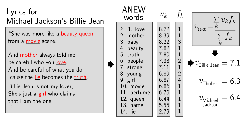
To estimate the overall valence score for a text, which we denote by $v_{\rm text}$, we (a) determine the frequency $f_{i}$ that the $i$th word from the ANEW study word list appears in the text; and (b) compute a weighted average of the valence of the ANEW study words as

$$v_{\rm text}=\frac{\sum_{i=1}^{n}v_{i}f_{i}}{\sum_{i=1}^{n}f_{i}}$$ (1)

where $v_{i}$ is the ANEW study’s recorded average valence for word $i$. As a simple example, take the pangram “The quick brown fox jumps over the lazy dog.” The three underlined words appear in the ANEW study word list with average valences 6.64, 4.38, and 7.57, respectively. We would therefore assign an overall valence score for the sentence of $v_{\rm text}=\frac{1}{3}$ $\times$ ($1\times$ 6.64 + $1\times$ 4.38 + $1\times$ 7.57) $\simeq 6.20$. We hasten to add that our method is only reasonable for large-scale texts where we can demonstrate robustness, and we discuss this in detail below. In Fig. 2, we also outline our measurement schematically, using the example of Michael Jackson’s lyrics. To give a sense of range, for the texts we analyse here, we find that average valence typically falls between 4.5 and 7.5 (our results for lyrics below will give concrete examples for these limiting values).

Our general focus is thus on quantifying how writings are received rather than on what an author may have intended to convey emotionally. Nevertheless, as we discuss below, we attempt to understand the latter with our investigations of blogs.

In using the ANEW data set, we also take the viewpoint that direct human assessment remains, in many complex contexts, superior to artificial intelligence methods. Describing the content of an image, for example, remains an extremely difficult computational problem, yet is trivial for people (von Ahn, 2006).

Since our method does not account for the meaning of words in combination, it is suitable only for large-scale texts. We argue that the results from even sophisticated natural language parsing algorithms (Riloff and Wiebe, 2003) cannot be entirely trusted for small-scale texts, as individual expression is simply too variable (Lee, 2004) and must therefore be viewed over long time scales (or equivalently via large-scale texts). Problematically, the desired scalability is a barrier for such parsing algorithms which run slowly and still suffer from considerable inaccuracy. With our method based on the ANEW data set, we are able to collect and rapidly analyze very large corpuses, giving strength to any statistical assessment. Indeed, with advances in cloud computing, we see no practical limit in the size of meaningful corpuses we can analyse.

A key aspect of our method is that it allows us to quantify happiness on a continuum. By comparison, previous analyses have focused on differences in frequency of words belonging to coarse, broad categories (Cohn et al., 2004), such as ‘negative emotion’, ‘no emotion’, and ‘positive emotion’. For example, using a category-based approach and covering a smaller scale in time and population size than we do here, studies of blogs over a single day have found that content and style vary with age and gender, suggesting automated identification of author demographics is feasible (Schler et al., 2006). However, comparisons between data sets using broad categorical variables are not robust, even if the categories can be ordered. Consider two texts that have the same balance of positive and negative emotion words. Without a value of valence for individual words, we are unable to distinguish further between these texts, which may easily be distinct in emotional content. By using the ANEW data set, we are able to numerically quantify emotional content in a principled way that can be refined with future studies of human responses to words.

II Description of large-scale texts studied

We use our method to study four main corpuses: song lyrics, song titles, blog sentences written in the first person and containing the word ‘feel’, and State of the Union addresses. Before exploring valence patterns in depth for these data sets, we first provide some summary statistics relevant to our particular interests, and we also detail our sources.

Counts	Song lyrics	Song titles	Blogs	SOTU∗
All words	58,610,849	60,867,223	155,667,394	1,796,763
ANEW words	3,477,575 (5.9%)	5,612,708 (9.2%)	8,581,226 (5.5%)	61,926 (3.5%)
Individuals	$\sim$ 20,000	$\sim$ 632,000	$\sim$ 2,335,000	43

^∗ SOTU = State of the Union addresses

Table 1: Total number of words in each corpus along with the number and percentage of words found in the ANEW database. Individuals refers to the number of distinct artists, blogs, and presidents.

Table 1 records the total number of words and ANEW words in each data set, along with the number of individual authors. The relative proportions of ANEW words within the four corpuses range from 3.5% (State of the Union) to 9.2% (song titles). These percentages are not insubstantial due to Zipf’s law (Zipf, 1949) and the high prevalence of articles, prepositions, etc., in language. Approximately 175 words account for half of all words in the British National Corpus, for example, with the five distinctly neutral words ‘the’, ‘of’, ‘and’, ‘a’, and ‘in’ comprising over 15%.

Rank	Song lyrics	Song titles	Blogs	SOTU∗
1	love (7.37%)	love (7.39%)	good (4.89%)	people (5.49%)
2	time (4.18%)	time (4.19%)	time (4.72%)	time (4.09%)
3	baby (2.75%)	baby (2.75%)	people (3.94%)	present (3.45%)
4	life (2.59%)	life (2.60%)	love (3.31%)	world (3.10%)
5	heart (2.14%)	heart (2.15%)	life (3.13%)	war (2.98%)

Table 2: Top five most frequently occurring ANEW words in each corpus with frequency expressed as a percentage of all ANEW words.

Table 2 shows the five most frequent ANEW words for each data set, presenting a kind of essence for each corpus. The top five words in song lyrics and titles (which we obtained from different databases, see below) are very similar in prevalence, with ‘love’ unsurprisingly being the dominant word. Blogs evince a more social aspect with ‘people’ and ‘life’ in the top five, while the nature of State of the Union addresses is reflected in the disproportionate appearance of ‘world’ and ‘war.’

Figure 3: Normalized frequency distribution of the ANEW study words binned by valence for the main corpuses (excluding song titles) we study here, along with the more specific example of Michael Jackson’s lyrics. Insets show ratios of normalized frequencies for corpuses to that of the ANEW study word set.

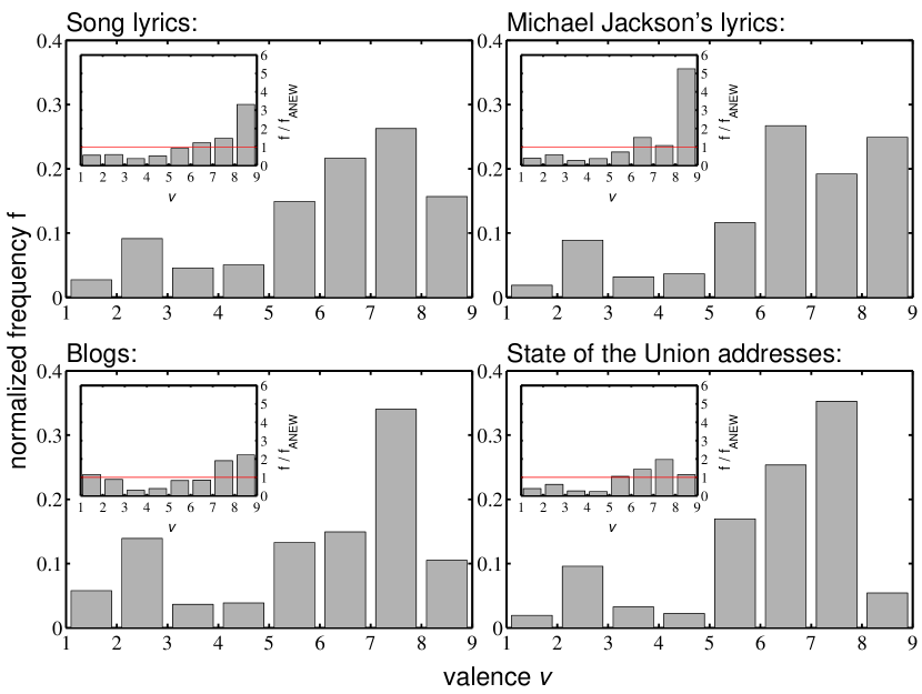
Fig. 3 shows the normalized abundances of ANEW study words appearing in our various corpuses, as a function of their average valence. We include the example of Michael Jackson’s lyrics for reference. The insets for each plot show the same distributions but now normalized by the underlying frequency distribution of ANEW words (Fig. 1). These insets reveal that song lyrics are weighted towards high valence words, and the mode bin is 8–9. Blogs, by contrast, have more low valence words resulting in a bimodal distribution, though the mode bin is again 8–9. State of the Union addresses favor high valence words in the 7–8 bin and show less negativity than blogs.

We obtained our four data sets as follows. We downloaded lyrics to $232,574$ songs composed by 20,025 artists between 1960 and 2007 from the website hotlyrics.net and tagged them with their release year and genre using the Compact Disc Data Base available online at freedb.org. We separately obtained from freedb.org a larger database of song titles and genre classifications. Starting August, 2005, first person sentences using the word feel (or a conjugated form) were extracted from blogs and made available through the website wefeelfine.org, via a public API (Harris and Kamvar, 2009). Demographic data was furnished by the site when available. These sentences appeared in over 2.3 million unique blogs during a 44 month span starting in August 2005. In total, we retrieved 9,563,128 sentences which appeared during the period August 26, 2005 to March 31, 2009, inclusive. For each day, we removed repeat sentences of six words or more to eliminate substantive copied material. We obtained State of the Union messages from the American Presidency Project at presidency.ucsb.edu. Finally, we accessed the British National Corpus at www.natcorp.ox.ac.uk.

III Results

Figure 4: A. Valence time series for song lyrics, showing a clear downward trend over the 47 year period starting in 1961. Valence is measured by averaging over the valences of individual words from the ANEW study (Bradley and Lang, 1999) found in songs released in each year. B. Box and whisker plot of relative valence time series for song lyrics for 1000 random sets of 750 ANEW words. The overall mean valence $v_{\rm avg}$ is removed from each time series for comparison; the inset histogram shows the distribution of overall means. Excluding the most frequent words such as ‘love’ (see Table 2) shifts the time series vertically but the downward trend remains apparent in all cases. Boxes indicate first and third quartiles and the median; whiskers indicate extent of data or 1.5$\times$interquartile range; and outliers are marked by a gray $\times$.

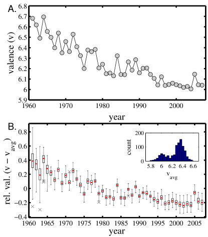
We analyse song lyrics first, in part to demonstrate the robustness of our approach. In Fig. 4A, we show how the average valence of lyrics declines from the years 1961 to 2007. The decline is strongest up until around 1985 and appears to level off after 1995. Since our estimate is based on a partial sample of all words, we need a way of checking its stability. In Fig. 4B, we repeat our analysis using 100 random subsets of the ANEW word list with 750 words, removing the overall average valence from each time series to facilitate comparison of the relative change of valence. The downward trend remains for each measurement while the overall average valence shifts (as shown by the inset). For example, as we have noted, love is the most frequent word in song lyrics, and with its high valence, its inclusion or exclusion from the measurement has the most significant impact on the overall average valence. Thus, we are confident that our estimates of relative as opposed to absolute valence are reasonable.

Figure 5: Valence Shift Word Graph: Words ranked by their absolute contributions to the drop in average valence of song lyrics from January 1, 1980 onwards relative to song lyrics from before January 1, 1980. The contribution of word $i$ is defined in Eq. (3) and explained in the surrounding text.

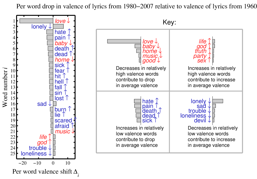
We more finely examine the reason for this decline in valence in Fig. 5 where we compare individual word prevalence changes in lyrics before and after 1980 using what we term a ‘Valence Shift Word Graph.’ For these graphs, we rank words by their descending absolute contribution to the change in average valence between the two eras, $\delta$. Word $i$’s contribution depends on its change in relative frequency, and its valence relative to the pre-1980 era average. In general, in comparing some text $b$ with respect to a given text $a$, we define the valence difference as

$$\delta(b,a)=v_{b}-v_{a}$$ (2)

and the percentage contribution to this difference by word $i$ as

$$\Delta_{i}(b,a)=100\times\frac{(p_{i,b}-p_{i,a})(v_{i}-v_{a})}{\delta(b,a)}$$ (3)

where $p_{i,a}$ and $p_{i,b}$ are the fractional abundances of word $i$ in texts $a$ and $b$. As required, summing $\Delta_{i}(b,a)$ over all $i$ gives +100% or -100% depending on whether $\delta(b,a)$ is positive or negative.

Four basic possibilities arise for each word’s contribution, as indicated by the key in Fig. 5. A word may have higher or lower valence than the average of text $a$, and it may also increase or decrease in relative abundance. Further, the contribution of word $i$ to $\Delta_{i}(b,a)$ will be 0 if either the relative prevalences are the same, or the average valence of word $i$ matches the average of text $a$. Note that $\Delta_{i}(b,a)$ is not symmetric in $b$ and $a$ and is meant only to be used to describe one text ($b$) with respect to another ($a$).

Ranking words according to the above definition of $\Delta_{i}$ gives us Fig. 5. We see that the decrease in average valence for lyrics after 1980 is due to a loss of positive words such as ‘love’, ‘baby’, and ‘home’ (italicized and in red) and a gain in negative words such as ‘hate’, ‘pain’, and ‘death’ (normal font and in blue). These drops are countered by the trends of less ‘lonely’ and ‘sad’, and more ‘life’ and ‘god’. The former dominates the latter and the average valence decreases from approximately 6.4 to 6.1. Even though the contribution of ‘love’ is clearly the largest, the overall drop is due to changes in many word frequencies. And while we are unable to assess words for which we do not have valence, we can make qualitative observations. For example, the word ‘not’, a generally negative word, accounts for 0.22% of all words prior to 1980 and 0.28% of all words after 1980, in keeping with the overall drop in valence.

Rank	Top Artists	Valence	Bottom Artists	Valence
1	All 4 One	7.15	Slayer	4.80
2	Luther Vandross	7.12	Misfits	4.88
3	S Club 7	7.05	Staind	4.93
4	K Ci & JoJo	7.04	Slipknot	4.98
5	Perry Como	7.04	Darkthrone	4.98
6	Diana Ross & the Supremes	7.03	Death	5.02
7	Buddy Holly	7.02	Black Label Society	5.05
8	Faith Evans	7.01	Pig	5.08
9	The Beach Boys	7.01	Voivod	5.14
10	Jon B	6.98	Fear Factory	5.15

Table 3: Average valence scores for the top and bottom 10 artists for which we have the lyrics to at least 50 songs and at least 1000 ANEW words.

Figure 6: Valence time series for song titles broken down by representative genres. For each genre, we have omitted years in which less than 1000 ANEW words appear.

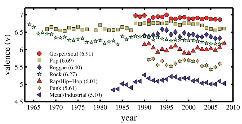
To help further unravel this decline in song lyric valence, we show the valence time series for some important music genres in Fig. 6. For this plot, we move to examining song titles for which we have a more complete data set involving genres. We observe that the valence of individual genres is relatively stable over time, with only rock showing a minor decrease. The ordering of genres by measured average valence is sensible: gospel and soul are at the top while several subgenres of rock including metal and punk, and related variants which emerged through the 1970’s exhibit much lower valences. Rap and hip-hop, two other notable genres that appear halfway through the time series, are lower in valence than the main genres of rock and pop, but not to the same degree as metal and punk. Thus, the decline in overall valence does not occur within particular genres, but rather in the evolutionary appearance of new genres that accessed more negative emotional niches. Finally, we show the top ten and bottom ten artists ranked according to valence in Tab. 3, given a certain minimum sampling of each artist’s lyrics.

While of considerable intrinsic interest, song lyrics of popular music provide us with a limited reflection of society’s emotional state, and we move now to exploring more directly the valence of human expression. The proliferation of personal online writing such as blogs gives us the opportunity to measure emotional levels in real time. As of June 23, 2008, the blog tracking website technorati.org reported it was following 112.8 million blogs. Blogger demographics are broad with an even split between genders and high racial diversity with some skew towards the young and educated (Lenhart and Fox, 2006).

We have examined nearly 10 million blog sentences retrieved via the website wefeelfine.org, as we have described in detail above. In focusing on this subset of sentences, we are attempting to use our valence measures not only to estimate perceived valence but also the revealed emotional states of blog authors. We are thus able to present results from what might be considered a very basic remote-sensing hedonometer.

Figure 7: Time series of average monthly valence for blog sentences starting with “I feel…” show a gradual upward trend over 3 years and 8 months. Notable individual days that differ strongly in valence from that of the surrounding month are indicated, including Christmas Day (trees), Valentine’s Day (hearts), 9/11 or 9/10 (squares), the US Presidential election and inauguration (circle and square), and Michael Jackson’s death (star). The gray bar at the top of the graph indicates the days for which we have data with white gaps corresponding to missing data (we have no estimate of valence for Christmas Day, 2006, hence its absence).

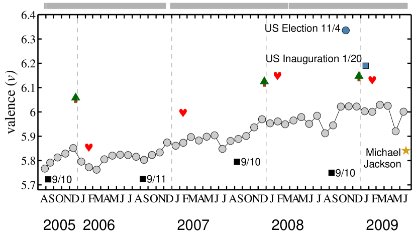
In Fig. 7, we plot average monthly valence as a function of time for blogs. We first see that over the time period examined, our subset of blog sentences gradually increase in valence, rising from an average of around 5.75 to over 6.0. Within individual years, there is generally an increase in valence over the last part of the year. In 2008, after a midyear dip, perhaps due to the economic recession, valence notably peaks in the last part of the year and appears to correlate with the US presidential election.

We highlight a number of specific dates which most sharply depart from their month’s average: Christmas Day; Valentine’s Day; September 11, 2006, the fifth anniversary of the World Trade Center and Pentagon attacks in the United States; the US Presidential Election, November 4, 2008; the US Presidential Inauguration, January 20, 2009; and the day of Michael Jackson’s death, June 25, 2009 (June 26 and 27 were also equally low).

Figure 8: Valence Shift Word Graphs for three example dates which are markedly different from the general valence trend shown in Fig. 7. The content of each date’s blogs is compared with that of the surrounding month. See Fig. 5 for an explanation of these graphs.

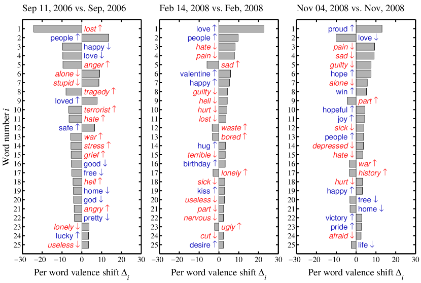
In Fig. 8, we show three Valence Shift Word Graphs corresponding to September 11, 2006; Valentine’s Day, 2008; and US Presidential Election Day, November 4, 2008. The first panel in Fig. 8 shows that the negative words most strongly driving down the average valence of the fifth anniversary of the 9/11 attacks are ‘lost’, ’anger’, ‘hate’, and ‘tragedy’ (‘terrorist’ ranks 10th in valence shift). The impact of these words is augmented by a decrease in frequency of ‘love’ and ‘happy’, overwhelming the appearance of more ‘people’ and less ‘stupid’ and ‘alone.’ In other years, September 10 rather than September 11 appears to be more clearly negative in tone, perhaps indicating an anticipatory aspect.

Christmas Day and Valentine’s Day are largely explained by the increase in frequency of the words Christmas and Valentine, both part of the ANEW word list. But other words contribute strongly. For Christmas Day, there is more ‘family’ and less ‘pain’, with an increase in ‘guilty’ going against the trend. As shown for Valentine’s day in 2008 in the second panel of Fig. 8, ‘love’ and ‘people’ are more prevalent, ‘hate’ and ‘pain’ less so, countervailed by more ‘sad,’ ‘lonely,’ and ‘bored.’

The strongest word driving the spike in valence for the 2008 US Election, the happiest individual day in the entire data set, is ‘proud’ (third panel of Fig. 8). Valence increases also due to a mixture of more positive words such as ‘hope’ and ‘win’ as well as a decrease in the appearances of ‘pain,’ ‘sad,’ and ‘guilty.’

Figure 9: A: Average valence as a function of blogger’s self-reported age. We use the age a blogger will turn in the year of his or her post and an approximately logarithmically growing bin size such that all data points are based on at least 3000 ANEW words. Bin boundaries are indicated by the dashed vertical lines. B: Average valence as a function of blogger’s absolute latitude. Bins are indicated by vertical gray lines. The first two bins have 8,390 and 26,071 ANEW words and the remainder all have approximately 10⁵ or more. C: Valence averaged over days of the week for blogs showing a subtle seven-day cycle peaking on Sunday with a trough in the middle of the week. Each day’s average is based on at least $10^{6}$ ANEW words.

Figure 10: Valence Shift Word Graph comparing bloggers who list themselves as turning 14 in year of post to those turning 45 to 60. The average valences are 5.55 and 5.98 respectively.

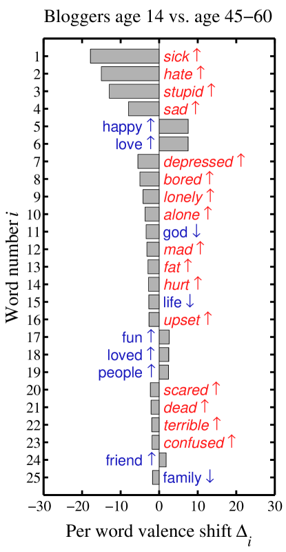
For some blogs, we also have self-reported demographic and contextual information allowing us to make some deeper observations. Fig. 9A shows that the average valence of blog sentences follows a pronounced single maximum, convex curve as a function of age. Thirteen and fourteen year-olds produce the lowest average valence sentences (5.58 and 5.55 respectively). As age increases, valence rises until leveling off near 6.0 for ages 45–60, and then begins to trend downwards. Fig. 10 compares 14 year-olds to those of age 45–60, and we see the former disproportionately using low valence words ‘sick’, ‘hate’, ‘stupid’, ‘sad’, ‘depressed’, ‘bored’, ‘lonely’, ‘mad’, and ‘fat.’ The increase is most marked throughout the teenage years with 20 year-olds (5.83) closer in average valence to 45–60 year-olds than to 14 year-olds. At the other end of the age spectrum, individuals in the 75 to 84 age range produce sentences with valence similar to those of 17 year olds.

Our age dependent estimates of valence comport with and extend previous observations of blogs that suggested an increase in valence over the age range 10–30 (Schler et al., 2006). Our results are however at odds with those of studies based on self-reports which largely find little or no change in valence over life times (Easterlin, 2001, 2003). These latter results have been considered surprising as a rise and fall in valence—precisely what we find here—would be expected due to changes in income (rising) and health (eventually declining) (Easterlin, 2001). Our results do not preclude that self-perception of happiness may indeed be stable, but since our results are based on measured behavior, they strongly suggest individuals do present differently throughout their lifespan. And while we have no data regarding income, because income typically rises with age, our results are sympathetic to recent work that finds happiness increases with income (Stevenson and Wolfers, 2008), going against the well known Easterlin Paradox, popularized as the notion that ‘money does not buy happiness’ (Easterlin, 1974).

Fig. 9B shows that the average valence of blog sentences gently rolls over as a function of absolute latitude (i.e, combining both the Northern and Southern Hemispheres). Average valence ranges from 5.71 (for 0 to 11.5 degrees) up to 5.83 (for 29.5 to 44.5 degrees) and then back to 5.78 (for 52.5 to 69.5 degrees). Seasonal Affective Disorder (Rosenthal et al., 1984) may be the factor behind the small drop for higher latitudes, though a different mechanism would need to be invoked to account for lower valence near the equator. One possible explanation could be that the relatively higher population of the mid-latitudes leads to stronger social structures (Layard, 2005). We find some support for the social argument for individuals near the equator (absolute latitude $\leq 11.5$), who we observe more frequently use the words ‘sad’, ‘bored’, ‘lonely’, ‘stupid’ and ‘guilty’ and avoid using ‘good’ and ‘people.’ On the other hand, the valence drop at higher latitudes (between 52.5 and 69.5 degrees absolute latitude) is reflected in the frequency changes of a mixture of social, psychological, and some conditions-related words: ‘sick’, ‘guilty’, ‘cold’, ‘depressed’, and ‘headache’ all increase, ‘love’ and ‘life’ decrease, offset by less ‘hurt’ and ‘pain’ and more ‘bed’ and ‘sleep.’

At a much more subtle level, a weekly cycle in valence is visible in blog sentences (Fig. 9C). A relatively sharp peak in valence occurs on Sunday, after which valence steadily drops daily to its lowest point on Wednesday before climbing back up. Monday, contrary to commonly held perceptions but consistent with previous studies (Stone et al., 1984), exhibits the highest average valence after Sunday, perhaps indicating a lag effect.

We also observe some variation among countries. Of the four countries with at least 1% representation, the United States has the highest average valence (5.83) followed by Canada (5.78), the United Kingdom (5.77), and Australia (5.74).

In terms of gender, males exhibit essentially the same average valence as females (5.89 versus 5.91). Females however show a larger variance than males (4.75 versus 4.44) in agreement with past research (Snyder and Lopez, 2009). We further find females disproportionately use the the most impactful high and low valence words separating the two genders: ‘love’, ‘baby’, ‘loved’ and ‘happy’ on the positive end, and ‘hurt’, ‘hate’, ‘sad’, and ‘alone’ on the negative end. In fact, of the top 15 words contributing to $\delta({\rm female},{\rm male})$, the only one used more frequently by males is ‘good.’

Figure 11: Average valence of State of the Union addresses, binned by President and plotted against the average of the years the President was in office.

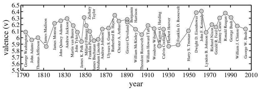
We turn to our last data set, State of the Union (SOTU) addresses for the United States. These addresses, which include both speeches and written reports, grant us a starting point for assessing the emotional temperature of the United States over its 220 year history, as may or may not have been intended by the authors. Fig. 11 shows a valence time series for SOTU addresses binned by President. In comparison to our lyrics and blog data sets, SOTU addresses comprise far fewer words and the observations we make are consequently tempered. Nevertheless, we do find some resonance between the valence level of SOTU addresses and major historical events.

The presidents with the highest average valence scores are Kennedy (6.41), Eisenhower (6.38), and Reagan (6.38), all of whose speeches are tightly clustered around their means. Eisenhower and Kennedy reach a high point after a period of relatively low valence starting with the First World War through and beyond which Wilson’s speeches steeply drop from an initial 6.58 in 1913 to 5.88 in 1920. The mean valence of Coolidge’s addresses provide the single exception during this time. Coolidge’s successor Hoover’s low average is largely due to his speech in 1930, the first one given after the stock market crash of October 29, 1929—Black Tuesday—which marked the beginning of the Great Depression; his speeches are burdened with ‘depression’, ‘debt’, ‘crisis’, and ‘failure.’ While Franklin Roosevelt’s overall average valence is low, the first eight of his four term stay in office range from 6.06 to 6.34. His last four speeches, coming during the Second World War (1942–1945), are sharply lower in valence, ranging from 5.48 to 5.60; ‘war’ naturally dominates these later speeches and along with ‘fight’ and ‘destroy’, overwhelm the positives of ‘peace’ and ‘victory.’

The large-scale pattern of the 19th Century shows two periods of relatively high valence, 1820–1840 and 1880–1890. The years before and during the American Civil War form a local minimum in valence corresponding to Buchanan and Lincoln.

The recent era shows a drop from Eisenhower and Kennedy’s level to that of Johnson (6.08), the latter’s first SOTU speech coming just seven weeks after the assassination of Kennedy, and the remainder through the heightening Vietnam War. Valence rises through the 1970’s to reach the high of Reagan in the 1980’s, from which it has since declined.

IV Concluding remarks

Undoubtedly, the online recording of social interactions and personal experiences will continue to grow, providing ever richer data sets and the consequent opportunity and need for a wide range of scientific investigations. A natural extension of our work here would be to examine the dynamics of emotions in online interactive contexts, particularly in the realm of contagion (Hatfield et al., 1993; Fowler and Christakis, 2008). If emotional contagion is observable, we would then be in a position to characterize its nature on the spectrum from analogous to an infectious disease (Murray, 2002) to the more complex threshold-based contagion (Granovetter, 1978; Dodds and Watts, 2004). Our technique could also be useful in testing predictive theories of social interactions such as Heise’s affect control theory (Heise, 1979) and Burke’s identity control theory (Stets and Tsushima, 2001).

While we have been able to make and support a range of observations with our method for measuring the emotional content of large-scale texts, our approach can be improved in a number of ways. A first step would be to perform experiments and surveys to gather emotional content estimates for a more extensive set of individual words. The instrumental lens can also be made more sophisticated by coupling word assessments with detailed demographics of participants. Other approaches not necessarily based on semantic differentials in the manner of the ANEW study could also be naturally explored. Game-based experiments could also be used to assess the emotional content of common word groups and phrases (von Ahn, 2006), allowing us to better characterize the micro-macro connection between the atoms of words and sentences, and differences in interpretations among various age groups and cultures.