On the Braess Paradox
with Nonlinear Dynamics and Control Theory

Abstract.

We show the existence of the Braess paradox for a traffic network with nonlinear dynamics described by the Lighthill–Whitham-Richards model for traffic flow. Furthermore, we show how one can employ control theory to avoid the paradox. The paper offers a general framework applicable to time-independent, uncongested flow on networks. These ideas are illustrated through examples.

1. Introduction

Consider the following scenario: We have a simple network consisting of two routes connecting $A$ to $B$, see Figure 1.

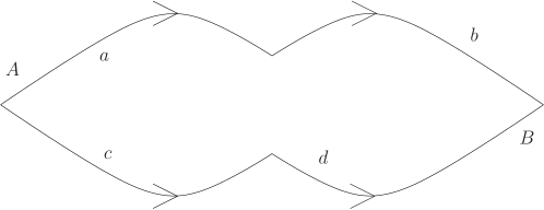
Figure 1. Network consisting of two routes connecting $A$ to $B$. The route $\alpha$ consists of the roads $a$ and $b$, the route $\beta$ consists of the roads $c$ and $d$.

Each route consists of two roads. Roads $a$ and $d$ are identical, as are roads $b$ and $c$. Traffic is unidirectional in the direction from $A$ to $B$. Travel time along roads $a$ and $d$ are given by $\rho/100$, where $\rho$ is the number of vehicles on that road, while the travel time is $45$ for each of roads $b$ and $c$, irrespective of the number of vehicles on that road. In equilibrium, vehicles will distribute evenly between the two routes connecting $A$ and $B$, i.e., roads $a$ & $d$ and $b$ & $c$. Assuming that initially $m=4000$ vehicles start from $A$, we find a travel time of $65$ along each of the two routes. Add a road $e$ as given in Figure 2, and assume that the travel time is zero along this road.

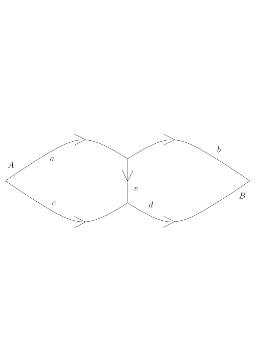
Figure 2. A network consisting of three routes $\alpha$, $\beta$, and $\gamma$ connecting $A$ to $B$. The route $\alpha$ comprises the roads $a$ and $b$, the route $\beta$ comprises the roads $c$ and $d$ and, finally, the route $\gamma$ consists of the roads $a$, $e$, and $d$.

Drivers will start using the new road, reducing their travel time from $65$ to $40$. However, as more and more drivers use the new road, their travel time will increase to $80$. Now, no driver will have an incentive to use the old roads, i.e., avoiding road $e$, as the travel time along those roads will be $85$. Thus all drivers are worse off than before, in spite of having a new road. This is the Braess paradox in a nutshell: Adding a new road to a network may make travel times worse for all. In both cases the equilibrium is a Wardrop equilibrium (i.e., all routes used have the same travel time, and all unused routes have longer travel times) as well as a Nash equilibrium.

This is the simplest example of the Braess paradox, introduced (with a different example) by Braess in 1968 [3], see also [18]. This example and some generalizations have been studied in, e.g., [10, 12, 23]. In spite of the unrealistic assumptions in the prevalent example above, the paradox has turned out to be ubiquitous and intrinsic to dynamical networks. The paradox also appears in other situations not modeling traffic flow [24], see, e.g., [19] for an example involving mesoscopic electron systems, and [7] for an example with mechanical springs. Furthermore, the paradox can be reformulated in the context of game theory. In addition, there are well documented examples of the paradox occurring in real-life traffic situations, e.g., in Seoul [2] and Stuttgart [15, pp. 57–59], see also [27]. Not surprisingly, the paradox has been well described also in general media, see, e.g., [16, 1, 25] and on Wikipedia as well as YouTube. The extensive discussion about the Braess paradox makes a complete reference list impossible, see, however, [9, 21, 22]. In this paper we only refer to articles directly related to the research at hand.

Here we want to study the Braess paradox with a more realistic nonlinear dynamics. More specifically, we want to model unidirectional traffic along roads by a macroscopic model where only densities of vehicles are considered. We believe this to be novel. In this class of models, introduced by Lighthill–Whitham [17] and Richards [20] (hereafter denoted the LWR model), vehicles, described by a density $\rho$ rather than individually, drive with a velocity determined by the density alone; higher density yields slower speed while low density lets vehicles approach the speed limit. At a maximum density with bumper-to-bumper vehicles, traffic comes to a halt. The dynamics is well described by the nonlinear partial differential equation

(1.1) $$\partial_{t}\rho+\partial_{x}\left(\rho\,v(\rho)\right)=0,$$

see, e.g., [14, pp. 11–18]. The function $q(\rho)=\rho v(\rho)$ is denoted the flux function, or, in the context of traffic flow, the fundamental diagram. It is in general a concave function that equals zero when $\rho$ vanishes and when $\rho$ equals the maximum possible road density. Hyperbolic conservation laws, as equations of the type (1.1) are called, have been used to study traffic on a network, starting with Holden and Risebro [13], see, e.g., the book by Garavello and Piccoli [11]. Related results on a game theoretic approach to network traffic through the LWR model, see [4, 5]. For general theory concerning hyperbolic conservation laws we refer to [14].

However, the Braess paradox describes an equilibrium situation, and it is not relevant to include time variation. Rather, we want to study stationary solutions where the velocity is a given function of the density of vehicles on the road. At a junction, the differential equation (1.1) will in general, if the two roads have different properties, establish a complicated wave pattern, creating waves that emanate from the junction in both directions. However, in the equilibrium situation, this cannot happen, as it would create time-dependent waves. Thus, we will set up the example in such a way that no waves are created at junctions.

In this paper we analyze the same simple network as described above, but with much more realistic dynamics. More general examples are of course possible using the same methods. However, calculations become more cumbersome and less transparent, and we here focus on presenting the ideas of the model, exemplified on the simple network in Figures 1 and 2. For another approach to the Braess paradox, see, e.g., [8].

The prevalence of the Braess paradox is unwanted, and one would like to take measures to prevent its occurrence. In the example in the present paper, we use the velocity of the road $e$ as a control parameter. By properly adjusting the speed limit on road $e$, one can force the Braess paradox to disappear, and make the social optimum coincide with the Nash equilibrium.

This can be illustrated in the simple example in the beginning of the introduction. Given a “benevolent dictator” who wants to reduce the total travel time and reach the social optimum, a short calculation shows that, with $m=4000$, 1750 vehicles should follow each of the routes $a$ & $b$ and $c$ & $d$, and the remaining $500$ vehicles should follow the route $a$, $e$, and $d$. Although a social optimum, this situation is neither a Wardrop nor a Nash equilibrium.

This paper offers a framework applicable to general networks. The input is, in addition to the network itself, the length and velocity fields of each road as well as the influx. We assume that traffic is in the uncongested, or free, phase. This will prevent waves from emanating from the junctions.

2. A dynamic version of the Braess paradox

2.1. Notation and basic definitions

Below, we denote ${\mathbb{R}}^{+}=[0,+\infty)$ and $S^{n}=\{\vartheta\in[0,1]^{n}\mid\sum_{j}\vartheta_{j}\leq 1\}$ is the standard simplex in ${\mathbb{R}}^{n}$. The sphere centered at $\vartheta$ with radius $r$ is denoted by $B_{r}(\vartheta)$.

Two points $A$ and $B$ are connected through a network of roads. Along each road, traffic is described through the LWR model (1.1). At each junction, the total flow exiting the junction equals the incoming one, so that the total quantity of vehicles is conserved.

The macroscopic description obtained solving (1.1) along each road also provides the full microscopic portrait of the network. Indeed, once $\rho=\rho(t,x)$ is known along the road $r$ connecting, say, the junction at $A$ to that at $B$, the single vehicle leaving from $A$ at time $t_{o}$ travels along $r$ according to

(2.1) $$\left\{\begin{array}[]{l}\dot{x}=v\big{(}\rho(t,x(t))\big{)},\\ x(t_{o})=A\,.\end{array}\right.$$

The travel time $\tau_{r}(t_{o})$ along the road $a$ is then implicitly defined by

(2.2) $$x\left(\tau_{r}(t_{o})\right)=B\,.$$

To compute $\tau_{r}(t_{o})$, in general, one has first to provide (1.1) with initial and boundary data, then solve the resulting initial-boundary value problem to obtain $\rho=\rho(t,x)$, use this latter expression to solve the ordinary differential equation (2.1) and finally solve the equation (2.2). Observe that the right-hand side in the ordinary differential equation in (2.1) is in general discontinuous, nevertheless in the present setting it is well-posed, see [6]. In the present stationary framework, this procedure can be pursued explicitly, as we detail below in Example 2.6. Remark that, in a stationary regime, all travel times are independent of the starting time $t_{o}$.

For the above travel times to be a reliable measure of the network efficiency, it is necessary that they are independent from any particular initial data. Also the standard initial-boundary value problem for (1.1) with zero initial density on the whole network is unsatisfactory, since it would give results that depend on the transient period necessary to fill the network. We are thus bound to select stationary solutions, assigning a constant inflow at $A$ for all times $t\in{\mathbb{R}}$. Moreover, to allow for stationary solutions, we also assume that the total flow incoming at any junction never exceeds the total capacity of the roads exiting that junction.

In the general LWR model (1.1), the flux function $q=q(\rho)$ is a concave function that vanishes at zero density and at $\rho_{M}$, the maximum density. The flux has a unique maximum for some value $\rho_{m}\in(0,\rho_{M})$. As usual, we refer to densities below $\rho_{m}$ as the uncongested, or free, phase, and for densities above $\rho_{m}$ as the congested phase. In the remaining part of the paper, to obtain stationary solutions, we need to remain in the free phase only, so that $\rho\in[0,\rho_{m}]$ throughout the network. In order to simplify the notation we will use the normalization $\rho_{m}=1$ for all roads. We will not make any assumptions on, or reference to, $q$ above this value. Hence, on the flow function we pose the following assumption:

(q):

$q\in\mathbf{C^{3}}([0,1];{\mathbb{R}}^{+})$, $q(0)=0$, $q^{\prime}>0$ and $q^{\prime\prime}\leq 0$.

Clearly, if $q$ satisfies (q), then the speed law $v(\rho)=q(\rho)/\rho$ is well-defined, continuous, strictly positive and weakly decreasing, see Lemma A.1. As a result, the travel along a road segment is a convex and increasing function of the inflow.

Lemma 2.1.

Let $q$ satisfy (q) with $q^{\prime\prime\prime}\leq 0$ and call $\varphi=q(1)$. Then, the travel time $\tau(\vartheta)$, which is defined by $x\left(\tau(\vartheta)\right)=B$ where

$$\mbox{ $x$ solves}\quad\begin{cases}\dot{x}=v\left(\rho(t,x(t))\right),\\ x(0)=A,\end{cases}\quad\mbox{ and }\quad\mbox{$\rho$ solves}\quad\begin{cases}\partial_{t}\rho+\partial_{x}q(\rho)=0,\\ q\left(\rho(t,A)\right)=\vartheta\varphi,\end{cases}$$

is of class $\mathbf{C^{2}}([0,1];{\mathbb{R}}^{+})$, weakly increasing and convex.

The proof follows directly from Lemma A.3.

When $\gamma$ is a route consisting of the adjacent roads $r_{1},r_{2},r_{3},\ldots$, the travel time $\tau_{\gamma}(t_{o})$ along $\gamma$ is then defined as the sum $\sum_{i}\tau_{r_{i}}$ of the travel times of all roads.

A network consists of several routes connecting $A$ to $B$. To describe it, we enumerate each single road (or edge) and construct the matrix $\Gamma$ setting

$$\Gamma_{ij}=\begin{cases}1&\text{the road $r_{i}$ belongs to the route $\gamma_{j}$},\\ 0&\text{otherwise.}\end{cases}$$

We now assign a constant total inflow $\varphi$ at $A$ and call $\vartheta_{i}$ the fraction of the drivers that reach $B$ along the route $\gamma_{j}$.

A single road may well belong to more than one route, so that the flow along the road $r_{i}$ is $\varphi\Gamma_{i}\vartheta=\varphi\sum_{i}\Gamma_{ij}\vartheta_{j}$ and the travel time along that road results to be $\tau_{r_{i}}(\Gamma_{i}\vartheta)$. The total travel time $\tau_{i}$ along the $i$th route is in general a function of all partition parameters, more precisely

$$\tau_{\gamma_{j}}(\vartheta)=\sum_{i}\Gamma_{ij}\;\tau_{r_{i}}\!(\Gamma_{i}\vartheta).$$

From a global point of view, it is natural to evaluate the quality of a network through the mean global travel time $T(\vartheta)=\sum_{j}\vartheta_{j}\,\tau_{\gamma_{j}}(\vartheta)$ or, using matrix notation $\tau_{r}(\Gamma\vartheta)=[\tau_{r_{1}}(\Gamma_{1}\vartheta)\,\cdots\,\tau_{r_{n}}(\Gamma_{n}\vartheta)]$, we find

(2.3) $$T(\vartheta)=\tau_{r}(\Gamma\vartheta)\;\Gamma\;\vartheta\,.$$

We call globally optimal a state $\vartheta_{G}\in S^{n}$ that minimizes $T$ over $S^{n}$, i.e., $\vartheta_{G}=\operatorname{argmin}_{\vartheta\in S^{n}}T(\vartheta)$. This social optimum state conforms to Wardrop’s Second principle, see [26, p. 345].

Proposition 2.2.

Let all road travel times $\tau_{r_{1}},\ldots,\tau_{r_{m}}$ be of class $\mathbf{C^{2}}([0,1];{\mathbb{R}}^{+})$, weakly increasing and convex. Then, the map $T$ is in $\mathbf{C^{2}}([0,1];{\mathbb{R}}^{+})$ is convex.

The proof is deferred to the Appendix.

For brevity, we call relevant those travel times $\tau_{i}$ such that $\vartheta_{i}\neq 0$.

Definition 2.3.

A state $\bar{\vartheta}\in S^{n}$ is an equilibrium state if all relevant travel times coincide, i.e., for all $i,j\in\{1,\ldots,n\}$

$$\mbox{ if }\bar{\vartheta}_{i}\neq 0\mbox{ and }\bar{\vartheta}_{j}\neq 0,\mbox{ then }\tau_{i}(\bar{\vartheta})=\tau_{j}(\bar{\vartheta})=\bar{\tau}\,,$$

the common value $\bar{\tau}$ of the travel times being the equilibrium time.

In other words, at equilibrium all drivers need the same time to go from $A$ to $B$. A common criterion for optimality goes back to Pareto.

Definition 2.4.

An equilibrium state $\vartheta^{P}\in S^{n}$ is a local Pareto point if there exists a positive $\delta$ such that for all $\vartheta\in B_{\delta}(\vartheta^{P})\cap S^{n}$ if there exists a $j$ such that $\tau_{\gamma_{j}}(\vartheta)<\tau_{\gamma_{j}}(\vartheta^{P})$, then there exists also a $k$ such that $\tau_{\gamma_{k}}(\vartheta)>\tau_{\gamma_{k}}(\vartheta^{P})$.

In other words, no (small) perturbation of a Pareto point may reduce all travel times.

However, from a “selfish” point of view, each driver aims at reducing his/her own travel time. It is then natural to introduce the following definition.

Definition 2.5.

An equilibrium state $\vartheta^{N}\in S^{n}$ is a local Nash point if there exists a positive $\delta$ such that for all $\varepsilon\in(0,\delta]$ and all $j,k=1,\ldots,n$,

$$\mbox{if }\vartheta^{N}+\varepsilon e_{j}-\varepsilon e_{k}\in S^{n}\mbox{, then }\tau_{\gamma_{j}}(\vartheta^{N}+\varepsilon e_{j}-\varepsilon e_{k})>\tau_{\gamma_{k}}(\vartheta^{N})\,,$$

where $e_{j}$ is the unit vector directed along the $j$th axis.

In other words, it is not convenient for $\varepsilon$ drivers to change from route $k$ to route $j$, for any $j,k=1,\dots,n$.

Example 2.6.

Consider the simple case of the network in Figure 3, and assume that its dynamics is described as follows:

Road	Length	Density	Model	Flow
$a$	$3/2$	$\rho$	$\partial_{t}\rho+\partial_{x}\left(\rho\,v(\rho)\right)=0$	$q(\rho)=\left(-1+\sqrt{1+8\rho}\right)/4$
$b$	$1$	$R$	$\partial_{t}R+\partial_{x}\left(R\,V(R)\right)=0$	$Q(R)=-1+\sqrt{1+R}$

The maximal inflow $\varphi$ at $A$ that, for any $\vartheta\in[0,1]$, can be partitioned in $\vartheta\,\varphi$ along $a$ and $(1-\vartheta)\varphi$ along $b$ is $\min\left\{q(1),Q(1)\right\}=\sqrt{2}-1$.

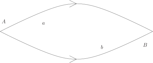
Figure 3. A simple network connecting $A$ to $B$ where the globally optimal state differs from the Nash optimal one.

With this constant inflow as left boundary data in (1.1), the resulting (stationary) densities are

$$\text{$\rho=(1+2\,\vartheta\,\varphi)\,\vartheta\,\varphi$ along road $a$, and $R=\left(2+(1-\vartheta)\varphi\right)(1-\vartheta)\,\varphi$ along road $b$}\,.$$

The corresponding constant traffic speeds

$$\text{$v(\rho)=(1+2\,\vartheta\,\varphi)^{-1}$ along road $a$, and $V(R)=(2+(1-\vartheta)\varphi)^{-1}$ along road $b$},$$

inserted in (2.1), lead to the following travel times on the two roads:

$$\text{$\tau_{a}(\vartheta)=3(1+2\,\vartheta\,\varphi)/2$ along road $a$, and $\tau_{b}(1-\vartheta)=2+(1-\vartheta)\varphi$ along road $b$}\,.$$

Finally, the mean global travel time defined at (2.3) is

$$T(\vartheta)=2+\varphi-\frac{1+4\,\varphi}{2}\,\vartheta+4\,\vartheta^{2}\,\varphi\,.$$

According to Definition 2.5, we have a unique Nash point at $\vartheta^{N}$ and a unique globally optimal state at $\vartheta_{G}$, where

$$\vartheta^{N}=\begin{cases}0,&\varphi\in[0,1/6),\\ \frac{1+2\,\varphi}{8\,\varphi},&\varphi\in[1/6,\sqrt{2}-1],\end{cases}\qquad\vartheta_{G}=\begin{cases}0,&\varphi\in[0,1/12),\\ \frac{1+4\,\varphi}{16\,\varphi},&\varphi\in[1/12,\sqrt{2}-1].\end{cases}$$

Clearly, $\vartheta^{N}$ is also a Pareto point according to Definition 2.4. Note that the globally optimal state may well differ from the Nash optimal one and both depend on the total inflow $\varphi$, see Figure 4.

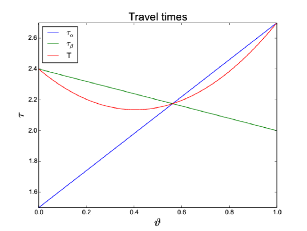
Figure 4. Travel times of the situation described in Example 2.6 with $\varphi=0.4$, so that $\vartheta^{N}=0.5625$ and $\vartheta_{G}=0.40625$.

2.2. The case of four roads

Consider the network in Figure 1. The network is given by two routes, denoted $\alpha$ and $\beta$, connecting $A$ and $B$. The route $\alpha$ consists of roads $a$ and $b$, the route $\beta$ consists of roads $c$ and $d$. Roads $a$ and $d$ have the same length $\ell$ and the same fundamental diagram $q$. Similarly, roads $b$ and $c$ share the same length $L$ and the same flow density relation. Traffic is always assumed to be unidirectional from $A$ to $B$, and no obstructions, e.g., traffic lights, are encountered at the junctions.

Along each road, the dynamics of traffic is described by the LWR model (1.1) with flux functions that lead to the travel times

$$\tau_{a}(\vartheta)=\tau_{d}(\vartheta)\quad\mbox{ and }\quad\tau_{b}(\vartheta)=\tau_{d}(\vartheta)\,,$$

so that the travel time $\tau_{\alpha}(\vartheta)$ along the route $\alpha$ and $\tau_{\beta}(1-\vartheta)$ along the route $\beta$, are

$$\tau_{\alpha}(\vartheta)=\tau_{a}(\vartheta)+\tau_{b}(\vartheta)\quad\mbox{ and }\quad\tau_{\beta}(1-\vartheta)=\tau_{a}(1-\vartheta)+\tau_{b}(1-\vartheta)\,.$$

Then, $\vartheta\mapsto\tau_{\alpha}(\vartheta)$ is (weakly) increasing, while $\vartheta\mapsto\tau_{\beta}(1-\vartheta)$ is (weakly) decreasing. Since $\tau_{\alpha}(1/2)=\tau_{\beta}(1/2)$, we have that $\vartheta^{N}=1/2$ is a Nash (and also Pareto) point for this system. It is easy to verify that $(\vartheta^{N},\vartheta^{N})$ is also globally optimal, since it is the argument that minimizes $T(\vartheta_{1},\vartheta_{2})$ over the simplex $S^{2}$.

2.3. The case of five roads

We now introduce a new road in Figure 1, passing to the network described in Figure 2. The new road $e$, which has the direction from $a$ to $d$, has length $\tilde{\ell}$ and its dynamics is characterized by a flow function $\tilde{q}$ satisfying (q). The presence of the road $e$ allows us to consider the route $\gamma$ connecting $A$ to $B$ consisting of the roads $a$, $e$, and $d$. For all $\vartheta_{1},\vartheta_{2}\in[0,1]$ such that $\vartheta_{1}+\vartheta_{2}\leq 1$, we now let the inflow $\vartheta_{1}\,\varphi$ enter $\alpha$, $\vartheta_{2}\,\varphi$ enter $\beta$ and the remaining $(1-\vartheta_{1}-\vartheta_{2})\,\varphi$ enter $\gamma$. The travel times along the three routes are then:

(2.4) $$\tau_{\alpha}(\vartheta_{1},\vartheta_{2}) =\tau_{a}(1-\vartheta_{2})+\tau_{b}(\vartheta_{1}),$$

$$\tau_{\beta}(\vartheta_{1},\vartheta_{2}) =\tau_{b}(\vartheta_{2})+\tau_{a}(1-\vartheta_{1}),$$

$$\tau_{\gamma}(\vartheta_{1},\vartheta_{2}) =\tau_{a}(1-\vartheta_{2})+\tau_{e}(1-\vartheta_{1}-\vartheta_{2})+\tau_{a}(1-\vartheta_{1})\,.$$

Observe that $\tau_{\alpha}(\vartheta,\vartheta)=\tau_{\beta}(\vartheta,\vartheta)$.

The mean global travel time is

(2.5) $$T(\vartheta_{1},\vartheta_{2})=\vartheta_{1}\,\tau_{\alpha}(\vartheta_{1},\vartheta_{2})+\vartheta_{2}\,\tau_{\beta}(\vartheta_{1},\vartheta_{2})+(1-\vartheta_{1}-\vartheta_{2})\,\tau_{\gamma}(\vartheta_{1},\vartheta_{2})\,.$$

2.4. The Braess paradox

We now compare the travel times obtained in the two cases described by Figures 1 and 2. To this end, observe that the travel times $\tau_{\alpha}^{\rm IV}$ and $\tau_{\beta}^{\rm IV}$ in the case of four roads, and referring to Figure 1, are obtained from those in the $5$ roads case setting

$$\tau_{\alpha}^{\rm IV}(\vartheta)=\tau_{\alpha}(\vartheta,1-\vartheta)\quad\mbox{ and }\quad\tau_{\beta}^{\rm IV}(\vartheta)=\tau_{\beta}(\vartheta,1-\vartheta).$$

Theorem 2.7.

Let the travel times $\tau_{a},\tau_{b},\tau_{e}\in\mathbf{C^{0}}([0,1];{\mathbb{R}}^{+})$ be non decreasing and assume that $\tau_{a}$ or $\tau_{b}$ are not constant. If the travel times defined in (2.4) satisfy

(2.6) $$\tau_{\alpha}(1/2,1/2)<\tau_{\gamma}(0,0)<\tau_{\alpha}(0,0),$$

then:

• $\vartheta^{N}\equiv(0,0)$ is the unique local Nash point for the network with five roads in Figure 2;

• the corresponding equilibrium time $\tau_{\gamma}(0,0)$ is worse than the globally optimal configuration for the network with four roads in Figure 1.

Under the above conditions we have the occurrence of the Braess paradox.

Observe that the point $\vartheta^{P}\equiv(1/2,1/2)$ is the unique Pareto point for the five roads networks.

Condition (2.6) allows us to construct several examples illustrating the Braess paradox.

Example 2.8.

With the notation in Figure 2, choose

$$\begin{array}[]{cccr@{\,}c@{\,}lr@{\,}c@{\,}l}\mbox{Road}&\mbox{Length}&\mbox{Density}&\mbox{Flow}&\\ a,\,d&1&\rho&q(\rho)&=&\ln(1+\rho)\\ b,\,c&1&R&Q(R)&=&R\,V&(V&\in&{\mathbb{R}})\\ e&1&\tilde{\rho}&\tilde{q}(\tilde{\rho})&=&\tilde{\rho}\,\tilde{v}&(\tilde{v}&\in&{\mathbb{R}})\end{array}$$

Condition (2.6) then becomes

$$\frac{e^{\varphi}-1}{\varphi}<\frac{1}{V}-\frac{1}{\tilde{v}}<\frac{2}{\varphi}(e^{\varphi}-e^{\varphi/2}),$$

and, for any $\varphi\in\left(0,\min\{\ln 2,V,\tilde{v}\}\right]$, it can easily be met for suitable $V$, $\tilde{v}$, see Figure 5.

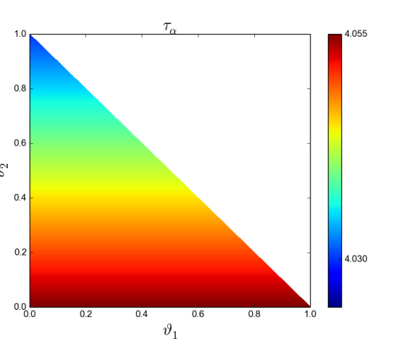
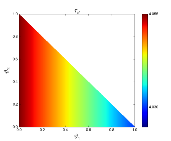
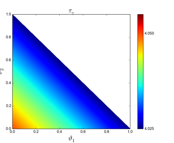
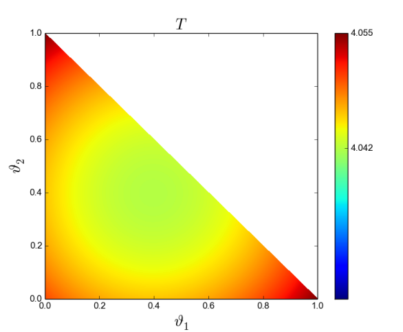
Figure 5. Contour plots of the travel times related to Example 2.8 with $V=0.33$, $\tilde{v}=0.5$, $\ell=L=\tilde{\ell}=1$, $\varphi=0.05$. Above, $\tau_{\alpha}$ and $\tau_{\beta}$; below $\tau_{\gamma}$ and the global travel time $T$. The color scales to the right are the same in all figures and display the maximal and minimal values of the diagrams to their left.

3. Control theory for the novel road — or how to cope with the Braess paradox

Our next aim is proving that in the case of the network in Figure 2, a carefully chosen speed limit imposed on the novel road $\gamma$ makes the Nash optimal state coincide with the globally optimal one.

We use the same notation as in Section 2.4, but we use the travel time $\tilde{\tau}$ along the $e$ road as control parameter. Equivalently, we impose that the speed along the road $\gamma$ is $\tilde{v}$, so that

(3.1) $$\tau_{e}(\vartheta_{1},\vartheta_{2})=\tilde{\tau}.$$

The next theorem says that there exists an optimal control.

Theorem 3.1.

Let the travel time $\tau_{a},\tau_{b}\in\mathbf{C^{0}}([0,1];{\mathbb{R}}^{+})$ be non decreasing and convex, one of the two being strictly convex. Then, there exists a constant travel time $\tilde{\tau}\in{\mathbb{R}}^{+}$ such that the network in Figure 2 admits a partition $(\vartheta_{*},\vartheta_{*})$ which is a Nash optimal state and also globally minimizes the mean global travel time.

Thus, by carefully selecting the travel time, or, equivalently, adjusting the maximum speed, one can avoid the occurrence of the Braess paradox. Moreover, the Nash equilibrium is steered to become globally optimal.

Appendix A Technical details

Lemma A.1.

Let $q$ satisfy (q). Then, the speed $v=v(\rho)$ defined by

$$v(\rho)=\left\{\begin{array}[]{lr@{\;}c@{\;}l}q^{\prime}(0)&\rho&=&0\\ q(\rho)/\rho&\rho&>&0\end{array}\right.$$

is well-defined, continuous in $[0,\rho_{m}]$, strictly positive and weakly decreasing.

Proof.

Continuity follows from l’Hôpital’s rule. By straightforward computation we find

$$v^{\prime}(\rho)=\begin{cases}\frac{\rho\,q^{\prime}(\rho)-q(\rho)}{\rho^{2}}&\rho>0\,,\\ \frac{1}{2}\,q^{\prime\prime}(0)&\rho=0\,,\end{cases}\qquad v^{\prime\prime}(\rho)=\begin{cases}\frac{q^{\prime\prime}(\rho)}{\rho}-2\frac{q^{\prime}(\rho)}{\rho^{2}}+2\frac{q(\rho)}{\rho^{3}}&\rho>0\,,\\ \frac{1}{3}q^{\prime\prime\prime}(0)&\rho=0\,.\end{cases}$$

By the concavity of $q$, we have $q^{\prime}(0)\geq q(\rho)/\rho\geq q^{\prime}(\rho)$, implying that $v^{\prime}\leq 0$. ∎

Lemma A.2.

Let $q$ satisfy (q). Then, the map $\rho\colon\vartheta\mapsto\rho(\vartheta)$ defined by

$$q\left(\rho(\vartheta)\right)=\vartheta\varphi$$

satisfies:

1. $\rho\in\mathbf{C^{2}}([0,1];[0,1])$ and $\rho(0)=0$;

2. $\rho^{\prime}(\vartheta)>0$ and $\rho^{\prime\prime}(\vartheta)>0$ for all $\vartheta\in[0,1]$;

3. if $q$ is strictly convex, then $\rho^{\prime\prime}(\vartheta)>0$ for all $\vartheta\in[0,1]$.

Proof.

Existence and regularity of $\rho$ are immediate. Moreover, by (q) and $q(\rho(\vartheta))=\vartheta\,\varphi$, it follows that

$$\rho(0)=0\,,\qquad\rho^{\prime}(\vartheta)=\frac{\varphi}{q^{\prime}\left(\rho(\vartheta)\right)}>0\quad\mbox{ and }\quad\rho^{\prime\prime}(\vartheta)=-\frac{\varphi^{2}\,q^{\prime\prime}\left(\rho(\vartheta)\right)}{\left(q^{\prime}\left(\rho(\vartheta)\right)\right)^{3}}\geq 0\,,$$

and the latter inequality is strict as soon as $q$ is strictly convex. ∎

Lemma A.3.

Let $q$ satisfy (q). Then, the map $\vartheta\mapsto 1/v\left(\rho(\vartheta)\right)$ is weakly increasing. If, moreover, $q^{\prime\prime\prime}(\rho)\leq 0$ for all $\rho\in[0,1]$, then the map $\vartheta\mapsto 1/v\left(\rho(\vartheta)\right)$ is convex.

Proof.

We find

$$\frac{d}{d\vartheta}\left(\frac{1}{v\left(\rho(\vartheta)\right)}\right)=-\frac{v^{\prime}\left(\rho(\vartheta)\right)\,\rho^{\prime}(\vartheta)}{\left(v\left(\rho(\vartheta)\right)\right)^{2}}\geq 0\,.$$

Moreover, using the explicit expressions above,

$$\frac{d}{d\vartheta}\left(\frac{1}{v\left(\rho(\vartheta)\right)}\right) =-\frac{v^{\prime}\left(\rho(\vartheta)\right)\,\rho^{\prime}(\vartheta)}{\left(v\left(\rho(\vartheta)\right)\right)^{2}}$$

$$=-\frac{\frac{\rho(\vartheta)\,q^{\prime}\left(\rho(\vartheta)\right)-q\left(\rho(\vartheta)\right)}{\left(\rho(\vartheta)\right)^{2}}\;\frac{\varphi}{q^{\prime}\left(\rho(\vartheta)\right)}}{\frac{\left(q\left(\rho(\vartheta)\right)\right)^{2}}{\left(\rho(\vartheta)\right)^{2}}}$$

$$=\left(\frac{1}{q\left(\rho(\vartheta)\right)\,q^{\prime}\left(\rho(\vartheta)\right)}-\frac{\rho(\vartheta)}{\left(q\left(\rho(\vartheta)\right)\right)^{2}}\right)\varphi,$$

$$\frac{d^{2}}{d\vartheta^{2}}\left(\frac{1}{v\left(\rho(\vartheta)\right)}\right) =-2\,\frac{\rho^{\prime}(\vartheta)\,\varphi}{\left(q\left(\rho(\vartheta)\right)\right)^{3}}$$

$$\quad\times\left[\frac{1}{2}\left(\frac{q\left(\rho(\vartheta)\right)}{q^{\prime}\left(\rho(\vartheta)\right)}\right)^{2}q^{\prime\prime}\left(\rho(\vartheta)\right)+q\left(\rho(\vartheta)\right)-\rho(\vartheta)\,q^{\prime}\left(\rho(\vartheta)\right)\right].$$

Call $f(\rho)=\frac{1}{2}\left(\frac{q(\rho)}{q^{\prime}(\rho)}\right)^{2}q^{\prime\prime}(\rho)+q(\rho)-\rho\,q^{\prime}(\rho)$. Observe that $f(0)=0$ and

$$f^{\prime}(\rho)=\frac{1}{2}\left(\frac{q(\rho)}{q^{\prime}(\rho)}\right)^{2}q^{\prime\prime\prime}(\rho)+\frac{\left(q(\rho)-\rho\,q^{\prime}(\rho)\right)q^{\prime\prime}(\rho)}{q^{\prime}(\rho)}-\frac{q(\rho)\,\left(q^{\prime\prime}(\rho)\right)^{2}}{\left(q^{\prime}(\rho)\right)^{3}}\leq 0,$$

thereby completing the proof. ∎

The assumption that $q^{\prime\prime\prime}(\rho)\leq 0$ is sufficient, but not necessary, to obtain convexity of the travel time.

Proof of Proposition 2.2..

Observe that if $f\in\mathbf{C^{2}}({\mathbb{R}}^{+};{\mathbb{R}})$ is convex and increasing, then also the map $x\mapsto x\,f(x)$ is convex and increasing. By Lemma A.2, for all $i=1,\ldots,m$, the map $\xi\mapsto\tau_{r_{i}}(\xi)\,\xi$ is convex for $\xi\in[0,1]$. Hence, also the map $\vartheta\mapsto\sum_{i}\tau_{r_{i}}(\vartheta_{i})\,\vartheta_{i}$ is convex for $\vartheta\in[0,1]^{n}$. Since $\Gamma_{ij}\in\{0,1\}$, also the map $\vartheta\mapsto T(\vartheta)$ is convex. ∎

Proof of Theorem 2.7.

By Definition 2.5, the configuration $\vartheta^{N}$ with $\vartheta^{N}_{1}=\vartheta^{N}_{2}=0$ is clearly an equilibrium, the only relevant time being the equilibrium

$$\bar{\tau}=\tau_{\gamma}(0,0)=2\tau_{a}(1)+\tau_{e}(1)=2\,\frac{\ell}{v\left(\rho(1)\right)}+\frac{\tilde{\ell}}{\tilde{v}\left(\tilde{\rho}(1)\right)}\,.$$

By (2.6), it is also a Nash point, since $\tau_{a}(0,0)=\tau_{\beta}(0,0)>\bar{\tau}$ and, by continuity, the same inequality holds in a neighborhood of $\vartheta^{N}$.

Assume there exists an other equilibrium point $\bar{\vartheta}$ in the interior of $S^{2}$. Then, by symmetry, $\bar{\vartheta}_{1}=\bar{\vartheta}_{2}$ and, by Definition 2.5,

(A.1) $$\tau_{b}(\bar{\vartheta}_{1})-\tau_{a}(1-\bar{\vartheta}_{1})=\tau_{e}(1-2\bar{\vartheta}_{1})\,.$$

By assumption, the left-hand side above is a strictly increasing function of $\vartheta_{1}$, while the right-hand side is weakly decreasing, so that

$$\tau_{e}(1-2\bar{\vartheta}_{1}) \leq\tau_{e}(1)$$

$$<\tau_{b}(0)+\tau_{a}(0)-2\tau_{a}(1)\qquad\mbox{by~{}\eqref{eq:Braess}}$$

$$\leq\tau_{b}(0)+\tau_{a}(0)-2\tau_{a}(0)$$

$$\leq\tau_{b}(0)-\tau_{a}(0)$$

$$\leq\tau_{b}(\bar{\vartheta}_{1})-\tau_{a}(1-\bar{\vartheta}_{1}),$$

which contradicts (A.1). To complete the proof of the uniqueness of the Nash points, consider the configuration $(0,1)$. In this case, the only relevant time is $\tau_{\alpha}(0,1)$ and

$$\tau_{\alpha}(1,0)=\tau_{a}(1)+\tau_{b}(1)>\tau_{a}(0)+\tau_{b}(0)=\tau_{\beta}(1,1),$$

proving that $(1,0)$ is not a Nash point. The case of $(0,1)$ is entirely analogous.

Finally, observe that the globally optimal time for the case of four roads is $\tau_{\alpha}(1/2,1/2)=\tau_{b}(1/2,1/2)$ and the leftmost bound in (2.6) allows to complete the proof. ∎

Lemma A.4.

Let the travel time $\tau_{a},\tau_{b}\in\mathbf{C^{0}}([0,1];{\mathbb{R}}^{+})$ be non decreasing and convex, at least one of the two being strictly convex. Then, there exists a map $\Theta\in\mathbf{C^{0}}({\mathbb{R}}^{+};[0,1/2])$ such that the partition $\left(\Theta(\vartheta),\Theta(\vartheta)\right)$ is the point of global minimum of the mean travel time $T$ defined in (2.5), (2.4), (3.1) over $S^{n}$.

Proof.

The travel time $T$ is convex by Proposition 2.2. By symmetry, its minimum is attained at a point $(\vartheta,\vartheta)$ and if $\vartheta\in(0,1/2)$, then this point satisfies $\frac{d}{d\vartheta}T(\vartheta,\vartheta)=0$. Straightforward we find

$$T(\vartheta,\vartheta) =2(1-\vartheta)\,\tau_{a}(1-\vartheta)+2\vartheta\,\tau_{b}(\vartheta)+(1-2\vartheta)\tilde{\tau}_{e}\,,$$

$$\frac{d}{d\vartheta}T(\vartheta,\vartheta) =2\left(-\tau_{a}(1-\vartheta)-(1-\vartheta)\tau_{a}^{\prime}(1-\vartheta)+\tau_{b}(\vartheta)+\vartheta\,\tau_{b}^{\prime}(\vartheta)+\tilde{\tau}\right),$$

$$\frac{d^{2}}{d\vartheta^{2}}T(\vartheta,\vartheta) =2\left(2\tau_{a}^{\prime}(1-\vartheta)+(1-\vartheta)\tau_{a}^{\prime\prime}(1-\vartheta)+2\tau_{b}^{\prime}(\vartheta)+\vartheta\tau_{b}^{\prime\prime}(\vartheta)\right),$$

hence $\frac{d^{2}}{d\vartheta^{2}}T(\vartheta,\vartheta)>0$, which shows that the map $\vartheta\mapsto T(\vartheta,\vartheta)$ is strictly convex. Hence it admits a unique point of minimum $\Theta(\tilde{\tau})$ in $(0,1/2)$. The standard Implicit Function Theorem ensures that $\Theta$ is continuous. ∎

Lemma A.5.

Let the travel time $\tau_{a},\tau_{b}\in\mathbf{C^{0}}([0,1];{\mathbb{R}}^{+})$ be non decreasing and convex, at least one of the two being strictly convex. Then, there exists a map $\tilde{T}\in\mathbf{C^{0}}([0,1/2];{\mathbb{R}}^{+})$ such that assigning the travel time $\tilde{T}(\vartheta)$ on road $e$ makes the configuration $(\vartheta,\vartheta)$ the unique local Nash point in the sense of Definition 2.5.

Proof.

Given $\vartheta\in[0,1/2]$, we seek a $\tilde{\tau}$ such that $(\vartheta,\vartheta)$ is an equilibrium point. To this aim, we solve

$$\tau_{a}(\vartheta,\vartheta)=\tau_{b}(\vartheta,\vartheta)\qquad\qquad\tau_{a}(\vartheta,\vartheta)=\tau_{\gamma}(\vartheta,\vartheta)\,.$$

By symmetry consideration, to former equality is certainly satisfied for any $\vartheta\in[0,1/2]$. The latter is equivalent to:

$$\tau_{a}(1-\vartheta)+\tau_{b}(\vartheta)=2\tau_{a}(1-\vartheta)+\tilde{\tau}\,.$$

Therefore, we set

$$\tilde{T}(\vartheta)=\begin{cases}\tau_{b}(\vartheta)-\tau_{a}(1-\vartheta)&\text{if $\tau_{b}(\vartheta)\geq\tau_{a}(1-\vartheta)$},\\ 0&\text{if $\tau_{b}(\vartheta)<\tau_{a}(1-\vartheta)$}.\end{cases}$$

By construction, $(\vartheta,\vartheta)$ is an equilibrium configuration in the sense of Definition 2.3, once the travel time $\tilde{\tau}$ along the road $e$ is set equal end $\tilde{T}(\vartheta)$.

When $\vartheta\in(0,1/2)$, to prove that $(\vartheta,\vartheta)$ is a local Nash point, thanks to the present symmetries, it is sufficient to check that for all small $\varepsilon>0$ we have

$$\tau_{\alpha}(\vartheta+\varepsilon,\vartheta) >\tau_{\gamma}(\vartheta,\vartheta),$$

$$\tau_{\alpha}(\vartheta+\varepsilon,\vartheta-\varepsilon) >\tau_{\beta}(\vartheta,\vartheta),$$

$$\tau_{\gamma}(\vartheta-\varepsilon,\vartheta) >\tau_{\alpha}(\vartheta,\vartheta),$$

or, equivalently,

$$\tau_{b}(\vartheta+\varepsilon)-\tau_{b}(\vartheta)+\tau_{a}(1-\vartheta)-\tau_{a}(1-\vartheta-\varepsilon) >0,$$

$$\tau_{a}(1-\vartheta+\varepsilon)-\tau_{a}(1-\vartheta-\varepsilon)+\tau_{b}(\vartheta+\varepsilon)-\tau_{b}(\vartheta-\varepsilon) >0,$$

$$\tau_{a}(1-\eta+\varepsilon)-\tau_{a}(1-\vartheta) >0,$$

and all these inequalities hold by the monotonicity of the travel times. ∎

Proof of Theorem 3.1.

Let $\Theta$ and $\tilde{T}$ be the maps defined in Lemma A.4 and Lemma A.5, respectively. Define

$$\Upsilon\colon[0,1/2]\to[0,1/2]\qquad\mbox{ by }\qquad\Upsilon=\Theta\circ\tilde{T},$$

and call $\vartheta_{*}$ a fixed point for $\Upsilon$. By construction, $(\vartheta_{*},\vartheta_{*})$ is a local Nash point, once $\tilde{\tau}_{*}=\tilde{T}(\vartheta_{*})$ is fixed as the travel time along road $e$. ∎

References

- [1] R. Arnott and K. Small. Dynamics of traffic congestion. Amer. Scientist 1994(82) 446–455.
- [2] L. Baker. Removing roads and traffic lights speeds urban travel. Scientific American, January 28, 2009.
- [3] D. Braess. Über ein Paradoxon aus der Verkehrsplanung. Unternehmensforschung 1968(12) 258–268. English translation: On a paradox of traffic planning. Transp. Science 2005(39) 446–450.
- [4] A. Bressan and K. Han. Nash equilibria for a model of traffic flow with several groups of drivers. ESAIM Control Optim. Calc. Var. 2012(18:4):969–986.
- [5] A. Bressan and K. Han. Existence of optima and equilibria for traffic flow on networks. Netw. Heterog. Media 2013(8:3):627–648.
- [6] R. M. Colombo and A. Marson. A Hölder continuous ODE related to traffic flow. Proc. Roy. Soc. Edinburgh Sect. A 2003(133:4):759–772.
- [7] J. E. Cohen and P. Horowitz. Paradoxical behaviour of mechanical and electrical networks. Nature 1991(352) 699–701.
- [8] S. Dafermos and A. Nagurney. On some traffic equilibrium theory paradoxes. Transp. Science 1984(18B) 101–110.
- [9] D. Easley and J. Kleinberg. Networks, Crowds, and Markets: Reasoning about a Highly Connected World. Cambridge University Press, 2010.
- [10] M. Frank. The Braess paradox. Math. Programming 1981(20) 283–302.
- [11] M. Garavello and B. Piccoli. Traffic Flow on Networks. American Institute of Mathematical Sciences, 2006.
- [12] J. N. Hagstrom and R. A. Abrams. Characterizing Braess’s paradox for traffic networks. In: Proceedings of IEEE 2001 Conference on Intelligent Transportation Systems, pp. 837–842.
- [13] H. Holden and N. H. Risebro. A mathematical model of traffic flow on a network of unidirectional roads. SIAM J. Math. Anal. 1995(26) 999–1017.
- [14] H. Holden and N. H. Risebro. Front Tracking for Hyperbolic Conservation Laws. Springer-Verlag, New York, 2007, Second corrected printing.
- [15] W. Knödel. Graphentheoretische Methoden und ihre Anwendungen. Springer-Verlag, 1969.
- [16] G. Kolata. What if they closed 42nd Street and nobody noticed? New York Times, December 25, 1990.
- [17] M. J. Lighthill and G. B. Whitham. On kinematic waves. II. A theory of traffic flow on long crowded roads. Proc. Roy. Soc. London. Ser. A. 1955(229) 317–345.
- [18] A. Nagurney and D.Boyce. Preface to “On a paradox of traffic planning”. Transp. Science 2005(39) 443–445.
- [19] M.G. Pala, S. Baltazar, P. Liu, H. Sellier, B. Hackens, F. Martins, V. Bayot, X. Wallart, L. Desplanque, and S. Huant. Transport inefficiency in branched-out mesoscopic networks: An analog of the Braess paradox. Phys. Rev. Lett. 2012(108) 076802.
- [20] P. I. Richards. Shock waves on the highway. Operations Res. 1956(4) 42–51.
- [21] T. Roughgarden. Selfish Routing and the Price of Anarchy. MIT Press, Cambridge, 2005.
- [22] T. Roughgarden. On the severity of Braess’s paradox: Designing networks for selfish users is hard. J. Comp. Syst. Science 2006(72) 922–953.
- [23] T. Roughgarden and É. Tardos. How bad is selfish routing? J. ACM 2002(29) 236–259.
- [24] R. Steinberg and W. I. Zangwill. The prevalence of Braess’ paradox. Transp. Science 1983(17) 301–318.
- [25] J. Vidal. Heart and soul of the city. The Guardian, November 1, 2006.
- [26] J. G. Wardrop. Some theoretical aspects of road traffic research. In: Proceedings of the Institute of Civil Engineers. II, Vol. 1, pp. 325–378, 1952.
- [27] H. Youn, M. T. Gastner, and H. Jeong. Price of anarchy in transportation networks: Efficiency and optimality control. Phys. Rev. Lett. 2008(101) 128701. Erratum, loc. sit. 2009(102) 049905.