Dynamical engineering of interactions in qudit ensembles

Abstract

We propose and analyze a method to engineer effective interactions in an ensemble of $d$-level systems (qudits) driven by global control fields. In particular, we present (i) a necessary and sufficient condition under which a given interaction can be turned off (decoupled), (ii) the existence of a universal sequence that decouples any (cancellable) interaction, and (iii) an efficient algorithm to engineer a target Hamiltonian from an initial Hamiltonian (if possible). As examples, we provide a 6-pulse sequence that decouples effective spin-1 dipolar interactions and demonstrate that a spin-1 Ising chain can be engineered to study transitions among three distinct symmetry protected topological phases.

The controlled manipulation of quantum systems with pulsed coherent fields is important in nearly all branches of quantum science. In its simplest form, such manipulation involves the time-dependent modulation of a quantum system, with the aim of steering the system’s dynamics. The techniques associated with dynamical coherent control have a long and storied history, originating in nuclear magnetic resonance (NMR), where periodic sequences of instantaneous control pulses enable the isolation of nuclear spins from unwanted external noise sources Hahn (1950). Over the past few decades, advanced techniques have been developed with goals ranging from frequency-selective decoupling to higher-order error suppression, and applications ranging from metrology to information processing Uhrig (2007); de Lange et al. (2010); Kuo and Lidar (2011); Jiang and Imambekov (2011); Maurer et al. (2012); Paz-Silva and Lidar (2013); Kessler et al. (2014); Lovchinsky et al. (2016, 2017).

Periodic control pulses can also be used to engineer many-body interactions. In particular, they can enable the realization of driven (Floquet) system that exhibit phenomena richer than the original system without dynamical control Lindner et al. (2011); Jiang et al. (2011); Iadecola et al. (2015); Khemani et al. (2016); Else et al. (2016); von Keyserlingk et al. (2016); Yao et al. (2017). This approach falls under the moniker of average Hamiltonian theory Haeberlen and Waugh (1968), a term prevalent in the context of solid-state NMR, where sequences of spin-rotations are used to modify the intrinsic interactions between magnetic dipoles Waugh et al. (1968); Haeberlen and Waugh (1968). A particularly powerful example is the celebrated WAHUHA pulse sequence Waugh et al. (1968) which cancels the dipole-dipole interaction between spin-1/2 particles and has been extensively utilized in systems ranging from solid-state spin defects to ultracold polar molecules Maurer et al. (2012); Yan et al. (2013). While the majority of existing pulse sequences are designed to engineer Hamiltonians constructed from spin-1/2 or qubit-like systems Brinkmann and Edén (2004); Ajoy and Cappellaro (2013); Frydrych et al. (2014); Hayes et al. (2014), recent experimental progress has opened the door to the manipulation of many-body qudit systems, whose basic degrees of freedom possess $d$ internal states. Indeed, in platforms ranging from trapped ions and Rydberg atoms to superconducting qubits and solid-state spin defects, coherent interactions among multiple qudits have already been observed Yan et al. (2013); Senko et al. (2015); Choi et al. (2017a). This enables the study of quantum many-body qudit systems that can exhibit phenomena qualitatively distinct from their spin-1/2 counterparts, such as generalized Potts model and parafermionic topological phases Potts and Domb (2008); Huse (1981); Haldane (1983); Fendley (2012). Generalizing Hamiltonian engineering methods to qudit systems may enable exploration of such unique phenomena in dynamical systems with important potential applications in areas such as quantum simulations.

In this Letter, we report two advances toward this goal. First, we present a generalization of the WAHUHA pulse sequence for an arbitrary qudit system. In particular, we derive a necessary and sufficient condition that diagnoses when generic interactions in a qudit system can be cancelled. Moreover, we prove the existence of a universal pulse sequence that decouples any cancelable interaction. As a specific example, we present a novel pulse sequence that decouples spin-1 dipolar interactions. Second, we present an algorithm that uniquely determines when a given initial qudit Hamiltonian $H_{0}$ can be mapped to a desired final Hamiltonian $H_{f}$, using a predetermined set of global pulses. In this context, we demonstrate that a spin-1 Ising chain can be directly mapped to a family of Hamiltonians whose ground states include a variety of symmetry protected topological (SPT) phases. In both cases, we consider an ensemble of $d$-level systems with generic pairwise interactions and assume that only global $SU(d)$ manipulations are available. We note that in the case where qudits can be independently addressed and controlled, arbitrary modifications of the underlying interactions are possible Rotteler and Wocjan (2006); Stollsteimer and Mahler (2001); Nielsen et al. (2002); Frydrych et al. (2014); Hayes et al. (2014); however, such precise individual controls are typically challenging to implement in strongly interacting many-body systems.

We consider an $N$ qudit system with Hamiltonian,

$$H=\sum_{ij}J_{ij}h_{ij},$$ (1)

where $h_{ij}$ represents a homogeneous two-qudit interaction between $i$ and $j$, and the scalars $J_{ij}$ fully characterize the geometry, range and strength of the interactions. Hamiltonian evolution is interspersed with a rapid and repeated sequence of $k$ pulses, denoted $P_{i}$. More specifically, each pulse is followed by free evolution under $H$ for a duration $\tau_{i}$. Assuming that the manipulations are sufficiently fast, one can rewrite the unitary evolution (Floquet unitary) over one such $k$-cycle as,

$$U(T)=e^{-iH\tau_{k}}P_{k}\dots e^{-iH\tau_{2}}P_{2}e^{-iH\tau_{1}}P_{1},$$ (2)

where $T=\sum_{i=1}^{k}\tau_{i}$ is the total time duration of the cycle . At integer multiples of $T$, the time evolution is captured by an effective Hamiltonian $H_{\textrm{eff}}$, defined by $U(T)=\exp{\left(-iH_{\textrm{eff}}T\right)}$.

In the case of both dynamical decoupling and Hamiltonian engineering, the key idea underlying our approach is to design a finite pulse sequence such that $H_{\textrm{eff}}$ approximates a desired target Hamiltonian. Defining $U_{i}\equiv P_{i}P_{i-1}\dots P_{2}P_{1}$ and $U_{0}\equiv\mathbb{I}$, one can rewrite Eq. (2) as

$$U(T)=e^{-i\bar{H}_{k}\tau_{k}}\dots e^{-i\bar{H}_{2}\tau_{2}}e^{-i\bar{H}_{1}\tau_{1}},$$ (3)

where $\bar{H}_{i}=U^{\dagger}_{i}HU_{i}$. By moving into this so-called toggling frame Haeberlen and Waugh (1968), the pulsed unitary dynamics [Eq. (2)] can be captured by continuous evolution under a time-dependent Hamiltonian. For small $T$, a good approximation of $H_{\textrm{eff}}$ can be obtained using a Magnus expansion Mori et al. (2016) $H_{\textrm{eff}}=\sum_{q=0}H_{\textrm{eff}}^{(q)}$; while our analytics will only consider the leading order effective Hamiltonian,

$$H_{\textrm{eff}}\approx H_{\textrm{eff}}^{(0)}=\sum_{i}\frac{\tau_{i}}{T}\bar{H}_{i},$$ (4)

our numerical computations will simulate the exact time evolution. So long as $J_{ij}||h_{i,j}||T\ll 1$ for every $i,j$, a low order Magnus expansion can already capture the system’s effective dynamics for exponentially long time-scales Abanin et al. (2017, 2015); Mori et al. (2016); Kuwahara et al. (2016). Also, from the linearity of Eq. (4), we only need to consider a single term $h_{ij}$ and hence omit the qudit indices below.

Consistent with the control available in many-body qudit systems, we focus on the case where one can only apply global single-qudit rotations, i.e., $P_{i}=p_{i}^{\otimes N}$ for some $p_{i}\in SU(d)$. To represent the interactions, we use a trace orthonormal operator basis $\{\lambda_{\mu}\}$ with $\textrm{tr}\left[\lambda_{\mu}\lambda_{\nu}\right]=2\delta_{\mu\nu}$. In this basis, the most general two-qudit interaction can be written as

$$h=\sum_{\mu\nu}C_{\mu\nu}\lambda_{\mu}\otimes\lambda_{\nu}.$$ (5)

Hermiticity and the exchange symmetry imply that $C$ is a real symmetric $m\times m$ matrix. For a given $h$, the matrix $C$ can be explicitly obtained using $C_{\mu\nu}=\textrm{tr}\left[h\lambda_{\mu}\otimes\lambda_{\nu}\right]/4$.

Interaction Decoupling.—We now derive a necessary and sufficient condition for the full decoupling (or cancellation) of an interacting qudit Hamiltonian.

Theorem 1.

For a given two-qudit interaction $h$, there exists a finite sequence $\{p_{i}\}\subset SU(d)$, or equivalently $\{u_{i}\}\subset SU(d)$, and $\{\tau_{i}\}\subset\mathbb{R}^{+}$, such that $h_{\textrm{eff}}=\sum_{i}\frac{\tau_{i}}{T}(u^{\dagger}_{i}\otimes u^{\dagger}_{i})h(u_{i}\otimes u_{i})=0$ if and only if the $C$ matrix of $h$ is traceless, i.e. $\textrm{tr}\left[C\right]=\sum_{\mu}\textrm{tr}\left[h\lambda_{\mu}\otimes\lambda_{\mu}\right]/4=0$.

Proof.

For convenience we work with interactions represented as $C$ matrices, whose transformation under a unitary rotation $u_{i}\otimes u_{i}$ is given by,

$$\sum_{\mu\nu}C_{\mu\nu}\lambda_{\mu}\otimes\lambda_{\nu} \mapsto\sum_{\mu\nu}C_{\mu\nu}\left(u^{\dagger}_{i}\lambda_{\mu}u_{i}\right)\otimes\left(u^{\dagger}_{i}\lambda_{\nu}u_{i}\right)$$ (6)

$$\equiv\sum_{\mu\nu}C^{(i)}_{\mu\nu}\lambda_{\mu}\otimes\lambda_{\nu},$$ (7)

where the coefficients $C^{(i)}_{\mu\nu}$ are defined by the equality above. More specifically, two matrices $C^{(i)}$ and $C$ are related by the transformation $C^{(i)}=\left(O^{i}\right)^{T}CO^{i}$, where $O^{i}_{\nu^{\prime}\nu}\equiv\frac{1}{2}\textrm{tr}\left[\lambda_{\nu}u_{i}^{\dagger}\lambda_{\nu^{\prime}}u_{i}\right]$. Taking into account the full sequence of unitary pulses yields the $C$ matrix for the effective Hamiltonian as,

$$C_{\textrm{eff}}=\sum_{i}\alpha_{i}\left(O^{i}\right)^{T}CO^{i}.$$ (8)

where $\alpha_{i}=\tau_{i}/T$ characterizes the relative timescale of the various intermediary free evolutions. Intuitively, Eq. (8) demonstrates that the effective interaction is simply given by a weighted average of “rotated” versions of the original interaction. Indeed, it can be easily shown that $O^{i}$ is a real orthogonal matrix sup .

First, one immediately sees that the trace of $C$ is preserved. Thus, from the perspective of interaction decoupling, it is necessary for the original $C$ matrix to be traceless in order for the effective Hamiltonian to be fully decoupled. Second, this also naturally suggests a decomposition of a general interaction into two components: an isotropic part with non-zero trace and a traceless anisotropic piece. Since $C$ is a real-symmetric matrix, there exists only one linearly independent isotropic component that is proportional to the identity matrix. The corresponding two-qudit interaction is $h_{\textrm{iso}}\propto\sum_{\mu}\lambda_{\mu}\otimes\lambda_{\mu}$. Eq. (8) shows that any isotropic interaction cannot be modified by global pulses as it is invariant under $SU(d)$ rotations.

To prove the opposite direction (sufficiency), we construct a pulse sequence that explicitly cancels any interaction ($C_{\textrm{eff}}=0$) given that the interaction is purely anisotropic. The design principle of this “universal decoupling” sequence is simple: find a finite set of $\{u_{i}\}$ such that the corresponding $\{O^{i}\}$ are “uniformly” distributed; this strategy is reminiscent of unitary $2-$designs, but here, we have one additional control knob, corresponding to the choices of $\alpha_{i}$. Interestingly, a very related problem has been already studied in quantum information science. In Ref. Dür et al. (2000), Dür et al introduce a depolarization superoperator $\mathcal{D}$ that acts on a density matrix $\rho$ of a two-qudit system

$$\mathcal{D}(\rho)=A_{d}\frac{\textrm{tr}\left[A_{d}\rho\right]}{\textrm{tr}\left[A_{d}\right]}+S_{d}\frac{\textrm{tr}\left[S_{d}\rho\right]}{\textrm{tr}\left[S_{d}\right]},$$ (9)

where $S_{d}$($A_{d}$) is the projector onto even(odd) eigenspace of the exchange operator $\Pi_{d}=\sum_{i,j=1}^{d}\left|ij\right>\left<ji\right|$, i.e., $A_{d}=(\mathbb{I}-\Pi_{d})/2$ and $S_{d}=1-A_{d}=(\mathbb{I}+\Pi_{d})/2$. It is shown, by explicit construction, that $\mathcal{D}(\cdot)$ can be implemented by a finite sequence of probabilistic bilocal operations, $\sum_{i=1}^{k}p_{i}\left(v^{\dagger}_{i}\otimes v^{\dagger}_{i}\right)\rho\left(v_{i}\otimes v_{i}\right)=\mathcal{D}(\rho)$, where $\{p_{i}\}$ is a probability distribution and $\{v_{i}\}\subset SU(d)$. Here, we re-interpret the super-operator as dynamical decoupling sequence via the mapping: $p_{i}\rightarrow\alpha_{i}p_{i}$ and $v_{i}\rightarrow u_{i}$. To show that this is a universal decoupling sequence, we demonstrate that for an arbitrary interaction $h$, $\textrm{tr}\left[S_{d}h\right]=-\textrm{tr}\left[A_{d}h\right]=\textrm{tr}\left[C\right]$; thus, $\textrm{tr}\left[C\right]=0$ implies $\mathcal{D}(h)=0$. The proof is simple: for $h$ acting on qudits $A$ and $B$,

$$\textrm{tr}\left[h\Pi_{d}\right] =\sum_{\mu\nu ij}C_{\mu\nu}\textrm{tr}\left[\lambda_{\mu}^{A}\otimes\lambda_{\nu}^{B}\left|ij\right>\left<ji\right|\right]$$ (10)

$$=\sum_{\mu\nu ij}C_{\mu\nu}\left<j_{A}\right|\lambda_{\mu}^{A}\left|i_{A}\right>\left<i_{B}\right|\lambda_{\nu}^{B}\left|j_{B}\right>$$ (11)

$$=\sum_{\mu\nu}C_{\mu\nu}\textrm{tr}\left[\lambda_{\mu}\lambda_{\nu}\right]=2\textrm{tr}\left[C\right],$$ (12)

where we have explicitly dropped the qudit indices and the tensor product [Eq. (12)] to emphasize that $\lambda_{\mu(\nu)}$ are matrices. Finally, noting that $\textrm{tr}\left[h\right]=\sum_{\mu\nu}\textrm{tr}\left[\lambda_{\mu}^{A}\otimes\lambda_{\nu}^{B}\right]=0$, we obtain $\textrm{tr}\left[S_{d}h\right]=-\textrm{tr}\left[A_{d}h\right]=\textrm{tr}\left[h\Pi_{d}\right]/2=\textrm{tr}\left[C\right]$, which completes the proof of Theorem 1. ∎

Hamiltonian Engineering.—The previous case of interaction decoupling can be viewed as a specific example of a more general question: given an initial set of interactions $h_{0}$, a target Hamiltonian $h_{f}$ and a finite set of available unitaries $\mathcal{U}$, is there a pulse sequence such that, $\sum_{i}\frac{\tau_{i}}{T}(u_{i}^{\dagger}\otimes u_{i}^{\dagger})h_{0}(u_{i}\otimes u_{i})=\beta h_{f}$ for a constant $\beta>0$? If answered in the affirmative, does there exist an efficient algorithm to construct the desired pulse sequence? In what follows we describe such an algorithm .

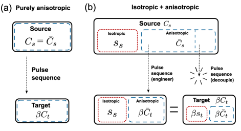
Figure 1: Schematic diagram of interaction engineering. Black solid, red dotted, and blue dashed lines indicate full interactions, isotropic components and anisotropic components, respectively. Dotted arrows represent applications of dynamical decoupling sequence. (a) When both source and target interactions are purely anisotropic ($s_{s}=s_{t}=0$), one directly maps interactions. (b) For interactions with both isotropic and anisotropic components, one engineers only the anisotropic component and matches the relative strength by canceling some fraction.

Let us begin by rewriting $h_{0}$ and $h_{f}$ in their corresponding $C$ matrices $C_{0}$ and $C_{f}$. We denote the strengths of their isotropic components as $s_{0}=\textrm{tr}\left[C_{0}\right]$ and $s_{f}=\textrm{tr}\left[C_{f}\right]$. As previously discussed, if only one of their $C$ is traceless, $h_{0}$ cannot be mapped to $h_{f}$ since the isotropic components can never be decoupled by any pulse sequence. We will now divide our analysis into two cases: (i) $s_{0}=s_{f}=0$ and (ii) $s_{0},s_{f}\neq 0$ (Fig. 1).

Case (i) [Fig. 1(a)]: Our strategy is to cancel the portion of the interaction that is orthogonal to $C_{f}$ while maximizing the strength of the remaining piece. To illustrate this idea more clearly, we introduce a vector representation of interactions

$$\left(\vec{w}\right)_{a}\equiv\textrm{tr}\left[C\eta_{a}\right]/2,$$ (13)

using a matrix basis $\{\eta_{a}\}$ of dimension $m=d^{2}-1$. In this representation, Eq. (8) becomes $\vec{w}_{\textrm{eff}}=\sum_{i}\alpha_{i}M^{i}\vec{w}$ with $M^{i}_{ab}\equiv\frac{1}{2}\textrm{tr}\left[\eta_{a}\left(O^{i}\right)^{T}\eta_{b}O^{i}\right]$. Our objective is to maximize $\vec{w}_{\textrm{eff}}\cdot\vec{w}_{f}$ while satisfying $\vec{w}_{\textrm{eff}}\cdot P_{\perp}=0$, where $\vec{w}_{q}$ ($q\in\{0,f\}$) is the vector representation of $C_{q}$ and $P_{\perp}$ is the projector on to a space that is orthogonal to $\vec{w}_{f}$, i.e., $(P_{\perp})_{ab}=\delta_{ab}-(\vec{w}_{f})_{a}(\vec{w}_{f})_{b}/|\vec{w}_{f}|^{2}$. Interestingly, this task can naturally be cast into the canonical form of Linear Programming, i.e. maximize $\sum_{i}\alpha_{i}\vec{w}_{f}\cdot M^{i}\vec{w}_{0}$ with respect to $\{\alpha_{i}\}$ under constraints $\sum\alpha_{i}P_{\perp}M^{i}\vec{w}_{0}=0$, $\sum\alpha_{i}=1$, and $\alpha_{i}\geq 0$ Bertsimas et al. (1997).

Case (ii) [Fig. 1(b)]: In this case, the contributions from the isotropic components cannot be ignored, and they fix the rescaling parameter, $\beta=s_{0}/s_{1}$. Thus, one has to not only engineer the “shape” of the anisotropic interaction but also adjust its strength to match with the fixed $\beta$. Now our strategy is to decompose the given interaction into three pieces: an isotropic part, a fraction of the anisotropic part to be modified, and the remaining portion to be cancelled. To this end, one is searching for two pulse sequences, $\mathcal{P}_{1}=(\{\tau^{1}_{i}\},\{u^{1}_{i}\})$, which maps $\bar{C}_{0}\mapsto\beta^{*}\bar{C}_{f}$ and $\mathcal{P}_{2}=(\{\tau^{2}_{i}\},\{u^{2}_{i}\})$, which cancels $\bar{C}_{0}\mapsto 0$. Here, $\bar{C}_{q}$ ($q\in\{0,f\}$) is the anisotropic component of $C_{q}$ and $\beta^{*}$ is the maximum possible strength. As before, one can use linear programming to efficiently find these sequences. If both maps are possible and the engineered interaction strength is sufficiently strong $\beta^{*}\geq\beta$, one can concatenate two sequences to form $\mathcal{P}_{3}=(\{(\beta/\beta^{*})\tau^{1}_{i},(1-\beta/\beta^{*})\tau^{2}_{i}\},\{u^{1}_{i},u^{2}_{i}\})$, which maps $C_{0}\mapsto\beta C_{f}$.

Decoupling spin-1 dipolar interactions.—We now turn to two examples. First, we present a 6-pulse sequence that decouples effective dipole-dipole interactions in an ensemble of spin-1 particles (states $\{\left|\pm 1\right>,\left|0\right>\}$) with anharmonic level spacings Kucsko et al. (2016),

$$H_{d}=\sum_{ij}J_{ij} \left[\sum_{a=1}^{2}(X_{a,i}X_{a,j}+Y_{a,i}Y_{a,j})\right.$$ (14)

$$-\left.(Z_{1,i}+Z_{2,i})(Z_{1,j}+Z_{2,j})\right],$$ (15)

where $J_{ij}$ is the interaction strength, while $X_{a,i}$, $Y_{a,i}$, and $Z_{a,i}$ with $a\in\{1,2\}$ are generalized Pauli operators for spin transitions between $\left|0\right>\leftrightarrow\left|+1\right>$ and $\left|0\right>\leftrightarrow\left|-1\right>$, respectively [see Fig. 2(a)]. Such a Hamiltonian is ubiquitous in quantum optical systems and arises in the context of ultracold polar molecules, NV centers, and quadrupolar nuclear spins Yan et al. (2013); Lovchinsky et al. (2017); Choi et al. (2017a). While the solution for the analogous question in dipolar spin-1/2 systems has been known for a half-century (e.g. WAHUHA), the spin-1 problem remains an open question.

Motivated by typical experimental constraints, we assume that the available manipulations are limited to a set of composite pulses constructed from up to four $\pm\pi$ or $\pm\frac{\pi}{2}$-pulses between any of the three transitions with two different phases [Fig. 2(a)]. Using a simple linear programming algorithm, we find an explicit decoupling sequence using only $6$ pulses $\{P_{1},\dots P_{6}\}$ with equal time durations $\tau_{i}=T/6$ as depicted in Fig. 2(b). More detailed explicit expressions for these pulses are provided in Supplementary Material sup . In order to test our sequence, we simulate the dynamics of $N=6$ spin-1 particles with random interaction strengths $J_{ij}\in[-J,J]$ between every pair. We compute the Floquet unitary $U_{T}\equiv P_{6}e^{-iH_{d}T/6}P_{5}\dots P_{1}e^{-iH_{d}T/6}$ and generate stroboscopic time evolution via $(U_{T})^{n}$ with $n\in\mathbb{Z}$. To benchmark the performance of our decoupling sequence, we introduce the fidelity $\mathcal{F}(nT)\equiv|\textrm{tr}\left((U_{T})^{n}\right)/D|^{2}$, where $D=3^{N}$ is the dimension of the Hilbert space. Since $\mathcal{F}(t)=1$ if and only if the evolution corresponds to the identity unitary, the decay of $\mathcal{F}$ serves as a conservative measure of the performance of our interaction decoupling sequence.

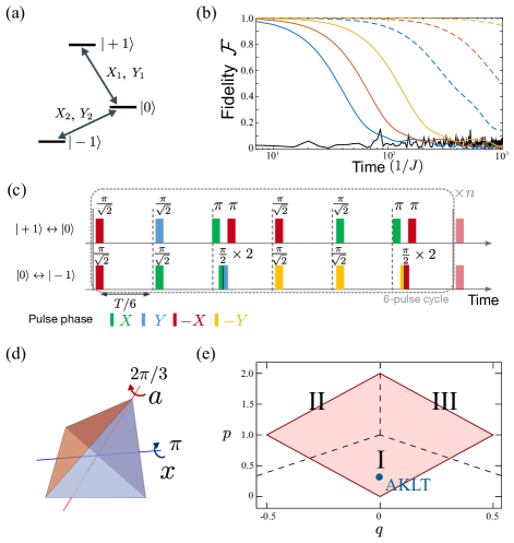
Figure 2: (a) Level diagram for an anharmonic three level system. (b) Decoupling sequence for spin-1 dipolar interactions. Pulse durations are indicated by rotation angles, and phase choices are color-coded. (c) Numerical simulations of decoupling dipolar interactions among $N=6$ spin-1 particles. Black solid line indicates $\mathcal{F}(t)$ in the absence of pulse sequence. Blue, red, and yellow solid lines correspond to $\mathcal{F}(t)$ under a decoupling sequence with $1/JT=3,5,10$, respectively. Dashed lines are for symmetrized sequences. (d) Two generators $\{a,x\}$ of the symmetry group $A_{4}$. (e) Phase diagram. Three SPT phases (I, II, and III) are distinguished by the transformation of ground state wavefunctions under the action of $a\in A_{4}$. The colored area indicates the domain of $(p,q)$ that can be engineered from Ising interactions. Blue dot indicates the AKLT point $(p,q)=(1/3,0)$.

Figure 2(c) depicts $\mathcal{F}(t)$ for various values of $T$, demonstrating that the evolution remains trivial up to $\sim 10/J$ for $JT<1$ (colored solid lines). Once a given decoupling sequence is found, one can always symmetrize it to further suppress the leading order correction in Magnus expansion sup . In our case, such a sequence involves 10 pulses within the period $2T$. Shown as dashed lines in Fig. 2 (c), the symmetrized sequence significantly suppresses the interaction for timescales up to $\sim 100/J$. More generally, it has been rigorously shown that effective dynamics is well captured by low order Magnus expansion up to a long time that scales exponentially in $1/T$ Abanin et al. (2017, 2015); Mori et al. (2016); Kuwahara et al. (2016).

Engineering SPT Hamiltonians.—As a second example, we show that a spin-1 chain with nearest neighbor Ising interactions can be directly mapped to a family of SPT Hamiltonians sup . More specifically, given a basic Ising interaction $H_{I}=\sum_{i}S_{i}^{z}S_{i+1}^{z}$, one can engineer a two-parameter family of Hamiltonians $H(p,q)=H_{1}+pH_{2}+qH_{3}$ with

$$H_{1} =\sum_{i}\vec{S}_{i}\cdot\vec{S}_{i+1},\;\;H_{2}=\sum_{i}(\vec{S}_{i}\cdot\vec{S}_{i+1})^{2},$$

$$H_{3} =\sum_{i}\sum_{(a,b,c)\in S_{3}}(S_{i}^{a}S_{i}^{b}S_{i+1}^{c}+S_{i}^{a}S_{i+1}^{b}S_{i+1}^{c}),$$

where $p,q\in\mathbb{R}$, $\vec{S}_{i}=(S^{x}_{i},S^{y}_{i},S^{z}_{i})$ is the spin-1 vector operator, and $\sum_{(a,b,c)\in S_{3}}$ indicates the summation over all permutations of $(x,y,z)$. The symmetries of the Hamiltonian include lattice translation, the bond-centered inversion, and a global internal symmetry $A_{4}$, which is the symmetry group of a tetrahedron [see Fig 2(d)]. All possible SPT phases protected by these symmetries are explicitly enumerated in Ref. Prakash et al. (2016).

When $p=1/3$ and $q=0$, the Hamiltonian reduces to celebrated Affleck-Kennedy-Lieb-Tasaki (AKLT) model, whose ground state is exactly solvable and exhibits non-trivial topological edge degrees of freedom Affleck et al. (1987). As $(p,q)$ deviates from this solvable point, phase transitions arise among three distinct regions, I, II, and III, indicated in the numerically obtained phase diagram in Fig. 2(e) sup . The ground states in the three phases respect all the symmetries while they are distinguished by the complex $U(1)$ phase that the state picks upon a $120^{\circ}$ rotation $a\in A_{4}$ of underlying spins sup . Using our algorithm, we find that $H(p,q)$ with $2|q|\leq p\leq 2-2|q|$ can be engineered from $H_{I}$ [colored area in Fig. 2(e)]. The relative strength of $H(p,q)$ is set to $1/(3+p)$ by isotropic components, and the range of $(p,q)$ is limited by the maximum possible strength of the engineered anisotropic components sup . Interestingly, the triple point at $(p,q)=(1,0)$ corresponds to purely isotropic interactions, where the Hamiltonian possesses a larger symmetry group (i.e. full $SU(d)$).

Discussions.— We now consider the dominant operational imperfections which may arise during the proposed Hamiltonian engineering protocol. First, our periodic driving pulses may cause heating in the many-body system, eventually leading to a featureless infinite temperature state D’Alessio and Rigol (2014); Lazarides et al. (2014); Ponte et al. (2015). Such effects are discussed in Ref. Abanin et al. (2017); Mori et al. (2016); Abanin et al. (2015); Kuwahara et al. (2016), and it has been shown that such energy absorption becomes relevant only after exponentially long times $t^{*}\sim\exp{[O(1/\bar{J}T)]}$, where $\bar{J}\equiv\max_{i,j}J_{ij}||h_{ij}||$. A second natural concern is that our method is based upon engineering the leading order Magnus Hamiltonian $H_{\textrm{eff}}^{(0)}$, which provides only an approximate description of the full many-body dynamics. However, for gapped Hamiltonians, one expects that higher order terms in the Magnus expansion are strongly suppressed so long as $\bar{J}T\ll 1$, implying that the phase should remain stable. Finally, adiabatic change of parameters can be used to prepare the system in a low-entropy state close to the ground state of the effective Hamiltonian.

Interestingly, the decoupling of interactions may result in dynamical quantum phase transitions for isolated, weakly disordered systems Choi et al. (2017b). In such cases, the interplay of weak disorder, suppressed interactions, and an exponentially slow heating rate can lead to many-body localization, where initial state memories survive for extremely long times. Harnessing these effects may enable the coherent manipulation and storage of quantum information in an interacting many-body system Choi et al. (2015); Yao et al. (2015).