Grouped Convolutional Neural Networks for Multivariate Time Series

Abstract

Analyzing multivariate time series data is important for many applications such as automated control, fault diagnosis and anomaly detection. One of the key challenges is to learn latent features automatically from dynamically changing multivariate input. In visual recognition tasks, convolutional neural networks (CNNs) have been successful to learn generalized feature extractors with shared parameters over the spatial domain. However, when high-dimensional multivariate time series is given, designing an appropriate CNN model structure becomes challenging because the kernels may need to be extended through the full dimension of the input volume. To address this issue, we present two structure learning algorithms for deep CNN models. Our algorithms exploit the covariance structure over multiple time series to partition input volume into groups. The first algorithm learns the group CNN structures explicitly by clustering individual input sequences. The second algorithm learns the group CNN structures implicitly from the error backpropagation. In experiments with two real-world datasets, we demonstrate that our group CNNs outperform existing CNN based regression methods.

1 Introduction

Advances in computing technology has made many complicated systems such as automobile, avionics, and industrial control systems more sophisticated and sensitive. Analyzing multiple variables that compose such systems accurately is therefore becoming more important for many applications such as automated control, fault diagnosis, and anomaly detection.

In complex systems, one of the key requirements is to maintain integrity of the sensor data so that it can be monitored and analyzed in a trusted manner. Previously, sensor integrity has been analyzed by feedback controls (Mo & Sinopoli, 2015; Pajic et al., ) and nonparametric Bayesian methods (Krause et al., 2008). However, regression models based on control theory and nonparametric Bayesian are highly sensitive to the model parameters. Thus, finding the best model parameter for the regression models is challenging with high-dimensional multivariate sequences.

Artificial neural network models also have been used to handle multivariate time series data. Autoencoders (Bourlard & Kamp, 1988; Zemel, 1994) train model parameters in an unsupervised manner by specifying the same input and output values. Recurrent neural networks (RNN) (Rumelhart et al., ) and long-short term memory (LSTM) (Hochreiter & Schmidhuber, 1997) represent changes of time series data by learning recurrent transition function between time steps. Unfortunately, existing neural network models for time series data assume fully connected networks among time series under the Markov assumption. Thus, such models are often not precise enough to address high-dimensional multivariate regression problems.

To address this issue, we present two structure learning algorithms for deep convolutional neural networks (CNNs). Both of our algorithms partition input volume into groups by exploiting the covariance structure for multiple time series so that the input CNN kernels process only one of the grouped time series. Due to this partitioning of the input time series, we can avoid the CNN kernels being extended through the full dimension. In this reason, we denote the CNN models as Group CNN (G-CNN) which can exploit latent features from multiple time-series more efficiently by utilizing structural covariance of the input variables.

The first structure learning algorithm learns the CNN structure explicitly by clustering input sequences with spectral clustering (Luxburg, 2007). The second algorithm learns the CNN structures implicitly with the error backpropagation which will be explained in Section 3.2.

Our model design principle is to reduce model parameters by sharing parameters when necessary. In multivariate time series regression tasks, our hypotheses on the parameter sharing scheme (or parameter tying) are as follow: (1) convolutions on a group of correlated signals are more robust to signal noises; and (2) convolutions operators on groups of signals are more feasible to learn when a large number of time series is given. In experiments, we show that G-CNN make the better predictive performance on challenging regression tasks compared to the existing CNN based regression models.

2 Background

2.1 Convolutional Neural Network

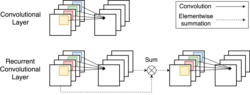
Figure 1: Building blocks of CNN and RCNN.

A convolutional neural network (CNN) is a multi-layer artificial neural network that has been successful recognizing visual patterns. The most common architecture of the CNNs is a stack of three types of multiple layers: convolutional layer, sub-sampling layer, and fully-connected layer. Conventionally, A CNN consists of alternate layers of convolutional layers and sub-sampling layers on the bottom and several fully-connected layers following them.

First, an unit of a convolutional layer receives inputs from a set of neighboring nodes of the previous layer similarly with animal visual cortex cell. The local weights of convolutional layers are shared with the nodes in the same layer. Such local computations in the layer reduce the memory burden and improve the classification performance.

None-linear down-sapling layer, which is the second type of CNN layers, is another important characteristic of CNNs. The idea of local sub-sampling is that once a feature has been detected, its location itself is not as important as its relative location with other features. By reducing the dimensionality, it reduces the local sensitivity of the network and computational complexity (LeCun & Bengio, 1995; LeCun et al., 1998).

The last type of the layers is the fully-connected layer. It computes a full matrix calculation with all activations and nodes same as regular neural networks. After convolutional layers and sub-sampling layers extract features, fully-connected layers implements reasoning and gives the actual output. Then the model is trained in the way minimizing the error between the actual output of the model and the target output values by backpropagation method.

CNN has been very effective for solving many computer vision problems such as classification (LeCun et al., 1998; Krizhevsky et al., 2012), object detection and semantic segmentation (Ren et al., 2015; Long et al., 2015). It has been also applied to other problems such as natural language processing (Kalchbrenner et al., 2014; Collobert & Weston, 2008). Recently, variants of CNN are applied to analyzing various kinds of time-series such as sensor values and EEG (electroencephalogram) signals (Yang et al., 2015; Ordóñez & Roggen, 2016).

2.2 Recurrent Convolutional Neural Network (RCNN)

Recurrent Convolutional Neural Network (RCNN) is a type of CNN with its convolutional layers being replaced with recurrent convolutional layers. It improves the expressive power of the convolutional layer by exploiting multiple convolutional layers that share the parameters. RCNN has been applied to not only the image processing problem (Liang & Hu, 2015; Pinheiro & Collobert, 2014) but also other tasks that require temporal analysis (Lai et al., 2015). RCNN can effectively extract invariant features in the temporal domain regarding the time-series data as a 2-dimensional data with one of the dimensions is one. with one of the dimensions is 1, RCNN can effectively extract invariant features in the temporal domain.

2.2.1 Recurrent Convolutional Layer

Recurrent Convolutional Layer (RCL), which is the most representative building block of an RCNN, is the composition of $l$ intermediate convolutional layers that shares the same parameters. The first convolutional layer of an RCL carries the convolution on the input x, resulting in the output $\sigma(W*\textbf{x})$ where $W$ is the convolutional filter, * is a convolution operator, and $\sigma(\cdot)$ is an activation function. Then the next convolutional layer recursively processes the summation of the original input and the output of the previous layer, $\textbf{x}+\sigma(W*\textbf{x})$, as an input. After some iterations of this process, an RCL gives the result of the final intermediate convolutional layer as its output.

During the error backpropagation, the parameters are updated $l$ times. In each update, the parameters are changed to fix the error made by itself from the previous layer.

RCL can also be regarded as a skip-layer connection (He et al., 2015; Intrator & Intrator, 2001). Skip-layer connection represents connecting layers skipping intermediate layers as in Figure 1’s RCL. The main motivation is that the deeper networks show a better performance in many cases but they are also harder to train in actual applications due to vanishing gradients and degradation problem (Bengio et al., 1994; Glorot & Bengio, 2010).

(He et al., 2015) designed such layers with skip-layer connection, named as residual learning. The idea was that if one can hypothesizes that multiple nonlinear layers can estimate an underlying mapping $H(x)$, it is equivalent to estimating an residual function $F(x)\mathrel{\mathop{\mathchar 58\relax}}=H(x)-x$. If the residual $F(x)$ is approximately a zero mapping, $H(x)$ is an optimal identity mapping.

2.3 Spectral Clustering

The goal of clustering data points $\mathbf{x}_{1},...,\mathbf{x}_{N}$ is to partition the data points into some groups such that the points in the same group are similar and points in different groups are dissimilar in a certain similarity measure $s_{ij}$ between $x_{i}$ and $x_{j}$. Spectral clustering is the clustering method that solves this problem from the graph-cut point of view.

From the graph-cut point of view, data points are represented as a similarity graph $G=(V,E)$. Let $G$ be a weighted undirected graph with the vertex set $V=\{v_{1},...,v_{N}\}$ where each vertex $v_{i}$ represents a data point $x_{i}$ and the weighted adjacency matrix $W=\{w_{ij}|i,j=1,...,N\}$ where $w_{ij}$ represents the similarity $s_{ij}$. Let the degree of a vertex $v_{i}\in V$ be $d_{i}=\sum^{n}_{j=1}w_{ij}$ and define a degree matrix $D$ as the diagonal matrix with the degrees $d_{1},...,d_{N}$ on the diagonal.

Then, clustering can be reformulated to find a partition of the graph such that the edges between different groups have very low weights and the edges within a group have high weights.

One of the most intuitive way to solve this problem is to solve the min-cut problem (Shi & Malik, 2000). Min-cut problem is to choose a partition $A_{1},...,A_{K}$ for a given number $K$ that minimizes the equation (2.3.1) given as:

$$\mbox{cut}(A_{1},...,A_{K}) \mathrel{\mathop{\mathchar 58\relax}}=\frac{1}{2}\sum_{i=1}^{K}\mbox{link}(A_{i},\bar{A}_{i})$$ (2.3.1)

$$\textnormal{s.t. }\mbox{link}(A,B) \mathrel{\mathop{\mathchar 58\relax}}=\sum_{i\in A,j\in B}w_{ij}\textnormal{ for disjoint }A,B\subset A.$$ (2.3.2)

Here, 1/2 is introduce for normalizing as otherwise each edge will be counted twice. The algorithm of (Shi & Malik, 2000) explicitly requests the sets be large enough where the size of a subset $A\subset V$ is measured by:

$$\mbox{vol}(A)\mathrel{\mathop{\mathchar 58\relax}}=\sum_{i\in A}d_{i}$$ (2.3.3)

Then, find the following normalized cut, Ncut:

$$\mbox{Ncut}(A_{1},...,A_{K})\mathrel{\mathop{\mathchar 58\relax}}=\frac{1}{2}\sum_{i=1}^{K}\frac{\mbox{link}(A_{i},\bar{A}_{i})}{\mbox{vol}(A_{i})}$$ (2.3.4)

The denominator of the Ncut tries to balance the size of the clusters and the numerator finds the minimum cut of the given graph. Then to find the partition $A_{1},...,A_{K}$ is same as to solve the following optimization problem:

$$\min_{H\in\mathbb{R}^{NxK}}trace(H^{T}LH)$$ (2.3.5)

$$s.t.\hskip 30.00005pt H_{ij}\mathrel{\mathop{\mathchar 58\relax}}=\begin{cases}\frac{1}{\sqrt{vol(V_{j})}},v_{i}\in V_{j}\\ 0,otherwise\end{cases}$$ (2.3.6)

$$L\mathrel{\mathop{\mathchar 58\relax}}=D-W$$ (2.3.7)

As $h^{T}_{i}Lh_{i}{=}\mbox{cut}(A_{i},\bar{A}_{i})/\mbox{vol}(A_{i})$, $H^{T}H{=}I$, and $h_{i}^{T}Dh_{i}{=}1$ where the indicator vector $h_{j}$ is the j-th column of the matrix H.

Unfortunately, introducing the additional term to the min-cut problem has proven to make the problem NP-hard (Wagner & Wagner, 1993) so (Luxburg, 2007; Bach & Jordan, 2004) solves the relaxed problem, which gives the solution H that consists of the eigenvectors corresponding to the K smallest eigenvalues of the matrix $L_{rw}\mathrel{\mathop{\mathchar 58\relax}}=D^{-1}L$ or the K smallest generalized eigenvectors of $Lu=\lambda Du$.

Given an $N$x$N$ similarity matrix, the spectral clustering algorithm runs eigenvalue decomposition (EVD) on the graph Laplacian matrix and the eigenvectors corresponding to the K smallest eigenvalues are clustered by a clustering algorithm representing the graph vertices. The K eigenvectors are also the eigenvectors of the similarity matrix whereas corresponding K largest eigenvalues, which can be considered as an encoding of the graph similarity matrix.

3 Grouped Time Series

In this section, we present two algorithms build group CNN structure. The first method builds the group structure explicitly from Spectral clustering. The second method build the group structure through the error backpropagation.

3.1 Learning the Structure by Spectral Clustering

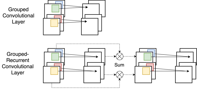
Figure 2: Grouped layers for CNN and RCNN.

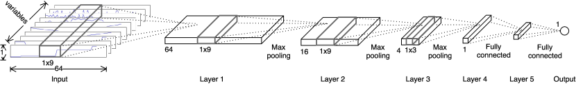
(a) Convolutional Neural Network (CNN).

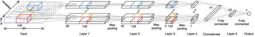
(b) CNN with grouped convolutional layers.

Figure 3: Comparison of the general CNN model and CNN with grouped layers.

Our group CNN structure receives both the input variables $\mathbf{X}=[\mathbf{x}_{1},...,\mathbf{x}_{N}]$ and their cluster information $C=[c_{1},...,c_{N}]$ where $c_{i}$ represents the membership of the variable $x_{i}$. Unlike usual convolutional layers, the grouped convolutional layers divide the input volume based on the cluster membership $c_{i}$ and performs the convolution operations over the input variables that belong to the same cluster as described in the Figure 2. Formally, the k-th group of the layer H is defined as:

$$H^{k}=\sigma\big{(}\sum_{i}W^{k}\cdot\mathbf{x}_{i}+b^{k}\big{)}$$ (3.1.1)

where $(\cdot)$ is the convolution operation, $i\in\{j|j\in\{1,...,N\},c_{j}=k\}$, $W^{k}$ is the weight matrix, and $b_{k}$ is the bias vector of the k-th group.

As in the CNN models, the input variables $X$ are processed throughout multiple grouped convolutional layers and sub-sampling layers, flattened into one-dimensional layer followed by fully-connected layers, and produces the output $\mathbf{y}=\{y_{1},...,y_{P}\}$ (Figure 3).

Given the target output $\mathbf{t}=\{t_{1},...,t_{P}\}$, we can also train this model using gradient descent solving the optimization problem:

$$\min_{\theta}\sum_{i=1}^{p}(y_{i}-t_{i})^{2}$$ (3.1.2)

with respect to the trainable parameter $\theta=\{W,b\}$. The error is backpropagated to each group separately, training the CNN structure explicitly.

This model requires significantly less number of parameters compared to the vanilla CNN model. For example, to process 100 input variables producing 100 output channel, existing CNN model needs 100 kernels of size (width, height, 100). However, if the input variables consist of 5 clusters, each with 20 variables, it requires 5x20 kernels of size (width, height, 20), which is 5 times less than the vanilla model. It could make the CNN model more compact by eliminating redundant parameters.

3.2 Neural Networks with Clustering Coefficient

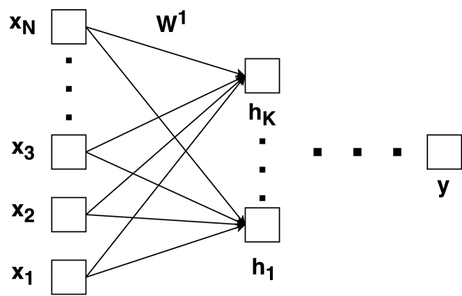
Figure 4: Example of a neural network that receives grouped variables.

Assuming that the input time series are correlated with each other, we group those variables explicitly to make use of such correlations as CNN utilizes local connectivity of an image. It can be considered to find the local connectivity and correlations within channels of CNN.

Given an input data $X$ which consists of N variables where each variables are $D$ dimensional real valued vectors, i.e. $X=[\mathbf{x}_{1},...,\mathbf{x}_{N}]$, we wish to group these variables into K clusters introducing a matrix $U=[u_{i,j};i\in\{1,...,N\},j\in\{1,...,K\}]$ where $u_{i,j}\in[0,1],\sum_{j}^{K}u_{i,j}=1$ whose element $u_{i,j}$ is the clustering coefficient which represents the portion of the $j$-th cluster takes for the variable $\mathbf{x}_{i}$ as in multinomial distribution. In this paper, we use boldface letters to represent D-dimensional real valued column vectors.Then, $\mathbf{h}_{j}$, the node that represents the j-th cluster is defined as :

$$\mathbf{h}_{j}=\sigma(\sum_{i}^{N}u_{i,j}\mathbf{x}_{i}^{T}\cdot\mathbf{W}^{1}_{i,j}+\mathbf{b}^{1}_{j})$$ (3.2.1)

where $\mathbf{W}^{1}_{i,j}$ is the i-th row’s j-th column of the weight matrix $W^{1}$ of size $N$x$K$, $\mathbf{b}^{1}_{j}$ is the bias, and $\sigma(\cdot)$ is the activation function. By multiplying $u_{i,j}$, variables can proportionally participate to each cluster.

Suppose that an example of two layered neural network is given as shown in the Figure 4. The output node $\mathbf{y}$ is also defined as :

$$\mathbf{y}=\sigma(\sum_{j}^{K}\mathbf{h}_{j}^{T}\cdot\mathbf{W}^{2}_{j,1}+\mathbf{b}^{2}_{1}).$$ (3.2.2)

Given the true target value $\mathbf{t}$, this network can be trained by gradient descent method solving the below optimization problem:

$$\min_{W,U,B} Err,$$ (3.2.3)

$$Err\mathrel{\mathop{\mathchar 58\relax}}= \frac{1}{2}(\mathbf{y}-\mathbf{t})^{2}$$ (3.2.4)

Assuming linear activation function, gradient of the $Err$ with respect to $u_{i,j}$ is :

$$\frac{\partial Err}{\partial u_{i,j}} =\frac{\partial Err}{\partial\mathbf{y}}\frac{\partial\mathbf{y}}{\partial u_{i,j}}$$

$$=\frac{\partial Err}{\partial\mathbf{y}}\frac{\partial\mathbf{y}}{\partial\mathbf{h}_{j}}\frac{\partial\mathbf{h}_{j}}{\partial\mathbf{u}_{i,j}}$$

$$=\frac{\partial Err}{\partial\mathbf{y}}(\frac{\partial\mathbf{h}^{T}_{j}}{\partial u_{i,j}}+\sum_{j^{\prime}}^{K}\mathbf{I}\{j^{\prime}\neq{j}\}\frac{\partial\mathbf{h}^{T}_{j^{\prime}}}{\partial u_{i,j^{\prime}}}\frac{\partial u_{i,j^{\prime}}}{\partial u_{i,j}})\frac{\partial\mathbf{h}_{j}}{\partial\mathbf{u}_{i,j}}$$

$$=(\mathbf{y}-\mathbf{t})(\mathbf{K}\mathbf{x}^{T}_{i}\cdot\mathbf{W}^{1}_{i,j}-\sum_{j}^{K}\mathbf{x}^{T}_{i}\cdot\mathbf{W}^{1}_{i,j})(\mathbf{x}^{T}_{i}\cdot\mathbf{W}^{1}_{i,j})$$ (3.2.5)

where $j^{\prime}$ is the cluster out of the j-th cluster and $\mathbf{I}$ is an indicator function. Intuitively, the parameter update $u_{i,j}$ includes (K times of loss from the j-th cluster - loss from all clusters ; $\mathbf{K}x^{T}_{i}\cdot\mathbf{W}^{1}_{i,j}-\sum_{j}^{K}\mathbf{x}^{T}_{i}\cdot\mathbf{W}^{1}_{i,j})$, $u_{i,j}$ value that gives smaller loss increase finding the optimal values while minimizing the error by the gradient descent method.

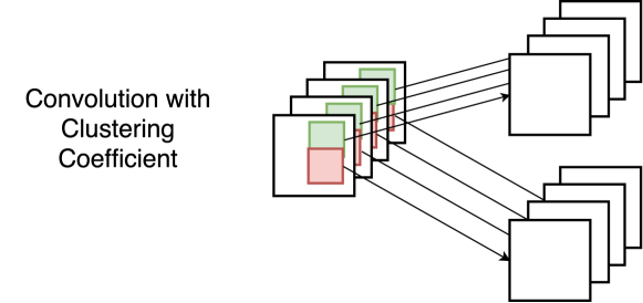
Figure 5: Convolutional layer with clustering coefficient.

To implement the clustering coefficient to out model, we added a new layer which works as the Figure 5 on the bottom of the model, before the layer 1 of the Figure  3 (b). This layer receives $N$ input variables and computes channel-wise convolution throughout the variables using the same weight and bias in the group (group parameter sharing). This channel-wise convolution is repeated for K groups with different parameters for each groups. Therefore, the i-th channel of the k-th group is defined as:

$$h^{K}_{i}=\sigma(u_{i,k}W^{k}\cdot\mathbf{x}_{i}+b^{k})$$ (3.2.6)

Then the output is processed by the same process with the model from the Section 3.1 with explicit clustering.

4 Related Work

Recently, deep learning methods are making good results in solving a variety of problems such as visual pattern recognition, signal processing, and others. Consequently there has been researches for applying those methods to analyzing complex multivariate systems.

Neural networks that are composed of fully-connected layers only are not appropriate for handling sequential data since they need to process the whole sequence of input. More specifically, such networks are too inefficient in terms of both memory usage and learning efficiency.

One of the popular choices for processing time-series is a recurrent neural network (RNN). An RNN (Williams & Zipser, 1989; Funahashi & Nakamura, 1993) processes sequential data with recurrent connections to represent transition models over time. so that it can store temporal information within the network. RNN models have been successfully used for processing sequential data (Mozer, 1993; Pascanu et al., 2013; Koutnik et al., 2014). (Coulibaly & Baldwin, 2005) used dynamic RNN to forecast nonstationary hydrological time-series and (Malhotra et al., 2015) used stacked LSTM network as a predictor over a number of time steps and detected anomalies that has high prediction error in time series.

Convolutional neural network (CNN) is also commonly used to analyze temporal data.(Abdel-Hamid et al., 2012) used CNN for speech recognition problem and (Zheng et al., 2014) proposed multi-channels deep convolutional neural network for multivariate time series classification.

Recurrent Convolutional Neural Network (RCNN), which can be considered as a variant of a CNN, is recently proposed and shows state-of-the-art performance on classifying multiple time series (Pinheiro & Collobert, 2014; Liang & Hu, 2015; Lai et al., 2015). When a small number of time series is given, multiple signals can be handled individually in a straightforward manner by using polling operators or fully connected linear operators on signals. However, it is not clear how to model the covariance structure of large number of multiple sequences explicitly for deep neural network models.

5 Experimental Results

In experiments, we compare the regression performance of several CNN-based models on two real-world high-dimensional multivariate datasets, groundwater level data and drone flight data. Groundwater data and drone data respectively have 88 and 148 variables.

	Model	Input	Layer 1	Layer 2	Layer 3	Layer 4	Layer 5	Output
	CNN	1x64x87	1x64x500	1x16x500	1x4x500	1x1x500	100	1
	RCNN3	1x64x87	1x64x500	1x16x500	1x4x500	1x1x500	100	1
Water1	CNN & exp	1x64x87	(1x64x100)54	(16x100)5	(4x100)5	(1x100)5	100	1
	RCNN3 & exp	1x64x87	(1x64x100)5	(16x100)5	(4x100)5	(1x100)5	100	1
	CNN & coeff 6	1x64x87	(1x64x100)5	(16x100)5	(4x100)5	(1x100)5	100	1
	RCNN & coeff	1x64x87	(1x64x100)5	(16x100)5	(4x100)5	(1x100)5	100	1
	CNN	1x64x147	1x64x750	1x16x750	1x4x750	1x1x750	200	1
	RCNN3	1x64x147	1x64x750	1x16x750	1x4x750	1x1x750	200	1
Drone2	CNN & exp	1x64x147	(1x64x50)155	(1x16x50)15	(1x4x50)15	(1x1x50)15	200	1
	RCNN3 & exp	1x64x147	(1x64x50)15	(1x16x50)15	(1x4x50)15	(1x1x50)15	200	1
	CNN & coeff 6	1x64x147	(1x64x50)15	(1x16x50)15	(1x4x50)15	(1x1x50)15	200	1
	RCNN & coeff	1x64x147	(1x64x50)15	(1x16x50)15	(1x4x50)15	(1x1x50)15	200	1

¹Groundwater Dataset. ²Drone Dataset. ³Layer 1, Layer 2, Layer 3 are RCLs with iteration 2. ⁴K=5. ⁵K=15.
⁶Models with clustering coefficient has an additional layer (Figure 5) before the Layer 1.

Table 1: Architecture of tested deep CNN models.

5.1 Settings

To evaluate the regression performance, we picked one of the variables, say $x_{p}$, from the dataset randomly and constructed the variable’s values as a target at time t, $y=x_{p}(t)$, by seeing its correlated variables’ values from time $t-T$ to $t$ without including variable, i.e. $X=\cup_{i,i\neq p}[x_{i}(t-T),...,x_{i}(t)]$.

We trained our models with $90\%$ of the whole dataset and tested on the other $10\%$. Then, the regression performance were compared with other regression models: linear regression, ridge regression, CNN and RCNN. The regression performance was measured on the scale of the standardized root mean square error (SRMSE), which is defined as the equation 5.1.1 when $\bar{t}$ is the mean value of the target vector $\mathbf{t}$.

SRMSE $$=\frac{\sqrt{\Sigma_{t=1}^{N}(t_{t}-y_{t})^{2}/N}}{SE}$$ (5.1.1)

$$SE =\sqrt{\frac{1}{N}\sum_{i}(t_{i}-\bar{t})^{2}}$$ (5.1.2)

5.2 Datasets

5.2.1 Groundwater Data

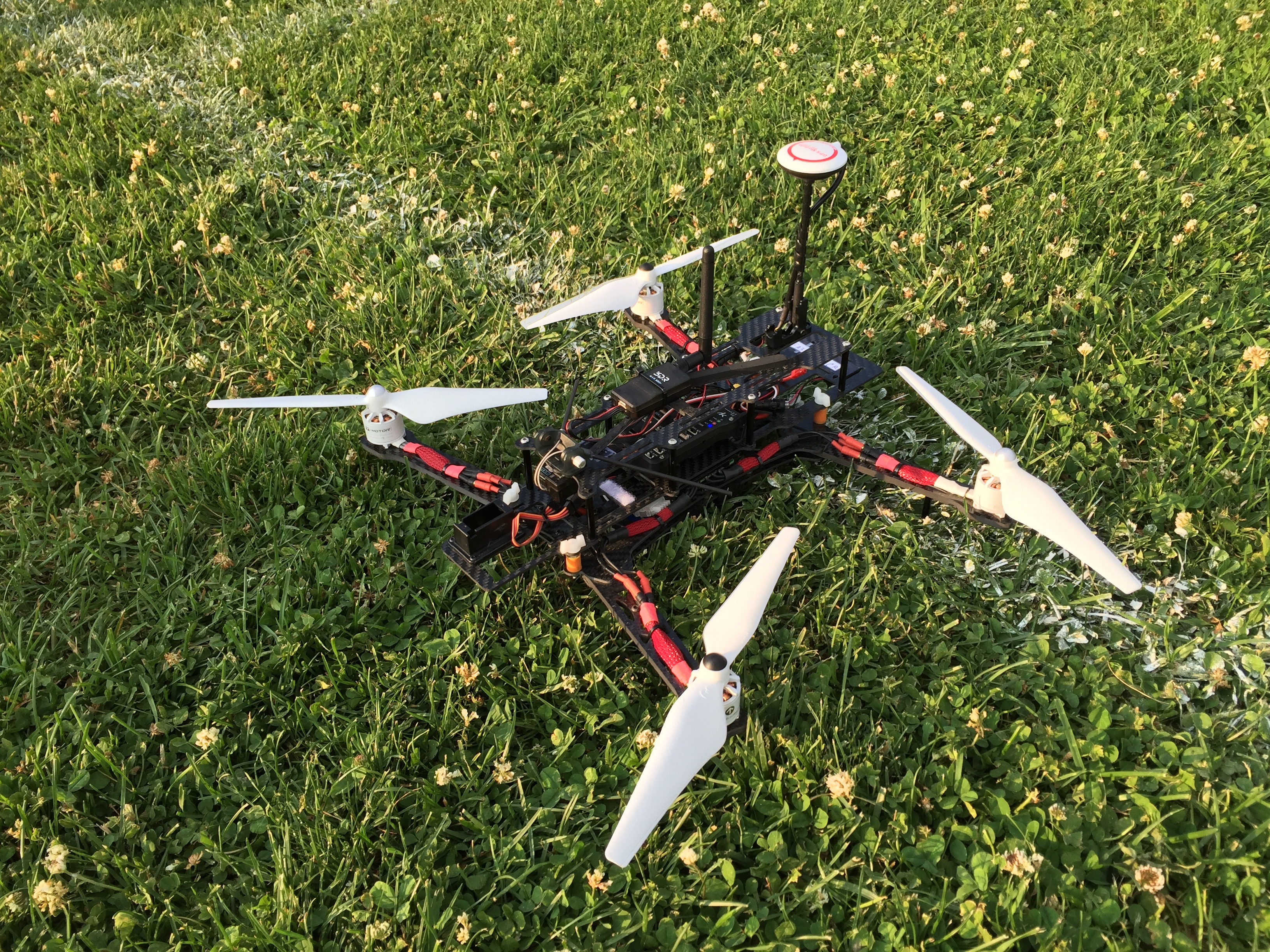
(a) quadcopter used for the test.

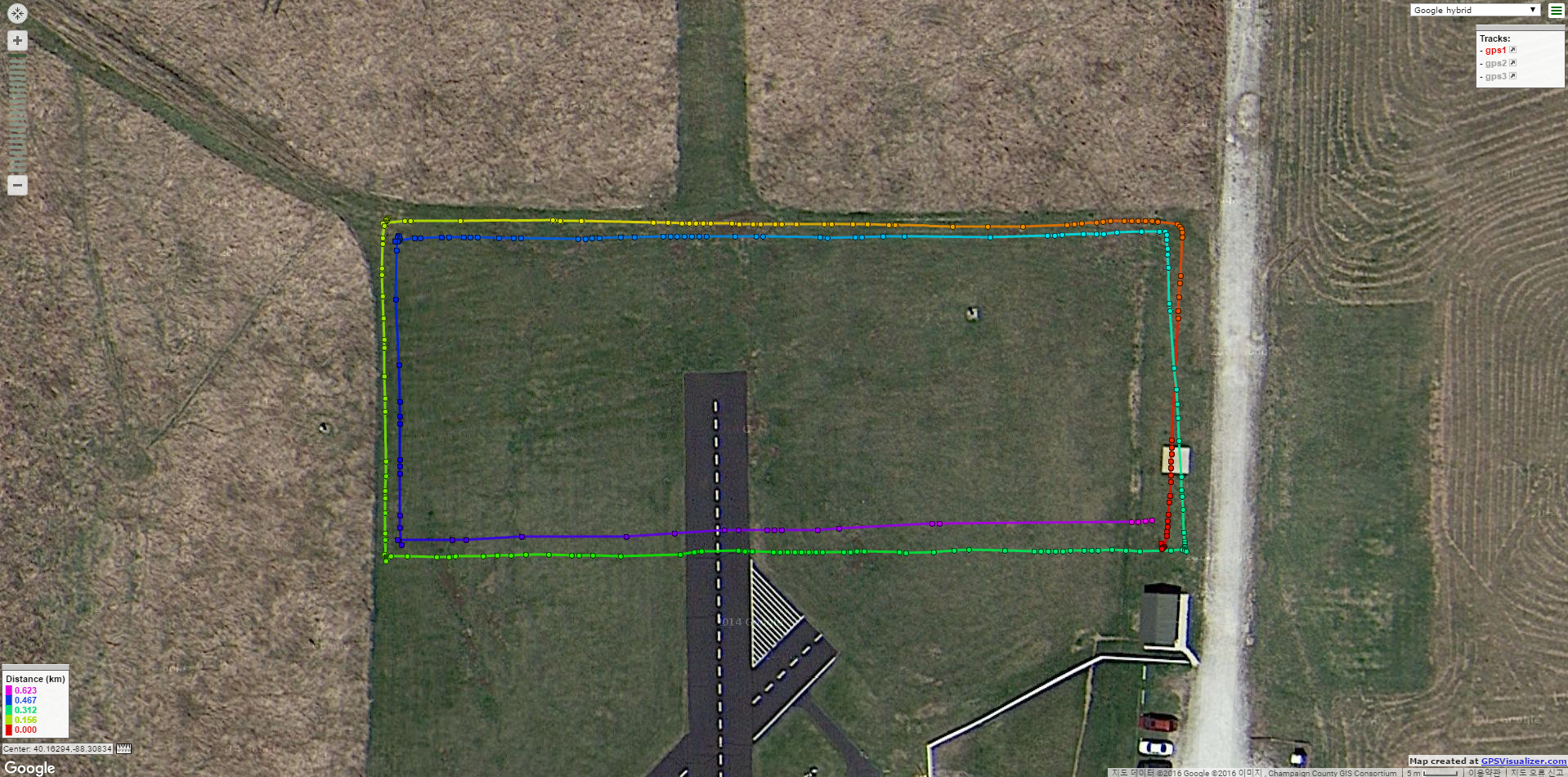
(b) drone’s flight path.

Figure 6: Drone.

We used daily collected groundwater data provided by the United States Geological Survey (USGS). Dataset is composed of various parameters from the US territories and we used depth to water level from the regions other than Hawaii and Alaska. Regions where the data was collected over 28 years (1987-2015) were selected and those that have unrecorded periods longer than two months were excluded. Empty records shorter than two months were filled by interpolation. Final dataset contains records from 88 sites of 10,228 days.

5.2.2 Drone Data

We used a quadcopteras our experimental platform to collect flight sensor data. Quadcopters are aerodynamically unstable and their actuators, i.e., the motors, must be controlled directly by an on-board computer for stable flight. We used the Pixhawk as the autopilot hardware for our quadcopter. It has on-board sensors such as inertial measurement unit (IMU), compass, and barometer. We run the open-source PX4 autopilot software suite on the ARM Cortex M4F processor on the Pixhawk. It combines sensor data and flight commands to compute correct outputs to the motors, which then controls the vehicle’s orientation and position.

We collected flight data of the quadcopter using PX4’s autopilot logging facility. Each flight data is composed of time-stamped sensor and actuator measurements, flight set points (attitude, position), and other auxiliary information (radio input, battery status, etc.). We collected data sets by flying the quadcopter in an autonomous mode, in which it flies along a pre-defined path. We obtained three sets of logs by varying the path as shown in Figure 6. In total, we used 148 sensors of 12,654 time points excluding those that do not show any change during the flight and have missing values.

5.3 Results

We built group CNN and group RCNN using both spectral clustering method (explicit) and the clustering coefficient method (coeff), and compared the performance with corresponding vanilla CNNs and vanilla RCNNs. The deep CNN model architecture are shown in Table 1. All the learning parameters such as the learning rate and weight initialization parameters are matched. Every models were trained for 200 epochs and the best results were chosen.

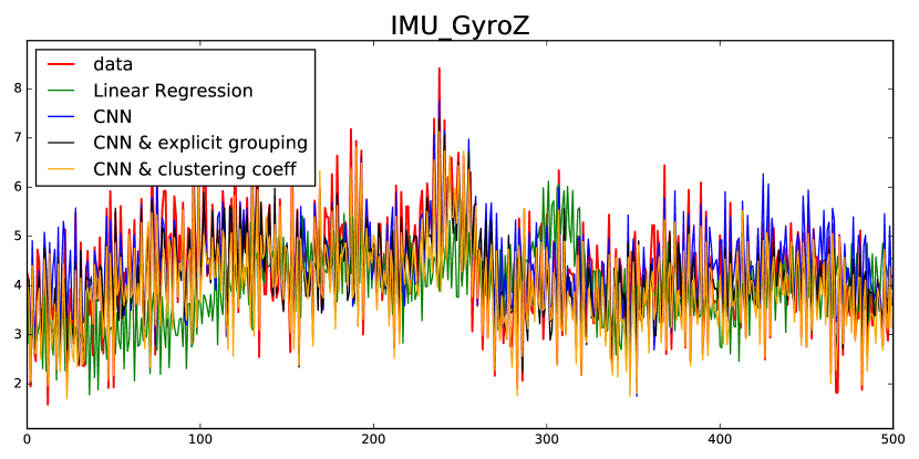
(a) Drone IMU_GyroZ sensor.

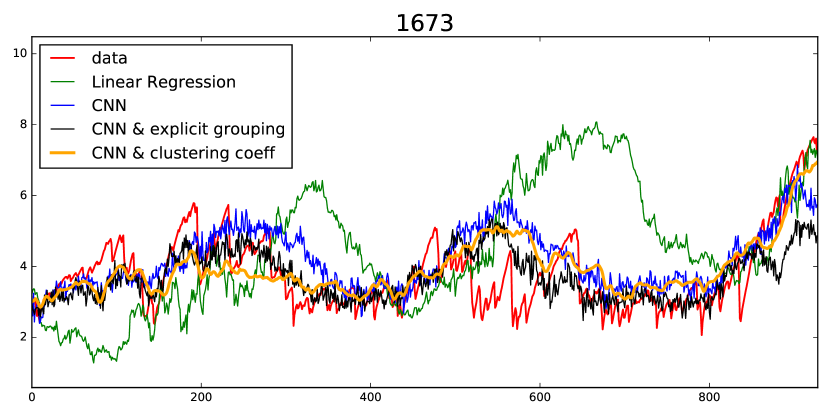
(b) Groundwater site 1673.

Figure 7: Reconstruction examples on the test data.

Experiment results are shown in the following tables, Table 2 and Table 3. In general, our group CNN models outperform in the groundwater dataset. RCNN with clustering coefficient model performs best with 0.754 SRMSE compared to 0.985 of vanilla RCNN model. Our group CNN models also tend to perform better than the vanilla CNN models in the drone flight dataset. RCNN with spectral clustering model performs best with 0.438 SRMSE compared to 0.464 SRMSE of vanilla CNN model. The values predicted by our models are shown in Figure 7.

SRMSE	Mean	STDEV
Linear Regression	$1.298$	$0.469$
Ridge Regression	$1.298$	$0.469$
CNN	$0.999$	$0.340$
RCNN1	$0.985$	$0.408$
CNN & explicit	$0.861$	$0.195$
RCNN1 & explicit	$0.929$	$0.347$
CNN & coeff	$0.783$	$0.254$
RCNN & coeff	$\bf{0.754}$	$0.217$

¹RCNN with three RCLs of iteration 2-2-2.

Table 2: SRMSE of regression on Groundwater data.

SRMSE	Mean	STDEV
Linear Regression	$0.690$	$0.265$
Ridge Regression	$0.731$	$0.307$
CNN	$0.464$	$0.111$
RCNN1	$0.465$	$0.090$
CNN & explicit	$0.479$	$0.098$
RCNN1 & explicit	${\bf 0.438}$	$0.103$
CNN & coeff	$0.460$	$0.119$
RCNN & coeff	$0.499$	$0.061$

¹RCNN with three RCLs of iteration 2-2-2.

Table 3: SRMSE of regression on Drone data.

6 Conclusion

In this paper, we presented two structure learning algorithms for deep CNN models. Our algorithms exploited the covariance structure over multiple time series to partition input volume into groups. The first algorithm learned the group CNN structures explicitly by clustering individual input sequences. The second algorithm learned the group CNN structures implicitly from the error backpropagation. In the experiments with two real-world datasets, we demonstrate that our group CNN models outperformed the existing CNN based regression methods.

References

- Abdel-Hamid et al. (2012) Abdel-Hamid, O., Mohamed, A., Jiang, H., and Penn, G. Applying convolutional neural networks concepts to hybrid nn-hmm model for speech recognition. In Proceedings of IEEE international conference on Acoustics, speech and signal processing, pp. 4277–4280, 2012.
- Bach & Jordan (2004) Bach, F. R. and Jordan, M. I. Learning spectral clustering. In Proceedings of Advances in neural information processing systems, volume 16, pp. 305–312, 2004.
- Bengio et al. (1994) Bengio, Y., Simard, P., and Frasconi, P. Learning long-term dependencies with gradient descent is difficult. In Proceedings of IEEE transactions on neural networks, pp. 157–166, 1994.
- Bourlard & Kamp (1988) Bourlard, H. and Kamp, Y. Auto-association by multilayer perceptrons and singular value decomposition. Biological cybernetics, 59(4):291–294, 1988.
- Collobert & Weston (2008) Collobert, R. and Weston, J. A unified architecture for natural language processing: Deep neural networks with multitask learning. In Proceeding of the International Conference on Machine learning, pp. 160–167. ACM, 2008.
- Coulibaly & Baldwin (2005) Coulibaly, P. and Baldwin, C. K. Nonstationary hydrological time series forecasting using nonlinear dynamic methods. Hydrology, 307:164–174, 2005.
- Funahashi & Nakamura (1993) Funahashi, K. I. and Nakamura, Y. Approximation of dynamical systems by continuous time recurrent neural networks. Neural networks, 6(6):801–806, 1993.
- Glorot & Bengio (2010) Glorot, X. and Bengio, Y. Understanding the difficulty of training deep feedforward neural networks. Aistats, 9:249–256, 2010.
- He et al. (2015) He, K., Zhang, X., Ren, S., and Sun, J. Deep residual learning for image recognition. Technical report, arXiv:1512.03385, 2015.
- Hochreiter & Schmidhuber (1997) Hochreiter, S. and Schmidhuber, J. Long short-term memory. 9(8):1735–1780, 1997.
- Intrator & Intrator (2001) Intrator, O. and Intrator, N. Interpreting neural-network results: a simulation study. Computational statistics & data analysis, 37(3):373–393, 2001.
- Kalchbrenner et al. (2014) Kalchbrenner, N., Grefenstette, E., and Blunsom, P. A convolutional neural network for modelling sentences. arXiv:1404.2188, 2014.
- Koutnik et al. (2014) Koutnik, J., Greff, K., Gomez, F., and Schmidhuber, J. A clockwork rnn. arXiv preprint arXiv:1402.3511, 2014.
- Krause et al. (2008) Krause, A., Singh, A., and Guestrin, C. Near-optimal sensor placements in gaussian processes: Theory, efficient algorithms and empirical studies. Machine Learning Research, 9(Feb):235–284, 2008.
- Krizhevsky et al. (2012) Krizhevsky, A., Sutskever, I., and Hinton, G. E. Imagenet classification with deep convolutional neural networks. In Proceedings of Advances in Neural Information Processing Systems, pp. 1097–1105, 2012.
- Lai et al. (2015) Lai, S., Xu, L., Liu, K., and Zhao, J. Recurrent convolutional neural networks for text classification. In Proceedings of the Twenty-Ninth AAAI Conference on Artificial Intelligence, pp. 2267–2273, 2015.
- LeCun & Bengio (1995) LeCun, Y. and Bengio, Y. Convolutional networks for images, speech, and time-series. The handbook of brain theory and neural networks, 3361(10):255–258, 1995.
- LeCun et al. (1998) LeCun, Y., Bottou, L., Bengio, Y., and Haffner, P. Gradient-based learning applied to document recognition. In Proceedings of the IEEE, volume 86, pp. 2278–2324, 1998.
- Liang & Hu (2015) Liang, M. and Hu, X. Recurrent convolutional neural network for object recognition. In Proceedings of the IEEE Conference on Computer Vision and Pattern Recognition, pp. 3367–3375, 2015.
- Long et al. (2015) Long, J., Shelhamer, E., and Darrell, T. Fully convolutional networks for semantic segmentation. In Proceedings of IEEE Conference on Computer Vision and Pattern Recognition, pp. 3431–3440, 2015.
- Luxburg (2007) Luxburg, U. V. A tutorial on spectral clustering. Statistics and computing, 17:395–416, 2007.
- Malhotra et al. (2015) Malhotra, P., Vig, L., Shroff, G., and Agarwal, P. Long short term memory networks for anomaly detection in time series. In Proceedings of European Symposium on Artificial Neural Networks, pp. 89, 2015.
- Masci et al. (2011) Masci, J., Meier, U., Cireşan, D., and Schmidhuber, J. Stacked convolutional auto-encoders for hierarchical feature extraction. In Proceedings of International Conference on Artificial Neural Networks, pp. 52–59, 2011.
- Mo & Sinopoli (2015) Mo, Yilin and Sinopoli, Bruno. Secure estimation in the presence of integrity attacks. IEEE Transactions on Automatic Control, 60(4), 2015.
- Mozer (1993) Mozer, M. C. Induction of multiscale temporal structure. In Proceedings of Advances in Neural Information Processing Systems, pp. 275–275. MORGAN KAUFMANN PUBLISHERS, 1993.
- Ordóñez & Roggen (2016) Ordóñez, F. J. and Roggen, D. Deep convolutional and lstm recurrent neural networks for multimodal wearable activity recognition. Sensors, 16(1):115, 2016.
- (27) Pajic, M., Weimer, J., Bezzo, N., Tabuada, P., Sokolsky, O., Lee, I., and Pappas, G. J. Robustness of attack-resilient state estimators. In Proceedings of the ACM/IEEE International Conference on Cyber-Physical Systems. IEEE Computer Society.
- Pascanu et al. (2013) Pascanu, R., Mikolov, T., and Bengio, Y. On the difficulty of training recurrent neural networks. In Proceedings of the 30 th International Conference on Machine Learning, volume 28, pp. 1310–1318, 2013.
- Pinheiro & Collobert (2014) Pinheiro, P. and Collobert, R. Recurrent convolutional neural networks for scene labeling. In Proceedings of the 31 st International Conference on Machine Learning, pp. 82–90, 2014.
- Ren et al. (2015) Ren, S., He, K., Girshick, R., and Sun, J. Faster r-cnn: Towards real-time object detection with region proposal networks. In Proceedings of Advances in neural information processing systems, pp. 91–99, 2015.
- (31) Rumelhart, David E, Hinton, Geoffrey E, and Williams, Ronald J. Learning representations by back-propagating errors. Cognitive modeling, 5(3):1.
- Shi & Malik (2000) Shi, J. and Malik, J. Normalized cuts and image segmentation. In Proceedings of IEEE Transactions on pattern analysis and machine intelligence, volume 22, pp. 888–905, 2000.
- Wagner & Wagner (1993) Wagner, D. and Wagner, F. Between min cut and graph bisection. Springer, 1993.
- Williams & Zipser (1989) Williams, R. J. and Zipser, D. A learning algorithm for continually running fully recurrent neural networks. 1(2):270–280, 1989.
- Yang et al. (2015) Yang, J. B., Nguyen, M. N., San, P. P., Li, X. L., and Krishnaswamy, Sh. Deep convolutional neural networks on multichannel time series for human activity recognition. In Proceedings of the International Joint Conference on Artificial Intelligence, pp. 25–31, 2015.
- Zemel (1994) Zemel, R. S. Autoencoders, minimum description length and helmholtz free energy. Proceedings of the Neural Information Processing Systems Conference, 1994.
- Zheng et al. (2014) Zheng, Y., Liu, Q., Chen, E., Ge, Y., and Zhao, J. Leon. Time series classification using multi-channels deep convolutional neural networks. In Proceedings of International Conference on Web-Age Information Management, pp. 298–310. Springer International Publishing, 2014.