Periodic Longitude-Stationary Non-Drift Emission in Core-Single Radio Pulsar B1946+35

Abstract

Radio pulsar PSR B1946+35 is a classical example of a core/cone triple pulsar where the observer’s line-of-sight cuts the emission beam centrally. In this paper we perform a detailed single-pulse polarimetric analysis of B1946+35 using sensitive Arecibo archival and new observations at 1.4 and 4.6 GHz to re-establish the pulsar’s classification wherein a pair of inner conal “outriders” surround a central core component. The new 1.4 GHz observation consisted of a long single pulse sequence of 6678 pulses, and its fluctuation spectral analysis revealed that the pulsar shows a time-varying amplitude modulation, where for a thousand periods or so the spectra have a broad low frequency “red” excess and then at intervals they suddenly exhibit highly periodic longitude-stationary modulation of both the core and conal components for several hundred periods. The fluctuations of the leading conal and the core components are in phase, while those in the trailing conal component in counterphase. These fluctuation properties are consistant with shorter pulse sequence analyses reported in an earlier study by Weltevrede et al. (2006, 2007) as well as in our shorter pulse sequence data sets. We argue that this dual modulation of core and conal emission cannot be understood by a model where subpulse modulation is associated with the plasma E$\times$B drift phenomenon. Rather the effect appears to represent a kind of periodic emission-pattern change over timescales of $\sim$18 s (or 25 pulsar periods), which has not been reported previously for any other pulsar.

1 Introduction

Coherent radio emission from pulsars is thought to be generated by the nonlinear growth of relativistic plasma instabilities (e.g. Melrose, 1995; Gil et al., 2004). This emission is known to originate from regions of open dipolar magnetic field in the inner magnetosphere (e.g. Blaskiewicz et al., 1991; Mitra & Li, 2004). Such emitting regions of open, outwardly curving field are roughly circular or conical in shape and produce a beam of radius $\rho$ (see Empirical Theory of Pulsar Emission series: Rankin 1993a, b, hereafter ET VIa,b; Mitra & Deshpande 1999). The average emission profiles of individual radio pulsars are highly stable in shape and reflect the manner in which our sightline samples a rotating pulsar’s beam. A large variety of different profile forms are observed among the pulsar population, consisting of one to a usual maximum of five components. A model wherein pulsar emission beams are comprised by a central core beam and/or two nested conal beams—and sampled by sightlines cutting centrally or obliquely for different pulsars—can largely accommodate the observed profile forms (see ET I, IV and VIa).

Pulsar magnetospheres can also be studied using a pulsar’s individual pulses which show significant variability on various time scales. At extremely short timescales, structures on nanosecond or microsecond scales (e.g. Hankins et al., 2003; Cordes, 1979; Mitra et al., 2015) are thought to be related to the nonstationary behaviour of the emitting plasma. The phenomenon of subpulse drifting is revealed on timescales of several tens of seconds and is possibly related to plasma dynamics seen as E$\times$B drift in the pulsar magnetosphere (Backer 1970; Ruderman & Sutherland 1975, hereafter RS75). The least understood phenomena are mode-changing and nulling of pulsar signals, which are associated with state changes in the pulsar emission and occur on time scales of minutes to hours (e.g. Rankin, 1986; Wang et al., 2007) to even months or years as in the case of rotating radio transients or RRATs (McLaughlin et al., 2006) and intermittent pulsars (e.g. Kramer et al., 2006). Currently there are no theoretical models that can explain the phenomenon of pulsar emission overall, and hence clues from new observations and phenomenology are essential.

There are, however, strong relationships between average-profile and drifting-subpulse properties that have been identified, which are of fundamental interest to our work below. In order to fully understand these relationships, let us briefly review the logic of profile classification that permits us to infer a pulsar’s beam and basic quantitative emission geometry in terms of the magnetic colatitude $\alpha$ and sightline impact angle $\beta$. These angles can usually be estimated by interpreting the linear polarization position-angle (PPA) traverse across the profile in terms of the rotating-vector model (RVM, Radhakrishnan & Cooke 1969; Komesaroff 1970). This function exhibits an ‘S’ shape as the sightline encounters a range of dipolar magnetic field planes and is a strong function of $\alpha$ and $\beta$, such that its slope close to the inflection point $R_{\rm pa}=\sin\alpha/\sin\beta$. Shallower traverses or smaller $R_{\rm pa}$ values indicate that the sightline cuts the emission beam tangentially and samples the conal emission whereas steeper traverses or larger $R_{\rm pa}$s show that the sightline cuts centrally and hence samples both the core and conal parts of the overall pulsar beam. As per the classification scheme in ET I, IV and VI, two different types of pulsars with single profiles are observed in the frequency band around or below 1 GHz. These can be distinguished according to how their profile forms evolve at higher or lower frequencies. One type broadens into a double structure at lower frequencies; it is designated “single of the double type” S_d because of its close relationship to pulsars with conal double D profiles. Whereas, the second type, of most interest here, remains single at low frequencies but develops a pair of conal “outrider” components at higher frequencies, so is designated “single of the triple type” S_t because of its close relation to pulsars with core/cone triple T profiles (Rankin 1983, hereafter ET I).

Conal single S_d pulsars exhibit the remarkable drifting-subpulse phenomenon, but the effect has never been seen in core-single S_t pulsars. Drifting subpulses are manifested within a pulsar’s sequences when orderly longitude motion occurs from pulse to pulse, producing “drift bands” with a well defined drift frequency $f_{3}$ (or period $P_{3}=1/f_{3}$) and longitude separation $P_{2}$. Longitude-resolved fluctuation spectra are employed to recover the $f_{3}$ amplitude and phase by performing fast Fourier transforms along each longitude of the pulse sequence. For S_d pulsars $f_{3}$ can often be determined with precision, with its phase having either a positive or negative slope across the profile. Well known examples of S_d pulsars are PSR’s B0031–07, B0943+10, B0809+74, B1944+17, etc., and other examples can be found in Table 2 of ET III (Rankin 1986), and in the major subpulse drift studies by Weltevrede et al. (2006, 2007, WES06 and WES07 hereafter) and Basu et al. (2016). S_d pulsars typically represent an older population of radio pulsars with smaller slowdown energy rates $\dot{E}\raisebox{-1.29167pt}{\mbox{$\stackrel{{\scriptstyle<}}{{{}_{\sim}}}\,$}}10^{32}$ ${\rm ergs\,s^{-1}}$ (ET III Gil & Sendyk, 2000).

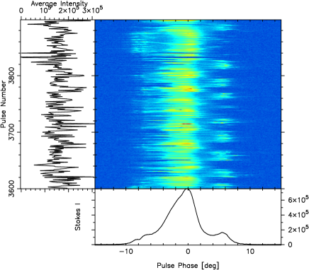
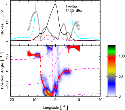
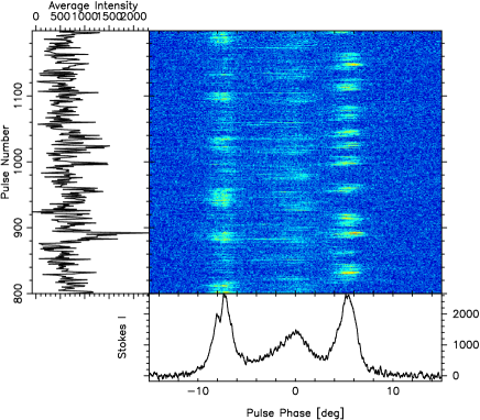
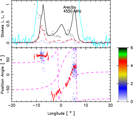
Figure 1: PSR B1946+35 pulse sequences (left hand displays) and average polarization characteristics (right hand displays) at 1.6 (LSP3) and 4.6 GHz (CPS1), respectively. The latter’s upper panels give the total intensity (Stokes $I$; solid curve), the total linear ($L$ [=$\sqrt{Q^{2}+U^{2}}$]; dashed red), the circular polarization (Stokes $V$; dotted blue), the fractional linear polarization ($L/I$; gray points) and a zoomed total intensity (10$\times I$; cyan curve). The PPA [=${1\over 2}\tan^{-1}(U/Q)$] densities (lower panels) within each 1$\degr$x1$\degr$-sample cell, corresponding to samples larger than 2 $\sigma$ in $L$, are plotted according to the color bars at the lower right, and have been derotated to infinite frequency. The average PPA traverses (red) are overplotted, and the RVM fit is plotted twice for the two polarization modes (magenta dashed) on each panel. The plot origins are taken at the fitted PPA inflection point.

Table 1: Details of the B1946+35 pulse sequences observed with the Arecibo telescope. The first four columns give the observing frequency, MJD and the Arecibo Project-ID, the raw time resolution, and the bandwidth. The fifth column gives the pulse-sequence range over which overlapping FFTs (of length OFFT in column 8) have been performed. The outside half-power pulse width measured for the full pulse sequence and the beam radius $\rho$ are given in columns 6 and 7. The fluctuation-frequency values $f_{3}^{offt}$ and $Q$ factor obtained for the corresponding range of pulses are given in columns 9 and 10.

Band	MJD/AO ProjID	Tres	BW	Range	Width	$\rho$	OFFT	$f_{3}^{offt}$	$Q=\frac{f_{3}^{offt}}{\Delta f}$
(GHz)		($\mu$s)	MHz	(pulses)	(∘)	(∘)		(c$P^{-1}$)
1.4	52837/P1734	1024	400	1–1366	15.6$\pm$0.1	4.6$\pm$0.1	256	0.0202$\pm$0.015	0.83
	(LPS1)			512–1262			256	0.0194$\pm$0.002	3.40
1.4	55632/P2532	512	400	1–1031	15.4$\pm$0.1	4.6$\pm$0.1	256	0.0238$\pm$0.002	1.45
	(LPS2)			512–1024			256	0.0239$\pm$0.002	2.93
1.4	57638/P3031	120	400	1–6678	15.5$\pm$0.1	4.6$\pm$0.1	256	0.0208$\pm$0.014	0.60
	(LPS3)			1250–1761			256	0.0193$\pm$0.003	3.21
				2500–3011			256	0.0235$\pm$0.003	3.85
				3550–4062			256	0.0312$\pm$0.002	6.11
				5100–5612			256	0.0314$\pm$0.002	6.63
4.6	57284/P2995	51	1187	1–1237	15.1$\pm$0.1	4.5$\pm$0.1	256	0.0104$\pm$0.029	0.34
	(CPS1)			520–776			256	0.0184$\pm$0.002	2.04

Note: Basic parameters for PSR B1946+35 are : dispersion measure DM = 129.07 ${\rm pc\,cm^{-3}}$, rotation measure RM=116 ${\rm rad\,m^{-2}}$,
period $P$ = 0.717 s, and period derivative $\dot{P}=7.061\times 10^{-15}$${\rm s\,s^{-1}}$.

The fluctuation spectra of the core features in S_t pulsars, on the other hand, show very different pulse-sequence modulation properties. ET III had established that the fluctuation spectra of most core-single pulsars were largely featureless. More recent analyses with more sensitive observations and analysis techniques largely reiterate this conclusion, though there is some evidence that in a few cases S_t pulsars exhibit diffuse fluctuation features (e.g., B0136+57, B0823+26, B1642–03 or B2255+58; see WES06, WES07; Basu et al. (2016)) with no discernible longitude motion, consistent with phase-stationary amplitude modulation. The conal components of pulsars with cores sometimes have sharper and steadier fluctuations with well defined $f_{3}$; however the modulation tends to be stationary in phase across the conal components. Importantly, pulsars with S_t profiles represent a younger population with slowdown rates $\dot{E}\raisebox{-1.29167pt}{\mbox{$\stackrel{{\scriptstyle>}}{{{}_{\sim}}}\,$}}10^{32}$ ${\rm ergs\,s^{-1}}$.

Here, we report an unusual type of pulse-sequence (hereafter PS) modulation in pulsar B1946+35. The pulsar is moderately bright and core-dominated when observed at L-band (1.4 GHz) but develops conal outriders at higher frequencies (e.g. Lyne & Manchester, 1988). PSR B1946+35 has been classified as having an S_t profile in ET IV and VI. Interestingly, single pulse fluctuation spectra studies at P-band (327 MHz) and L-band by WES06 and WES07 indicate strong modulation features across its pulse profiles. Furthermore, the studies also find very different $P_{3}$ values of 55$\pm$9$P$ (or $f_{3}\sim 0.018$ cycles $P^{-1}$ (hereafter c$P^{-1}$) where $P$ is the pulsar period) and 33$\pm$2 $P$(or $f_{3}\sim 0.030$ c$P^{-1}$) at P-band and L-band respectively, which the authors suggest may be due to the relatively short lengths of the observations that were perhaps insufficient to accurately estimate the average $P_{3}$ value.

In this paper, we use both archival and recent Arecibo observations to carry out a detailed study of this pulsar on a single pulse polarimetric basis. As we will illustrate, the pulsar’s fluctuation spectra suggest a highly periodic coupled modulation of both the core and conal emission, which is unusual for an S_t pulsar. We conclude that the pulsar’s modulation cannot be understood as subpulse drift within the usual rotating carousel subbeam model of RS75. How we reach this conclusion is the argument of this paper. In §2 we discuss the observations. §3 assembles the evidence pertaining to B1946+35’s profile classification and reviews the logic of our understanding it to be a core-single S_t pulsar. §4 discusses the fluctuation spectra and compares the results with known subpulse drift phenomena, and §5 gives the conclusion of this work.

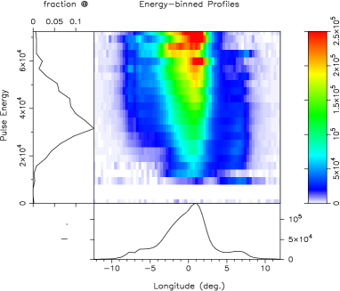
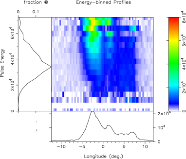
Figure 2: Intensity-fractionated displays for the LSP3 observation in Fig. 1 upper right: total power $I$ (left) and total linear $L$ (right). Note the pronounced shift to earlier longitudes of the higher intensity emission. This intensity-dependent aberration/retardation is responsible for the strange non-RVM “hook” in the PPA distribution between about –7 and –1° longitude. The effect is seen in $L$ as well as prominently in $I$ and is responsible for the unresolved double shape of the core component.

2 Arecibo Observations

The single pulse polarized pulse sequences for PSR B1946+35 were obtained with the 305-m Arecibo radio telescope in Puerto Rico together with its Gregorian reflector system and both the L-band-wide and C-band antenna-receiver systems. The observations were part of larger proposals which aimed to study the emission mechanism using single-pulse polarization observations of a large number of pulsars across multiple frequencies. The MJD and the Arecibo project ID for the observations used here are given in Table 1. The L-band pulse sequence observed on 17 July 2003/MJD 52837 (hereafter referred to as LPS1) was obtained using four WAPP (Wideband Arecibo Pulsar Processor) spectrometers, and the 12 March 2011/MJD 55632 and 7 September 2016/MJD 57638 (hereafter LPS2 and LPS3) observations used four Mock spectrometers with nominal 100- and 86-MHz bandwidths, respectively. The C-band pulse sequence (hereafter referred as CPS1) was observed on 19 September 2015/MJD 57284 using the seven Mock spectrometers with adjacent 170-MHz bands each. For each observation the raw Stokes parameters obtained for each band were corrected for dispersion and interstellar Faraday rotation. At L-band the three lower bands were found relatively free from interference and were thus added together to give an effective roughly 300-MHz bandwidth, whereas at C-band 3 bands were omitted owing to interference, giving an effective usable bandwidth of $\sim$ 600 MHz. Other relevant observing parameters are given in Table 1. Fig. 1 shows the single pulse sequence and polarization for the LPS3 and CPS1 observations. The L-band pulse sequence clearly shows periodic modulation for the central core and trailing conal component, while the modulation in the leading conal component is most clearly seen in the C-band observation.

3 Classification and Quantitative Geometry

Pulsar B1946+35 was classified as having a core-single (S_t) profile in ET VI, and its emission geometry was there modeled according to the RVM and core/double-cone models. Here, we review in detail the basis of this classification using all the available lines of evidence.

3.1 Profile and Spectral Evolution

Pulsar B1946+35 has a dispersion measure $DM$ of 129.07 ${\rm pc\,cm^{-3}}$, and its profile shows substantial scattering at meter wavelengths. Hence, only observations at higher frequencies are useful for studying the intrinsic emission properties of this pulsar. The spectral evolution of the average total power profile of PSR B1946+35 was published by Lyne & Manchester (1988) for 0.6, 1.6 and 2.6 GHz, and a 4.8-GHz profile appears in von Hoensbroech & Xilouris (1997). Our observations at L-band and C-band (see Fig. 1) have a significantly higher signal-to-noise ratio and are consistent with the earlier results. The primary characteristic of core-single (S_t) profile evolution is clearly seen in these observations. The pulsar’s profile has but a single bright component at 0.6 GHz; however, with increasing frequency two roughly symmetrical conal outriding components become ever more prominent until they are dominant at 4.8 GHz. Using our own 1.4-GHz observations, we estimate the half-power width of the central core component to be about $W_{c}$ = 5.0°$\pm$0.05°. The Gould & Lyne (1998) profiles provide a width measurement at 0.92 GHz of 5.4°$\pm$0.1°, and interpolating between 0.92 and 1.4 GHz, we obtain a 1-GHz core-component width of 5.2°$\pm$0.1°. Thus the geometrical interpretation of relating the core width to the polar cap size gives $\alpha\sim$32°. This is consistent with the $\alpha$ value estimated in papers ET IV and VI for this pulsar using core-width measurements from Rankin et al. (1989).

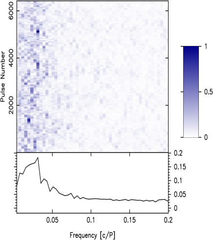
Figure 3: Display showing the time variations of the LRFS within the LPS3 pulse sequence. The top panel is a colour-coded representation with the longitude-averaged LRFS along the x-axis and increasing starting point along the y-axis. In order to closely show the observed spectral variations, the fluctuation scale is plotted only up to 0.2 c$P^{-1}$ (rather than the usual 0.5 c$P^{-1}$). The bottom panel shows the aggregate LRFSs along the y-axis (see §4 for details)

3.2 Polarimetry

The PPA histograms seen in the right-hand displays of Fig. 1 for the 1.4-GHz LPS3 and 4.6-GHz CPS1 observations appear at a first glance to be quite complex and inscrutable in RVM terms. They are complicated by orthogonal and non-orthogonal PPA modal jumps and swings. However for the LPS3 data, if the region between –7 and –1° longitude is ignored, a reasonable RVM traverse can be obtained that includes an orthogonal jump at +6° longitude. Mindful of the large correlation in fitting for $\alpha$ and $\beta$, we fitted instead for the steepest gradient point slope $R_{\rm pa}$ [$=\sin\alpha/\sin\beta$], obtaining a PPA rate of 16$\pm$3°/° and a PPA at the inflection point $PA_{0}$ of –66°$\pm$5°, both of which have well determined errors. The longitude origin of the lower plot in Fig. 2 corresponds to this inflection point and is also consistent with the point where the circular polarization changes sign. Using the $\alpha$ value of $\sim$32° from the core-width measurement together with the above $R_{\rm pa}$ value, we computed $\beta$ as 1.9°$\pm$0.3°. For the CPS1 observation in Fig. 1 the single pulses are weaker; however the PPA histogram is well sampled around –10° to –8° and 4° to 7° longitude showing that the values lie in approximately the same locations as in the LPS3 profile. Since the PPAs in these displays are derotated and thus reflect absolute orientations on the sky, the measurements indicate that the PPAs are frequency independent. The RVM measured for the upper LPS3 1.4-GHz observation, which is then imposed on the lower CPS1 4.6-GHz profile, then seems to be in good agreement with its average PPA traverse.

The steep PPA swing between –7 and –1° longitude is a curious feature that initially perplexed us. However, on closer inspection we noticed that the core feature is comprised of two blended, roughly Gaussian-like structures which together result in the asymmetric component. Analysis using intensity fractionation then revealed the intensity-dependent aberration/retardation that is responsible for the PPA “hook” as seen in Fig.  2. Similar PPA anomalies have now been identified and studied in the leading regions of bright core components of pulsars PSR B0329+54, B1237+25 and B1933+16 (Mitra et al., 2007; Smith et al., 2013; Mitra et al., 2016). There is some indication that the swing is produced by unequal mixing of orthogonal polarization-mode power occurring within that longitude range, however we were not able to make this case definitively for PSR B1946+35.

We now turn to an analysis of the pulsar’s basic emission geometry. Using the above $\alpha$ and $\beta$ values together with the measured widths at the outer half-power points of the conal component pair, we can compute the conal beam radius $\rho$. Following the spherical trigonometry methods of paper ET VI (eq. 4), this results in a value of approximately 4.6° around 1 GHz (the measured width and $\rho$ for all the observations are given in Table 1). This in turn is compatible with an inner cone geometry for a pulsar having a rotation period of 0.717 s (See also e.g. Gil et al., 1984). Note in addition that $\rho$ is practically constant between L-band and C-band, which is also an identifying inner cone property (ET VI & VII).

Thus, in summary, we have reestablished that pulsar B1946+35’s profile dimensions and polarization are consistent with a core-single (S_t) classification wherein the outriding conal components correspond to an inner cone geometry and the central component is well identified as a core emission feature. Assuming the outer half-power points to lie along last open field lines, one can define a parameter $s$ as the locus of the dipolar field line compared to polar fluxtube boundary such that $s=1$ corresponds to the edge of the open field region and $s=0$ is the beam center. Using the fact that the annular width of the cone is about 20% of the beam radius, the range of field lines over which the inner cone is illuminated in the beam is from $s\sim 1$ to $0.8$. Correspondingly the core emission illuminates field lines inwards of $s\sim 0.45$. This in turn ensures that the observer’s sightline through the beams is such that the core emission is relatively unaffected by any overlapping conal emission power.

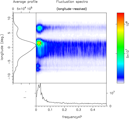
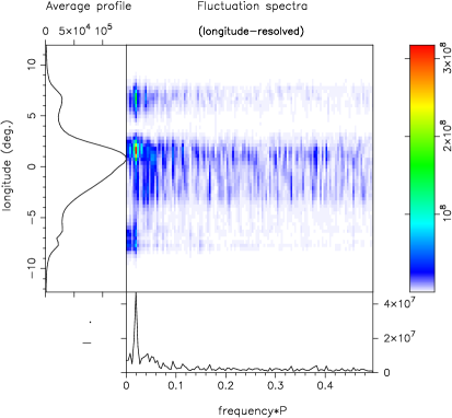
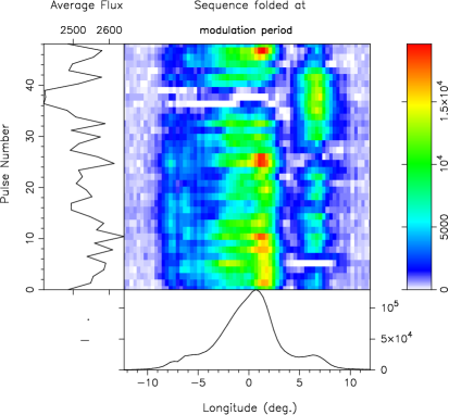
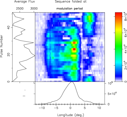
Figure 4: Total intensity, longitude-resolved fluctuation spectra using overlapping FFT lengths of 256 points (upper displays), modulation-phase plots (middle displays), and profiles folded at the modulation period (bottom) are given for the whole LPS3 observation (left) and for the 1250–1761 pulse interval (right). In the upper displays the main-panel fluctuation intensity is colour-coded according to the scale at the right, the average profile is given on the left and the aggregate intensity in the lower panel. The central displays show the average profiles, the fraction of modulated power (dashed curve) and the phase function (lower panels). Displays at the bottom show the character of profile changes over the modulation cycle (main panel, colour-code per the scale at the right); the total power fluctuation is shown at the left and the constant “base” profile at the bottom (see §4 for details).

4 Fluctuation Spectral Analysis

A clear suggestion of periodic fluctuations in PSR B1946+35 can be seen in the single pulse sequences of Fig. 1 both at L-band and C-band. This was also implicit in the fluctuation spectra analyses of WES06 and WES07. Such behavior is unusual for a core-single pulsar. In order to investigate the character of these fluctuations in more detail we proceeded to compute longitude-resolved fluctuation spectra (hereafter LRFS) for this pulsar in a number of different ways. WES06 and WES07 found two different $f_{3}$ values using short intervals of P- and L-band observations. We wondered if this difference could result from a time-varying fluctuation property of the pulsar, and this prompted us to first look for temporal variations in the long LPS3 sequence using techniques similar to those described by Basu et al. (2016). In this method LRFSs of 256 pulses were computed as a function of time after shifting the starting pulse successively by ten periods. For every time realization, the LRFSs were averaged across pulse longitude such that a single fluctuation spectrum was obtained, and finally after shifting each by ten periods these LRFSs were represented on a two dimensional map. This map was normalized to unity and is shown as a colour-coded distribution in the top panel of Fig. 3, where the ordinate corresponds to the starting pulse for computing LRFSs and the abscissa to the LRFSs frequency in c$P^{-1}$. The display in the bottom plot of Fig. 3 shows the average LRFS after collapsing all the LRFSs along the vertical axis.

Remarkably, an interesting pattern was observed in the temporal variations of the LRFS, where for about thousand pulses the LRFS shows a broad low frequency “red” power excess, but it then suddenly exhibits a very different behavior for a few hundred pulses characterized by a highly periodic modulation. We looked for this effect in the shorter LPS1, LPS2 and CPS1 observations, and found intervals having similar broad low frequency excesses and also sections with highly periodic modulations. To further quantify this effect we resorted to analyzing sections of the observations by performing overlapping 256-point FFTs (see Deshpande & Rankin 2001 for the method). We found that the LRFS for each entire pulse sequence revealed the broad low frequency excess, and we extracted a characteristic fluctuation frequency by fitting the parametric Bézier curve to the average LRFS and locating the peak frequency of this fitted curve which we will refer to as $f_{3}^{offt}$.

For highly modulated periodic intervals of the pulse sequences we fitted a cubic spline to the sharp spectral feature to find the corresponding peak $f_{3}^{offt}$ values. The sharpness of the spectral feature was estimated by computing a “quality factor” $Q=f_{3}^{offt}/\Delta f$, where $\Delta f$ corresponds to the half-power width of the feature. The range of pulses over which the FFTs were computed, the number of points for the overlapping FFTs, values of $f_{3}^{offt}$ in c$P^{-1}$, and Q factors for all the sequences are quoted in Table 1. The errors in $f_{3}^{offt}$ were estimated using eq.(4) of Basu et al. (2016). Note that these highly modulated features appear at three distinct frequencies, although they are not harmonically related to each other.

The LRFS analysis described above reveals $f_{3}^{offt}$ values in sections of the observations which are similar to the two different values found by WES06 and WES07 at two different observing frequencies. For example two pulse ranges from the LPS3 observation, one in the interval 3550–4062 had $f_{3}^{offt}$=0.0312$\pm$0.003 c$P^{-1}$, which is comparable to the L-Band WES06 value of 0.031 (their $P_{3}$=$33\pm 2$$P$), while another interval 1250–1761 had $f_{3}^{offt}$=0.0193$\pm$0.003 c$P^{-1}$, which is similar to the WES07 P-band value of 0.018 (their $P_{3}$=$55\pm 9$$P$). Thus we conclude that the variation in the modulation frequency reported earlier is not frequency dependent, but rather occurs at different times when the pulsar is observed at any frequency.

The intervals of periodic modulation in the observations are seen not only in the two conal components, but also in regions on both sides of the core component. In Fig. 4 we show the results of detailed LRFS analyses of the full LPS3 pulse sequence (left column) and the pulse range 1250–1761 (right column). The top panels show the LRFS, the middle displays plot the amplitude and phase of the spectral feature across the longitude range of the pulse profile, and the bottom panels show the pulse sequence folded at the $f_{3}^{offt}$ frequency as given in Table 1. Notice that in the LRFS for the entire pulse sequence the average spectral feature (lower panel) is broad and diffuse in nature, but is clearly seen to fluctuate in both the core and conal profile regions. However, within the specific interval where the pulse sequence displays periodic modulation, the narrow spectral feature $f_{3}^{offt}$ is clearly seen across the profile.

The peak signal-to-noise ratio (S/N) of the feature is about 100 (the noise being calculated in higher frequency regions between 0.3 to 0.35 c$P^{-1}$ where the spectum is featureless and dominated by white noise), and the power up to the half-power point is confined to a single FFT frequency component giving a factor $Q=f_{3}^{offt}/\Delta f\sim 3.2$ (see Table 1). The middle displays show the average amplitude and phase of the spectral feature across the longitude range of the pulse profile. The amplitude under the leading component shows the least fluctuating power, whereas the trailing part of the core component is more strongly modulated than the leading part and is similar in magnitude to that of the trailing component. The modulation phase is remarkably constant across each component implying that the fluctuations correspond to pure amplitude modulation. The leading conal component and the core region are modulated very closely in phase, whereas the trailing component is modulated almost precisely in counter phase. These various aspects of the periodic modulation can also be seen in the bottom displays of Fig. 4, where the pulse sequence has been folded at the $f_{3}^{offt}$ frequency. Here we see that for a 24-25$P$ half-portion of the modulation cycle, the pulsar’s leading conal and core components are active, and then for the remaining half of the cycle, these weaken and the bright trailing conal component appears and stays active. The corresponding harmonic-resolved fluctuation spectrum (HRFS, see Deshpande & Rankin 2001; Basu et al. 2016) which lies in 0–1 c$P^{-1}$ range provides an alternative way of determining the phase behaviour of the fluctuating feature. The feature in the HRFS (not shown) lies symmetrically about the center point 0.5 c$P^{-1}$ which indicates that the responses represent largely amplitude modulation as expected.

5 Comparison with Other Pulsar Modulation Phenomena

Over time scales of few thousand pulses radio pulsars are well known to exhibit three major types of pulse-sequence effects: subpulse drifting, pulse nulling, and mode-changing (e.g., see ET III). Amongst these, high Q periodic modulation is primarily seen in the subpulse-drifting phenomenon. The periodicities found are typically longer than the pulsar rotation period $P$ and can be as long as a few tens of seconds. The fluctuation-spectral analyses described above for B1946+35 suggest periodic modulation of about 35 s, and we now contrast its properties with the subpulse-drift phenomenon.

High Q drift features are seen primarily in conal single S_d pulsars, where the fluctuation is associated with distinct phase modulation across the pulse profile. In some situations high Q periodic stationary or amplitude modulation is observed in conal component pairs [e.g., PSR B1857–26 (Mitra & Rankin, 2008); B1237+25 (Smith et al., 2013) and B2045–16 (Basu et al., 2016)] which correspond to conal double profiles with central sightline traverses. In all these cases however, the central core emission never seems to show any high Q periodic modulation. This geometrical property of the drifting-subpulse phenomenon has given rise to the carousel model, wherein the drifts of the conal emission are understood as due to a persistent system of localized beamlets which rotate on a roughly circular path around the dipolar magnetic axis. The core emission is associated with a beam which is anchored near the dipole axis and hence is phase stationary. We have questioned whether the regular modulation in B1946+35 might be due to some kind of carousel-beam system, and such a mechanism for the conal fluctuations cannot be entirely ruled out. However, the joint modulation of B1946+35’s well identified core emission together with that of the cones is unusual and paradoxical here. If we insist that the observed modulation results from moving beamlets that cross our sightline, then both the conal and core beamlets should be moving perpendicular to the sightline circle—and thus in contradiction with the carousel model.

The physical motivation for the carousel model was outlined by RS75, where they suggested that an inner vacuum gap (IVG) exists near the pulsar polar cap which discharges as a set of the localized sparks. Through a complex process of electron-positron pair creation, a spark-generated relativistic plasma flow is established which gives rise to the radio emission at altitudes of a few hundred kilometers above the neutron star surface. Hence each spark is associated with a plasma column and appears as a beamlet in the emission region. Due to E$\times$B drift in the IVG, the sparks experience a slow (magnetic azimuthal) drift which lags the pulsar corotation. As a result the radio emitting beamlets also lag the corotation, and this gives rise to the subpulse drifting phenomenon. In an LRFS analysis, the modulation frequency $f_{3}^{offt}$ can be interpreted in terms of the spark repetition time $P_{3}$. RS75 explored this problem for an antipulsar where the rotation and magnetic axes are aligned and hence the beamlet motion is both around the rotation and magnetic axes—and this is the genesis of the carousel model. Application of this model to actual pulsars—where their rotation and magnetic axes are necessarily non-aligned—is far from trivial. While there has been observational support for the carousel model wherein the sparks rotate around the magnetic axis, Basu et al. (2016) have recently pointed out that the model is inconsistent physically with the fundamental circumstance that sparks must lag behind a pulsar’s corotation.

The lack of any significant periodic modulation in pulsar core emission has been the most stringent observational constrain on the carousel model, since the core has been interpreted as a stationary (non-drifting) beam located along the dipolar magnetic axis. However, the modulation we observe in the core of B1946+35 breaks that constraint. One key question then naturally arises: can some refinement of the RS75 spark-drifting model explain the host of drifting phenomena observed, including both the phase and amplitude modulation of periodic fluctuations. Recently, in an effort to resolve this problem, Basu et al. (2016) and Szary (2013) suggested that if the magnetic field in the IVG is highly non-dipolar, then the motion of sparks lagging the corotation in the IVG can produce both phase- and amplitude-stationary modulation in the dipolar radio-emission region. However, it is too early to conclude whether this idea can explain the broad range of observed subpulse-drift properties.

There is also another aspect of drifting that needs attention while interpreting the PSR B1946+35 modulation. Recently Basu et al. (2016) carefully applied the RS75 conception that sparks lag behind pulsar corotation, and they found that pulsars with phase- and amplitude-modulated drifting could be seen as two separate populations in $\dot{E}$ space: One group of pulsars with with both phase and amplitude drift modulation are seen to lie below $\dot{E}\sim$ 2$\times$10³² ${\rm ergs\,s^{-1}}$, and the drift periodicity $P_{3}$ was found to be anti-correlated with $\dot{E}$ roughly as $P_{3}\sim$ ($\dot{E}/2$$\times$10${}^{32})^{-0.6}P$; whereas the other group for which $\dot{E}>$ 2$\times$10³² ${\rm ergs\,s^{-1}}$ all showed only amplitude modulation with a median value of $P_{3}\sim$ 30$\pm$15 $P$. Basu et al. (2016) interpreted this fascinating result using a partially screened vacuum gap or PSG model (Gil et al., 2003)—which is the modified RS75 model wherein the IVG is partially screened due to presence of ions that are extracted from the neutron-star surface. They demonstrated that under the PSG model, the $P_{3}$ vs. $\dot{E}$ anticorrelation can be explained as an increase in the spark drift speed with increasing $\dot{E}$ of the pulsar. This also means that above a certain $\dot{E}$, when $P_{3}$ becomes less than the $P$, subpulse-drift motion is aliased and cannot any longer be observed. This then raises the question as to what is the physical origin of the phase-stationary amplitude modulation seen in the group two pulsars. PSR B1946+35 has an $\dot{E}\sim$ 7.6$\times$10³² ${\rm ergs\,s^{-1}}$, and lies in group two. Its phase-stationary periodic modulation could then be an entirely new phenomenon.

Similarly, the phenomenon known as “mode changing”—wherein a pulsar’s average profile assumes several different discrete forms and the individual pulse properties so change to produce them—is well documented in a variety of different pulsars. In several of the early exemplars of mode-changing (e.g., B0329+54 and B1237+25) the effect took the form of a change in the symmetry of the conal component emission about the central core component, and this description surely could be taken to apply to B1946+35 as well, although in this case the changes occur on a significantly shorter time scale of about 18 s. The other problem is that mode-changing is not known to be periodic, and surely not periodic with a reasonably high $Q$ as we see in this pulsar.

The high Q drift feature in pulsars is known to show gradual changes across a particular mode (e.g. B0943+10, see Rankin & Suleymanova, 2006) or when the pulsar recovers from its nulling phase (e.g. B0809+74 van Leeuwen et al. 2002). In certain drifters like B0031–07 (Vivekanand & Joshi, 1997; Smits et al., 2005; McSweeney et al., 2017), B1944+17 (Kloumann & Rankin, 2010), B1918+19 (Rankin et al., 2013) and B2319+60 (Wright & Fowler, 1981) the high Q modulation feature is seen to have multiple (often three) distinct high Q modulation frequencies often interspersed with long duration nulling episodes. In this context it is interesting to note that PSR B1946+35 switches into a high Q mode after spending long intervals in a mode marked by low frequency excess. For the long L-band observation, we found that the pulsar can settle into three distinct high Q periodicities as seen in Fig. 3 and Table 1.

Indeed, overall it is conal emission that exhibits well established periodicities, not cores. Core radiation more typically presents as “white” noise in flat or featureless fluctuation spectra. A few examples of long broad periodicities in core components are known (e.g., Rankin 1986,WES06, WES07), though very few have been studied in detail and documented. In pulsar B1237+25, the core-associated periodicity seems to be associated with its three modes (Srostlik & Rankin, 2005), where in the “quiet normal” mode core “flares” are observed at rough intervals of some 60 periods. Core eruptions also seem responsible for the “red noise” (noted in the first paper above) in the central regions of several classical conal double pulses, though no clear periodicities have so far been established (Young & Rankin, 2012). It begins to seem that core fluctuations might be a more widespread phenomenon and needs further investigation.

Recently, several new quasiperiodic bursting phenomena, akin to mode changes, have been identified in radio pulsar emission—e.g., PSR J1752+2359 (Lewandowski et al., 2004); J1938+2213 (Lorimer et al., 2013); B0611+22 (Seymour et al., 2014). For PSR B0611+22 Rajwade et al. (2016) explored whether there might be simultaneous X-ray emission changes during its radio mode changes. However, they did not detect X-ray emission from this pulsar, and hence the mode changes could not be associated with magnetospheric “states” as have been observed for the radio and X-ray mode changing pulsar B0943+10 (Hermsen et al., 2013; Mereghetti et al., 2016). Another quasiperiodic phenomenon has been studied in pulsars B0919+06 and B1859+07 with bistable behaviour (Rankin et al., 2006; Han et al., 2016; Wahl et al., 2016), wherein occasionally the bright emission window shifts earlier for a few or several score periods and then returns to its usual phase. This resembles in several ways the emission pattern seen in PSR B1946+35, where for about 25 $P$ the pulsar’s emission window corresponding to the leading conal and core component appears shifted, followed by an active phase of similar duration for the trailing conal component. However, the timescales of these bursting or bistable phenomena (see also Lyne et al., 2010) are larger or much larger than the B1946+35 modulation period. Interestingly, Wahl et al. (2016) explore whether the bistable quasi-periodicity could arise due to the emission being affected in a periodic manner by a ‘satellite’ object rotating in a binary system. Given the observed modulation periodicities of about 300 s and 100 s in B0919+06 and B1859+07, they found that the semi-major axis of the companion should be at a distance comparable to the light cylinder and have densities larger than $10^{5}$ ${\rm gm\,cm^{-3}}$ to avoid tidal disruptions. We however do not advocate such a mechanism for PSR B1946+35, with a modulation period of only some 36 s, thus making the orbit fall well within the light cylinder.

6 Conclusion

As argued above the highly periodic phase-stationary fluctuations in intervals of pulsar B1946+35’s modulation cannot be reconciled with the drifting-subpulse phenomenon in any conceivable geometrical context. The periodic fluctuations in this pulsar appear to require some sort of emission-pattern changing on timescales of about 18 s. How this new effect may or may not be related to the well known mode-changing phenomenon remains unclear. Mode changes have generally been documented through use of modal profiles computed over much longer time intervals, and periodicities have not heretofore been documented as an aspect of this phenomenon. Longer duration observations at multiple frequency bands will throw more light on the nature of this new phenomenon.

References

- Backer (1970) Backer D. C., 1970, Nature, 227, 692
- Basu et al. (2016) Basu R., Mitra D., Melikidze G. I., Maciesiak K., Skrzypczak A., Szary A., 2016, Ap.J., 833, 29
- Blaskiewicz et al. (1991) Blaskiewicz M., Cordes J. M., Wasserman I., 1991, Ap.J., 370, 643
- Cordes (1979) Cordes J. M., 1979, Australian Journal of Physics, 32, 9
- Deshpande & Rankin (2001) Deshpande A. A., Rankin J. M., 2001, MNRAS, 322, 438
- Gil & Sendyk (2000) Gil J. A., Sendyk M., 2000, Ap.J., 541, 351
- Gil et al. (1984) Gil J., Gronkowski P., Rudnicki W., 1984, A&A, 132, 312
- Gil et al. (2003) Gil J., Melikidze G. I., Geppert U., 2003, A&A, 407, 315
- Gil et al. (2004) Gil J., Lyubarsky Y., Melikidze G. I., 2004, Ap.J., 600, 872
- Gould & Lyne (1998) Gould D. M., Lyne A. G., 1998, MNRAS, 301, 235
- Han et al. (2016) Han J., et al., 2016, MNRAS, 456, 3413
- Hankins et al. (2003) Hankins T. H., Kern J. S., Weatherall J. C., Eilek J. A., 2003, Nature, 422, 141
- Hermsen et al. (2013) Hermsen W., et al., 2013, Science, 339, 436
- Kloumann & Rankin (2010) Kloumann I. M., Rankin J. M., 2010, MNRAS, 408, 40
- Komesaroff (1970) Komesaroff M. M., 1970, Nature, 225, 612
- Kramer et al. (2006) Kramer M., Lyne A. G., O’Brien J. T., Jordan C. A., Lorimer D. R., 2006, Science, 312, 549
- Lewandowski et al. (2004) Lewandowski W., Wolszczan A., Feiler G., Konacki M., Sołtysiński T., 2004, Ap.J., 600, 905
- Lorimer et al. (2013) Lorimer D. R., Camilo F., McLaughlin M. A., 2013, MNRAS, 434, 347
- Lyne & Manchester (1988) Lyne A. G., Manchester R. N., 1988, MNRAS, 234, 477
- Lyne et al. (2010) Lyne A., Hobbs G., Kramer M., Stairs I., Stappers B., 2010, Science, 329, 408
- McLaughlin et al. (2006) McLaughlin M. A., et al., 2006, Nature, 439, 817
- McSweeney et al. (2017) McSweeney S. J., Bhat N. D. R., Tremblay S. E., Deshpande A. A., Ord S. M., 2017, preprint, (arXiv:1701.06755)
- Melrose (1995) Melrose D. B., 1995, Journal of Astrophysics and Astronomy, 16, 137
- Mereghetti et al. (2016) Mereghetti S., et al., 2016, Ap.J., 831, 21
- Mitra & Deshpande (1999) Mitra D., Deshpande A. A., 1999, A&A, 346, 906
- Mitra & Li (2004) Mitra D., Li X. H., 2004, A&A, 421, 215
- Mitra & Rankin (2008) Mitra D., Rankin J. M., 2008, MNRAS, 385, 606
- Mitra et al. (2007) Mitra D., Rankin J. M., Gupta Y., 2007, MNRAS, 379, 932
- Mitra et al. (2015) Mitra D., Arjunwadkar M., Rankin J. M., 2015, Ap.J., 806, 236
- Mitra et al. (2016) Mitra D., Rankin J., Arjunwadkar M., 2016, MNRAS, 460, 3063
- Radhakrishnan & Cooke (1969) Radhakrishnan V., Cooke D. J., 1969, Astrophys. Lett., 3, 225
- Rajwade et al. (2016) Rajwade K., Seymour A., Lorimer D. R., Karastergiou A., Serylak M., McLaughlin M. A., Griessmeier J.-M., 2016, MNRAS, 462, 2518
- Rankin (1983) Rankin J. M., 1983, Ap.J., 274, 333
- Rankin (1986) Rankin J. M., 1986, Ap.J., 301, 901
- Rankin (1993a) Rankin J. M., 1993a, Ap.J. Suppl., 85, 145
- Rankin (1993b) Rankin J. M., 1993b, Ap.J., 405, 285
- Rankin & Suleymanova (2006) Rankin J. M., Suleymanova S. A., 2006, A&A, 453, 679
- Rankin et al. (1989) Rankin J. M., Stinebring D. R., Weisberg J. M., 1989, Ap.J., 346, 869
- Rankin et al. (2006) Rankin J. M., Rodriguez C., Wright G. A. E., 2006, MNRAS, 370, 673
- Rankin et al. (2013) Rankin J. M., Wright G. A. E., Brown A. M., 2013, MNRAS, 433, 445
- Ruderman & Sutherland (1975) Ruderman M. A., Sutherland P. G., 1975, Ap.J., 196, 51
- Seymour et al. (2014) Seymour A. D., Lorimer D. R., Ridley J. P., 2014, MNRAS, 439, 3951
- Smith et al. (2013) Smith E., Rankin J., Mitra D., 2013, MNRAS, 435, 1984
- Smits et al. (2005) Smits J. M., Mitra D., Kuijpers J., 2005, A&A, 440, 683
- Srostlik & Rankin (2005) Srostlik Z., Rankin J. M., 2005, MNRAS, 362, 1121
- Szary (2013) Szary A., 2013, preprint, (arXiv:1304.4203)
- Vivekanand & Joshi (1997) Vivekanand M., Joshi B. C., 1997, Ap.J., 477, 431
- Wahl et al. (2016) Wahl H. M., Orfeo D. J., Rankin J. M., Weisberg J. M., 2016, MNRAS, 461, 3740
- Wang et al. (2007) Wang N., Manchester R. N., Johnston S., 2007, MNRAS, 377, 1383
- Weltevrede et al. (2006) Weltevrede P., Edwards R. T., Stappers B. W., 2006, A&A, 445, 243
- Weltevrede et al. (2007) Weltevrede P., Stappers B. W., Edwards R. T., 2007, A&A, 469, 607
- Wright & Fowler (1981) Wright G. A. E., Fowler L. A., 1981, A&A, 101, 356
- Young & Rankin (2012) Young S. A. E., Rankin J. M., 2012, MNRAS, 424, 2477
- van Leeuwen et al. (2002) van Leeuwen A. G. J., Kouwenhoven M. L. A., Ramachandran R., Rankin J. M., Stappers B. W., 2002, A&A, 387, 169
- von Hoensbroech & Xilouris (1997) von Hoensbroech A., Xilouris K. M., 1997, A&A Suppl., 126