Indirect searches of Galactic diffuse dark matter in INO-MagICAL detector

Abstract

The signatures for the existence of dark matter are revealed only through its gravitational interaction. Theoretical arguments support that the Weakly Interacting Massive Particle (WIMP) can be a class of dark matter and it can annihilate and/or decay to Standard Model particles, among which neutrino is a favorable candidate. We show that the proposed 50 kt Magnetized Iron CALorimeter (MagICAL) detector under the India-based Neutrino Observatory (INO) project can play an important role in the indirect searches of Galactic diffuse dark matter in the neutrino and antineutrino mode separately. We present the sensitivity of 500 kt$\cdot$yr MagICAL detector to set limits on the velocity-averaged self-annihilation cross-section ($\langle\sigma v\rangle$) and decay lifetime ($\tau$) of dark matter having mass in the range of 2 GeV $\leq m_{\chi}\leq$ 90 GeV and 4 GeV $\leq m_{\chi}\leq$ 180 GeV respectively, assuming no excess over the conventional atmospheric neutrino and antineutrino fluxes at the INO site. Our limits for low mass dark matter constrain the parameter space which has not been explored before. We show that MagICAL will be able to set competitive constraints, $\langle\sigma v\rangle\leq 1.87\,\times\,10^{-24}$ cm³ s^-1 for $\chi\chi\rightarrow\nu\bar{\nu}$ and $\tau\geq 4.8\,\times\,10^{24}$ s for $\chi\rightarrow\nu\bar{\nu}$ at 90$\%$ C.L. (1 d.o.f.) for $m_{\chi}$ = 10 GeV assuming the NFW as dark matter density profile.

1 Introduction and Motivation

Plethora of attempts are being made in the intensity, energy, and cosmic frontiers to build up knowledge about the Universe. Recent observations by Planck satellite Ade:2015xua confirm that the baryonic and unknown non-baryonic matter (dark matter) contribute $\sim$ 4.8$\%$ and $\sim$ 26$\%$ of the total energy density of the Universe respectively. The first indication for the existence of dark matter (DM) in the Universe was made by the Swiss astronomer Fritz Zwicky Zwicky:1933gu . This observation was put on a solid footing by Vera Rubin and her collaborators Rubin:1970zza . The astrophysical Strigari:2013iaa ; Clowe:2006eq and cosmological observations Komatsu:2014ioa ; Steigman:2012ve confirm the existence of dark matter from the length scales of a few kpc to a few Gpc.

All the astrophysical evidences of dark matter are through its gravitational interactions. The non-gravitational particle physics properties of DM particles are completely unknown. The relic abundance of cold dark matter (CDM) in the Universe is matched assuming a $\sim$100 GeV dark matter particle with electro-weak coupling strength. This class of particles is known as Weakly Interacting Massive Particle (WIMP) Jungman:1995df ; Bertone:2004pz ; Bergstrom:2000pn . Supersymmetry, one of the most favored beyond-the-Standard Model theory, also predicts more than one dark matter candidates including the WIMP Ellis:2010kf .

There are three types of detection methods for the search of DM: (i) Direct detection: DM particles are detected by observing recoiled nuclei from the scattering of DM particles in the laboratory. Experiments such as DAMA/LIBRA Bernabei:2010mq , LUX Akerib:2015rjg , CDMS Agnese:2015nto , XENON Aprile:2012nq , DarkSide Agnes:2015ftt , and PandaX Xiao:2015psa pursue this strategy. (ii) Indirect detection: It is possible that DM particles can decay and/or annihilate to any of the Standard Model (SM) particles like $\nu\bar{\nu}$, $t\bar{t}$, $b\bar{b}$ etc. An excess (over standard astrophysical backgrounds) of these SM particles can be searched for to understand dark matter. The unstable SM particles decay to produce neutrinos and photons which can be searched for indirect detection. The prospects of dark matter searches through neutrino portal has been studied in the literature Lindner:2010rr ; Agarwalla:2011yy ; Farzan:2011ck ; Mijakowski:2011zz ; Blennow:2013pya ; Gustafsson:2013gca ; Aisati:2015ova ; Anchordoqui:2015lqa ; Arina:2015zoa ; Macias:2015cna ; Gonzalez-Macias:2016vxy ; Zornoza:2016ggm ; Garcia-Cely:2017oco ; Beacom:2006tt ; Yuksel:2007ac . Fermi-LAT presents the analysis of its collected data of gamma rays having the energy in the range of 200 MeV to 500 GeV from Galactic halo in 5.8 years in Ref. Ackermann:2015lka . Multiwavelength searches for dark matter have complementary reach Laha:2012fg . Our focus in this work is indirect detection of dark matter via neutrinos and antineutrinos. (iii) Collider searches: The searches for supersymmetric DM candidates are carried out in LHC Khachatryan:2015bbl ; Chatrchyan:2012tea ; Aad:2012fw .

The 50 kt Magnetized Iron CALorimeter (MagICAL) detector is proposed to be built by the India-based Neutrino Observatory (INO) project to observe the atmospheric neutrino and antineutrino separately having energy in multi-GeV range and covering a wide ranges of path lengths (few km to few thousands of km) through the Earth matter. The primary mission of the MagICAL detector is to unravel the mass ordering (MO) of neutrino using the Earth matter effect Ghosh:2012px ; Devi:2014yaa ; Ahmed:2015jtv ; Mohan:2016gxm and to measure the neutrino mixing parameters precisely Thakore:2013xqa ; Kaur:2014rxa ; Devi:2014yaa . The MagICAL detector has also the potential to explore the physics beyond the Standard Model Dash:2014fba ; Chatterjee:2014oda ; Chatterjee:2014gxa ; Choubey:2015xha ; Behera:2016kwr . In our study, we show that the MagICAL detector can play a very important role in the indirect search of DM having mass in the multi-GeV range with the help of its excellent detection efficiency, energy, and angular resolutions. We explore the sensitivity of the MagICAL detector to detect the neutrino and antineutrino events coming from the diffuse dark matter annihilation/decay in the Milky Way galaxy. We present the constraint on the self-annihilation cross-section ($\langle\sigma v\rangle$) and the decay lifetime ($\tau$) of diffuse dark matter having mass in the range [2, 90] GeV and [4, 180] GeV respectively using 500 kt$\cdot$yr exposure of the MagICAL detector.

We describe the dark matter density profile and the calculation of annihilation and decay rate of dark matter in section 2. The key features of the MagICAL detector is presented in section 3. Section 4 deals with the expected event distribution of atmospheric and DM induced neutrinos in the MagICAL detector. We present the simulation method in section 5. The prospective limits on the self-annihilation cross-section and decay lifetime of dark matter are presented in section 6. We compare our results with the existing bounds from other experiments. We also study the flux upper limit due to dark matter induced neutrinos in the MagICAL detector. We conclude in section 7.

2 Discussions on dark matter

2.1 Dark matter density profile

The general parameterization of a spherically symmetric dark matter density profile is given by

$$\rho(r)=\frac{\rho_{0}}{\big{[}\delta\,+\,r/r_{s}\big{]}^{\gamma}\,.\,\big{[}1+(r/r_{s})^{\alpha}\big{]}^{(\beta-\gamma)/\alpha}}\,.$$ (1)

The density, $\rho(r)$, is expressed in GeV cm^-3 and $\it{r}$ is the distance from the center of the galaxy in kpc. The parameter, $r_{s}$, is the scale radius in kpc. The shape of the outer profile is controlled by $\alpha$ and $\beta$, whereas $\gamma$ parametrizes the slope of the inner profile. The dark matter density at the Solar radius (R_sc) is denoted by $\rho_{sc}$. We assume R_sc = 8.5 kpc 2016arXiv161002457D . The normalization constant, $\rho_{0}$, and all the results are calculated using the values of parameters as given in table 1.

Numerical simulations which involve only dark matter particles predict a cuspy profile Navarro:1995iw ; Diemand:2006ik ; Stadel:2008pn ; Navarro:2008kc . Although these simulations reproduce the large-scale structure of the Universe, yet this prescription has challenges at scales below the size of a typical galaxy. It has been proposed that the addition of baryons can solve all of these small scale issues, although the results vary Stinson:2012uh ; DiCintio:2013qxa ; Tollet:2015gqa ; Chan:2015tna ; Marinacci:2013mha ; Kim:2013jpa ; Schaye:2014tpa ; Schaller:2014uwa ; Sawala:2015cdf . Present observations are not yet precise enough to distinguish between a cored and a cuspy profile Cerdeno:2016znc .

To take this DM halo uncertainty into account, we generate all the results with two different DM profiles: Navarro Frenk White (NFW) profile  Navarro:1995iw , which represents cuspy halos, and the Burkert profile 1999dmap.conf..375B , which represents cored halos. The values of different parameters associated with these profiles are taken from Ref. Aartsen:2015xej . In Fig. 1(a), we plot the NFW and Burkert dark matter density profiles with distance $r$  from the center of the Milky Way galaxy by the black solid and green dashed lines respectively.

For conservativeness, we do not consider the effects of dark matter substructure. Depending on the value of the minimum halo mass and other astrophysical uncertainties, this can give a substantial contribution to the signal discussed here Ando:2005hr ; Ng:2013xha ; Campbell:2014bca ; Correa:2015dva ; Bartels:2015uba ; Moline:2016pbm .

	($\alpha,\beta,\gamma,\delta$ )	$\rho_{sc}$ [GeV cm-3]	$r_{s}$ [kpc]
NFW	(1, 3, 1, 0)	0.471	16.1
Burkert	(2, 3, 1, 1)	0.487	9.26

Table 1: The value of parameters associated with the NFW and Burkert profiles are listed here. They are same as in Ref. Aartsen:2015xej .

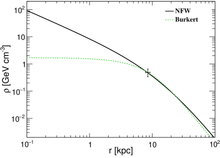
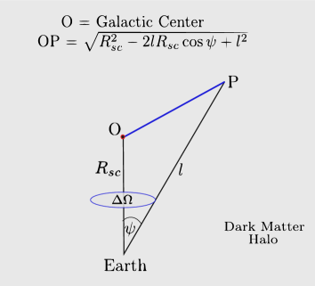
Figure 1: (a) Distribution of the dark matter density in the Milky Way galaxy for the NFW (black solid line) and Burkert profiles (green dashed line). The observational bounds on local dark matter density ($\rho_{sc}$) and the solar radius ($R_{sc}$) and their 2$\sigma$ uncertainties are indicated Strigari:2013iaa ; Aartsen:2015xej . (b) A schematic diagram of some part of the Milky Way dark matter halo. The Galactic center (GC) is denoted by O and $R_{sc}$ is the distance between the Earth and the GC. The parameter $l$ is the distance between point P and the Earth. The angle made at the Earth by points P and O and the corresponding solid angle are denoted by $\psi$ and $\Delta\Omega$ respectively.

In Fig. 1(b), a schematic diagram of a small portion of the Milky Way DM halo is shown with O as the Galactic center (GC). The dark matter density at point P with its distance $l$ from the Earth is a function of the length OP = $\sqrt{R_{sc}^{2}-2lR_{sc}\cos\psi+l^{2}}$. The angle made at the Earth by points P and O is $\psi$ and the corresponding solid angle is $\Delta\Omega$.

2.2 Annihilation of dark matter

We consider the annihilation between a dark matter particle ($\chi$) and its antiparticle ($\bar{\chi}$) to produce a neutrino and an antineutrino in the final state with 100$\%$ branching ratio:

$$\chi+\bar{\chi}\rightarrow\nu+\bar{\nu}\,.$$ (2)

The neutrinos and antineutrinos of $e$, $\mu$, and $\tau$ flavors are assumed to be produced in 1:1:1 ratio at source. This ratio remains same on arrival at the Earth surface due to loss of coherence while propagating through astrophysical distances (see appendix A).

The number of $\nu/\bar{\nu}$ from a direction $\psi$ due to the annihilation of dark matter particles is proportional to the line of sight integration of the square of dark matter density:

$$\mathcal{J}^{ann}(\psi)=\frac{1}{R_{sc}\rho^{2}_{sc}}\int_{0}^{l_{max}}dl\,\,\rho^{2}\left(\sqrt{R_{sc}^{2}-2lR_{sc}\cos\psi+l^{2}}\right)\,.$$ (3)

The factor $\frac{1}{R_{sc}\rho^{2}_{sc}}$ is included to make $\mathcal{J}^{ann}(\psi)$ dimensionless. The upper limit $l_{max}$ is the distance between the observer and the farthest point (denoted by P^′) in the Milky Way halo at the angle $\psi$. The radius of Milky Way galaxy is $R_{\rm MW}$ (= OP^′ = 100 kpc), and thus

$$l_{max}=\sqrt{\big{(}R^{2}_{MW}-R^{2}_{sc}\sin^{2}\psi\big{)}}+R_{sc}\cos\psi\,.$$ (4)

Increase of $R_{\rm MW}$ to 150 kpc enhances the value of $\mathcal{J}^{ann}(\psi=180^{\circ})$ by 0.03$\%$. The average value of $\mathcal{J}^{ann}(\psi)$ over a solid angle 2$\pi\int^{\psi}_{0}\sin\psi^{\prime}d\psi^{\prime}=2\pi(1-\cos\psi)$ is

$$\mathcal{J}_{\Delta\Omega}^{ann}(\psi)=\frac{1}{2\pi(1-\cos\psi)}\int^{1}_{\cos\psi}2\pi\,d(\cos\psi^{\prime})\,\mathcal{J}^{ann}(\psi^{\prime})\,.$$ (5)

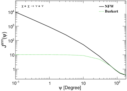
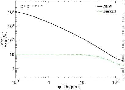
Figure 2: The value of $\mathcal{J}^{ann}(\psi)$ (see Eq. 3) and its average ($\mathcal{J}_{\Delta\Omega}^{ann}(\psi)$) over solid angle $\Delta\Omega$ = $2\pi(1-\cos\psi)$ (see Eq. 5) are shown in left and right panels. In both the panels, black solid and green dashed lines present the corresponding quantities for the NFW and Burkert profiles respectively. We use $\mathcal{J}^{ann}_{\Delta\Omega}(\psi\,=\,180^{\circ})$ for the diffuse dark matter analysis, which has values 3.33 and 1.6 for the NFW and Burkert profiles respectively.

The variation of $\mathcal{J}^{ann}(\psi)$ and $\mathcal{J}_{\Delta\Omega}^{ann}(\psi)$ with angle $\psi$ are shown by the black solid (green dashed) lines in left and right panels of Fig. 2 respectively using the NFW (Burkert) DM halo profile. The value of $\mathcal{J}^{ann}_{\Delta\Omega}$ = 3.33 for the NFW profile and $\mathcal{J}^{ann}_{\Delta\Omega}$ = 1.6 for the Burkert profile with $\Delta\Omega$ = 4$\pi$. The flux of each flavor of $\nu/\bar{\nu}$ per unit energy range per unit solid angle (in units of GeV^-1 sr^-1 cm^-2 s^-1) produced in the final state of dark matter particles annihilation is given by

$$\frac{d^{2}\Phi^{ann}_{\nu/\bar{\nu}}}{{dE}\,d\Omega}=\frac{\langle\sigma_{A}v\rangle}{2}\mathcal{J}^{ann}_{\Delta\Omega}\,\frac{R_{sc}\rho^{2}_{sc}}{4\pi\,m_{\chi}^{2}}\,\,\frac{1}{3}\frac{{dN^{ann}}}{{dE}}\,,$$ (6)

where $\langle\sigma_{A}v\rangle$ is the self-annihilation cross-section in units of cm³ s^-1. The factor $\frac{1}{2}$ is included as we assume the dark matter particle is same as its own antiparticle. The factor $\frac{1}{3}$ takes into account the flavor ratio of $\nu/\bar{\nu}$ on the Earth’s surface. The probability of $\nu_{e}$, $\nu_{\mu}$, and $\nu_{\tau}$ to be produced in the final state are the same. Therefore the flux of $\nu$/$\bar{\nu}$ with each lepton flavor is calculated as the total $\nu$/$\bar{\nu}$ flux divided by the total number of lepton generations, which gives rise to the $\frac{1}{3}$ factor in Eq. 6. The factor 4$\pi$ in the denominator is for the isotropic production of $\nu\bar{\nu}$ in annihilation of dark matter. The parameter $m_{\chi}$ is mass of the DM particles in units of GeV. The energy spectrum of $\nu/\bar{\nu}$ is given by

$$\frac{{dN^{ann}}}{{dE}}=\delta(E_{\nu/\bar{\nu}}-m_{\chi})\,,$$ (7)

since dark matter particles in our galaxy are non-relativistic (local velocity $\sim$ 10^-3c).

2.3 Decay of dark matter

A dark matter particle is assumed to decay into $\nu_{e}+\bar{\nu}_{e}$, $\nu_{\mu}+\bar{\nu}_{\mu}$, and $\nu_{\tau}+\bar{\nu}_{\tau}$ with equal branching ratio:

$$\chi\rightarrow\nu+\bar{\nu}\,.$$ (8)

The $\nu/\bar{\nu}$ flux from dark matter decay is proportional to the line of sight integral of the dark matter distribution, $\mathcal{J}^{dec}(\psi)$, with

$$\mathcal{J}^{dec}(\psi)=\frac{1}{R_{sc}\rho_{sc}}\int_{0}^{l_{max}}dl\,\,\rho\left(\sqrt{R_{sc}^{2}-2lR_{sc}\cos\psi+l^{2}}\right)\,.$$ (9)

The quantity $R_{sc}\rho_{sc}$ in the denominator makes $\mathcal{J}^{dec}(\psi)$ dimensionless. All other symbols have same meaning as before. The quantity $\mathcal{J}_{\Delta\Omega}^{dec}(\psi)$ represents the average value of $\mathcal{J}^{dec}(\psi)$ over the solid angle $\Delta\Omega\,=\,2\pi(1-\cos\psi)$:

$$\mathcal{J}_{\Delta\Omega}^{dec}(\psi)=\frac{1}{2\pi(1-\cos\psi)}\int^{1}_{\cos\psi}2\pi\,{d}(\cos\psi^{\prime})\,\mathcal{J}^{dec}(\psi^{\prime})\,.$$ (10)

Figure 3: Line of sight integral for dark matter decay, $\mathcal{J}^{dec}(\psi)$, (see Eq. 9) vs. $\psi$ and the average value of $\mathcal{J}^{dec}(\psi)$ over solid angle $\Delta\Omega$, i.e., $\mathcal{J}_{\Delta\Omega}^{dec}(\psi)$ (see Eq. 10) for the decay process are shown in left and right panels respectively. In both the panels black solid and green dashed lines present the corresponding quantities for the NFW and the Burkert profiles respectively. We use the value of $\mathcal{J}^{dec}_{\Delta\Omega}$ ($\psi\,=\,180^{\circ}$) in our analysis, which are given by 2.04 and 1.85 for the NFW and Burkert profiles respectively.

For the decaying dark matter, $\mathcal{J}^{dec}(\psi)$ and $\mathcal{J}_{\Delta\Omega}^{dec}(\psi)$ are shown in left and right panels of Fig. 3 respectively by the black solid (green dashed) lines using the NFW (Burkert) profile. We obtain $\mathcal{J}^{dec}_{\Delta\Omega}$( $\psi\,=\,180^{\circ})$ = 2.04 and 1.85 for the NFW and Burkert profile respectively. These agree with those presented in Ref. PalomaresRuiz:2007ry up to uncertainties in the dark matter profile parameters.

The flux of neutrinos of each flavor per unit energy per unit solid angle in units of GeV^-1sr^-1cm^-2 s^-1 from the decay of dark matter particles is given by

$$\frac{d^{2}\Phi^{dec}_{\nu/\bar{\nu}}}{{dE}\,d\Omega}=\mathcal{J}^{dec}_{\Delta\Omega}\,\frac{R_{sc}\rho_{sc}}{4\pi\,m_{\chi}\,\tau}\,\,\frac{1}{3}\frac{{dN^{dec}}}{{dE}}\,,$$ (11)

where $m_{\chi}$ is the mass of DM particle ($\chi$) in GeV, and $\tau$ is the decay lifetime of $\chi$ in second. The factor $\frac{1}{3}$ accounts for the averaging over total number of lepton flavors and 4$\pi$ implies isotropic decay. The mass of dark matter is shared by final $\nu$ and $\bar{\nu}$, thus, their energy spectrum can be written as

$$\frac{{dN^{dec}}}{{dE}}=\delta(E_{\nu/\bar{\nu}}-m_{\chi}/2)\,.$$ (12)

3 Key features of ICAL detector

The proposed 50 kt MagICAL detector INO ; Ahmed:2015jtv is designed to have 151 alternate layers of 5.6 cm thick iron plates (act as target mass) and glass Resistive Plate Chambers (RPCs, act as active detector elements). The plan is to have a modular structure for the detector with a dimension of 48 m (L) $\times$ 16 m (W) $\times$ 14.5 m (H), subdivided into 3 modules, each having a dimension of 16 m $\times$ 16 m $\times$ 14.5 m. The field strength of the magnetized iron plates will be around 1.5 T, with fields greater than 1 T over at least 85$\%$ of the detector volume Behera:2014zca . Bending of charged particles in this magnetic field help us to identify the charges of $\mu^{-}$ and $\mu^{+}$ which are produced in the charged-current (CC) interactions of $\nu_{\mu}$ and $\bar{\nu}_{\mu}$ inside the detector. This magnetic field inside the detector is best suited to observe muons having energies in GeV range, measure their charges, and reconstruct their momentum with high precision Chatterjee:2014vta . The capabilities of ICAL to measure three flavor oscillation parameters based on the information coming from muon energy ($E_{\mu}$) and direction ($\cos\theta_{\mu}$) have already been explored in Refs. Ghosh:2012px ; Thakore:2013xqa . Recently it has been demonstrated that the ICAL detector has ability to detect hadron showers and extract information about hadron energy from them Devi:2013wxa ; Mohan:2014qua . The energy of hadron ($E^{/}_{had}=E_{\nu}-E_{\mu}$) can be calibrated using number of hits in the detector due to hadron showers Devi:2013wxa . In Devi:2014yaa , it has been shown that by adding the hadron energy information ($E^{/}_{had}$) to the muon information ($E_{\mu}$, $\cos\theta_{\mu}$) of each event the sensitivity of ICAL to the neutrino oscillation parameters can be greatly enhanced.

Energy resolution ($\sigma_{E}$) (GeV)	$0.1\,\times$ ($E$/GeV)
Angular resolution ($\Delta\theta$)	$10^{\circ}$
Detection efficiency ($\mathcal{E}$)	$80\%$
CID efficiency ($\mathcal{C}$)	$90\%$

Table 2: The detector characteristics used in the simulations. We use the same detector properties for $\mu^{-}$ and $\mu^{+}$ events.

In this phenomenological study, we explore the physics reach of MagICAL to see the signatures of Galactic diffuse dark matter through neutrino portal using the neutrino energy ($E_{\nu}$) and zenith angle ($\cos\theta_{\nu}$) as reconstructed variables. We consider reconstructed neutrino energy threshold to be 1 GeV for both $\mu^{-}$ and $\mu^{+}$ events. The energy resolution of the MagICAL detector is expected to be quite good, and we assume that the neutrino energy will be reconstructed with a Gaussian energy resolution of 10$\%$ of $E$/GeV (see table 2). As far as the angular resolution is concerned, we use a constant angular resolution of 10^∘. For $\mu^{\mp}$ events, the constant detection efficiency is 80$\%$, and the constant charge identification (CID) efficiency is 90$\%$. The detector properties that we use in our simulation agree quite well with the detector characteristics that have been considered in the existing phenomenological studies related to the MagICAL detector. For example see Refs. Petcov:2005rv ; Blennow:2012gj ; Ghosh:2013zna ; Ghosh:2014dba . We have checked that the representative choices of energy and angular resolutions of $\nu_{\mu}$ and $\bar{\nu}_{\mu}$ that we consider in this work can produce similar results for oscillation studies as obtained by the INO simulation code using muon momentum as variable. In this work, we assume that the 50 kt MagICAL detector will collect atmospheric neutrino data for 10 years giving rise to a total exposure of 500 kt$\cdot$yr.

4 Event spectrum and rates

In this section, we present the expected event spectra and total event rates at the MagICAL detector. To estimate the number of expected $\mu^{-}$ events from atmospheric $\nu_{\mu}$ and $\bar{\nu}_{\mu}$ in the $i$-th energy bin and $j$-th zenith bin at the MagICAL detector, we use the following expression Gandhi:2007td

$$N^{atm}_{ij}(\mu^{-})\,=\,2\pi\,N_{\rm{t}}\,\mathcal{T}\int^{E^{i}_{max}}_{E^{i}_{min}}{dE^{\prime}}\,\int^{\cos\theta^{j}_{max}}_{\cos\theta^{j}_{min}}{d(\cos\theta^{\prime})}\,\int^{1}_{-1}d(\cos\theta)\int^{\infty}_{0}dE\,R({E,E^{\prime}})$$

$$\,R(\theta,\theta^{\prime})\bigg{[}\,\sigma_{\nu_{\mu}}^{CC}({E})\,\mathcal{E}\,\mathcal{C}\,\bigg{\{}\frac{{d^{2}}\Phi_{\nu_{\mu}}}{d\cos\theta\,d{E}}P_{\mu\mu}\,+\,\frac{{d^{2}}\Phi_{\nu_{e}}}{d\cos\theta\,d{E}}P_{e\mu}\bigg{\}}\,+$$

$$\,\bar{\sigma}_{\nu_{\mu}}^{CC}({E})\,\mathcal{\bar{E}}\,(1-\mathcal{\bar{C}})\,\bigg{\{}\frac{{d^{2}}\bar{\Phi}_{\nu_{\mu}}}{d\cos\theta\,d{E}}\bar{P}_{\mu\mu}\,+\,\frac{{d^{2}}\bar{\Phi}_{\nu_{e}}}{d\cos\theta\,d{E}}\bar{P}_{e\mu}\bigg{\}}\bigg{]}.\phantom{11}$$ (13)

In the above equation, $\mathcal{T}$ is the total running time in second, and $N_{t}$ is the total number of target nucleons in the detector. The quantities $E$ ($E^{\prime}$) and $\theta$ ($\theta^{\prime}$) are the true (reconstructed) neutrino energy and zenith angle respectively. For $\mu^{-}$ ($\mu^{+}$) events, $\sigma_{\nu_{\mu}}^{CC}$ ($\bar{\sigma}_{\nu_{\mu}}^{CC}$) is the total neutrino (antineutrino) per nucleon CC cross-section. These cross-sections have been taken from Fig. 9 of Ref. Formaggio:2013kya . We take the unoscillated atmospheric $\nu_{\mu}$ and $\nu_{e}$ fluxes estimated for the INO site in units of m^-2s^-1GeV^-1 sr^-1 from Ref. Honda:2015fha ; HONDA . The probability of a $\nu_{\mu}$ ($\nu_{e}$) to survive (appear) as $\nu_{\mu}$ is denoted by $P_{\mu\mu}$ ($P_{e\mu}$). The parameters $\mathcal{E}$ ($\mathcal{\bar{E}}$) and $\mathcal{C}$ ($\mathcal{\bar{C}}$) are the detection and charge identification efficiencies respectively for $\mu^{-}$ ($\mu^{+}$) events. The quantities $R(E,\,E^{\prime})$ and $R(\theta,\,\theta^{\prime})$ are the Gaussian energy and angular resolution functions of the detector, which are expressed in the following way

$$R(E,\,E^{\prime})=\frac{1}{\sigma_{E}\sqrt{2\pi}}\,\,{\rm{exp}}\,\bigg{\{}\frac{-\,(E^{\prime}-E)^{2}}{2\sigma_{E}^{2}}\bigg{\}},\,$$ (14)

and

$$R(\theta,\,\theta^{\prime})=\frac{1}{\sigma_{\theta}\sqrt{2\pi}}\,\,{\rm{exp}}\,\bigg{\{}\frac{-\,(\cos\theta^{\prime}-\cos\theta)^{2}}{2\sigma_{\theta}^{2}}\bigg{\}}\,.$$ (15)

The parameters $\sigma_{E}$ and $\sigma_{\theta}\,(\sin\theta\,\Delta\theta$) denote the energy and angular resolutions as given in table 2.

Observables	Range	Width	Total bins
Eν (GeV)	$1,15$ $15,25$ $25,50$ $50,100$	1 2 5 10	$\left.\begin{tabular}[]{l}14\\ 5\\ 5\\ 5\end{tabular}\right\}$ 29
$\cos\theta_{\nu}$	$-1,1$	0.5	4

Table 3: The binning scheme adopted for the reconstructed $E_{\nu}$ and $\cos\theta_{\nu}$ for each muon polarity. The last column depicts the total number of bins considered for each observable.

We can estimate the $\mu^{-}$ events in the $i$-th energy bin and $j$-th angular bin from the dark matter induced neutrinos and anitneutrinos by making suitable changes in Eq. 13 in the following fashion

$$N^{dm}_{ij}(\mu^{-})\,=\,2\pi\,N_{\rm{t}}\,\mathcal{T}\int^{E^{i}_{max}}_{E^{i}_{min}}{dE^{\prime}}\,\int^{\cos\theta^{j}_{max}}_{\cos\theta^{j}_{min}}{d(\cos\theta^{\prime})}\int^{1}_{-1}d(\cos\theta)\int^{\infty}_{0}dE\,R({E,E^{\prime}})\,\,R(\theta,\theta^{\prime})\,$$

$$\frac{{d^{2}}\Phi^{dm}}{d\cos\theta\,d{E}}\bigg{[}\,\sigma_{\nu_{\mu}}^{CC}({E})\,\mathcal{E}\,\mathcal{C}\bigg{\{}P_{e\mu}+P_{\mu\mu}+P_{\tau\mu}\bigg{\}}\,+\,\bar{\sigma}_{\nu_{\mu}}^{CC}({E})\,\mathcal{\bar{E}}\,(1-\mathcal{\bar{C}})\,\bigg{\{}\bar{P}_{e\mu}+\bar{P}_{\mu\mu}+\bar{P}_{\tau\mu}\bigg{\}}\bigg{]}.\phantom{111}$$ (16)

In case of dark matter annihilation and decay, we have fluxes of $\nu_{\tau}$ and $\bar{\nu}_{\tau}$ along with the fluxes of $\nu_{e}$, $\bar{\nu}_{e}$, $\nu_{\mu}$, and $\bar{\nu}_{\mu}$. The dark matter induced neutrino and antineutrino fluxes for each flavor are estimated using Eqs. 6 and 11 for annihilation and decay processes respectively. In the above equation, the probability of $\nu_{\tau}$ ($\bar{\nu}_{\tau}$) to appear as $\nu_{\mu}$ ($\bar{\nu}_{\mu}$) at the detector is expressed by $P_{\tau\mu}$ ($\bar{P}_{\tau\mu}$). All the other symbols signify the same parameters as described in Eq. 13. In our analysis, we take $\delta_{\textrm{CP}}$ = 0^∘ and therefore, we can write $P_{\alpha\beta}$ = $P_{\beta\alpha}$ and $\bar{P}_{\alpha\beta}$ = $\bar{P}_{\beta\alpha}$. Due to these properties and unitary nature of the PMNS matrix U Pontecorvo:1957qd ; Maki:1962mu ; Pontecorvo:1967fh , the sums of oscillation probabilities for neutrino and antineutrino in above equation become 1. Therefore, $\nu_{\mu}$ and $\bar{\nu}_{\mu}$ event rates due to the dark matter annihilation/decay do not depend on the values of oscillation parameters.

In our simulation, the full three flavor neutrino oscillation probabilities are incorporated using the PREM profile for the Earth matter density Dziewonski:1981xy . The choices of central values of the oscillation parameters that are used in our simulation lie within the 1$\sigma$ range of these parameters as obtained from the recent global fit studies Forero:2014bxa ; Esteban:2016qun ; Capozzi:2017ipn . We produce all the results in this paper using the following benchmark values of oscillation parameters: $\sin^{2}\theta_{23}$ = 0.5, $\sin^{2}2\theta_{13}$=0.085, $\Delta m_{\textrm{eff}}^{2}$ = $\pm\,2.4\,\times\,10^{-3}$ eV², $\sin^{2}2\theta_{12}$ = 0.84, $\Delta m_{21}^{2}$ = 7.5 $\times$ 10^-5 eV², and $\delta_{\textrm{CP}}$ = 0^∘. The (+) and (-) signs of $\Delta m_{\textrm{eff}}^{2}$ correspond to normal ordering (NO) and inverted ordering (IO) respectively. In fit, we keep the values of oscillation parameters and the choice of mass ordering fixed.

In this analysis, we binned the $\nu$ and $\bar{\nu}$ data separately using reconstructed observables $E_{\nu}$ and $\cos\theta_{\nu}$ as described in table 3. There are total 29 $E_{\nu}$ bins in the range of $E_{\nu}$ = [1, 100] GeV. The bins of $E_{\nu}$ are chosen uneven to ensure that they are consistent with the energy resolution of the detector at various energy ranges. The isotropic nature of the signal allows us to take coarser binning in $\cos\theta_{\nu}$, and we take four $\cos\theta_{\nu}$ bins of equal size in the range [-1, 1]. We use comparatively finer bins for reconstructed E_ν because the signal has a strong dependency on energy of neutrino. We adopt an optimized binning scheme so that we have at least 2 events in each bin. The total number of bins used in our analysis is 29 $\times$ 4 $=$ 116. We show the signal and background event distribution plots as a function of reconstructed neutrino energy for various $\cos\theta_{\nu}$ ranges in section 6 (see Figs. 4 and 6).

5 Simulation method

In our analysis, we consider the dark matter induced neutrinos as signal and treat atmospheric neutrinos as background. If N${}_{ij}^{atm}$ and N${}_{ij}^{dm}$ denote the number of $\mu^{-}$ events produced from the interactions of atmospheric $\nu_{\mu}$ and dark matter induced $\nu_{\mu}$ respectively in the $i$-th energy and $j$-th angular bin (see Eqs. 13 and 16), then the Poissonian $\chi^{2}$ Olive:2016xmw can be written as

$$\chi^{2}(\mu^{-})=\min_{\zeta_{atm},\,\zeta_{dm}}\sum^{N_{E_{\nu}}}_{i=1}\sum^{N_{\cos\theta_{\nu}}}_{j=1}2\bigg{[}N^{th}_{ij}(\mu^{-})-N_{ij}^{exp}(\mu^{-})\,-\,N_{ij}^{exp}(\mu^{-})\ln\frac{N^{th}_{ij}(\mu^{-})}{N^{exp}_{ij}(\mu^{-})}\bigg{]}$$

$$+\,\zeta^{2}_{atm}\,+\,\zeta^{2}_{dm}\,.\phantom{11}$$ (18)

In the above equation, $N_{ij}^{exp}\,=\,N^{atm}_{ij}$ and $N^{th}_{ij}=N^{atm}_{ij}\,(1+\pi_{atm}\,\zeta_{atm})+N^{dm}_{ij}\,(1+\pi_{dm}\,\zeta_{dm})$ neglecting higher order terms. Here, $N_{E_{\nu}}$ = 29 and $N_{\cos\theta_{\nu}}$ = 4 as mentioned in table 3. The quantities $\pi_{dm}$ and $\pi_{atm}$ in Eq. 18 are the over all normalization errors on signal and background respectively. We take $\pi_{dm}$ = $\pi_{atm}$ = 20$\%$. The systematic uncertainties in this analysis are incorporated using the pull method Huber:2002mx ; Fogli:2002au ; GonzalezGarcia:2004wg . The parameters $\zeta_{dm}$ and $\zeta_{atm}$ are the pull variables due to the systematic uncertainties on signal and background respectively. The values of $\zeta_{dm}$ and $\zeta_{atm}$ are obtained by setting $\frac{\partial\chi^{2}}{\partial\zeta_{dm}}$ = 0 and $\frac{\partial\chi^{2}}{\partial\zeta_{atm}}$ = 0, and their values lie within the range -1 to 1. Following the same procedure, $\chi^{2}(\mu^{+})$ for $\mu^{+}$ events is obtained. We calculate the total $\chi^{2}$ by adding the individual contributions from $\mu^{-}$ and $\mu^{+}$ events in the following way

$$\chi^{2}_{\rm{total}}=\chi^{2}(\mu^{-})\,+\,\chi^{2}(\mu^{+})\,.$$ (19)

We notice that our results remain unchanged if we consider larger uncertainties on the atmospheric neutrino events. The reason behind this is that for any choice of $m_{\chi}$ we have many bins in terms of the reconstructed observables E_ν and $\cos\theta_{\nu}$, which are not affected by the dark matter induced neutrinos. Therefore these bins can constrain the uncertainties on the atmospheric neutrino flux. On the other hand, we notice that if we take the larger uncertainties on the dark matter induced neutrino events, say 30$\%$, our final results get modified by 2 to 3$\%$. It is worthwhile to mention that the maximum uncertainty on the signal stems from the dark matter density profile. Therefore, we give our results assuming two different profiles for the dark matter density which are the NFW and the Burkert.

As we have discussed in section 4, the dark matter induced signal does not depend on the oscillation parameters as long as we take the CP-violating phase $\delta_{\rm{CP}}$ = 0^∘. The dependency on the oscillation parameters in the results comes only through the atmospheric neutrino background. We produce all the results assuming normal ordering both in data and theory. We have checked that the results hardly change if we consider inverted ordering. One of the main reasons behind this is that due to our choice of coarser reconstructed $\cos\theta_{\nu}$ bins, the information coming from the MSW effect Mikheev:1986gs ; Mikheev:1986wj ; Wolfenstein:1977ue ; Wolfenstein:1979ni in the atmospheric neutrino events gets smeared out substantially. Another reason is that since the dark matter induced neutrino signal appears only in 2 to 3 $E_{\nu}$ bins (see in Figs. 4 and 6), $\chi^{2}$ is hardly affected due to the change in atmospheric neutrino background in these bins when we switch from NO to IO.

6 Results

6.1 Constraints on annihilation of dark Matter

In this section, we present the constraints on self-annihilation cross-section of dark matter ($\chi\chi\rightarrow\nu\bar{\nu}$) which can be obtained by 500 kt$\cdot$yr of MagICAL exposure. The background consists of conventional atmospheric neutrinos, and the signal consists of neutrinos coming from dark matter annihilation. The simulated event spectra as a function of reconstructed neutrino energy in 500 kt$\cdot$yr exposure of MagICAL detector are presented in Fig. 4. The quantity in the y-axis of Fig. 4 is the number of events per unit energy range multiplied by the mid value in each energy bin. In each panel, the black solid line represents the event distribution of conventional atmospheric $\nu_{\mu}$, denoted by ATM. If DM particles of mass 30 GeV, for example, self-annihilate to $\nu\bar{\nu}$ pairs, then each of these $\nu$ and $\bar{\nu}$ will have 30 GeV of energy. The total neutrino event spectra in MagICAL detector in presence of DM annihilation are shown by the red dotted lines (ATM + DM) in Fig. 4. The value of self-annihilation cross-section of dark matter for these plots is taken to be 3.5 $\times\,10^{-23}$ cm³ s^-1.

$$\begin{array}[]{cc}\includegraphics[width=212.47617pt]{Thenievent-nu-nh-annihil-ct1.pdf}&\includegraphics[width=212.47617pt]{Thenievent-nu-nh-annihil-ct2.pdf}\\ \includegraphics[width=212.47617pt]{Thenievent-nu-nh-annihil-ct3.pdf}&\includegraphics[width=212.47617pt]{Thenievent-nu-nh-annihil-ct4.pdf}\\ \end{array}$$

Figure 4: Event spectra of atmospheric $\nu_{\mu}$ (denoted by ATM) are shown by the black solid lines. The predicted event distributions coming from atmospheric $\nu_{\mu}$ and dark matter originated neutrino (ATM + DM) are shown in red dotted lines for different $\cos\theta$ ranges using 500 kt$\cdot$yr exposure of the MagICAL detector. The signal (DM) is coming from 30 GeV annihilating DM particles here. The mass ordering is taken as NO. The $\chi\chi\rightarrow\nu\bar{\nu}$ cross-section is arbitrarily chosen to $<\sigma v>=3.5\,\times\,10^{-23}$ cm³ s^-1 to have visual clarity.

An excess of $\nu_{\mu}$ events due to dark matter annihilation appears over the ATM around reconstructed neutrino energy of 30 GeV. These events get distributed over nearby energy bins due to the finite energy resolution of the detector. The number of signal and atmospheric events in neutrino mode are 174 and 210 respectively in the energy range [25, 35] GeV and $\cos\theta_{\nu}\in[-1,1]$. There are 4 panels: each represents the event distribution summed over different $\cos\theta_{\nu}$ ranges. The figures in top panels portray the event spectra over $\cos\theta_{\nu}\,\in\,[-1,-0.5]$ and [$-$0.5, 0.0] from left to right. These events are due to upward going neutrinos, which travel a long distance through the Earth matter before they reach the detector. Though in these panels, the signatures of neutrino flavor oscillation are seen in ATM spectra, but the imprints of the Earth matter effect are not visible due to the choice of our large $\cos\theta_{\nu}$ bins. The energy distributions of downward going events are shown in bottom panels from left to right for $\cos\theta_{\nu}$ $\in$ [0.0, 0.5] and [0.5, 1.0] respectively. These neutrinos do not oscillate as they traverse a length smaller than the oscillation wavelength in multi-GeV range. The statistical error bars in these plots associated with different energy bins are equal to the square root of the number of events in the corresponding bins.

Figure 5: (a) The upper limit on self-annihilation cross-section of DM particle ($\chi\chi\rightarrow\nu\bar{\nu}$) at 90$\%$ C.L. (1 d.o.f.) as a function of DM mass $m_{\chi}$ using 500 kt$\cdot$yr exposure of the MagICAL detector. The bound calculated with only $\nu_{\mu}$ ($\bar{\nu}_{\mu}$)-induced events is shown with red dashed (blue dot-dashed) line as MagICAL can distinguish $\nu_{\mu}$ from $\bar{\nu}_{\mu}$. The upper bound obtained by combining these two channels is also shown by the black solid line in the figure. We take the NFW as DM profile. (b) The upper bounds on the self-annihilation cross-section ($\chi\chi\rightarrow\nu\bar{\nu}$) of dark matter are presented for the NFW (black solid) and Burkert (green dashed) profiles combining the information coming from $\nu_{\mu}$ and $\bar{\nu}_{\mu}$. For both (a) and (b), the choice of mass ordering is NO.

The charge identification ability of the MagICAL detector provides an opportunity to explore the same physics in neutrino and antineutrino channels separately. This is not possible in water Cherenkov, liquid scintillator, and liquid argon based detectors. The MagICAL detector will have separate data sets for $\nu_{\mu}$ and $\bar{\nu}_{\mu}$. The total sensitivity is obtained by combining the $\nu_{\mu}$ and $\bar{\nu}_{\mu}$ data sets according to Eq. 19. We present results by using $\nu_{\mu}$ and $\bar{\nu}_{\mu}$ data separately, and then combining these two. The upper limits on self-annihilation cross-section ($\langle\sigma v\rangle$) of DM particles for the process $\chi\chi\rightarrow\nu\bar{\nu}$ at 90$\%$ C.L. (1 d.o.f.) that MagICAL will obtain with 10 years of data are represented in Fig. 5. The red dashed, blue dot-dashed, and the black solid lines in Fig. 5(a) represent the limits on $\langle\sigma v\rangle$ from $\nu_{\mu}$, $\bar{\nu}_{\mu}$, and the combination of $\nu_{\mu}$ and $\bar{\nu}_{\mu}$ data respectively using the NFW profile. Analysis with $\nu_{\mu}$ gives tighter bound than $\bar{\nu}_{\mu}$ because of the higher statistics of $\nu_{\mu}$ over $\bar{\nu}_{\mu}$.

At higher energies, the atmospheric neutrino flux (background) decreases, and same happens to the signal coming from dark matter self annihilation because of its $m^{-2}_{\chi}$ dependence (see Eq. 6). A competition between these two effects lowers the signal to background ratio for heavy dark matter particles. Thus, the bound on $\langle\sigma v\rangle$ becomes weaker for heavy DM. We can have a rough estimate of how $\langle\sigma v\rangle$ depends on $m_{\chi}$ in the range say 4 to 8 GeV by mainly considering the energy dependence of flux and interaction cross-section in both signal and background. In this $m_{\chi}$ range which also corresponds to neutrino energy range of 4 to 8 GeV, the atmospheric flux varies as $\sim E_{\nu}^{-2.7}$, whereas neutrinos flux from the annihilating DM goes as $\langle\sigma v\rangle/m_{\chi}^{2}$. For both signal and background, the neutrino-nucleon CC cross-section is approximately proportional to $E_{\nu}$ or $m_{\chi}$ in case of annihilation. Therefore, the neutrino signal from dark matter annihilation ($S$) depends on $m_{\chi}$ in the following way: $S\,\propto\frac{\langle\sigma v\rangle}{m_{\chi}^{2}}\cdot m_{\chi}\,=\,\langle\sigma v\rangle/{m_{\chi}}$. As far as background ($B$) is concerned, $B\propto m_{\chi}^{-2.7}\cdot m_{\chi}\,=\,m_{\chi}^{-1.7}$. Hence, in case of annihilation, $S/\sqrt{B}\propto\langle\sigma v\rangle\cdot m_{\chi}^{-0.15}$ or, $\langle\sigma v\rangle\propto m_{\chi}^{0.15}$ if $S/\sqrt{B}$ remains constant. From Fig. 5(a), we can see that at $m_{\chi}$ = 4 GeV, the limit on $\langle\sigma v\rangle$ is 1.2 $\times$ 10^-24 cm³ s^-1 in case of $\nu+\bar{\nu}$ modes. Now, from our approximate expression as mentioned above, the limit on $\langle\sigma v\rangle$ at $m_{\chi}$ = 8 GeV should be around 1.2$\,\times\,$10${}^{-24}\,\times\,(8/4)^{0.15}$ cm³ s^-1 = $1.33\,\times\,10^{-24}$ cm³ s^-1, which is indeed the case as can be seen from the black solid line in Fig. 5(a). If we want to do the same exercise for $m_{\chi}<$ 4 GeV, then the only change that we have to make is that the atmospheric neutrino flux varies as $E_{\nu}^{-2}$ at those energies instead of $E_{\nu}^{-2.7}$. On the other hand, to explain the nature of the same curve for $m_{\chi}$ above 8 GeV, we have to also take into account the effect of neutrino flavor oscillation and detector response which have nontrivial dependence on $E_{\nu}$ whereas, the atmospheric neutrino flux still varies as $E_{\nu}^{-2.7}$ in this energy range.

We compare the constraints with the NFW and the Burkert profiles by black solid and green dashed lines respectively in Fig. 5(b) combining the neutrino and antineutrino data. We obtain better sensitivity with the NFW profile than with the Burkert profile. The average value of $\mathcal{J}$ factor over 4$\pi$ solid angle for the Burkert profile is smaller than that for the NFW profile. Thus, the signal strength with Burkert profile is smaller than that with the NFW profile. We have $\mathcal{J}^{ann}_{\Delta\Omega}$ = 3.33 and 1.60 for the NFW and Burkert profiles respectively, with $\Delta\Omega$ = 4$\pi$.

6.2 Constraints on decay of dark matter

Assuming that dark matter particles have a mass of 30 GeV, and they decay to $\nu\bar{\nu}$ pairs, then the energy that each $\nu$ and $\bar{\nu}$ carries is 15 GeV. These events give rise to an excess of $\nu_{\mu}$ and $\bar{\nu}_{\mu}$ events around reconstructed neutrino energy of 15 GeV on top of the atmospheric neutrino event distribution as shown in Fig. 6. The black solid lines represent the event distributions for the atmospheric neutrinos and the red dotted lines show event distributions for background along with the signal. The four panels in Fig. 6 correspond to different $\cos\theta_{\nu}$ ranges as mentioned in the figure legends. Here, we assume the lifetime ($\tau$) of dark matter to be 4.7 $\times\,10^{24}$ s and we take 500 kt$\cdot$yr exposure for the MagICAL detector. We can see from Fig. 6 that the events due to the decay of dark matter get distributed around 15 GeV due to the finite energy resolution of detector. In this case, the number of the signal and background events are 81 and 289 respectively in the reconstructed energy range [13, 17] GeV and $\cos\theta_{\nu}\in[-1,1]$.

$$\begin{array}[]{cc}\includegraphics[angle={0.0},width=212.47617pt]{Thenievent-nu-nh-decay-ct1.pdf}&\includegraphics[angle={0.0},width=212.47617pt]{Thenievent-nu-nh-decay-ct2.pdf}\\ \includegraphics[angle={0.0},width=212.47617pt]{Thenievent-nu-nh-decay-ct3.pdf}&\includegraphics[angle={0.0},width=212.47617pt]{Thenievent-nu-nh-decay-ct4.pdf}\\ \end{array}$$

Figure 6: The event distribution of atmospheric $\nu_{\mu}$ (denoted as ATM) and the predicted $\nu_{\mu}$ event spectra in presence of decay of 30 GeV dark matter particles (denoted as ATM + DM) in different $\cos\theta_{\nu}$ ranges using 500 kt$\cdot$yr exposure of the MagICAL detector. Black solid (red dotted) line represents the ATM (ATM + DM). The mass ordering is taken as NO. The lifetime of dark matter is arbitrarily chosen (4.7 $\times\,10^{24}$ s) for sake of visual clarity.

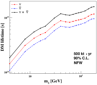
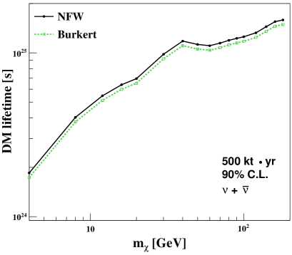
Figure 7: (a) The lower bound on the decay lifetime of dark matter ($\chi\rightarrow\nu\bar{\nu}$) as a function of DM mass $m_{\chi}$ at 90$\%$ C.L. (1 d.o.f.) obtained using only $\nu_{\mu}$ and only $\bar{\nu}_{\mu}$ data using 500 kt$\cdot$yr exposure of MagICAL. The red dashed (blue dot-dashed) line shows the sensitivity coming from $\nu_{\mu}$ ($\bar{\nu}_{\mu}$)-induced events. The black solid line represents the same combining $\nu_{\mu}$ and $\bar{\nu}_{\mu}$ events at $\chi^{2}$ level. We take NO as mass ordering. (b) The constraints on the decay lifetime of dark matter ($\chi\rightarrow\nu\bar{\nu}$) assuming the NFW (black solid line) and Burkert (green dashed line) profiles using 500 kt$\cdot$yr of MagICAL exposure. Here the results are shown combining $\nu$ and $\bar{\nu}$ (see section 5 for detail).

The future sensitivity of the MagICAL detector to set a lower limit on the lifetime ($\tau$) of dark matter as a function of $m_{\chi}$ is shown in Fig. 7. We give the results at 90$\%$ C.L. (1 d.o.f.) assuming 500 kt$\cdot$yr exposure of the proposed MagICAL detector. Here, we assume the dark matter density profile to be the NFW. The red dashed (blue dot-dashed) line in Fig. 7(a) represents the bound which we obtain using $\nu_{\mu}$ ($\bar{\nu}_{\mu}$) data set. The bound gets improved when we add the $\nu_{\mu}$ and $\bar{\nu}_{\mu}$ data sets and the corresponding result is shown by the black solid line. Here, we see that the limits on the dark matter lifetime get improved when we consider higher m_χ. It happens for the following reasons. The flux of neutrinos coming from the dark matter decay (signal) has a $m_{\chi}^{-1}$ dependence (see Eq. 11) and the atmospheric neutrino flux (background) gets reduced substantially at higher energies. We find that in presence of these two competing effects, ultimately, the signal over background ratio gets improved for higher $m_{\chi}$, which allows us to place restrictive bounds on the lifetime of dark matter. In Fig. 7(a), we can explain how the limit on dark matter life time $\tau$ depends on $m_{\chi}$ in the range say 8 GeV $\leq$ $m\chi$ $\leq$ 16 GeV by mainly taking into account the energy dependence of the flux and neutrino-nucleon CC cross-section in the same fashion which adopt to explain the bound on $\langle\sigma v\rangle$ in the previous section. The above range of $m_{\chi}$ corresponds to the $E_{\nu}$ range of 4 GeV to 8 GeV, since the neutrino energy from decaying DM is $E_{\nu}=m_{\chi}/2$. Here, the neutrino flux from decaying DM is proportional to $\frac{1}{m_{\chi}\tau}$ (see Eq. 11). Thus, the neutrino signal ($S$) from dark matter decay varies as $S\propto\frac{1}{m_{\chi}\tau}\cdot m_{\chi}=1/\tau$, while the background varies with $m_{\chi}$ in the same way as we see in case of annihilation which is $B\propto\,m_{\chi}^{-1.7}$. Hence, in case of decaying DM, $S/\sqrt{B}\propto\frac{1}{\tau}\cdot m_{\chi}^{0.85}$  or, $\tau\propto m_{\chi}^{0.85}$ for a fixed value of $S/\sqrt{B}$. From Fig 7(a), it can be seen that at $m_{\chi}$ = 8 GeV, the limit on $\tau$ is 4.0$\,\times\,$10²⁴ s combining $\nu$ and $\bar{\nu}$ modes. From the simple $m_{\chi}$ dependence of $\tau$ that we discuss above, at 16 GeV, the limit on $\tau$ should be around $4.0\,\times\,10^{24}\,\times\,(16/8)^{0.85}\,\textrm{s}\,=\,7.21\,\times\,10^{24}\,\textrm{s}$, which is very close to the value as can be seen from the black solid line in Fig 7(a). To obtain the similar analytical understanding for $m_{\chi}$ below 8 GeV, we need to make suitable changes in the energy dependence of atmospheric neutrino flux which we have already discussed in the previous section. Similarly, to see how $\tau$ varies with $m_{\chi}$ above 16 GeV, we have to also take into account the nontrivial energy dependence of neutrino flavor conversion and detector response along with flux and cross-section.

Due to the uncertainties in the dark matter density profiles, we present the bound on decay lifetime of dark matter with the profiles: NFW and Burkert by the black solid and green dashed line respectively in Fig. 7(b). Ref. Dash:2014sza considers only $\mu^{+}\mu^{-}$ as final states for dark matter decay in the context of ICAL-INO, although their constraints are much weaker.

6.3 Comparison with other experiments

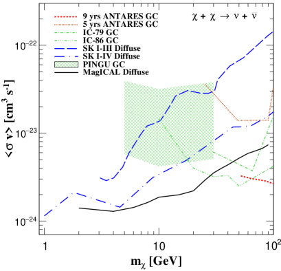
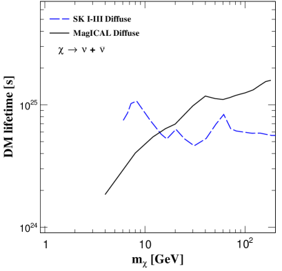
Figure 8: (a) Current bounds at 90$\%$ C.L. (1 d.o.f.) on self-annihilation cross-section which are obtained from the first three phases of Super-Kamiokande Mijakowski:2011zz (blue long-dashed line), the four phases of Super-Kamiokande Mijakowski:2016cph (blue long-dash-dotted line), IceCube Aartsen:2015xej ; Aartsen:2017ulx (green dot-dashed and green triple-dot-dashed lines), and ANTARES Adrian-Martinez:2015wey ; Albert:2016emp (red dotted and red dashed lines) are shown. The future sensitivity of PINGU Aartsen:2014oha with its 1 year of exposure is shown by green shaded region. We compare these limits with the bound obtained from 500 kt$\cdot$yr MagICAL (black solid line) detector. For all the cases the NFW profile is used. (b) Blue long-dashed line shows the current bound on decay lifetime of DM from the first three phases of Super-Kamiokande Mijakowski:2011zz using the NFW profile. We compare this limit with the performance of 500 kt$\cdot$yr MagICAL detector (black solid line) using the same NFW profile.

Various experiments present the bounds on the self-annihilation cross-section of $\chi\chi\rightarrow\nu\bar{\nu}$ and the decay lifetime of $\chi\rightarrow\nu\bar{\nu}$ processes. Fig. 8(a) shows a comparison of the current bounds on $\langle\sigma v\rangle$ at 90$\%$ C.L. (1 d.o.f.) from the first three phases of the Super-Kamiokande Mijakowski:2011zz (blue long-dashed line), the four phases of the Super-Kamiokande Mijakowski:2016cph (blue long-dash-dotted line), IceCube Aartsen:2015xej ; Aartsen:2017ulx (green dot-dashed and green triple-dot-dashed lines), ANTARES Adrian-Martinez:2015wey ; Albert:2016emp (red dotted and red dashed lines), PINGU Aartsen:2014oha (green shade), and from the MagICAL detector (black solid line) for the process $\chi\chi\rightarrow\nu\bar{\nu}$. We do not show the weaker limits from Baikal NT200 Avrorin:2016yhw . In Fig. 8(b), we compare the limits on decay lifetime ($\tau$) for the process $\chi\rightarrow\nu\bar{\nu}$ from the first three phases of the Super-Kamiokande experiment Mijakowski:2011zz (blue long-dashed line) and the present work (black solid line).

Due to the lower energy threshold of MagICAL, the dark matter constraints can be estimated for $m_{\chi}$ values which are as low as 2 GeV and 4 GeV in case of annihilating and decaying dark matter respectively. The good energy and direction resolutions of MagICAL detector help to strongly constrain the $\langle\sigma v\rangle$ and $\tau$ for $m_{\chi}$ in multi-GeV range. The constraints on $\langle\sigma v\rangle$ obtained using 319.7 live-days of data from IceCube operating in its 79 string configuration during 2010 and 2011 are stronger than MagICAL for dark matter masses heavier than $\sim$ 50 GeV (see green dot-dashed line in Fig. 8(a)) Abbasi:2011eq ; Dasgupta:2012bd ; Aartsen:2013dxa ; Aartsen:2014hva ; Moline:2014xua ; Rott:2014kfa ; Aisati:2015vma ; Aartsen:2015xej ; Chianese:2016opp ; Boucenna:2015tra ; Aisati:2015ova ; Aartsen:2016pfc . But, if we consider the limits on $\langle\sigma v\rangle$ estimated using three years of the IceCube/DeepCore data Aartsen:2017ulx , then their performance becomes better than the MagICAL detector for $m_{\chi}\geq 30$ GeV (see green triple-dot-dashed line in Fig. 8(a)). Using the 9 years data of ANTARES, no excess was found over the expected neutrino events in the range of WIMP mass 50 GeV $\leq m_{\chi}\leq$ 100 GeV, and they presented the most stringent constraint on $\langle\sigma v\rangle$ for $m_{\chi}\geq$ 70 GeV Albert:2016emp . However, for dark matter masses $\lesssim$ 100 GeV, the potential constraints from MagICAL are comparable or slightly better than that from Super-Kamiokande Mijakowski:2011zz ; Mijakowski:2016cph . The limit on $\langle\sigma v\rangle$ by 500 kt$\cdot$yr exposure of MagICAL detector is better than that from 1 year exposure of PINGU Aartsen:2014oha . The constraints on dark matter annihilation and decay that we show in Fig. 8 can only be obtained from neutrino telescopes, including liquid scintillator detectors Kumar:2015nja ; Wurm:2011zn . The dark matter masses that we consider are too low for efficient electroweak bremsstrahlung, and hence gamma-ray constraints on this channel are weak Kachelriess:2007aj ; Bell:2008ey ; Bell:2011eu ; Bell:2011if ; Cirelli:2010xx ; Murase:2015gea ; Esmaili:2015xpa ; Chowdhury:2016bxs ; Queiroz:2016zwd . Since MagICAL can distinguish between $\mu^{+}$ and $\mu^{-}$, it can also give constraints on exotic lepton number violating dark matter interactions. The potential dark matter constraints from Baikal-GVD, and Hyper-Kamiokande will be stronger or comparable Avrorin:2014vca ; Abe:2011ts . The complementarity of INO-MagICAL with PINGU and Hyper-Kamiokande will certainly make dark matter physics richer.

6.4 The constraints on DM-induced neutrino flux

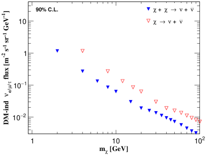
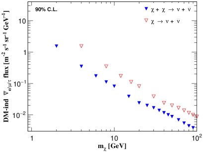
Figure 9: The limit on (a) $\nu_{e/\mu/\tau}$ and (b) $\bar{\nu}_{e/\mu/\tau}$ flux produced from the dark matter in Milky Way galaxy at 90$\%$ C.L. (1 d.o.f.) by 500 kt$\cdot$yr MagICAL detector. The blue filled and red empty triangles are for the annihilation and decay of dark matter particles respectively.

We can use the constraints on $\langle\sigma v\rangle$ (see section 6.1) and $\tau$ (see section 6.2) in Eqs. 6 and 11 respectively to place the upper bound on the neutrino and antineutrino flux from dark matter . In Fig. 9(a), the blue filled triangles and red empty triangles depict the upper bounds on $\nu_{e}/\nu_{\mu}/\nu_{\tau}$ flux at 90$\%$ C.L. (1 d.o.f.) using the constraints on $\langle\sigma v\rangle$ (in case of annihilation) and $\tau$ (in case of decay) respectively. Fig. 9(b) shows the same for $\bar{\nu}_{e}/\bar{\nu}_{\mu}/\bar{\nu}_{\tau}$ flux. The mass ordering is taken as NO and the dark matter profile is assumed to be NFW. We can see from both the panels in Fig. 9 that the limits on neutrino (left panel) and antineutrino (right panel) flux from both annihilation and decay improve as we increase the value of $m_{\chi}$. We can understand this behavior in the following way. We know that the atmospheric neutrino event rates which serve as background for annihilation and decay decrease as we go to higher neutrino energy. This can be clearly seen from Fig. 4 and also Fig. 6. This is also true for atmospheric antineutrino events. Since, the atmospheric neutrino and antineutrino backgrounds get reduced when we go from lower to higher $m_{\chi}$, we need less dark matter induced neutrino and antineutrino flux for both annihilation and decay to obtain the same confidence level in $\Delta\chi^{2}$ which is 2.71 at 90$\%$ C.L. (1 d.o.f). Hence, we can place better constraints on the DM induced neutrino and anitneutrino flux as we move from lower to higher $m_{\chi}$ values. Another feature that is emerging from both the panels in Fig. 9 that we have better constraints on the neutrino and antineutrino flux obtained from the annihilation of dark matter as compare to its decay for a fixed $m_{\chi}$. We can also explain this feature in the following way. For a fixed value of $m_{\chi}$, the available energy of neutrino and antineutrino, $E_{\nu/\bar{\nu}}$, is equal to $m_{\chi}$ for annihilation and $m_{\chi}$/2 for decay. Let us consider the case for $m_{\chi}\,=\,10$ GeV in both the panels. In this case, the available neutrino/antineutrino energy for annihilation (decay) is 10 GeV (5 GeV). Now, we already know that the background events induced by atmospheric neutrino and anitneutrino flux are higher at 5 GeV (in case of decay) as compared to 10 GeV (in case of annihilation). Therefore, for a fixed choice of $m_{\chi}$ value, we need higher neutrino and antineutrino flux from decaying DM as compare to annihilating DM to place the constraints at same confidence level.

7 Conclusions

We explore the prospects of detecting diffuse dark matter in the Milky Way galaxy at the proposed INO-MagICAL detector. The future sensitivity of 500 kt$\cdot$yr MagICAL detector to constrain the dark matter self-annihilation cross-section ($\langle\sigma v\rangle$) and decay lifetime ($\tau$) for $\chi\chi\rightarrow\nu\bar{\nu}$ and $\chi\rightarrow\nu\bar{\nu}$ processes respectively are estimated. We find that MagICAL will be able to probe new parameter space for low mass dark matter.

Combining information from $\nu$ and $\bar{\nu}$ modes, the future limits on $\langle\sigma v\rangle$ and $\tau$ are $\leq$ 1.87 $\times\,10^{-24}$ cm³ s^-1 and $\geq$ 4.8 $\times\,10^{24}$ s respectively at 90$\%$ C.L. (1 d.o.f.) for $m_{\chi}$ = 10 GeV assuming the NFW profile. These limits will be novel and they will address many viable dark matter models. The limits for higher dark matter masses will also be competitive with other neutrino telescopes.

We have also shown the bounds on $\langle\sigma v\rangle$ and $\tau$ with $\nu$ and $\bar{\nu}$ data separately. This enables us to probe the same physics through the $\nu$ and $\bar{\nu}$ channels due to the charge identification capability of the MagICAL detector.

Although, we have studied the processes $\chi\chi\rightarrow\nu\bar{\nu}$ and $\chi\rightarrow\nu\bar{\nu}$, other final states like $\mu^{+}\mu^{-}$, $\tau^{+}\tau^{-}$, $b\bar{b}$ are also possible. The constraints on these channels obtained from the gamma-ray detectors are much stronger, and hence we do not consider them. Since the analysis is done for the diffuse dark matter component of the Milky Way galaxy, the constraints on self-annihilation cross-section and decay lifetime are robust and conservative, and the constraints have mild dependence on the dark matter profile. Besides new and novel methods in dark matter indirect detection physics Speckhard:2015eva ; Powell:2016zbo , it is imperative that we fully utilize the capabilities of new and upcoming detectors. Our work explores the capabilities of INO-MagICAL to search for dark matter, and we encourage the community to look into this signature in more detail.

8 Acknowledgment

A.K. would like to thank the INO project for financial support. R.L. thanks KIPAC for financial help. S.K.A. is supported by DST/INSPIRE Research Grant No. IFA-PH-12, Department of Science and Technology, India. We thank Amol Dighe, Pankaj Agrawal, Ajit Srivastava, and Tarak Thakore for useful discussions.

Appendix A Oscillation of DM induced neutrinos

The oscillation probability of neutrino from one flavor ($\alpha$) to another flavor ($\beta$) in vacuum is given by

$$P_{\alpha\beta} =\sum_{k=l=1}^{3}\,|U_{\alpha k}|^{2}\,|\,U_{\beta l}|^{2}\,$$

$$+\,2\,\sum_{l>k}\,Re(\,U_{\alpha k}\,U^{*}_{\beta k}\,U^{*}_{\alpha l}\,U_{\beta l})\,\cos(\Delta E_{lk}\,L)$$

$$-\,2\,\sum_{l>k}\,Re(\,U_{\alpha k}\,U^{*}_{\beta k}\,U^{*}_{\alpha l}\,U_{\beta l})\,\sin(\Delta E_{lk}\,L)\,,$$ (20)

where U as the 3 $\times$ 3 unitary PMNS matrix Pontecorvo:1957qd ; Maki:1962mu ; Pontecorvo:1967fh . When $L$ is very large, 2nd and 3rd terms in Eq. 20 get averaged out to zero due to very rapid oscillations, and give rise to the following expression

$$P_{\alpha\beta}=\sum_{k=1}^{3}\,|U_{\alpha k}|^{2}\,|\,U_{\beta k}|^{2}\,.$$ (21)

We assume that the annihilation/decay of dark matter particles produce $\nu_{e}$, $\nu_{\mu}$, and $\nu_{\tau}$ in the ratio of 1:1:1 at the source. During their propagation through the astronomical distance from source to detector, they undergo vacuum oscillation. Imposing the unitary property of U in Eq. 21, the ratio of neutrino flavors at the Earth surface remains 1:1:1, and this is true irrespective of the values of oscillation parameters.

References

- (1) Planck Collaboration, P. A. R. Ade et al., Planck 2015 results. XIII. Cosmological parameters, arXiv:1502.01589.
- (2) F. Zwicky, Die Rotverschiebung von extragalaktischen Nebeln, Helv. Phys. Acta 6 (1933) 110–127.
- (3) V. C. Rubin and W. K. Ford, Jr., Rotation of the Andromeda Nebula from a Spectroscopic Survey of Emission Regions, Astrophys. J. 159 (1970) 379–403.
- (4) L. E. Strigari, Galactic Searches for Dark Matter, Phys. Rept. 531 (2013) 1–88, [arXiv:1211.7090].
- (5) D. Clowe, M. Bradac, A. H. Gonzalez, M. Markevitch, S. W. Randall, C. Jones, and D. Zaritsky, A direct empirical proof of the existence of dark matter, Astrophys. J. 648 (2006) L109–L113, [astro-ph/0608407].
- (6) WMAP Science Team Collaboration, E. Komatsu et al., Results from the Wilkinson Microwave Anisotropy Probe, PTEP 2014 (2014) 06B102, [arXiv:1404.5415].
- (7) G. Steigman, Neutrinos And Big Bang Nucleosynthesis, Adv. High Energy Phys. 2012 (2012) 268321, [arXiv:1208.0032].
- (8) G. Jungman, M. Kamionkowski, and K. Griest, Supersymmetric dark matter, Phys. Rept. 267 (1996) 195–373, [hep-ph/9506380].
- (9) G. Bertone, D. Hooper, and J. Silk, Particle dark matter: Evidence, candidates and constraints, Phys. Rept. 405 (2005) 279–390, [hep-ph/0404175].
- (10) L. Bergström, Nonbaryonic dark matter: Observational evidence and detection methods, Rept. Prog. Phys. 63 (2000) 793, [hep-ph/0002126].
- (11) J. Ellis and K. A. Olive, Supersymmetric Dark Matter Candidates, arXiv:1001.3651.
- (12) DAMA, LIBRA Collaboration, R. Bernabei et al., New results from DAMA/LIBRA, Eur. Phys. J. C67 (2010) 39–49, [arXiv:1002.1028].
- (13) LUX Collaboration, D. S. Akerib et al., Improved Limits on Scattering of Weakly Interacting Massive Particles from Reanalysis of 2013 LUX Data, Phys. Rev. Lett. 116 (2016), no. 16 161301, [arXiv:1512.03506].
- (14) SuperCDMS Collaboration, R. Agnese et al., New Results from the Search for Low-Mass Weakly Interacting Massive Particles with the CDMS Low Ionization Threshold Experiment, Phys. Rev. Lett. 116 (2016), no. 7 071301, [arXiv:1509.02448].
- (15) XENON100 Collaboration, E. Aprile et al., Dark Matter Results from 225 Live Days of XENON100 Data, Phys. Rev. Lett. 109 (2012) 181301, [arXiv:1207.5988].
- (16) DarkSide Collaboration, P. Agnes et al., Results from the first use of low radioactivity argon in a dark matter search, Phys. Rev. D93 (2016), no. 8 081101, [arXiv:1510.00702].
- (17) PandaX Collaboration, X. Xiao et al., Low-mass dark matter search results from full exposure of the PandaX-I experiment, Phys. Rev. D92 (2015), no. 5 052004, [arXiv:1505.00771].
- (18) M. Lindner, A. Merle, and V. Niro, Enhancing Dark Matter Annihilation into Neutrinos, Phys. Rev. D82 (2010) 123529, [arXiv:1005.3116].
- (19) S. K. Agarwalla, M. Blennow, E. Fernandez Martinez, and O. Mena, Neutrino Probes of the Nature of Light Dark Matter, JCAP 1109 (2011) 004, [arXiv:1105.4077].
- (20) Y. Farzan, Flavoring Monochromatic Neutrino Flux from Dark Matter Annihilation, JHEP 02 (2012) 091, [arXiv:1111.1063].
- (21) P. Mijakowski, Direct and Indirect Search for Dark Matter. PhD thesis, Warsaw, Inst. Nucl. Studies, 2011.
- (22) M. Blennow, M. Carrigan, and E. Fernandez Martinez, Probing the Dark Matter mass and nature with neutrinos, JCAP 1306 (2013) 038, [arXiv:1303.4530].
- (23) M. Gustafsson, T. Hambye, and T. Scarna, Effective Theory of Dark Matter Decay into Monochromatic Photons and its Implications: Constraints from Associated Cosmic-Ray Emission, Phys. Lett. B724 (2013) 288–295, [arXiv:1303.4423].
- (24) C. El Aisati, M. Gustafsson, T. Hambye, and T. Scarna, Dark Matter Decay to a Photon and a Neutrino: the Double Monochromatic Smoking Gun Scenario, Phys. Rev. D93 (2016), no. 4 043535, [arXiv:1510.05008].
- (25) L. A. Anchordoqui, V. Barger, H. Goldberg, X. Huang, D. Marfatia, L. H. M. da Silva, and T. J. Weiler, IceCube neutrinos, decaying dark matter, and the Hubble constant, Phys. Rev. D92 (2015), no. 6 061301, [arXiv:1506.08788].
- (26) C. Arina, S. Kulkarni, and J. Silk, Monochromatic neutrino lines from sneutrino dark matter, Phys. Rev. D92 (2015), no. 8 083519, [arXiv:1506.08202].
- (27) V. Gonzalez Macias and J. Wudka, Effective theories for Dark Matter interactions and the neutrino portal paradigm, JHEP 07 (2015) 161, [arXiv:1506.03825].
- (28) V. Gonzalez-Macías, J. I. Illana, and J. Wudka, A realistic model for Dark Matter interactions in the neutrino portal paradigm, JHEP 05 (2016) 171, [arXiv:1601.05051].
- (29) J. D. Zornoza, Indirect search for dark matter with neutrino telescopes, arXiv:1601.05691.
- (30) C. Garcia-Cely and J. Heeck, Neutrino Lines from Majoron Dark Matter, arXiv:1701.07209.
- (31) J. F. Beacom, N. F. Bell, and G. D. Mack, General Upper Bound on the Dark Matter Total Annihilation Cross Section, Phys. Rev. Lett. 99 (2007) 231301, [astro-ph/0608090].
- (32) H. Yuksel, S. Horiuchi, J. F. Beacom, and S. Ando, Neutrino Constraints on the Dark Matter Total Annihilation Cross Section, Phys. Rev. D76 (2007) 123506, [arXiv:0707.0196].
- (33) Fermi-LAT Collaboration, M. Ackermann et al., Updated search for spectral lines from Galactic dark matter interactions with pass 8 data from the Fermi Large Area Telescope, Phys. Rev. D91 (2015), no. 12 122002, [arXiv:1506.00013].
- (34) R. Laha, K. C. Y. Ng, B. Dasgupta, and S. Horiuchi, Galactic center radio constraints on gamma-ray lines from dark matter annihilation, Phys. Rev. D87 (2013), no. 4 043516, [arXiv:1208.5488].
- (35) CMS Collaboration, V. Khachatryan et al., Search for dark matter and unparticles produced in association with a Z boson in proton-proton collisions at 8 TeV, Phys. Rev. D93 (2016), no. 5 052011, [arXiv:1511.09375].
- (36) CMS Collaboration, S. Chatrchyan et al., Search for Dark Matter and Large Extra Dimensions in pp Collisions Yielding a Photon and Missing Transverse Energy, Phys. Rev. Lett. 108 (2012) 261803, [arXiv:1204.0821].
- (37) ATLAS Collaboration, G. Aad et al., Search for dark matter candidates and large extra dimensions in events with a photon and missing transverse momentum in collision data at TeV with the ATLAS detector, Phys. Rev. Lett. 110 (2013), no. 1 011802, [arXiv:1209.4625].
- (38) A. Ghosh, T. Thakore, and S. Choubey, Determining the Neutrino Mass Hierarchy with INO, T2K, NOvA and Reactor Experiments, JHEP 04 (2013) 009, [arXiv:1212.1305].
- (39) M. M. Devi, T. Thakore, S. K. Agarwalla, and A. Dighe, Enhancing sensitivity to neutrino parameters at INO combining muon and hadron information, JHEP 10 (2014) 189, [arXiv:1406.3689].
- (40) ICAL Collaboration, S. Ahmed et al., Physics Potential of the ICAL detector at the India-based Neutrino Observatory (INO), arXiv:1505.07380.
- (41) L. S. Mohan and D. Indumathi, Simulations study of neutrino oscillation parameters with the Iron Calorimeter Detector (ICAL): an improved analysis, arXiv:1605.04185.
- (42) T. Thakore, A. Ghosh, S. Choubey, and A. Dighe, The Reach of INO for Atmospheric Neutrino Oscillation Parameters, JHEP 05 (2013) 058, [arXiv:1303.2534].
- (43) D. Kaur, M. Naimuddin, and S. Kumar, The sensitivity of the ICAL detector at India-based Neutrino Observatory to neutrino oscillation parameters, Eur. Phys. J. C75 (2015), no. 4 156, [arXiv:1409.2231].
- (44) N. Dash, V. M. Datar, and G. Majumder, Sensitivity of the INO-ICAL detector to magnetic monopoles, Astropart. Phys. 70 (2015) 33–38, [arXiv:1406.3938].
- (45) A. Chatterjee, R. Gandhi, and J. Singh, Probing Lorentz and CPT Violation in a Magnetized Iron Detector using Atmospheric Neutrinos, JHEP 06 (2014) 045, [arXiv:1402.6265].
- (46) A. Chatterjee, P. Mehta, D. Choudhury, and R. Gandhi, Testing nonstandard neutrino matter interactions in atmospheric neutrino propagation, Phys. Rev. D93 (2016), no. 9 093017, [arXiv:1409.8472].
- (47) S. Choubey, A. Ghosh, T. Ohlsson, and D. Tiwari, Neutrino Physics with Non-Standard Interactions at INO, JHEP 12 (2015) 126, [arXiv:1507.02211].
- (48) S. P. Behera, A. Ghosh, S. Choubey, V. M. Datar, D. K. Mishra, and A. K. Mohanty, Search for the sterile neutrino mixing with the ICAL detector at INO, arXiv:1605.08607.
- (49) R. de Grijs and G. Bono, Clustering of Local Group distances: publication bias or correlated measurements? IV. The Galactic Center, ArXiv e-prints (Oct., 2016) [arXiv:1610.02457].
- (50) J. F. Navarro, C. S. Frenk, and S. D. M. White, The Structure of cold dark matter halos, Astrophys. J. 462 (1996) 563–575, [astro-ph/9508025].
- (51) J. Diemand, M. Kuhlen, and P. Madau, Dark matter substructure and gamma-ray annihilation in the Milky Way halo, Astrophys. J. 657 (2007) 262–270, [astro-ph/0611370].
- (52) J. Stadel, D. Potter, B. Moore, J. Diemand, P. Madau, M. Zemp, M. Kuhlen, and V. Quilis, Quantifying the heart of darkness with GHALO - a multi-billion particle simulation of our galactic halo, Mon. Not. Roy. Astron. Soc. 398 (2009) L21–L25, [arXiv:0808.2981].
- (53) J. F. Navarro, A. Ludlow, V. Springel, J. Wang, M. Vogelsberger, S. D. M. White, A. Jenkins, C. S. Frenk, and A. Helmi, The Diversity and Similarity of Cold Dark Matter Halos, Mon. Not. Roy. Astron. Soc. 402 (2010) 21, [arXiv:0810.1522].
- (54) G. Stinson, C. Brook, A. V. Maccio, J. Wadsley, T. R. Quinn, and H. M. P. Couchman, Making Galaxies in a Cosmological Context: The Need for Early Stellar Feedback, Mon. Not. Roy. Astron. Soc. 428 (2013) 129, [arXiv:1208.0002].
- (55) A. Di Cintio, C. B. Brook, A. V. Maccio, G. S. Stinson, A. Knebe, A. A. Dutton, and J. Wadsley, The dependence of dark matter profiles on the stellar-to-halo mass ratio: a prediction for cusps versus cores, Mon. Not. Roy. Astron. Soc. 437 (2014), no. 1 415–423, [arXiv:1306.0898].
- (56) E. Tollet et al., NIHAO ? IV: core creation and destruction in dark matter density profiles across cosmic time, Mon. Not. Roy. Astron. Soc. 456 (2016), no. 4 3542–3552, [arXiv:1507.03590].
- (57) T. K. Chan, D. Kereš, J. Oñorbe, P. F. Hopkins, A. L. Muratov, C. A. Faucher-Giguère, and E. Quataert, The impact of baryonic physics on the structure of dark matter haloes: the view from the FIRE cosmological simulations, Mon. Not. Roy. Astron. Soc. 454 (2015), no. 3 2981–3001, [arXiv:1507.02282].
- (58) F. Marinacci, R. Pakmor, and V. Springel, The formation of disc galaxies in high resolution moving-mesh cosmological simulations, Mon. Not. Roy. Astron. Soc. 437 (2014), no. 2 1750–1775, [arXiv:1305.5360].
- (59) AGORA Collaboration, J.-h. Kim et al., The AGORA High-Resolution Galaxy Simulations Comparison Project, Astrophys. J. Suppl. 210 (2013) 14, [arXiv:1308.2669].
- (60) J. Schaye et al., The EAGLE project: Simulating the evolution and assembly of galaxies and their environments, Mon. Not. Roy. Astron. Soc. 446 (2015) 521–554, [arXiv:1407.7040].
- (61) M. Schaller, C. S. Frenk, R. G. Bower, T. Theuns, A. Jenkins, J. Schaye, R. A. Crain, M. Furlong, C. D. Vecchia, and I. G. McCarthy, Baryon effects on the internal structure of ?CDM haloes in the EAGLE simulations, Mon. Not. Roy. Astron. Soc. 451 (2015), no. 2 1247–1267, [arXiv:1409.8617].
- (62) T. Sawala et al., The APOSTLE simulations: solutions to the Local Group’s cosmic puzzles, Mon. Not. Roy. Astron. Soc. 457 (2016), no. 2 1931–1943, [arXiv:1511.01098].
- (63) D. G. Cerdeno, M. Fornasa, A. M. Green, and M. Peiro, How to calculate dark matter direct detection exclusion limits that are consistent with gamma rays from annihilation in the Milky Way halo, arXiv:1605.05185.
- (64) A. Burkert and J. Silk, On the structure and nature of dark matter halos, in Dark matter in Astrophysics and Particle Physics (H. V. Klapdor-Kleingrothaus and L. Baudis, eds.), p. 375, 1999. astro-ph/9904159.
- (65) IceCube Collaboration, M. G. Aartsen et al., Search for Dark Matter Annihilation in the Galactic Center with IceCube-79, Eur. Phys. J. C75 (2015), no. 10 492, [arXiv:1505.07259].
- (66) S. Ando, Can dark matter annihilation dominate the extragalactic gamma-ray background?, Phys. Rev. Lett. 94 (2005) 171303, [astro-ph/0503006].
- (67) K. C. Y. Ng, R. Laha, S. Campbell, S. Horiuchi, B. Dasgupta, K. Murase, and J. F. Beacom, Resolving small-scale dark matter structures using multisource indirect detection, Phys. Rev. D89 (2014), no. 8 083001, [arXiv:1310.1915].
- (68) S. Campbell, Gamma-ray probes of dark matter substructure, AIP Conf. Proc. 1604 (2014) 11–21.
- (69) C. A. Correa, J. S. B. Wyithe, J. Schaye, and A. R. Duffy, The accretion history of dark matter haloes ? III. A physical model for the concentration?mass relation, Mon. Not. Roy. Astron. Soc. 452 (2015), no. 2 1217–1232, [arXiv:1502.00391].
- (70) R. Bartels and S. Ando, Boosting the annihilation boost: Tidal effects on dark matter subhalos and consistent luminosity modeling, Phys. Rev. D92 (2015), no. 12 123508, [arXiv:1507.08656].
- (71) A. Moline, M. A. Sanchez-Conde, S. Palomares-Ruiz, and F. Prada, Characterization of subhalo structural properties and implications for dark matter annihilation signals, arXiv:1603.04057.
- (72) S. Palomares-Ruiz, Model-Independent Bound on the Dark Matter Lifetime, Phys. Lett. B665 (2008) 50–53, [arXiv:0712.1937].
- (73) India-based Neutrino Observatory (INO), http://www.ino.tifr.res.in/ino/.
- (74) S. P. Behera, M. S. Bhatia, V. M. Datar, and A. K. Mohanty, Simulation Studies for Electromagnetic Design of INO ICAL Magnet and its Response to Muons, arXiv:1406.3965.
- (75) A. Chatterjee, K. K. Meghna, K. Rawat, T. Thakore, V. Bhatnagar, R. Gandhi, D. Indumathi, N. K. Mondal, and N. Sinha, A Simulations Study of the Muon Response of the Iron Calorimeter Detector at the India-based Neutrino Observatory, JINST 9 (2014) P07001, [arXiv:1405.7243].
- (76) M. M. Devi, A. Ghosh, D. Kaur, L. S. Mohan, S. Choubey, et al., Hadron energy response of the Iron Calorimeter detector at the India-based Neutrino Observatory, JINST 8 (2013) P11003, [arXiv:1304.5115].
- (77) L. S. Mohan, A. Ghosh, M. M. Devi, D. Kaur, S. Choubey, A. Dighe, D. Indumathi, M. V. N. Murthy, and M. Naimuddin, Simulation studies of hadron energy resolution as a function of iron plate thickness at INO-ICAL, JINST 9 (2014), no. 09 T09003, [arXiv:1401.2779].
- (78) S. T. Petcov and T. Schwetz, Determining the neutrino mass hierarchy with atmospheric neutrinos, Nucl. Phys. B740 (2006) 1–22, [hep-ph/0511277].
- (79) M. Blennow and T. Schwetz, Identifying the Neutrino mass Ordering with INO and NOvA, JHEP 08 (2012) 058, [arXiv:1203.3388]. [Erratum: JHEP11,098(2012)].
- (80) M. Ghosh, P. Ghoshal, S. Goswami, and S. K. Raut, Can atmospheric neutrino experiments provide the first hint of leptonic CP violation?, Phys. Rev. D89 (2014), no. 1 011301, [arXiv:1306.2500].
- (81) M. Ghosh, P. Ghoshal, S. Goswami, and S. K. Raut, Evidence for leptonic CP phase from NOA, T2K and ICAL: A chronological progression, Nucl. Phys. B884 (2014) 274–304, [arXiv:1401.7243].
- (82) R. Gandhi, P. Ghoshal, S. Goswami, P. Mehta, S. U. Sankar, and S. Shalgar, Mass Hierarchy Determination via future Atmospheric Neutrino Detectors, Phys. Rev. D76 (2007) 073012, [arXiv:0707.1723].
- (83) J. A. Formaggio and G. P. Zeller, From eV to EeV: Neutrino Cross Sections Across Energy Scales, Rev. Mod. Phys. 84 (2012) 1307, [arXiv:1305.7513].
- (84) M. Honda, M. S. Athar, T. Kajita, K. Kasahara, and S. Midorikawa, Atmospheric neutrino flux calculation using the NRLMSISE-00 atmospheric model, Phys. Rev. D92 (2015), no. 2 023004, [arXiv:1502.03916].
- (85) Atmospheric fluxes for the INO site are in http://www.icrr.u-tokyo.ac.jp/~mhonda/.
- (86) B. Pontecorvo, Inverse beta processes and nonconservation of lepton charge, Sov.Phys.JETP 7 (1958) 172–173.
- (87) Z. Maki, M. Nakagawa, and S. Sakata, Remarks on the unified model of elementary particles, Prog. Theor. Phys. 28 (1962) 870–880.
- (88) B. Pontecorvo, Neutrino Experiments and the Problem of Conservation of Leptonic Charge, Sov. Phys. JETP 26 (1968) 984–988. [Zh. Eksp. Teor. Fiz.53,1717(1967)].
- (89) A. Dziewonski and D. Anderson, Preliminary reference earth model, Phys.Earth Planet.Interiors 25 (1981) 297–356.
- (90) D. V. Forero, M. Tortola, and J. W. F. Valle, Neutrino oscillations refitted, Phys. Rev. D90 (2014), no. 9 093006, [arXiv:1405.7540].
- (91) I. Esteban, M. C. Gonzalez-Garcia, M. Maltoni, I. Martinez-Soler, and T. Schwetz, Updated fit to three neutrino mixing: exploring the accelerator-reactor complementarity, JHEP 01 (2017) 087, [arXiv:1611.01514].
- (92) F. Capozzi, E. Di Valentino, E. Lisi, A. Marrone, A. Melchiorri, and A. Palazzo, Global constraints on absolute neutrino masses and their ordering, arXiv:1703.04471.
- (93) H. Nunokawa, S. J. Parke, and R. Zukanovich Funchal, Another possible way to determine the neutrino mass hierarchy, Phys. Rev. D72 (2005) 013009, [hep-ph/0503283].
- (94) A. de Gouvea, J. Jenkins, and B. Kayser, Neutrino mass hierarchy, vacuum oscillations, and vanishing —U(e3)—, Phys. Rev. D71 (2005) 113009, [hep-ph/0503079].
- (95) Particle Data Group Collaboration, C. Patrignani et al., Review of Particle Physics, Chin. Phys. C40 (2016), no. 10 100001.
- (96) M. Honda, T. Kajita, K. Kasahara, S. Midorikawa, and T. Sanuki, Calculation of atmospheric neutrino flux using the interaction model calibrated with atmospheric muon data, Phys. Rev. D75 (2007) 043006, [astro-ph/0611418].
- (97) P. Huber, M. Lindner, and W. Winter, Superbeams versus neutrino factories, Nucl. Phys. B645 (2002) 3–48, [hep-ph/0204352].
- (98) G. L. Fogli, E. Lisi, A. Marrone, D. Montanino, A. Palazzo, and A. M. Rotunno, Solar neutrino oscillation parameters after first KamLAND results, Phys. Rev. D67 (2003) 073002, [hep-ph/0212127].
- (99) M. C. Gonzalez-Garcia and M. Maltoni, Atmospheric neutrino oscillations and new physics, Phys. Rev. D70 (2004) 033010, [hep-ph/0404085].
- (100) S. P. Mikheev and A. Yu. Smirnov, Resonance Amplification of Oscillations in Matter and Spectroscopy of Solar Neutrinos, Sov. J. Nucl. Phys. 42 (1985) 913–917. [Yad. Fiz.42,1441(1985)].
- (101) S. P. Mikheev and A. Yu. Smirnov, Resonant amplification of neutrino oscillations in matter and solar neutrino spectroscopy, Nuovo Cim. C9 (1986) 17–26.
- (102) L. Wolfenstein, Neutrino Oscillations in Matter, Phys. Rev. D17 (1978) 2369–2374.
- (103) L. Wolfenstein, Neutrino Oscillations and Stellar Collapse, Phys. Rev. D20 (1979) 2634–2635.
- (104) N. Dash, V. M. Datar, and G. Majumder, Sensitivity for detection of decay of dark matter particle using ICAL at INO, Pramana 86 (2016), no. 4 927–937, [arXiv:1410.5182].
- (105) Super-Kamiokande Collaboration, P. Mijakowski, Indirect searches for dark matter particles at Super-Kamiokande, J. Phys. Conf. Ser. 718 (2016), no. 4 042040.
- (106) IceCube Collaboration, M. G. Aartsen et al., Search for Neutrinos from Dark Matter Self-Annihilations in the center of the Milky Way with 3 years of IceCube/DeepCore, arXiv:1705.08103.
- (107) ANTARES Collaboration, S. Adrian-Martinez et al., Search of Dark Matter Annihilation in the Galactic Centre using the ANTARES Neutrino Telescope, JCAP 1510 (2015), no. 10 068, [arXiv:1505.04866].
- (108) A. Albert et al., Results from the search for dark matter in the Milky Way with 9 years of data of the ANTARES neutrino telescope, arXiv:1612.04595.
- (109) IceCube PINGU Collaboration, M. G. Aartsen et al., Letter of Intent: The Precision IceCube Next Generation Upgrade (PINGU), arXiv:1401.2046.
- (110) A. D. Avrorin et al., Dark matter constraints from an observation of dSphs and the LMC with the Baikal NT200, arXiv:1612.03836.
- (111) IceCube Collaboration, R. Abbasi et al., Search for Dark Matter from the Galactic Halo with the IceCube Neutrino Observatory, Phys. Rev. D84 (2011) 022004, [arXiv:1101.3349].
- (112) B. Dasgupta and R. Laha, Neutrinos in IceCube/KM3NeT as probes of Dark Matter Substructures in Galaxy Clusters, Phys. Rev. D86 (2012) 093001, [arXiv:1206.1322].
- (113) IceCube Collaboration, M. G. Aartsen et al., IceCube Search for Dark Matter Annihilation in nearby Galaxies and Galaxy Clusters, Phys. Rev. D88 (2013) 122001, [arXiv:1307.3473].
- (114) IceCube Collaboration, M. G. Aartsen et al., Multipole analysis of IceCube data to search for dark matter accumulated in the Galactic halo, Eur. Phys. J. C75 (2015), no. 99 20, [arXiv:1406.6868].
- (115) A. Moline, A. Ibarra, and S. Palomares-Ruiz, Future sensitivity of neutrino telescopes to dark matter annihilations from the cosmic diffuse neutrino signal, JCAP 1506 (2015), no. 06 005, [arXiv:1412.4308].
- (116) C. Rott, K. Kohri, and S. C. Park, Superheavy dark matter and IceCube neutrino signals: Bounds on decaying dark matter, Phys. Rev. D92 (2015), no. 2 023529, [arXiv:1408.4575].
- (117) C. El Aisati, M. Gustafsson, and T. Hambye, New Search for Monochromatic Neutrinos from Dark Matter Decay, Phys. Rev. D92 (2015), no. 12 123515, [arXiv:1506.02657].
- (118) M. Chianese, G. Miele, S. Morisi, and E. Vitagliano, Low energy IceCube data and a possible Dark Matter related excess, Phys. Lett. B757 (2016) 251–256, [arXiv:1601.02934].
- (119) S. M. Boucenna, M. Chianese, G. Mangano, G. Miele, S. Morisi, O. Pisanti, and E. Vitagliano, Decaying Leptophilic Dark Matter at IceCube, JCAP 1512 (2015), no. 12 055, [arXiv:1507.01000].
- (120) IceCube Collaboration, M. G. Aartsen et al., All-flavour Search for Neutrinos from Dark Matter Annihilations in the Milky Way with IceCube/DeepCore, arXiv:1606.00209.
- (121) J. Kumar and P. Sandick, Searching for Dark Matter Annihilation to Monoenergetic Neutrinos with Liquid Scintillation Detectors, JCAP 1506 (2015), no. 06 035, [arXiv:1502.02091].
- (122) LENA Collaboration, M. Wurm et al., The next-generation liquid-scintillator neutrino observatory LENA, Astropart. Phys. 35 (2012) 685–732, [arXiv:1104.5620].
- (123) M. Kachelriess and P. D. Serpico, Model-independent dark matter annihilation bound from the diffuse ray flux, Phys. Rev. D76 (2007) 063516, [arXiv:0707.0209].
- (124) N. F. Bell, J. B. Dent, T. D. Jacques, and T. J. Weiler, Electroweak Bremsstrahlung in Dark Matter Annihilation, Phys. Rev. D78 (2008) 083540, [arXiv:0805.3423].
- (125) N. F. Bell, J. B. Dent, T. D. Jacques, and T. J. Weiler, Dark Matter Annihilation Signatures from Electroweak Bremsstrahlung, Phys. Rev. D84 (2011) 103517, [arXiv:1101.3357].
- (126) N. F. Bell, J. B. Dent, A. J. Galea, T. D. Jacques, L. M. Krauss, and T. J. Weiler, W/Z Bremsstrahlung as the Dominant Annihilation Channel for Dark Matter, Revisited, Phys. Lett. B706 (2011) 6–12, [arXiv:1104.3823].
- (127) M. Cirelli, G. Corcella, A. Hektor, G. Hutsi, M. Kadastik, P. Panci, M. Raidal, F. Sala, and A. Strumia, PPPC 4 DM ID: A Poor Particle Physicist Cookbook for Dark Matter Indirect Detection, JCAP 1103 (2011) 051, [arXiv:1012.4515]. [Erratum: JCAP1210,E01(2012)].
- (128) K. Murase, R. Laha, S. Ando, and M. Ahlers, Testing the Dark Matter Scenario for PeV Neutrinos Observed in IceCube, Phys. Rev. Lett. 115 (2015), no. 7 071301, [arXiv:1503.04663].
- (129) A. Esmaili and P. D. Serpico, Gamma-ray bounds from EAS detectors and heavy decaying dark matter constraints, JCAP 1510 (2015), no. 10 014, [arXiv:1505.06486].
- (130) D. Chowdhury, A. M. Iyer, and R. Laha, Constraints on dark matter annihilation to fermions and a photon, arXiv:1601.06140.
- (131) F. S. Queiroz, C. E. Yaguna, and C. Weniger, Gamma-ray Limits on Neutrino Lines, JCAP 1605 (2016), no. 05 050, [arXiv:1602.05966].
- (132) A. D. Avrorin et al., Sensitivity of the Baikal-GVD neutrino telescope to neutrino emission toward the center of the galactic dark matter halo, JETP Lett. 101 (2015), no. 5 289–294, [arXiv:1412.3672].
- (133) K. Abe et al., Letter of Intent: The Hyper-Kamiokande Experiment — Detector Design and Physics Potential —, arXiv:1109.3262.
- (134) E. G. Speckhard, K. C. Y. Ng, J. F. Beacom, and R. Laha, Dark Matter Velocity Spectroscopy, Phys. Rev. Lett. 116 (2016), no. 3 031301, [arXiv:1507.04744].
- (135) D. Powell, R. Laha, K. C. Y. Ng, and T. Abel, The Doppler effect on indirect detection of dark matter using dark matter only simulations, Phys. Rev. D95 (2017), no. 6 063012, [arXiv:1611.02714].