Any Quantum Network is Structurally Controllable by a Single Driving Signal

Abstract

Control theory concerns with the questions if and how it is possible to drive the behavior of a complex dynamical system. A system is said to be controllable if we can drive it from any initial state to any desired state in finite time. For many complex networks, the precise knowledge of system parameters lacks. But, it is possible to make a conclusion about network controllability by inspecting its structure. Classical theory of structural controllability is based on the Lin’s structural controllability theorem, which gives necessary and sufficient conditions to conclude if a network is structurally controllable. Due to this fundamental theorem we may identify a minimum driver vertex set, whose control with independent driving signals is sufficient to make the whole system controllable. I show that Lin’s theorem does not apply to quantum networks, if local operations and classical communication between vertices are allowed. Any quantum network can be modified to be structurally controllable obeying a single driving vertex.

Modern science is more diverse than ever. Seemingly distant terms such as quantum, network, learning, neural, complex and cryptography are now combined into all-new scientific disciplines. While quantum cryptography is a present technology Liao:17 , the study of the structure and dynamics of complex quantum networks Kimble:08 is at infancy. These networks are radically different from their classical counterpart due to quantum superposition and nonlocality, and unique features of quantum dynamics and measurements Nielsen:00 . Quantum networks exhibit non-classical clustering Pers:10 and synchronization Manz:13 , and may undergo non-trivial phase transitions Acin:07 ; Siomau:16 .

Whenever a complex system is concerned, be it classical or quantum, we are likely to think if it’s useful. And it surely is, if we can predict its behavior and control it. The Lin’s structural controllability theorem Lin:74 is a bedrock of modern control theory Liu:16 , which severely restricts our ability to gain control over a complex system. I show that this restriction is no longer valid for quantum networks, if we allow local operations and classical communication (LOCC) between the network vertices. Following general geometrical consideration, I show that a quantum network with an arbitrary structure can exhibit structural controllability with a single driving vertex, if modified with a polynomial number of LOCC.

In classical control theory, if a complex system $(\bf{A};\bf{B})$ can be described with a set of linear differential equations

$$\dot{\bf{x}}(t)\,=\,\bf{A}\,\bf{x}(t)+\bf{B}\,\bf{u}(t)$$ (1)

at any time, it is called Linear Time-Invariant system Liu:16 . Here, $\bf{x}(t)$ is the vector of system parameters; $\bf{u}(t)$ is the input vector of independent driving signals; the state matrix $\bf{A}$ describes which system components interact with each other and the direction of the interaction; the input matrix $\bf{B}$ identifies externally driven system parameters.

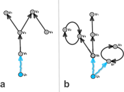
Figure 1: (a) A digraph with a single root. Network vertices and edges are shown in grey; driving vertices and edges - in blue. Vertex $\{V_{4}\}$ is inaccessible from the driving vertex $\{U_{1}\}$. Vertices $\{V_{1},V_{3},V_{2}\}$ form a dilation. (b) Elementary path $\{V_{6},V_{3},V_{1}\}$ and two elementary cycles $\{V_{2},V_{4}\}$ and $\{V_{5},V_{7}\}$ connected to the root $\{U_{1}\}$ form a cactus. This network is structurally controllable by a single drive.

Such a system may be represented with a directed graph (digraph) $G(\bf{A};\bf{B})=(V_{G};E)$, which structure doesn’t change in time. The vertex set $V_{G}=V\bigcup U$ includes both the state vertices $V$ corresponding to the $N$ vertices of the network, and the driving vertices $U$, corresponding to the $M$ input signals that are called the roots of the digraph $G(\bf{A};\bf{B})$. The edge set $E=E_{V}\bigcup E_{U}$ consists of the edges among state vertices $E_{V}$, corresponding to the connections of the network, and the edges connecting driving vertices to state vertices $E_{U}$. In this terms, Lin’s theorem is given as: The system $(\bf{A};\bf{B})$ is not structurally controllable if and only if it has inaccessible nodes or dilations Lin:74 .

A state vertex is inaccessible if there are no directed paths reaching it from the input vertices. An inaccessible vertex can not be influenced by driving signals, making the whole network uncontrollable. The digraph $G(\bf{A};\bf{B})$ contains a dilation if there is a subset of vertices $S\subset V$ such that the neighborhood set of $S$ has fewer vertices than $S$ itself. Roughly speaking, dilations are subgraphs in which a small subset of vertices attempts to rule a larger subset of vertices (see Fig. 1a).

This formulation is not practical, because doesn’t tell us how many driving signals we should have in a given network to make it controllable. Alternatively, we may state that: An LTI system $(\bf{A};\bf{B})$ is structurally controllable if and only if $G(\bf{A};\bf{B})$ is spanned by cacti.

A graph is spanned by a subgraph if the subgraph and the graph have the same vertex set. For a digraph, a sequence of oriented edges $\{v_{1}\rightarrow v_{2},...,v_{k-1}\rightarrow v_{k}\}$, where vertices $\{v_{1},v_{2},...,v_{k-1},v_{k}\}$ are distinct, is called an elementary path $C$. When $v_{k}$ coincides with $v_{1}$, the sequence of edges is called an elementary cycle $O$. For the digraph $G(\bf{A};\bf{B})$, let me define the following subgraphs: (i) a stem is an elementary path originating from an input vertex; (ii) a bud is an elementary cycle $C$ with an additional edge $e$ that ends, but does not begin, in a vertex of the cycle; (iii) a cactus is defined recursively: a stem $C$ is a cactus. Let $C$, $O$, and $e$ be, respectively, a cactus, an elementary cycle that is disjoint with C, and an arc that connects $C$ to $O$ in $G(\bf{A};\bf{B})$. Then, $C\cup\{e\}\cup O$ is also a cactus. $G(\bf{A};\bf{B})$ is spanned by cacti if there exists a set of disjoint cacti that covers all state vertices.

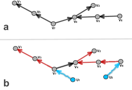
Figure 2: (a) A graph to find a minimum driver set. (b) Maximum matching is shown in red. Only two vertices $\{V_{6}\}$ and $\{V_{7}\}$ are unmatched. The network requires two independent drives/roots to be controllable.

A cactus is a minimal structure that contains neither inaccessible nodes nor dilations (see Fig. 1b). A complex network is unlikely to be spanned by a single cactus. But, it may be spanned by a few. Since the control of a single cactus requires a single root, to control a complex network we need as many driving signals as many cacti span the network. In practice, we want to find the minimal number of the driving signals to control a given network – the so-called minimum input problem Liu:16 . Hence, we need to find the minimal number of cacti to span a given network. At first glance, this combinatorial problem is a NP-hard, but in fact can be resolved in polynomial time with the maximum matching algorithm (see Fig. 2).

In a digraph, a matching is defined to be a set of directed edges that do not share common start or end vertices. A vertex is matched if it is the end vertex of a matching edge. Otherwise, it is unmatched. Maximum matching is a matching of the largest size. This definitions allow us to formulate the Minimum input theorem: To fully control a system $G(\bf{A};\bf{B})$, the minimum number of driver vertices is $N_{D}={\rm max}\{N-M,1\}$, where $M$ is the size of the maximum matching in $G(\bf{A};\bf{B})$. In other words, the driver vertices correspond to the unmatched vertices. If all vertices are matched $M=N$ (as in case of an elementary cycle), we need at least one input to control the network, hence $N_{D}=1$. We can choose any vertex as our driver vertex in this case. Note, that in general the maximum matching is not unique, i.e. the network may be controllable with different minimal sets of driver vertices. But, all these minimal sets are of the same size. The algorithm gives us the number and location of the drivers to apply to the network, hence concludes the study of the structural controllability.

In quantum networks, a vertex possesses a quantum system, such as atom, quantum dot or molecule. If two vertices are connected with an edge, they may communicate photons and classical information. An edge is directed according to the ability of a vertex to send photons to others. Classical information may be communicated between connected vertices both ways irrespective of edge directions. This setup fits most quantum communication protocols Nielsen:00 .

Because the quantum systems interact with each other and the environment, that may be present in the vertices, the quantum network dynamics is the subject of open quantum system dynamics Gardiner:00 , which is in general non-linear. However, there are few occasions, when the dynamics of an open quantum system may be described with linear differential equations as Eq. (1). For example, dissipative harmonic oscillator may be described with linear Master and Langevin equations Gardiner:00 . This type of quantum dynamics of the vertices we must imply to ensure that the quantum network can be described with Eq. (1). Whenever the behavior of a quantum system cannot be correctly described with a system of linear differential equations (1), further considerations are invalid.

The difference between classical and quantum networks is that the latter are non-local. This leads to the fact that distant vertices may become entangled and display correlated dynamics, even so they are not connected with an edge. The entanglement may appear spontaneously as a result of the non-linear dynamics Manz:13 or may be created by LOCC Acin:07 . The entanglement between distant vertices may be interpreted as a new edge of the network Acin:07 ; Siomau:16 . The direction of this entanglement edge is defined by the direction of the classical communication. The LOCC may be used to loop all inaccessible vertices and dilations into elementary cycles, modifying the network so, that it is spanned by a single cactus, i.e. all its vertices are matched.

To be specific, let us suppose that we have a connected quantum network represented by a digraph and of the same configuration as in Fig. 2a. We may investigate its classical structural controllability by executing the maximum matching algorithm to identify the minimal set of driving vertices. The network is spanned by two cacti, due to a dilation $\{V_{3},V_{7},V_{4}\}$. Let us choose one of the two elementary pathes, let say $\{V_{6},V_{5},V_{4},V_{2}\}$, and loop it into an elementary cycle by LOCC.

The procedure can be exemplified as follows. Suppose we have a quantum network consisting of three vertices $\{a,b,c\}$, so that $a$ is connected to $b$ and $b$ is connected to $c$. The quantum system at the vertex $a$ may be entangled with a quantum field mode, which is communicated to the vertex $b$. Subjected with the classical communication vertex $a$ is entangled with $b$, i.e. we created an entanglement edge. Through this edge, the quantum system at $b$ may influence the system at $a$ by performing local manipulation at $b$ and communicating information classically to $a$ Nielsen:00 . In this case, the direction of the classical communication sets the direction of the entanglement edge. If $a$ is entangled to $b$ and $b$ is entangled to $c$, we may apply entanglement swapping at $b$. This creates a non-local entanglement edge $a-c$. The edge may be directed both ways depending on the classical information flow.

Similarly, we may get rid of inaccessible vertices, in case of their presence. If we have a subgraph of inaccessible vertices in our connected graph, then there is at least one border vertex of the subgraph that has an edge directed from it to an accessible vertex. The inaccessible vertex may become entangled with the accessible vertex by LOCC. Hence, this two vertices are looped into an elementary cycle consisting of just two vertices. Iteratively, all the subgraph of inaccessible vertices may become accessible. As the result, the modified network is spanned by a single cactus, thus controllable by a single root. In general, the whole procedure can be executed for arbitrary two distant vertices in a finite connected network of size $N$ with at most $N^{3}$ LOCC Siomau:AIP .

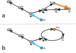
Figure 3: (a) By LOCC we may loop the elementary path $\{V_{6},V_{5},V_{4},V_{2}\}$ into an elementary circle increasing maximal matching of the quantum digraph. (b) The modification of the quantum digraph with LOCC may be viewed as creation of a supervertex $\{V_{2-6}\}$.

I showed that the restrictions of the Lin’s theorem, that are fundamental for classical networks, doesn’t apply to quantum networks. This is another radical difference between classical and quantum instances. The result is independent of the quantum network structure and is purely based on our ability to create nonlocal correlations with LOCC.

To make a conclusion about structural controllability of a network, we must be sure that the structure of the network doesn’t change in time. This may be guaranteed if the network is described with a system of linear equations. But, do LOCC change linearity of the quantum dynamical equations? Under some reasonable assumptions, the initial entanglement between two systems leaves the dynamical equations linear adding an inhomogeneous term Stelm:01 . But, this is an exception rather than the rule. Can we still conclude about the structural controllability? Yes, if we consider the entangled vertices as single super-vertex (see Fig. 3). Then, we must ensure that the super-vertex is coupled linearly to the neighbors, i.e. the output field operators of the super-vertex and the input field operators of the neighboring vertices are linearly dependant note . In this case the network remains linear, in spite of the non-liner internal dynamics of the super-vertex.

Structural controllability analysis is the very first step to evaluate network controllability. Although a network may be structurally controllable, for some combination of the dynamical parameters, it may not be controllable Liu:16 . Hence, we need to establish the so-called strong structural controllability, that is the network is controllable for any combination of the dynamical parameters. This analysis requires full information about the network parameters and analytical tools to process this information. The Kalman’s criterion of controllability Liu:16 is as fundamental as the Lin’s theorem for structural controllability, and may also fail as the latter, if applied to quantum networks. This urges a revision of our knowledge and strategies to establish control over complex quantum networks.

References

- (1) S.-K. Liao, et.al, Nature 549, 43-47 (2017).
- (2) H.J. Kimble, Nature 453, 1023 1030 (2008).
- (3) M.A. Nielsen and I.L. Chuang, Quantum Computation and Quantum Information (Cambridge University Press, Cambridge, 2000).
- (4) S. Perseguers, M. Lewenstein, A. Acin and J.I. Cirac, Nature Physics 6, 539-543 (2010).
- (5) G. Manzano et.al, Scientific Reports 3, 1439 (2013).
- (6) A. Acin, J.I. Cirac and M. Lewenstein, Nature Physics 3, 256-259 (2007).
- (7) M. Siomau, J. Phys. B.: At. Mol. Opt. Phys. 49, 175506 (2016).
- (8) C.-T. Lin, IEEE Trans. Auto. Contr. 19, 201-208 (1974).
- (9) Y.-Y. Liu and A.-L. Barabasi, Rev. Mod. Phys. 88, 035006 (2016).
- (10) C.W. Gardiner and P. Zoller, Quantum Noise: A Handbook of Markovian and Non-Markovian Quantum Stochastic Methods with Applications to Quantum Optics (Springer-Verlag, Heidelberg, 2000)
- (11) M. Siomau, AIP Conf. Proc. 1742, 030017 (2016).
- (12) P. Stelmachovic and V. Buzek, Phys. Rev A 64, 062106 (2001).
- (13) See section Cascaded Quantum Systems of Ref. Gardiner:00 for details.