The Inner 25 AU Debris Distribution in the $\epsilon$ Eri System

Abstract

Debris disk morphology is wavelength dependent due to the wide range of particle sizes and size-dependent dynamics influenced by various forces. Resolved images of nearby debris disks reveal complex disk structures that are difficult to distinguish from their spectral energy distributions. Therefore, multi-wavelength resolved images of nearby debris systems provide an essential foundation to understand the intricate interplay between collisional, gravitational, and radiative forces that govern debris disk structures. We present the SOFIA 35 ${\rm\mu m}$ resolved disk image of $\epsilon$ Eri, the closest debris disk around a star similar to the early Sun. Combining with the Spitzer resolved image at 24 ${\rm\mu m}$ and 15–38 ${\rm\mu m}$ excess spectrum, we examine two proposed origins of the inner debris in $\epsilon$ Eri: (1) in-situ planetesimal belt(s) and (2) dragged-in grains from the cold outer belt. We find that the presence of in-situ dust-producing planetesmial belt(s) is the most likely source of the excess emission in the inner 25 au region. Although a small amount of dragged-in grains from the cold belt could contribute to the excess emission in the inner region, the resolution of the SOFIA data is high enough to rule out the possibility that the entire inner warm excess results from dragged-in grains, but not enough to distinguish one broad inner disk from two narrow belts.

1. Introduction

Debris disks are integral parts of planetary systems. They are produced when larger objects, e.g. planets, stir planetesimal belts, causing a cascade of collisions that break minor bodies down into dust. More than 400 debris disks are known, providing a rich resource to study planetary system evolution and architecture (Matthews et al., 2014). However, the majority only have photometric points defining a general spectral energy distribution (SED). SEDs measure temperature, but grains with different optical properties can have the same temperature at different distances from a star, making SED modeling degenerate. Resolved images are essential to eliminate this degeneracy. The few systems that are close enough to be well resolved provide the foundation for the entire effort to interpret debris disk behavior in terms of the underlying planetary configuration. Because the huge range of particle sizes (from sub-$\mu$m to mm/cm sizes) produced in debris disks results in size-dependent dynamics influenced by various forces (radiation and drag), the observed disk structures are wavelength-dependent (e.g., Wyatt 2006). Therefore, multi-wavelength observations are essential to understand the intricate interplay governing debris disk structures.

The two benchmark nearby debris disks are not around sun-like stars, but are around the early A-stars Fomalhaut and Vega. These are aptly termed the debris disk twins, not only because of the similar stellar types, but their similar ages ($\sim$450 Myr), the evidence for warm belts, and their prominent cold belts (Su et al., 2013, 2016). They have a large gap between their warm and cold dust belts, a possible signpost for multiple, low-mass planets beyond the water-ice lines that typically lie near the warm belts (e.g., Quillen 2006; Su et al. 2013). The high temperatures ($\sim$9,000 K) and luminosities ($\sim$16 and $\sim$30 L_☉ respectively) of these stars subject their debris dust to different environments than for dust around the Sun – different not only in the radially-dependent equilibrium temperature, but also in the roles of photon pressure, magnetic fields, and stellar winds. Given that planetesimal belts probably form near the primordial ice line, the relatively weak dependence of this location on pre-main-sequence stellar luminosity (Kennedy & Kenyon, 2008) also potentially contributes to significant differences in the planetesimal belt environments.

Therefore, it is important to contrast debris systems around stars more like the Sun with those around Fomalhaut and Vega. Within 5 pc, $\tau$ Ceti (3.65 pc, van Leeuwen 2007) and $\epsilon$ Eri (3.22 pc, van Leeuwen 2007) are the only two low-mass stars with prominent debris disks. The age of $\tau$ Ceti (5.8 Gyr) results in a faint disk (Sierchio et al., 2014), greatly limiting the detectability of detailed disk structures. $\epsilon$ Eri provides a better translation from the debris properties of Vega and Fomalhaut to the environment of the solar system. It is at a similar age (400–800 Myr, Di Folco et al. 2004; Mamajek & Hillenbrand 2008) as Vega and Fomalhaut, but its temperature, mass, and luminosity (5,100 K, $M_{\ast}$=0.82 M_⊙, and $L_{\ast}$= 0.34 L_⊙) suggest that $\epsilon$ Eri should have similar properties with regard to magnetic field, stellar winds, and UV output as the early Sun.

Although the $\epsilon$ Eri debris disk has been resolved at multiple wavelengths, the structure of its debris system remains controversial. At 850 $\mu$m, JCMT/SCUBA revealed a nearly face-on, clumpy Kuiper-belt-like ring at a radius of $\sim$64 au (Greaves et al., 1998). The clumpy structure has been interpreted as evidence for an unseen planet interior of the cold ring (Ozernoy et al., 2000; Quillen & Thorndike, 2002; Deller & Maddison, 2005), but the perturbing planet remains undetected (e.g., Janson et al. 2015 and references therein). The large cold ring at 64 au is confirmed in the mm (Lestrade & Thilliez, 2015; MacGregor et al., 2015). From these images, it appears that many of the clumps can be ascribed to chance alignment with background galaxies (Chavez-Dagostino et al., 2016).

Spitzer imaging and spectroscopic data combined with a SED model suggest the existence of two distinct belts in its inner 25 au region (Backman et al., 2009). In the Backman model, the inner warm belt is similar in location to our own Asteroid belt located at $\sim$3 au, while the outer warm belt lies close to where Uranus orbits in our solar system ($\sim$20 au). The exact location and the width of the two inner warm belts as proposed by Backman et al. (2009) are only constrained by marginally resolved images and the SED modeling with assumed grain properties, and could be uncertain by factors of two. Recent Herschel far-infrared images of the system suggest the outer warm belt may be as close as 12–16 au (Greaves et al., 2014).

Hatzes et al. (2000) reported the detection of a planet, $\epsilon$ Eri b, whose orbit (Benedict et al., 2006) may cross the innermost warm belt proposed by Backman et al. (2009), leading to an unstable configuration (Brogi et al., 2009). To avoid this difficulty, Reidemeister et al. (2011) instead suggested that the warm excess originates from small ($\lesssim$10 $\mu$m) grains in the cold outer belt, which are transported inward by Poynting-Robertson (P-R) and stellar wind drag. According to this hypothesis, the disk surface density is expected to be relatively flat between the warm and cold components while the radially dependent dust temperatures result in a centrally peaked 24 $\mu$m image. Under this model, there is no need for an inner planetesimal belt as the source of the warm dust. However, Butler et al. (2006) suggest that the planet’s orbit is much less eccentric, even consistent with being circular, which might make this model unnecessary. There is also controversy over whether the planet is real (Zechmeister et al., 2013), suggesting an alternative solution to the dilemma.

To better understand the debris distribution in the inner 25 au region of $\epsilon$ Eri, we obtained SOFIA 35 $\mu$m images of this system with a resolution of 3$\farcs$4. The details of the observations and data reduction, including the archival observations of calibrators, are presented in Section 2. A detailed characterization of the SOFIA 35 $\mu$m Point Spread Function (PSF) allows us to assess the disk extent at this wavelength, and show that the emission is centrally peaked but extends beyond two resolution elements, and then drops off quickly outside 10″ (Section 3). We analyze the disk radial profiles in the mid-infrared (with additional archival Spitzer MIPS 24 $\mu$m and IRS data) in Section 4. In Section 5, we use the 24 and 35 $\mu$m disk radial profiles to test three different debris distributions proposed in the literature, and suggest that the inner warm dust originates from one or two planetesimal belts lying within 25 au of $\epsilon$ Eri. We discuss the degeneracy in our choices of model parameters in Section 6 and conclude the paper in Section 7.

2. FORCAST Observations and Data Reduction

$\epsilon$ Eri was observed with the NASA Stratospheric Observatory for Infrared Astronomy (SOFIA, Gehrz et al. 2009; Young et al. 2012) during cycle 2 and 3 using the FORCAST instrument (Herter et al., 2012) in the F348 filter ($\lambda_{eff}$= 34.8 ${\rm\mu m}$, $\Delta\lambda$= 3.8 ${\rm\mu m}$) of the Long Wave Camera (LWC), resulting in a 3$\farcm$4$\times$3$\farcm$2 instantaneous field of view with 0$\farcs$768 pixels after distortion correction. The chopping was done with the Nod-Match-Chop (NMC) configuration with a chop throw of 60″ and a chop angle of 30° in the array coordinates to cancel atmospheric emission. A five-point dither pattern with an offset of 10″ in both RA and Dec directions was used to correct for array artifacts. Details about the observations are given in Table 1. The data were calibrated and reduced with the pipeline software (ver. 1.1.0) by the SOFIA Science Center.

To assess the presence of any extended emission structure around $\epsilon$ Eri, we also performed similar data reduction on archival calibration data obtained with the F348 filter during cycle 2 and 3, which include a handful of stellar calibrators (blue PSF sources) and the asteroid Ceres (red source).

Table 1Observational Log

#	Flight	Date	UT Time	FWHMx	FWHMy	$\sigma_{sky}$	Integration†
				[arcsec]	[arcsec]	[mJy arcsec-2]	[sec]
1	190	2015-01-29	05:02:38.8	4.51	3.15	6.64	1162
2	190	2015-01-29	05:29:09.6	4.32	3.48	5.75	1290
3	190	2015-01-29	05:59:43.5	4.26	3.43	6.37	1162
4	190	2015-01-29	06:25:51.9	3.53	3.11	7.10	1032
5	190	2015-01-29	06:52:34.9	3.64	3.28	6.21	1162
6	190	2015-01-29	07:19:24.5	4.60	2.64	7.26	774
7	191	2015-02-04	04:08:12.2	4.42	3.77	6.58	1678
8	191	2015-02-04	04:36:37.4	3.57	3.26	7.11	1420
9	254	2015-11-04	06:44:39.5	3.79	3.57	2.69	4368
10	258	2015-11-13	06:32:55.6	4.70	3.91	3.12	4048

2.1. $\epsilon$ Eri

The pipeline-produced Level-3 data products (i.e., nod-subtracted, dithers aligned, flux calibrated merged data) were the basis for further analysis (coadding and custom background subtraction). The $\epsilon$ Eri observations consist of 10 Level-3 images. Visual inspection of these images found one of the Level-3 products (#6, with the shortest total on-source integration time) has elongated image shapes. We did not use these data for the final coadd. We coadded the good images at subpixel levels with two different registration methods. The first method was to define the centroid of the source by fitting a 2-D Gaussian profile to the 10$\times$10 pixel area centered on the source. The measured Full Width at Half Maximum (FWHM) of the source in each of the images is given in Table 1. The average FWHM is 4$\farcs$1$\times$3$\farcs$4 $\pm$ 0$\farcs$4$\times$0$\farcs$3; on average, there is 9% variation in source FWHM among the 9 good images. The second method was to determine the sub-pixel shifts by cross correlating the central 10$\times$10 pixel area centered around the source. In both methods, each of the images was registered in sub-pixel levels, and then coadded with weights determined by its integration time.

The flatness of the background in the vicinity of the target is an important factor to assess the extension of the $\epsilon$ Eri disk. We used a custom sky subtraction program to take out the large-scale background structure in the final coadded data by fitting a low-power, two-dimensional polynomial on the coadded image with the source region (central 38$\farcs$4 region) masked out. The final sky-subtracted coadded data are slightly different depending on the registration methods. We will discuss the subtle difference in Section 3.2.

2.2. PSF Calibrators - Ceres and Stellar Sources

The SOFIA PSF is not as stable as space-based observatories given that it is an airborne facility. Therefore, it is important to evaluate the instrument PSF using point-source observations like Ceres and stellar calibrators. Ceres was observed eight times with the F348 filter as a low-temperature flux calibrator during FORCAST flights in 2015. In addition, stellar calibration observations with the same filter in 2015 are also included in our analysis: six $\alpha$ Boo, two $\alpha$ Tau, two $\beta$ UMi, and one $\gamma$ Dra. We determined the PSF variation by comparing the FWHM of these data using the same method as in $\epsilon$ Eri. The average FWHM of the Ceres data is 3$\farcs$61$\times$3$\farcs$42 ($\pm$0$\farcs$28) with a variation of $\sim$8%. The average FWHM of the stellar calibrator data is 3$\farcs$37$\times$3$\farcs$15 ($\pm$0$\farcs$20) with a variation of 6%. This suggests that the typical PSF variation in the SOFIA data is 6–8% for the central core (bright) region. We then combined the stellar observations to build a high signal-to-noise (S/N) PSF to assess the variation in the wing (faint) part of the PSF. Since the stars have various brightnesses, and these data were obtained at various altitudes (not flux calibrated), each individual Level-3 mosaic was first normalized before combining. The normalization is based on the core flux within a small aperture (radius of 2.5 pixels = 1$\farcs$92). Since the S/N in each individual image is relatively high for these bright targets, the centroiding methods make no difference in the final coadded data. We generated two final coadded PSFs: one for Ceres and one for all stellar calibrators together. We also applied an additional sky subtraction as in the $\epsilon$ Eri data for both coadded PSF data sets. Since both PSFs and our $\epsilon$ Eri data are coadded from many individual observations, the variation in the PSF should average out. Based on the final combined PSF data, it appears that Ceres is slightly broader than the stellar calibrator (as judged by the measured FWHM). A detailed comparison between the stellar and Ceres PSFs is given in Section 3.1.

3. FORCAST Mid-Infrared Imaging Results

3.1. FORCAST 35 ${\rm\mu m}$ Point-Spread Function

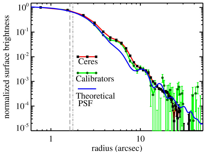
Figure 1.— Radial profiles of the point spread function (PSF) for FORCAST/SOFIA at 34.8 ${\rm\mu m}$ obtained with the Ceres and stellar calibrators. The theoretical PSF profile (blue solid line) computed by our custom IDL code is also shown for comparison. The vertical dashed and dotted-dash lines mark the FWHM of the stellar and Ceres PSFs, respectively. Our hybrid PSF is a combination of the stellar calibrators (for the region inside 10″) and the theoretical PSF (for the region outside 10″) (details see Sec 3.1).

To evaluate the FORCAST 35 ${\rm\mu m}$ PSF, we generated a theoretical PSF using a custom IDL code with inputs of a wavelength and jitter value to mimic the actual observations. We generated 50 PSFs at wavelengths across the F348 filter, and coadded them with weightings according to the filter transmission to get a composite PSF. We found that a jitter value of 1$\farcs$75 and a boxcar smooth factor of 3.4 pixels produce a good match in terms of measured FWHM with the observed stellar PSF.

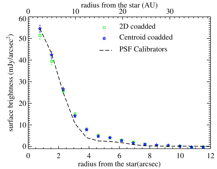
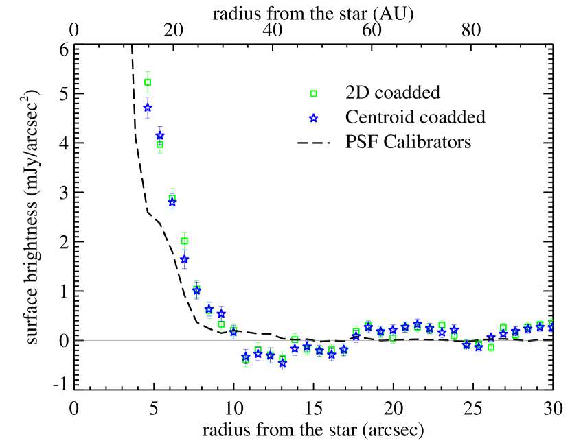
Figure 2.— The comparison of the radial profiles for $\epsilon$ Eri using two different registration methods. The hybrid PSF profile (normalized to the peak, which is 21% higher than the expected photosphere) is shown as the black dashed line. The left panel covers the central 12″ region, while the right panel shows the full radial range up to 30″ but with a smaller vertical range of flux. All error bars are shown as 1$\sigma$. There are some coherent up and down patterns outside 10″, which are consistent with the flat fielding residuals and within 3$\sigma$ of being zero.

We compared the two observed PSFs and the theoretical PSF in terms of azimuthally averaged radial profiles computed as follows. We first created a series of concentric rings with a width of 1 pixel (0$\farcs$768) about the source centroid (determined by the 2-D Gaussian fit), and computed the average value of all the pixels that fall in each ring. The measurement error at each radius is the standard deviation of all pixels in that ring, divided by the square root of the number of pixels in the ring. Since the FORCAST data are in the background limited regime, the background noise also contributes to the average flux measurement error. The background noise per pixel is found by computing the standard deviation of the pixels on a part of the blank region away from the source. The background noise per ring (i.e. background noise error) is estimated by taking the background noise per pixel and dividing it by the square root of the number of pixels in the ring. The total error in the average flux measurement per ring, therefore, is the measurement error and the background noise error added in quadrature. Figure 1 shows the normalized radial profiles for the PSF characterization. The high S/N of the Ceres data enable us to track the radial profile up to 25″ from the center, achieving a dynamical range of 10⁴. Overall, the observed PSFs (both Ceres and calibrators) match the theoretical one very well, except for the region at radii of 4″–10″. The exact reason of the mismatch is unknown, but probably related to how the data were taken and combined. As shown in Section 2.2, the Ceres PSF is slightly broader than the stellar PSF by 8% in the measured FWHM. Being a red source, Ceres is expected to be slightly larger due to diffraction across the bandwidth of the filter. However, the color difference can only account for a 2% difference between 5000 K and 200 K sources. Ceres had an apparent diameter of 0$\farcs$7 around the time of observations, which can account for an additional 2% difference in measured FWHM. The rest of this discrepancy is most likely due to telescope tracking errors unique to the Ceres observations. The SOFIA telescope uses a different technique to track on non-sidereal targets and the tracking can be slightly less accurate than sidereal tracking. Despite its high S/N, for this reason we cannot simply use Ceres as our PSF standard for model convolution (see Section 5). Instead, we constructed a hybrid PSF with the core (inner 10″) high S/N) region using the observed stellar PSF and the wing (outer 10″) region using the (noiseless) theoretical PSF. We used this hybrid PSF for all of the following analysis.

3.2. FORCAST 35 ${\rm\mu m}$ Image of $\epsilon$ Eri

The subtle difference between the two registration methods in combining the $\epsilon$ Eri data is best shown in the measured FWHM and the azimuthally averaged radial profiles for the image of the star (Figure 2). The left panel of Figure 2 shows the central 12″ region, and the right panel shows the full range up to 30″. The centroiding method gives a slightly sharper image by $\sim$3.5% (FWHM = 3$\farcs$63$\times$3$\farcs$48), but the surface brightness agrees within 1$\sigma$ as shown in the radial profiles. The profile outside 10″ is within 3$\sigma$ of zero and is consistent with no signal within the expected uncertainties in flat fielding. Therefore, we only concentrate our further analysis for the region inside a radius of 10″ around $\epsilon$ Eri.

Compared to the profile of the stellar calibrators (i.e., the hybrid PSF), the $\epsilon$ Eri profile is slightly extended in the range of 4″–10″ from the star. The slight extension is mostly evident at radii of 3″–5″ (10–16 au at the distance of $\epsilon$ Eri), and is independent of the registration methods. For simplicity, we adopt the centroiding coadded image for further analysis. The final coadded image of the $\epsilon$ Eri system is shown in Figure 3. The stellar photosphere of $\epsilon$ Eri is estimated to be 0.81 Jy at 34.8 $\mu$m (Section 4.1). The total flux within 10″ is 1.30 $\pm$ 0.09 Jy, suggesting that we detect an inner ($<$30 au) excess that is slightly more extended than the PSF.

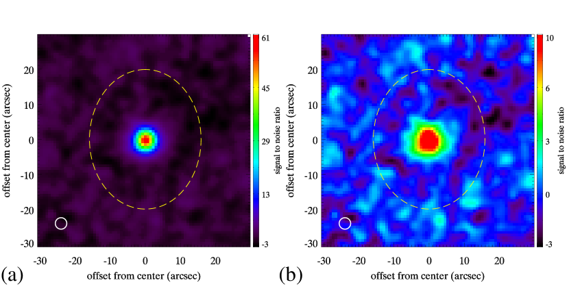
Figure 3.— SOFIA 34.8 ${\rm\mu m}$ image of the $\epsilon$ Eri system. Both images were smoothed by a Gaussian kernel of 1.5 pixels. The color scale is shown in units of signal-to-noise ratio with 1 $\sigma$ of 0.6 mJy/arcsec². The white circle in the left corner in both panels shows the beam size of the F348 filter, while the dashed yellow ellipse marks the inclined 64-au cold Kuiper-belt analog. The left panel (a) shows the final coadded mosaics before stellar subtraction while the right panel (b) shows after.

4. Analysis

To quantify the amount and structure of the excess emission, the stellar contribution needs to be subtracted from the image. To aid in characterizing the inner 25 au of the debris structure in the $\epsilon$ Eri system, we also include a re-analysis of the IRS spectrum and MIPS 24 ${\rm\mu m}$ image of the system (previously published in Backman et al. (2009)). In Section 4.1, we derive the photospheric flux at both bands. We then assess the excess emission by performing PSF subtraction at 35 ${\rm\mu m}$ in Section 4.2 and at 24 ${\rm\mu m}$ in Section 4.3. The re-analysis of the IRS spectrum is presented in Section 4.4 where we demonstrate the mid-infrared excess is consistent with dust emission with a temperature of 150$\pm$20 K.

4.1. Photospheric Fluxes

We estimated the photospheric output of $\epsilon$ Eri as follows. Since the star is only slightly cooler than the Sun, we used the carefully determined SED of the Sun as a starting point (Rieke et al., 2008). We took the effective temperature of the Sun to be 5780 K and adjusted the overall shape of the assumed SED of $\epsilon$ Eri by the ratio of blackbodies, one at the temperature of the Sun and the other at a temperature assigned for $\epsilon$ Eri. We left the latter temperature as a free parameter and varied it to minimize $\chi^{2}$ as determined relative to photometry of the star at $H$, $K_{S}$, Spitzer IRAC1, IRAC3, IRAC4, WISE W3, and W4. We omitted the IRAC2 band because it contains the CO fundamental absorption, which we expect to be deeper in $\epsilon$ Eri than in the Sun. We found a sharp minimum in $\chi^{\mathrm{2}}$ at a temperature of 5127 K, which is in satisfactory agreement with the nominal temperature for a K2V star (the type of $\epsilon$ Eri, Di Folco et al. 2004) of 5090K. The photospheric flux densities indicated by this procedure are 0.81 Jy at 34.8 $\mu$m (FORCAST F348 band), and 1.74 Jy at 23.68 $\mu$m (MIPS 24 $\mu$m band).

4.2. Excess Emission at 35 ${\rm\mu m}$ 

To characterize the excess emission at 34.8 $\mu$m near the star, PSF subtraction is necessary. We scaled the hybrid PSF to match the photosphere of $\epsilon$ Eri by normalizing its total flux within an aperture of 12″ to be 0.81 Jy without sky annulus (the sky is zero in the hybrid PSF). To account for the absolute flux calibration uncertainty, which includes (1) the photospheric prediction, 2%, and (2) the FORCAST flux calibration 6%, the PSF subtraction was also performed after scaling the hybrid PSF within $\pm$6.3% of the nominal photospheric value, allowing us to set the lower and upper boundaries of the uncertainty in the PSF-subtracted image. The nominal photospheric subtracted image is shown in Figure 3b, and the excess-only radial profiles are shown in Figure 4. The resultant peak flux in the excess-only profiles varies by 30–40%, depending sensitively on the exact scales of the PSF fluxes. However, these differences decrease significantly for the region outside the FWHM of the beam (i.e., outside a radius of 2″). We also evaluated the impact from the variation of the PSF FWHM (8%, see Section 2.2) in the photospheric subtraction. Using a narrower PSF, the resultant disk flux near the core is expected to be lower while the flux outside the core region would be slightly higher. Using a broader PSF, the resultant disk profile should have an opposite effect (i.e., higher flux near the core and slightly lower flux outside the core). We tested the changes by artificially broadening and sharpening the scaled PSF by 8%, and found that the resultant disk profiles are still within the uncertainty boundary set by the absolute flux calibration. Therefore, the extension (compared to the PSF profile) beyond 2″is robust, not subject to the uncertainties in absolute flux calibration nor to the PSF subtraction.

The excess emission is resolved at 34.8 $\mu$m by $\gtrsim$ 2 beam widths (i.e., the emission region is extended beyond 10 au). The excess flux at 34.8 $\mu$m within 10″ is 0.49$\pm$0.09 Jy, 60% of the stellar photospheric output. The observed profile is consistent with (1) a broad Gaussian structure peaked at the star, with a width of 18 au (green line in Figure 4), or (2) an unresolved source at the center plus a Gaussian-profile ring peaked at 10 au, with a width of 10 au. In summary, the SOFIA data confirm the excess emission near the star within 20 au, but cannot differentiate whether the emission region is one broad ring or composed of two separate structures (e.g., an unresolved source plus a ring).

Figure 4.— Excess-only profiles of the $\epsilon$ Eri system at 34.8 ${\rm\mu m}$ after photospheric subtraction (nominal and $\pm$6.3% the photospheric values. The PSF profile (normalized to the peak) is shown as the dashed line. The excess emission is resolved at 34.8 ${\rm\mu m}$, which could arise from (1) a central broad ring with a width of $\sim$18 au, shown as the green line, or (2) one point source plus a ring peaked at 10 au (not shown, see details in Section 4.2).

4.3. Excess Emission at 24 ${\rm\mu m}$ 

We searched the Spitzer archive and found unpublished MIPS 24 $\mu$m data (AOR 8969984), which account for an additional 50% of integration depth in addition to the published data (AOR 4888832) presented in Backman et al. (2009). We used the MIPS instrument team in-house pipeline (Gordon et al., 2005; Engelbracht et al., 2007) to reprocess these data to correct for instrument artifacts, and combined all data into a final mosaic. The combined data appear to be point-like, but with a FWHM of 5$\farcs$71$\times$5$\farcs$63, slightly extended compared with a typical point source (5$\farcs$50$\times$5$\farcs$42). We subtracted the photospheric contribution by scaling a blue calibration PSF to the estimated photospheric value (1.74 Jy). The photospheric subtracted image has a FWHM of 7$\farcs$17$\times$6$\farcs$89, much broader than that of a point source.

To characterize the excess emission at 24 $\mu$m further, we computed the azimuthally averaged radial profiles of the excess emission, shown in Figure 5. As at 35 $\mu$m, the uncertainty in the photospheric profiles was estimated by repeating the analysis with adjustments of $\pm$2.8% in the nominal photospheric value (2% from the absolute flux calibration and 2% from the photospheric extrapolation). The new 24 $\mu$m surface brightness profile is very similar to the one published by Backman et al. (2009) (Figure 5), but the improved reduction substantially reduces the errors at larger radii (enhanced by 1/$\sqrt{N}$ where N is the number of pixels in each of the annuli). Compared to the profile of a point source, the photospheric subtracted image has the first and second dark Airy rings (corresponding to 20 au and 65 au in $\epsilon$ Eri) partially filled, supporting the evidence that the excess emission is slightly resolved in the MIPS 24 $\mu$m band.

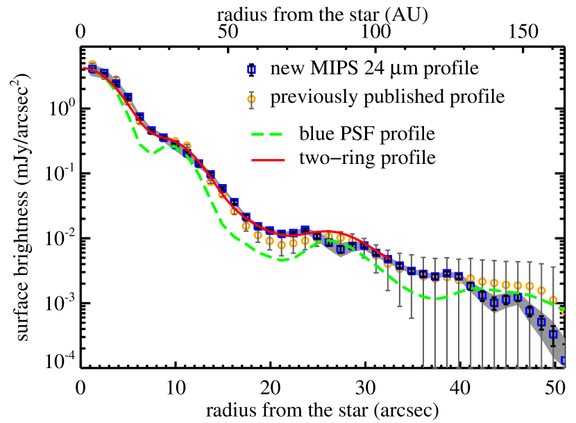
Figure 5.— Excess-only profiles of the $\epsilon$ Eri system at 24 ${\rm\mu m}$ after photospheric subtraction. The profile using the nominal photospheric value is shown as color symbols with circles for the new one produced in this work in comparison with the published profile (squares). The gray area around the new profile marks the uncertainty boundary due to photospheric subtraction and absolution flux calibration ($\pm$2.8% the photospheric values). The PSF profile (normalized to the peak) is shown as the solid green line. The first and second dark Airy rings are partially filled, suggesting the excess emission is slightly resolved at 24 ${\rm\mu m}$. The red line shows the resultant radial profile for a two-ring model (for details see Section 4.3).

To gain insights into the spatial distribution of the excess emission, we constructed a simple geometric two-ring model. The first ring is fixed at the star position with a specified width and represents the emission inside 20 au, and the second ring represents the emission from the cold Kuiper-belt-like ring, with a specified peak position and width. A final, high-resolution synthesized image is the sum of these two rings with a given relative flux ratio and a fixed total flux; i.e., there are four free parameters in this two-ring model: the width of the central ring, the peak position of the outer ring, the width of the outer ring, and the relative flux ratio. These high-resolution model images were then inclined to view at 30° from face-on, and convolved with the 24 $\mu$m PSF to simulate the observations.

We varied the four model parameters to minimize $\chi^{2}$ relative to the observed radial profile within 25″. We found that a central ring with a radius of $\sim$13 au and an outer ring peaked at 64 au with a width of $\sim$24 au can fit the observed radial profile relatively well (red line in Figure 5). It is reassuring that the peak position of the outer ring is found to be similar to the location found in other studies ($\sim$64 au, Backman et al. (2009); MacGregor et al. (2015); Chavez-Dagostino et al. (2016) ). However, as in the 35 $\mu$m profile analysis, this does not indicate there is only one inner excess region, but only that the inner excess emission region is extended at least to $\sim$13 au.

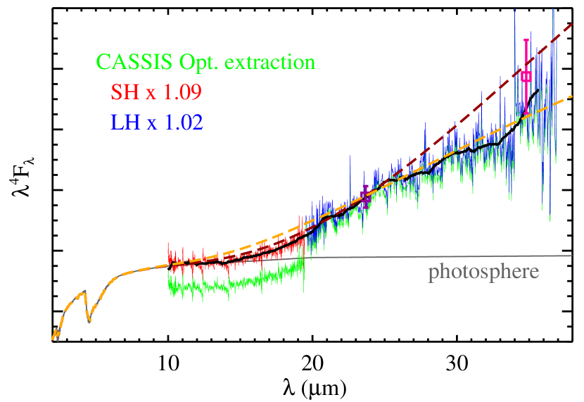
Figure 6.— Spitzer IRS high-resolution spectrum of $\epsilon$ Eri in $\lambda^{4}F_{\lambda}$ vs. $\lambda$ format so a Rayleigh-Jeans spectrum is flat. The MIPS 24 and FORCAST 35 ${\rm\mu m}$ photometry is shown as squares for reference. The green color shows the CASSIS optimal extraction spectrum. The red and blue color lines are the scaled SH and LH modules, respectively (see Section 4.4 for details). The final combined (joined and smoothed) spectrum is shown as the thick black line. The two dashed lines are the sum of the photosphere and a blackbody emission of 130 K (orange color) and 170 K (brown color). The excess emission is consistent with a blackbody emission of $\sim$150$\pm$20 K.

4.4. Spitzer IRS High-Resolution Spectrum

Details about the Spitzer IRS observations were given in Backman et al. (2009). As stated in that paper, linearity and saturation are an issue in the IRS low-resolution data. Therefore, we only discuss the high-resolution data (SH: 9.9–19.5 ${\rm\mu m}$ with a slit size of 4$\farcs$7$\times$11$\farcs$3 and LH: 18.7–37.2 ${\rm\mu m}$ with a slit of 11$\farcs$1$\times$22$\farcs$3). We retrieved the extracted high resolution spectrum from the CASSIS website and used the “optimal” product which simultaneously determines the source position and extraction in the two different nod observations. As described in Lebouteiller et al. (2015), this mode of extraction produces the best results when the source is resolved but only marginally extended. The CASSIS spectrum is shown in Figure 6 in the $\lambda^{4}F_{\lambda}$ vs. $\lambda$ format so a Rayleigh-Jeans spectrum is flat. There is a flux jump between the two SH and LH modules: the SH part of the spectrum is lower than the expected photosphere determined in Section 4.1, and the LH part of the spectrum is slightly lower than the MIPS 24 ${\rm\mu m}$ photometry. We joined the two modules by (1) scaling the SH module by 1.09 so that the 10–12 ${\rm\mu m}$ region matches the expected photosphere level, and (2) scaling the LH module by 1.02 so it matches the MIPS 24 ${\rm\mu m}$ photometry. The scalings are within the uncertainty in the absolute flux calibration between the MIPS and IRS instruments.

We used the final combined and smoothed (to R = $\lambda/\Delta\lambda\sim$30) spectrum (the black line in Figure 6) to estimate the dust temperature of the excess emission. Although the excess is not exactly blackbody-like, the excess emission can be described by a blackbody emission with temperatures between 170 K and 130 K. In Figure 6, we overplotted two (dashed) curves to represent the sum of the photosphere and a blackbody emission of 170 K and 130 K (both normalized to the MIPS 24 ${\rm\mu m}$ photometry point). This comparison suggests that the excess emission is consistent with a dust temperature of $\sim$150$\pm$20 K.

For blackbody-like emitters (1 mm astronomical silicates), these temperatures correspond a stellocentric distance of 1.5–2.5 au; however, for 1 ${\rm\mu m}$ silicate-like grains the corresponding distance is larger ($\sim$2–3.5 au) (see Figure 7). This temperature-radius relation is also composition dependent. In Figure 7 we show the temperature distributions using icy silicates (90% of ice by volume). Icy grains are generally poor absorbers; therefore, at the same temperature they are located at smaller stellocentric distances compared to the same size, bare silicates.

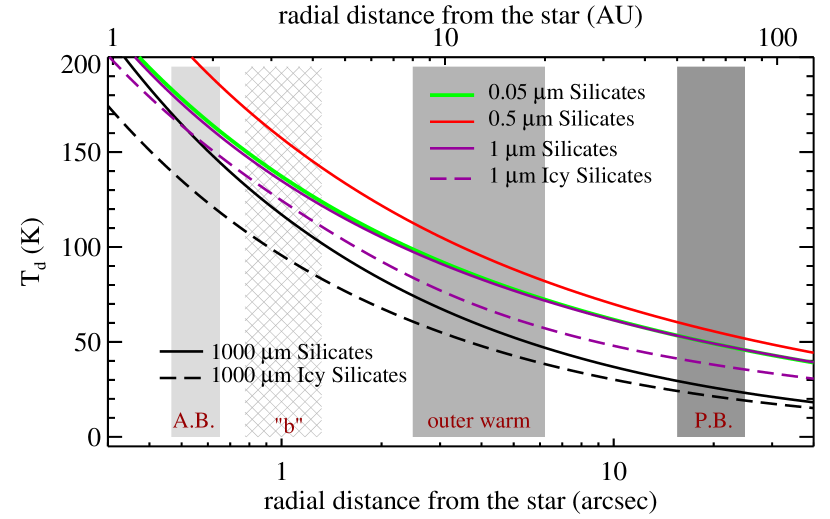
Figure 7.— Dust temperature distribution for both astronomical silicates and icy silicates for selected grain sizes around $\epsilon$ Eri. The chaotic zone of the putative $\epsilon$ Eri b is marked as the hashed area. The two light gray areas represent the two distinct dust belts (asteroid belt (A.B.) and outer warm belt) that are consistent with the presence of $\epsilon$ Eri b (see Section 5.3 for details). The dark gray area marks the Kuiper-belt-like planetesimal belt (P.B.).

5. Model Comparison

Based on the analysis presented in Section 4, it is evident that there is a substantial amount of excess emission in the inner 25 au of the $\epsilon$ Eri system, which is resolved by FORCAST at 35 $\mu$m and MIPS at 24 ${\rm\mu m}$ (at a linear resolution of $\sim$ 11 au). We refer to this excess emission as the “warm” excess to differentiate it from the cold excess emission from the 64 au Kuiper-belt-like ring. Two different scenarios have been suggested for the origin of the warm excess around $\epsilon$ Eri: (1) in-situ planetesimal belt(s) and (2) grains dragged in from the cold Kuiper-belt-like belt. Using the newly obtained mid-infrared disk radial profiles, we test these proposed models in the following subsections to probe the nature of the warm excess around this star.

We test the models proposed by Backman et al. (2009), Reidemeister et al. (2011) and Greaves et al. (2014) for the inner 25 au region. High-resolution face-on model images at 23.68 $\mu$m and 34.8 $\mu$m are constructed based on the parameters given in those papers. Each of the models also reproduces the system’s SED globally when additional components are added. We explore two different grain properties: astronomical silicates (Laor & Draine, 1993) and a mixture of silicates and organics (Ballering et al., 2016) to fit the mid-infrared disk profiles. We find that the choice of the grain types and properties has only a small impact on the resultant model images at these wavelengths. Given the degeneracy, we only show the model results using astronomical silicates. Furthermore, icy silicates are used when computing the SEDs for the components beyond the ice line (radial location $>$ 4 AU, e.g., the cold planetesimal belt and outer warm belt). The high resolution, face-on model images are then inclined to view at 30° from face-on and convolved with instrumental PSFs to simulate the observations. We compare the model radial profiles with the observed ones for each case. Since we only focus on the nature of the warm excess, the comparison was only done for the disk surface brightness profile within $\sim$10″ (30 au).

5.1. Dragged-in Grains as Proposed by Reidemeister et al. (2011)

The stellar wind drag for $\epsilon$ Eri is found to be 28 times stronger than the P-R drag, based on the measured mass-loss rate 30 times higher than that of the Sun (Wood et al., 2002) and the average solar wind velocity. Therefore, a significant inward flow of dust grains from the cold Kuiper-belt-like region is expected, unless there is a massive, shepherding planet interior of the cold belt. Assuming no such planet, Reidemeister et al. (2011) modeled the marginally resolved Spitzer 24, 70 and 160 $\mu$m images and found that the Spitzer data are consistent with this possibility.

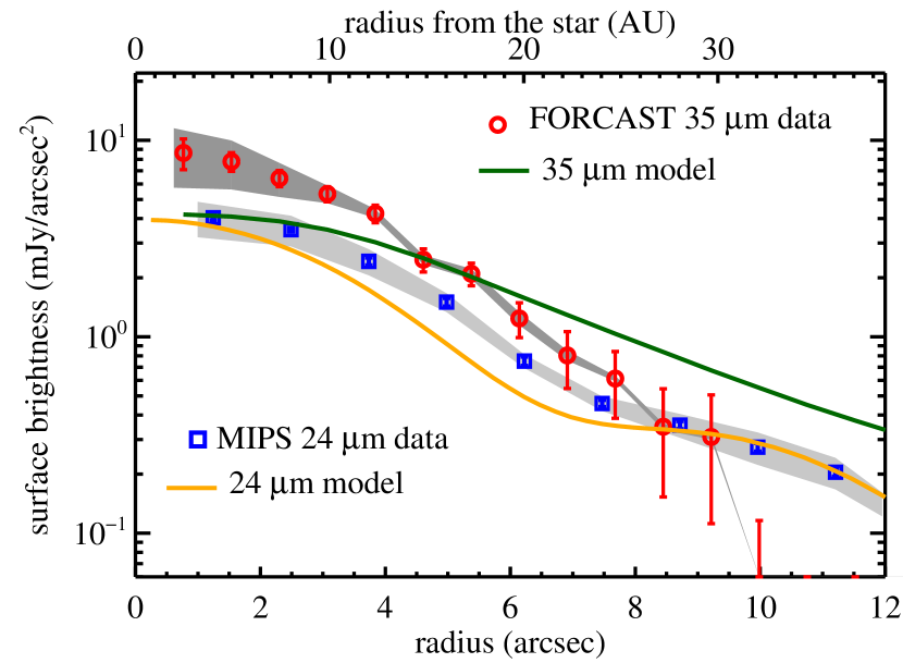
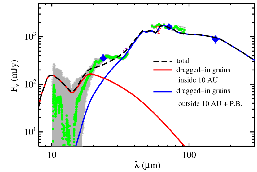
Figure 8.— Model results using the parameters from Reidemeister et al. (2011) in comparison with the observed disk profiles (upper panel) and the SED (bottom panel). In the disk profile plot, the observed profiles are symbols with gray areas marking the upper and lower boundaries of uncertainty due to flux calibration and PSF subtraction. Red circles are the FORCAST 35 ${\rm\mu m}$ data, and blue squares are the MIPS 24 ${\rm\mu m}$ data. Model profiles are shown in solid lines with green color for 35 ${\rm\mu m}$ and orange for 24 ${\rm\mu m}$. In the bottom SED plot, the various symbols are the excess photometry measurements for the whole system, and the green dots with error bars are the excess from the IRS and MIPS-SED spectra. The gray area around the IRS excess spectrum represents the uncertainty associated with the stellar photospheric extrapolation and subtraction. The model SED is composed of two parts: the red (the dragged-in small grains inside 10 au) and blue solid lines (the rest of the dragged-in grains and the dust in the cold planetesimal belt (P.B.)) with the sum shown as the black dash line (replicated from the bottom panel of Figure 8 in Reidemeister et al. 2011).

Using the no-planet configuration (i.e., no dynamical perturbation in the dragged-in dust flow), we computed model images with parameters derived from Reidemeister et al. (2011) to compare with our new data. The derived radial disk profiles are shown in the upper panel of Figure 8 with the SED shown in the bottom panel. The model SED is a replicate of the bottom panel of Figure 8 in Reidemeister et al. (2011) using the same grain parameters and composition. The model disk surface brightness profile at 24 $\mu$m is consistent with the one published in Reidemeister et al. (2011) (i.e., the fit is good for the old, large error-bar profile). However, the 35 $\mu$m model disk profile under-predicts the disk flux within 4″ (12 au), and over-predicts it outside 6″ (20 au). The proposal by Reidemeister et al. (2011) that the entire inner warm disk could result from dragged-in grains is not consistent with the SOFIA measurements.

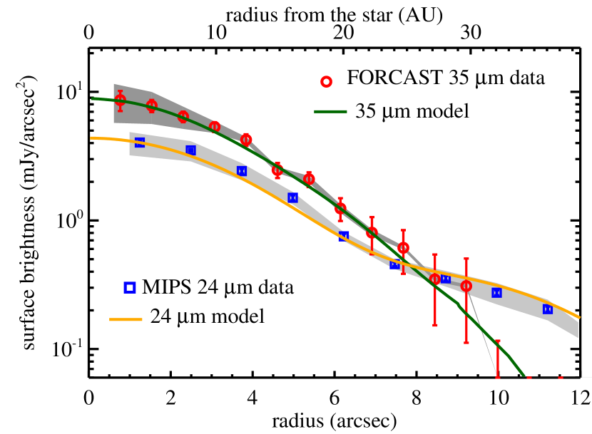
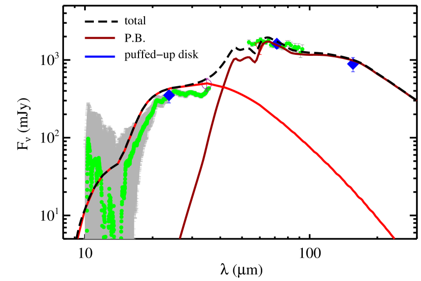
Figure 9.— Model results using the geometric parameters of Greaves et al. (2014) in comparison with the observed disk profile (upper panel) and SED (lower panel). Symbols and lines are the same as in Figure 8. In the bottom SED plot, the model SED for the puffed-up dust disk is shown as the red solid line and the broad cold disk is shown as the brown solid line with the sum shown as the black dashed line.

5.2. One Broad and Puffed-up In-situ Dust Belt as Proposed by Greaves et al. (2014)

Resolved images of $\epsilon$ Eri obtained by Herschel suggest inner excess emission at 70 and 160 $\mu$m. Greaves et al. (2014) modeled this inner excess as one single disk with simple geometric parameters: a wedged disk with a radial span of 3–21 au in an $r^{-1}$ density distribution and an opening angle of $\pm$23°. Note that the opening angle is quite large, i.e., the disk is vertically extended. Due to the significant scale height in this model, we computed the model images with the code dustmap ver. 3.1.2 (Stark, 2011), which can take a 3-D structure as an input, with the geometric parameters listed above and an inclination angle of 30°. We assumed grain parameters using compact astronomical silicates with a minimum grain size ($a_{min}$) of 1 $\mu$m, a maximum grain size ($a_{max}$) of 1000 $\mu$m, and a particle size power-law index ($q$) of –3.5. Figure 9 shows the results. This model fits the disk profiles very well (the upper panel of Figure 9), and reproduces the mid-infrared SED reasonably well with the normalization set by fitting the disk profiles. For the sake of completeness, we also computed the cold belt SED using the parameters given by Greaves et al. (2014) – a broad, geometrically thin disk from 36 to 72 au with a constant surface density. For this cold component, we used icy silicates with $a_{min}$ of 1 ${\rm\mu m}$ and $a_{max}$ of 1000 ${\rm\mu m}$ in a $q=-3.5$ size distribution. We did not include this component when computing the 24 and 35 ${\rm\mu m}$ disk profiles since its contribution is insignificant at these wavelengths. The combined SED fits the observed points satisfactorily. However, we note that the inner radius of this cold disk (36 au) is significantly smaller than the one inferred from the mm observations ($\sim$53 au from MacGregor et al. (2015), and $\sim$59 au from Chavez-Dagostino et al. (2016)). This might suggest that the broad, cold disk geometry is too simplistic, and a more complex distribution (e.g., a narrow cold belt plus an outer warm belt (see Section 5.3) or a small amount of dragged-in grain component) is needed.

The choice of $a_{max}$ has no impact on disk profiles nor the SED at the model wavelengths; however, the value of $a_{min}$ does make a noticeable difference at 24 $\mu$m and in the overall shape of the SED shortward of $\sim$20 $\mu$m. In general, the $a_{min}$ is usually set to the radiation blowout size ($a_{bl}=1.14\ Q_{pr}\ L_{\ast}\ M_{\ast}^{-1}\ \rho_{g}^{-1}$ where $\rho_{g}$ is the grain density and $Q_{pr}$ is the radiation pressure efficiency averaged over the stellar spectrum, and is assumed to be 1 for grain sizes comparable or larger than the wavelength where the stellar spectrum peaks (Burns et al., 1979)). However, as noted by Reidemeister et al. (2011) (Figure 2 in that paper), for the luminosity and mass of $\epsilon$ Eri, the blowout size does not exist. In the Reidemeister et al. (2011) model, $a_{min}$ was formally set to be 0.05 ${\rm\mu m}$, but much of the dust cross section in their modeled size distribution comes from larger, $\mu$m-sized grains (see their Figure 4). Setting $a_{min}$ to be 0.05 ${\rm\mu m}$ initially, we found that it is difficult to obtain simultaneous good fits to the disk profiles at both wavelengths; i.e., a good fit at 35 ${\rm\mu m}$ produces a too bright and broad MIPS 24 ${\rm\mu m}$ profile. Setting $a_{min}$ to larger sizes significantly improves the fit at 24 ${\rm\mu m}$ as shown in Figure 9. Setting different $a_{min}$ for the cold broad disk has no noticeable difference in the resultant SED. We will discuss the physical reason why a large $a_{min}$ is preferred around $\epsilon$ Eri in Section 6.1.

5.3. Two Narrow, In-situ Planetesimal Belts

The third model we tested is similar to the two-belt model proposed by Backman et al. (2009) based on the marginally resolved Spitzer images. As noted by Backman et al. (2009), the exact locations of the warm belts ($\sim$3 au and $\sim$20 au) are not well constrained by either the images or the SED. As suggested by the Herschel measurements, the outer warm component is likely to be smaller than was inferred from the Spitzer data. Greaves et al. (2014) suggest the warm planetesimal belt is located at 14 au with a width of 4 au. If the inner warm belt were a direct analog of our own Asteroid belt (near the ice line), the expected location should be 1.5–2 au simply from scaling by stellar luminosity. In fact, such a small size for the inner warm belt would be more consistent with the presence of $\epsilon$ Eri b (see discussion in Section 6.2).

In light of these results, we construct a revised two-belt model with the following parameters. Both belts are assumed to be geometrically thin (no scale height) and with a constant surface density, and to contain grains from $a_{min}=$ 1 $\mu$m to $a_{max}=$ 1000 $\mu$m in a power-law size distribution with $q$ set to –3.65 (e.g., Gáspár et al. 2012). The inner warm belt is assumed to range from 1.5–2 au, and the outer warm belt ranges from 8–20 au. Note that the outer warm belt appears to be broad, but most of the emission at the model wavelengths comes from the inner 8–12 au region due to radial dependence of the dust temperatures since we used a constant surface density. Furthermore, in order to produce overall good fit to the system’s SED, we have to use icy silicates for the outer warm belt to suppress the total flux in the mid-infrared while providing enough flux in the range of MIPS-SED spectrum (also see Figure 6 in Reidemeister et al. (2011)). Similarly, we also include a SED fit for the cold planetesimal disk ranging from 55 to 80 au (the radial span derived by MacGregor et al. (2015)) using icy silicates with the same grain size distribution as in the warm belts.

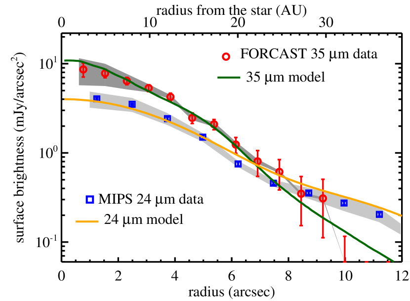
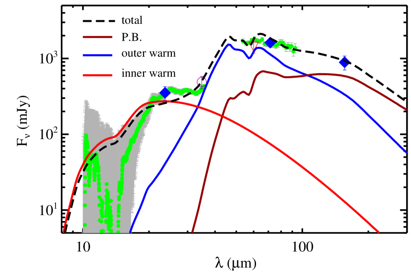
Figure 10.— Model results using the revised two-belt model with the locations slightly different from the ones of Backman et al. (2009). Symbols and lines are the same as in Figure 8. In the bottom SED plot, the two warm belts are shown as the red and blue solid lines, and the contribution from the dust in the 64 au belt is shown as the brown solid line. Similarly, the sum of these three components is shown as the black dashed line.

The resultant model profiles are shown in the upper panel of Figure 10 with the combined SED in the bottom panel. This revised two-belt model fits the 35 $\mu$m profile reasonably well (within 1$\sigma$), but is slightly too broad/bright outside 5″ at 24 $\mu$m (but still within 3$\sigma$). The largest issue with models of this class is that they fall slightly short of the measured SED between 20 and 30 $\mu$m, which might indicate that the assumed geometry is too simple, or might be revealing a problem for this type of model. We also produced the model fits for a larger (3–4 au) asteroid belt as originally suggested by Backman et al. (2009) with the same outer warm belt (3–20 au) and SED parameters. The results are very similar in the disk profiles with a slightly better SED fit in the 20–30 ${\rm\mu m}$ region. Limited by the uncertainty in the exact shape of the mid-infrared excess, both asteroid-belt models produce similar results.

5.4. Summary

We tested three proposed debris distributions in the inner 25 au of the $\epsilon$ Eri system using the newly obtained mid-infrared disk profiles. We found that the 24 and 35 $\mu$m emission is consistent with the in-situ dust distribution produced either by one planetesimal belt at 3–21 au (e.g., Greaves et al. 2014) or by two planetesimal belts at 1.5–2 au (or 3–4 au) and 8–20 au (e.g., a slightly modified form of the proposal in Backman et al. 2009). The observed profiles are not consistent with the case dominated by dragged-in grains (uninterrupted dust flow from the cold Kuiper-belt-analog region) as proposed by Reidemeister et al. (2011). This might suggest the need of a planet interior to the 64-au cold belt to maintain the inner dust-free zone, or a very dense cold belt where the intense collisions destroy the dust grains before they have enough time to be dragged in. In either case, some amount of dragged-in grains from the cold belt can still contribute a fraction of the emission inside 25 au; the exact amount remains to be determined by future high spatial resolution data and improved collisional models for the cold belt.

The model derived dust fractional luminosity ($f_{d}$) is 3$\times 10^{-5}$ and 7$\times 10^{-5}$ for the inner and outer warm belts, respectively, in the revised two-belt model. For the broad disk model, the dust fractional luminosity is 6$\times 10^{-5}$. We adopt the simple analytical model proposed by Wyatt et al. (2007) to test whether the dust in the inner $\epsilon$ Eri system is produced by transient events. Assuming the typical parameters for disks around solar-like stars and an age of 800 Myr, the maximum dust fractional luminosity ($f_{max}$) is 1$\times 10^{-6}$ and 4$\times 10^{-5}$ for a belt at 2 and 10 au. Therefore, the observed dust levels in these belts are close to the expected maximum value for dust being generated through collisional griding, and do not require to invoking transient events.

We note that the model parameters (especially the grain parameters) are not unique in our test cases due to degeneracy between grain properties and dust location. This is particularly true for the cold belt component since we do not include the image fits to the far-infrared and mm wavelength data (beyond the scope of the paper). For simplicity, we adopted the astronomical silicates as the grain composition in modeling the component inside 10 au. The mismatch in the 20–30 ${\rm\mu m}$ SED region might partially be due to this choice, in addition to the simple geometry assumed for the inner component. Furthermore, a larger (3–4 au) inner warm belt in the two-belt model produces similar results. Nevertheless, the existence of an inner (within 25 au) separate dust source (i.e., planetesimal belt(s) different from the outer cold belt) is a robust conclusion inferred from the newly obtained SOFIA data.

6. Discussion

6.1. Minimum Grain Sizes in the Inner Region of the $\epsilon$ Eri System

In Section 5, we showed that $a_{min}\sim$1 ${\rm\mu m}$ gives a much better fit to the mid-infrared disk profiles compared to the models using a smaller size cutoff in the particle size distribution. Observationally a wide range of $a_{min}$ has been inferred from resolved imaging and mid-infrared spectroscopy. Since silicate-like small grains have solid-state features in the 8–25 ${\rm\mu m}$ region, a featureless emission spectrum is usually interpreted to indicate a lack of small grains. However, the definition of “small” depends on the dust composition. For example, for amorphous silicates (like astronomical silicates), the 10 ${\rm\mu m}$ and 20 ${\rm\mu m}$ features have very similar shapes for grain sizes of 0.05–1 ${\rm\mu m}$ (with a slightly sharper 10 ${\rm\mu m}$ feature toward smaller sizes). As a result, at the same dust temperature the resultant emission spectrum is very similar, and the only difference lies in the amount of emission. Therefore, the IRS spectrum in the $\epsilon$ Eri inner region provides no constraint on the minimum grain size, as also has been suggested by Backman et al. (2009) (who found that the spectrum only requires $a\lesssim$3 ${\rm\mu m}$).

As discussed in Reidemeister et al. (2011), the nominal blow out size does not exist in $\epsilon$ Eri due to its low mass and luminosity. However, a possible blow out size might exist if pressure exerted by stellar winds is invoked. In a case where the contribution of the stellar wind is strong enough, a sum of the radiation pressure force and stellar wind pressure force could reinforce $a_{bl}$, as has been suggested in the AU Mic disk (Figure 1 in Schüppler et al. (2015)). However, for a K-star like $\epsilon$ Eri, the effect is too small, resulting again in no blow out limit.

Theoretically, we expect some depletion in the inner region around $\epsilon$ Eri due to enhanced drag forces (P-R and stellar wind drags). The P-R time scale depends on the mass of the star, the location of the dust ($R$) and the ratio between radiation force and gravity ($\beta\propto a^{-1}$), is given as

$$\tau_{PR}=400\ yr\ \frac{M_{\sun}}{M_{\ast}}(\frac{R}{AU})^{2}\frac{1}{\beta}\ .$$ (1)

Therefore, $\tau_{PR}\sim$4 $\times 10^{3}$ yr for a belt at 2 au around $\epsilon$ Eri (assuming $\beta$ = 0.5). Such a dust belt with a $f_{d}$ of 3$\times 10^{-5}$ has a collisional time scale of $\sim$4$\times 10^{4}$ yr, roughly 10 times longer than the P-R time scale. With the additional aid of stellar wind drag from the active star, the drag timescales will be even shorter. Since smaller particles are dragged in faster than larger ones, we expect a flatter size distribution at small sizes, setting an effective $a_{min}$ larger than the typical size in a collision-dominated system.

One can estimate $a_{min}$, or the dominant/critical grain size ($a_{c}$), by balancing the two source and sink time scales as suggested by Kuchner & Stark (2010) and Wyatt et al. (2011). In the inner region of $\epsilon$ Eri, the source time scale is the collisional time scale, and the sink time scale is the transported time scale by stellar wind since the stellar wind drag dominates the P-R drag. We then re-derived Eqn.(6) of Kuchner & Stark (2010) as follows:

$$a_{c}=1000\ \mu\rm{m}\ Q_{sw}\left({{\rho_{g}}\over{1\ \rm{g}\ \rm{cm}^{-3}}}\right)^{-1}\left(\dot{M}_{sw}\over 30\dot{M}_{\odot}\right)$$

$$\left({M_{\ast}\over{M_{\odot}}}\right)^{-1/2}\left({R\over{1\ au}}\right)^{-1/2}\left({f_{d}\over{10^{-7}}}\right)^{-1},$$ (2)

where $Q_{sw}$ is the stellar wind pressure efficiency, and $\dot{M}_{sw}$ is the stellar wind mass loss rate. Assuming $Q_{sw}$=1, $\rho_{g}$ = 2.5 g cm^-3, a mass loss rate of 30 times the solar value, M_∗ = 0.82 M_☉, $R$ = 2 au, and $f_{d}$ of 3$\times 10^{-5}$, the critical grain size is about 1 ${\rm\mu m}$.

Using the energy-conservation criterion, Krijt & Kama (2014) analytically derived the lower boundary of the particle sizes produced in debris disks. Under plausible parameters, they found that $a_{min}$ could be much larger than $a_{bl}$ depending on the collision velocity, material parameters, and the size of the largest fragment. Thebault (2016) numerically investigated such an effect, and concluded that the surface energy constraint generally has a weak effect for early-type stars and wide (50–100 au) debris disks, but might be more pronounced for sun-like stars and narrow belts. The depletion of the small grains is hard to estimate since we lack detailed information on the planetesimal belt(s) in the inner region of $\epsilon$ Eri. As an optimal case (since some parameters of their model are quite uncertain), the ratio between $a_{min}$ and $a_{bl}$ is $\sim$3 for a 2 au belt around $\epsilon$ Eri (0.34 L_☉ and 0.82 M_☉) (Eqn. (7) in Krijt & Kama 2014). Our choice of $a_{min}\sim$1 ${\rm\mu m}$ is consistent with this limit and the critical size estimated in the previous paragraph.

6.2. Putative $\epsilon$ Eri b and the Location of an Asteroid-belt Analog

The existence of $\epsilon$ Eri b and its orbital parameters have been heavily debated since it was reported in 2000 (Hatzes et al., 2000; Benedict et al., 2006; Butler et al., 2006). The Exoplanet Encyclopedia lists the planet at 3.5 au radius as confirmed, but Zechmeister et al. (2013) combined 15 years of radial velocity data and found that it did not support this status for the case of a highly eccentric orbit ($e\sim$0.6). A similar result was also been found by Anglada-Escudé & Butler (2012). Howard & Fulton (2016) analyzed all available radial velocity measurements from Lick and Keck Observatories by the California Planet Survey, and found that the stellar CaII H& K emission does not correlate with the radial velocity. Thus the radial velocity modulation is likely caused by an external source, i.e., the planet. Combining available ground-based high-contrast imaging, Mizuki et al. (2016) presented an updated contrast curve around $\epsilon$ Eri, and could marginally rule out the 1.6 M_J, $e=$0.7 case (Benedict et al., 2006) if the age of the system is as young as 200 Myr.

As noted by Backman et al. (2009), the possibility that $\epsilon$ Eri b is on a highly eccentric orbit is inconsistent with the existence of an inner warm debris belt at $\sim$3 au. If the planet co-exists with an asteroid-belt analog (i.e., one within 2 au), its orbit must have low eccentricity ($e\leq$0.2), based on the dynamical stability study by Brogi et al. (2009). We estimated the width of the planet’s chaotic zone by assuming $\epsilon$ Eri b is 1.6–1.7 M_J with $e$= 0–0.2. The inner boundary of the chaotic zone is then at 2–2.6 au, with 3.5–5 au for the outer boundary using the formulae from Mustill & Wyatt (2012) and Morrison & Malhotra (2015). Any planetesimal belt in the inner region of the $\epsilon$ Eri system must be located inside 2 au and/or outside 5 au to be dynamically stable with the assumed $\epsilon$ Eri b. For this reason, we constructed the asteroid-belt analog at 1.5–2 au in Section 5.3.

If there is no $\epsilon$ Eri b, the location of the asteroid-belt could be at 3 au as proposed by Backman et al. (2009) using the dust temperature argument. Since current data put no constraints on the exact number of planetesimal belts (one or two) in the inner $\epsilon$ Eri region, the inner warm component could be a dragged-in component from the outer warm planetesimal belt ($\sim$8–20 au). This remains a possibility because the P-R time scale is similar to the collisional time scale in a 10-au belt around $\epsilon$ Eri (and would be shorter with the aid of stellar wind drag).

6.3. Expected Millimeter Emission from the Inner $\epsilon$ Eri Region

Although the new SOFIA data rule out the drag-dominated transported model for the inner debris, another version of the transported dust scenario, involving disintegration of icy comets scattered inward by the planets interior of a cold planetesimal region (Morales et al., 2011; Bonsor & Wyatt, 2012), remains plausible for the source of inner debris. As the perturbed icy planetesimals get closer to the ice line, sublimation of volatile material likely causes them to become active comets, populating the inner region with dust. This mechanism is found to be the primary source of the warm dust in the inner region of the solar system (Nesvorný et al., 2010; Ueda et al., 2017). However, there is circumstantial evidence that the warm excesses in some other systems are aligned with their primordial ice lines, not the current-day ones, and thus the dust arises from in-situ planetesimal belts (Ballering et al. 2017, submitted). Comets release material primarily in the form of coarse mm- to cm-sized dust grains, and the radial span of the big grains from active comets should be broad, as is the radial distribution of comets themselves. For an in-situ planetesimal belt, the distribution of large dust grains should be narrower, because the eccentricities of the parent bodies are expected to be lower than those of comets. As a result, the mm emission from the in-situ planetesimal belt should be confined in a narrower distribution, and thus be more easily detectable, than the one from the cometary grains. Therefore, the ultimate test to differentiate the in-situ and transported origins of the warm dust is to detect the submm/mm emission from large grains in the inner region.

$\epsilon$ Eri has been observed by many radio single-dish and interferometric facilities, which provide some constraints on the amount of submm/mm emission in the inner region. $\epsilon$ Eri is a young and active star, and is known to possess excess free-free emission at 7 mm (MacGregor et al., 2015), making it difficult to evaluate the possible excess emission at mm wavelengths using integrated photometry. No confirmed excess emission is reported by Lestrade & Thilliez (2015) and MacGregor et al. (2015) at 1.2/1.3 mm, while Chavez-Dagostino et al. (2016) report an ($\sim$5 $\sigma$) excess of 1.3 mJy at 1.1 mm in the inner 18 au region. However, the high resolution ALMA 1.3 mm image of the system rules out any narrow belt with a total flux density of $>$0.8 mJy in the inner region (Booth et al. 2017, submitted). The ALMA observation was one single pointing offset from the star designed to image the northern part of the cold ring, providing poor coverage of the inner region. The mm detection of the inner debris remains controversial.

We predict the flux density of the inner debris at 1.3 mm using the three tested models in Section 5. For the dragged-in model, the mm flux is much less than 10 $\mu$Jy due to lack of large grains. For the puffed-up disk model and the inner 1.5–2 au belt model (asteroid-belt analog), the total flux density is $\lesssim$16 $\mu$Jy at 1.3 mm, making the mm detection very challenging. The outer warm belt model (8–20 AU) gives a total flux density of 0.7 mJy at 1.3 mm, comparable to the expected stellar emission. Given the difficulty of predicting the stellar output in the mm wavelengths, the best way to confirm such a belt is to resolve it from the star. If the outer warm belt is narrow in the mm wavelengths, a belt at 13 au ($\sim$4″ radius) would have a surface brightness of 27 $\mu$Jy/beam at 1.3 mm assuming a beam of 1″ and an unresolved width. The ALMA observation obtained by Booth et al. (submitted) reaches a rms of 14 $\mu$Jy/beam. Under nominal conditions (e.g., if the source region was centered at the primary beam), the proposed outer warm belt could be detected at $\sim$2 $\sigma$, making a confirmed detection ($>$3 $\sigma$) difficult. If the outer warm belt is slightly larger or broader than the beam size, the expected surface brightness would be less as a result.

7. Conclusion

We obtained a SOFIA/FORCAST resolved image of $\epsilon$ Eri and confirmed the presence of excess emission coinciding with the star at 35 $\mu$m. The excess emission is resolved by $\sim$2 beam widths (FWHM $\sim$3$\farcs$4), suggesting the emission region is extended beyond $\sim$10 au. We derived the 35 $\mu$m disk radial profile for $\epsilon$ Eri, and found that the emission region is consistent with either (1) a broad, centrally peaked, Gaussian profile structure with a width (FWHM) of 18 au or (2) an unresolved central source plus a Gaussian cross-section ring peaked at 10 au with a width of 10 au (unresolved). To further characterize the amount and structure of the excess in the $\epsilon$ Eri inner region, we also re-analyzed the previously published Spitzer IRS and MIPS 24 ${\rm\mu m}$ data. These observations represent the best data sets that can be used to test the origin of the warm excess in the $\epsilon$ Eri system.

Using the FORCAST 35 and MIPS 24 $\mu$m disk profiles, we tested three different dust distributions in the inner 25 au region of $\epsilon$ Eri to probe the nature of the warm excess. We found that the presence of in-situ dust-producing planetesimal belt(s) is the most likely source of the excess emission, and that the current data cannot distinguish between one broad (3–21 au) puffed-up disk and two separate planetesimal belts. In the two distinct belt case, the outer warm disk can be as close as $\sim$8 au and extend up to 20 au. Furthermore, the inner warm disk can be a true asteroid-belt analog (i.e., a planetesimal belt located near the ice line) at 1.5-2 au, which is consistent with the presence of $\epsilon$ Eri b as long as its orbit is nearly circular. The high resolution of the SOFIA data enables us to differentiate the in-situ dust source from grains under the influence of P-R and stellar wind drags. The newly obtained 35 $\mu$m disk profile is not consistent with the drag-dominated case (constant dust flow from the outer (64 au) cold Kuiper-belt analog); however, a contribution from a small amount of dragged-in grains cannot be ruled out.

References

- Anglada-Escudé & Butler (2012) Anglada-Escudé, G., & Butler, R. P. 2012, ApJS, 200, 15
- Backman et al. (2009) Backman, D., Marengo, M., Stapelfeldt, K., et al. 2009, ApJ, 690, 1522
- Ballering et al. (2016) Ballering, N. P., Su, K. Y. L., Rieke, G. H., & Gáspár, A. 2016, ApJ, 823, 108
- Benedict et al. (2006) Benedict, G. F., McArthur, B. E., Gatewood, G., et al. 2006, AJ, 132, 2206
- Bonsor & Wyatt (2012) Bonsor, A., & Wyatt, M. C. 2012, MNRAS, 420, 2990
- Brogi et al. (2009) Brogi, M., Marzari, F., & Paolicchi, P. 2009, A&A, 499, L13
- Burns et al. (1979) Burns, J. A., Lamy, P. L., & Soter, S. 1979, Icarus, 40, 1
- Butler et al. (2006) Butler, R. P., Wright, J. T., Marcy, G. W., et al. 2006, ApJ, 646, 505
- Chavez-Dagostino et al. (2016) Chavez-Dagostino, M., Bertone, E., Cruz-Saenz de Miera, F., et al. 2016, MNRAS, 462, 2285
- Deller & Maddison (2005) Deller, A. T., & Maddison, S. T. 2005, ApJ, 625, 398
- Di Folco et al. (2004) Di Folco, E., Thévenin, F., Kervella, P., et al. 2004, A&A, 426, 601
- Engelbracht et al. (2007) Engelbracht, C. W., Blaylock, M., Su, K. Y. L., et al. 2007, PASP, 119, 994
- Gáspár et al. (2012) Gáspár, A., Psaltis, D., Rieke, G. H., & Özel, F. 2012, ApJ, 754, 74
- Gray et al. (2003) Gray, R. O., Corbally, C. J., Garrison, R. F., McFadden, M. T., & Robinson, P. E. 2003, AJ, 126, 2048
- Gray et al. (2006) Gray, R. O., Corbally, C. J., Garrison, R. F., et al. 2006, AJ, 132, 161
- Gehrz et al. (2009) Gehrz, R. D., Becklin, E. E., de Pater, I., et al. 2009, Advances in Space Research, 44, 413
- Gordon et al. (2005) Gordon, K. D., Rieke, G. H., Engelbracht, C. W., et al. 2005, PASP, 117, 503
- Greaves et al. (1998) Greaves, J. S., Holland, W. S., Moriarty-Schieven, G., et al. 1998, ApJ, 506, L133
- Greaves et al. (2014) Greaves, J. S., Sibthorpe, B., Acke, B., et al. 2014, ApJ, 791, L11
- Hatzes et al. (2000) Hatzes, A. P., Cochran, W. D., McArthur, B., et al. 2000, ApJ, 544, L145
- Herter et al. (2012) Herter, T. L., Adams, J. D., De Buizer, J. M., et al. 2012, ApJ, 749, L18
- Howard & Fulton (2016) Howard, A. W., & Fulton, B. J. 2016, PASP, 128, 114401
- Janson et al. (2015) Janson, M., Quanz, S. P., Carson, J. C., et al. 2015, A&A, 574, A120
- Kennedy & Kenyon (2008) Kennedy, G. M., & Kenyon, S. J. 2008, ApJ, 673, 502-512
- Kennedy & Wyatt (2014) Kennedy, G. M., & Wyatt, M. C. 2014, MNRAS, 444, 3164
- Krijt & Kama (2014) Krijt, S., & Kama, M. 2014, A&A, 566, L2
- Kuchner & Stark (2010) Kuchner, M. J., & Stark, C. C. 2010, AJ, 140, 1007
- Laor & Draine (1993) Laor, A., & Draine, B. T. 1993, ApJ, 402, 441
- Lebouteiller et al. (2015) Lebouteiller, V., Barry, D. J., Goes, C., et al. 2015, ApJS, 218, 21
- Lestrade & Thilliez (2015) Lestrade, J.-F., & Thilliez, E. 2015, A&A, 576, A72
- MacGregor et al. (2015) MacGregor, M. A., Wilner, D. J., Andrews, S. M., Lestrade, J.-F., & Maddison, S. 2015, ApJ, 809, 47
- Mamajek & Hillenbrand (2008) Mamajek, E. E., & Hillenbrand, L. A. 2008, ApJ, 687, 1264-1293
- Matthews et al. (2014) Matthews, B. C., Krivov, A. V., Wyatt, M. C., Bryden, G., & Eiroa, C. 2014, Protostars and Planets VI, 521
- Mizuki et al. (2016) Mizuki, T., Yamada, T., Carson, J. C., et al. 2016, A&A, 595, A79
- Morales et al. (2011) Morales, F. Y., Rieke, G. H., Werner, M. W., et al. 2011, ApJ, 730, L29
- Morrison & Malhotra (2015) Morrison, S., & Malhotra, R. 2015, ApJ, 799, 41
- Mustill & Wyatt (2012) Mustill, A. J., & Wyatt, M. C. 2012, MNRAS, 419, 3074
- Nesvorný et al. (2010) Nesvorný, D., Jenniskens, P., Levison, H. F., et al. 2010, ApJ, 713, 816
- Ozernoy et al. (2000) Ozernoy, L. M., Gorkavyi, N. N., Mather, J. C., & Taidakova, T. A. 2000, ApJ, 537, L147
- Quillen (2006) Quillen, A. C. 2006, MNRAS, 372, L14
- Quillen & Thorndike (2002) Quillen, A. C., & Thorndike, S. 2002, ApJ, 578, L149
- Reidemeister et al. (2011) Reidemeister, M., Krivov, A. V., Stark, C. C., et al. 2011, A&A, 527, A57
- Rieke et al. (2008) Rieke, G. H.; Blaylock, M.; Decin, L.; Engelbracht, C. et al. 2008, AJ, 135, 2245
- Schüppler et al. (2015) Schüppler, C., Löhne, T., Krivov, A. V., et al. 2015, A&A, 581, A97
- Sierchio et al. (2014) Sierchio, J. M., Rieke, G. H., Su, K. Y. L., & Gáspár, A. 2014, ApJ, 785, 33
- Stark (2011) Stark, C. C. 2011, AJ, 142, 123
- Su et al. (2013) Su, K. Y. L., Rieke, G. H., Malhotra, R., et al. 2013, ApJ, 763, 118
- Su et al. (2016) Su, K. Y. L., Rieke, G. H., Defrére, D., et al. 2016, ApJ, 818, 45
- Thebault (2016) Thebault, P. 2016, A&A, 587, A88
- Ueda et al. (2017) Ueda, T., Kobayashi, H., Takeuchi, T., et al. 2017, arXiv:1702.03086
- van Leeuwen (2007) van Leeuwen, F. 2007, A&A, 474, 653
- Wood et al. (2002) Wood, B. E., Müller, H.-R., Zank, G. P., & Linsky, J. L. 2002, ApJ, 574, 412
- Wyatt (2006) Wyatt, M. C. 2006, ApJ, 639, 1153
- Wyatt et al. (2007) Wyatt, M. C., Smith, R., Greaves, J. S., et al. 2007, ApJ, 658, 569
- Wyatt et al. (2011) Wyatt, M. C., Clarke, C. J., & Booth, M. 2011, Celestial Mechanics and Dynamical Astronomy, 111, 1
- Young et al. (2012) Young, E. T., Becklin, E. E., Marcum, P. M., et al. 2012, ApJ, 749, L17
- Zechmeister et al. (2013) Zechmeister, M., Kürster, M., Endl, M., et al. 2013, A&A, 552, A78