DNA melting structures
in the generalized Poland-Scheraga model

Abstract.

The Poland-Scheraga model for DNA denaturation, besides playing a central role in applications, has been widely studied in the physical and mathematical literature over the past decades. More recently a natural generalization has been introduced in the biophysics literature (see in particular [10]) to overcome the limits of the original model, namely to allow an excess of bases – i.e. a different length of the two single stranded DNA chains – and to allow slippages in the chain pairing. The increased complexity of the model is reflected in the appearance of configurational transitions when the DNA is in double stranded form. In [12] the generalized Poland-Scheraga model has been analyzed thanks to a representation in terms of a bivariate renewal process. In this work we exploit this representation farther and fully characterize the path properties of the system, making therefore explicit the geometric structures – and the configurational transitions – that are observed when the polymer is in the double stranded form. What we prove is that when the excess of bases is not absorbed in a homogeneous fashion along the double stranded chain – a case treated in [12] – then it either condensates in a single macroscopic loop or it accumulates into an unbound single strand free end.
2010 Mathematics Subject Classification: 60K35, 82D60, 92C05, 60K05, 60F10
Keywords: DNA Denaturation, Polymer Pinning Model, Two-dimensional Renewal Processes, Sharp Deviation Estimates, non-Cramér regime, Condensation phenomena

1. Introduction

The Poland-Scheraga (PS) model [18, 4, 7] played and still plays a central role in the analysis of DNA denaturation (or melting): double stranded DNA melts into two single stranded DNA polymer chains at high temperature. The success of the model is partly due to the fact that it is exactly solvable when the heterogeneous character of the DNA is neglected. Moreover, solvability has an interest on its own, from a more theoretical standpoint: phase transition and critical phenomena in the PS model are completely understood [8, 11]. However, the PS model is an oversimplification in many respects: it deals with two strands of equal length and it does not allow slippages of the two chains. These simplifications make the model one dimensional, and solvability becomes less surprising. What is instead surprising is that a natural generalization [9, 10, 17] – called generalized Poland-Scheraga (gPS) model – fully overcomes these limitations, retaining the solvable character in spite of the substantially richer variety of structures that it displays. In [12] a mathematical approach to the gPS model is developed and it is pointed out that it can be represented in terms of a two dimensional renewal process, much like the PS model can be represented in terms of a one dimensional renewal. The solvable character of both models is then directly related to their renewal structure. The growth in complexity from PS to gPS models is nevertheless considerable: the key feature of PS and gPS is the presence of a localization transition, corresponding to the passage from separated to bound strands, and for the gPS there are three, not only one, types of localized trajectories (or configurations). This has been first pointed out, at least in part, in [17], where one can find theoretical arguments (based also on a Bose-Einstein condensation analogy) and numerical evidence that “suggest that a temperature-driven conformational transition occurs before the melting transition” [17, p.3].

In this work we fully characterize the possible localized configurations. The transitions between different types of configurations have been already studied at the level of the free energy in [12] where these phenomena have been mathematically identified and interpreted in a Large Deviations framework in terms of Cramér and non-Cramér strategies. This will be explained in detail below. Here we content ourselves with pointing out that a full analysis of the Cramér regimes is given in [12]. However, the non-Cramér regime, where the condensation phenomena happen, requires a a substantially finer analysis – moderate deviations and local limit estimates – at the level of the bivariate renewals. These estimates, to which much attention has been devoted in the literature in the one dimensional set-up (see [1, 5] and references therein), are lacking to the best of our knowledge for higher dimensional renewals and they are not straightforward generalizations. They represent the technical core of this paper.

1.1. The Model and some basic results

We introduce the model in detail only from the renewal representation. The link with the original representation of the model is summed up in Fig. 1 and its caption, and we refer to [12] for more details.

We consider a persistent bivariate renewal process $\tau={\{(\tau_{n}^{(1)},\tau_{n}^{(2)})\}}_{n\geq 0}$, that is a sequence of random variables such that $\tau_{0}=(0,0)$, ${\{\tau_{n}-\tau_{n-1}\}}_{n=0,2,\ldots}$ is IID and such that the inter-arrival law – i.e. the law of $\tau_{1}$ –, takes values in ${\mathbb{N}}^{2}:=\{1,2,\cdots\}^{2}$.

We set ${\mathbf{P}}(\tau_{1}=(n,m))=K(n+m)$ with

$$K(n):=\frac{L(n)}{n^{2+\alpha}}\,,$$ (1.1)

for some $\alpha>0$ and some slowly varying function $L(\cdot)$. Moreover $\sum_{n,m}K(n+m)=1$ since we assumed the process to be persistent.

We consider two versions of the model: constrained and free. The partition function of the constrained model, or constrained partition function, can be written as

$$Z^{c}_{N,M,h}:=\sum_{n=1}^{N\wedge M}\sum_{\begin{subarray}{c}\underline{l}\in{\mathbb{N}}^{n}\\ |\underline{l}|=N\end{subarray}}\sum_{\begin{subarray}{c}\underline{t}\in{\mathbb{N}}^{n}\\ |\underline{t}|=M\end{subarray}}\prod_{i=1}^{N}\exp(h)K(l_{i}+t_{i})\,,$$ (1.2)

where $h\in{\mathbb{R}}$ is the binding energy, or pinning parameter.

The partition function of the free model, or free partition function, is defined by

$$Z^{f}_{N,M,h}:=\sum_{i=0}^{N}\sum_{j=0}^{M}K_{f}(i)K_{f}(j)Z^{c}_{N-i,M-j,h}\,,$$ (1.3)

where $K_{f}(n):=\overline{L}(n)n^{-\overline{\alpha}}$ for some $\overline{\alpha}\in{\mathbb{R}}$ and slowly varying function $\overline{L}(\cdot)$. We assume that $K_{f}(0)=1$ just to prevent this constant from popping up in various formulas: this choice has the side effect of making clear that $K_{f}(\cdot)$ is not a probability.

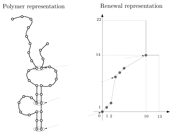
Figure 1. A configuration of the gPS model, with one strand containing 23 bases and the other 14, is represented in two fashions: the natural (or polymer) one and the renewal one. In particular we see that $(1,1)$ renewal increments (or inter-arrivals) correspond to bound base pairs and all other increments $(i,j)$ correspond to unbound regions in the bulk, that we call loops (of total length $i+j$, with length $i$ in the first strand and $j$ in the second strand). The term unbound is rather reserved to the terminal portion of the polymer: we refer the free ends as unbound strands. Throughout this work, a polymer trajectory is always given in the renewal representation: it is therefore just a point process in the plane.

In [12] it is shown that for every $h$ and every $\gamma>0$

$$\textsc{f}_{\gamma}(h):=\lim_{\begin{subarray}{c}N,M\to\infty\\ M/N\to\gamma\end{subarray}}\frac{1}{N}\log Z^{c}_{N,M,h}=\lim_{\begin{subarray}{c}N,M\to\infty\\ M/N\to\gamma\end{subarray}}\frac{1}{N}\log Z^{f}_{N,M,h}<\infty\,,$$ (1.4)

which says that the free energy (density) of free and constrained models, with binding energy $h$ and strand length asymptotic ratio equal to $\gamma$, coincide. A number of basic properties of $h\mapsto\textsc{f}_{\gamma}(h)$ are easily established, notably that it is a convex non decreasing function, equal to zero for $h\leq 0$ and positive for $h>0$. This already establishes that $h=0$ is a critical point, in the sense that $\textsc{f}_{\gamma}(\cdot)$ is not analytic at the origin.

But [12] is not limited to results on the free energy: associated to $Z^{c}_{N,M,h}$ and $Z^{f}_{N,M,h}$ there are two probability measures, that we denote respectively by ${\mathbf{P}}_{N,M,h}^{c}$ and ${\mathbf{P}}_{N,M,h}^{f}$. They are point measures, like the renewal processes on which they are built. It is standard to see that $\partial_{h}\textsc{f}_{\gamma}(h)$ (which exists except possibly for countably many values of $h$) yields the $N\to\infty$ limit of the expected density of points (under ${\mathbf{P}}_{N,M,h}^{c}$ or ${\mathbf{P}}_{N,M,h}^{f}$). Hence for $h<0$ the density is zero, while for $h>0$ the density is positive. This tells us that we are stepping from a regime in which the two strands are essentially fully unbound to a regime in which they are tightly bound. In [12] results go well beyond this: it is in particular proven that for $h<0$ the number of renewal points is $O(1)$ and these points are all close to $(0,0)$ or $(N,M)$ (see Fig. 2). In the polymer representation, this means that the two DNA strands are completely unbound, except for a few contacts between the bases just close to the extremities. More precisely, it was found in [12] that in the free case, if $\overline{\alpha}<1+\alpha/2$ the two strands are free except for $O(1)$ contacts close to the origin, and if $\overline{\alpha}>1+\alpha/2$ the two free ends are of length $O(1)$ and a large loop appears in the system, see Fig 2.

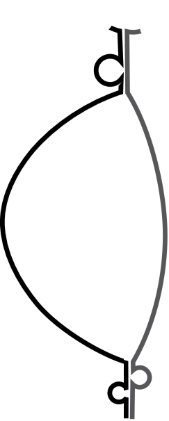
Figure 2. A schematic image of the two types of observable trajectories of the free gPS model in the delocalized (denaturated, melted) regime, according to whether the exponent $\overline{\alpha}$ is smaller (left picture) or larger (right picture) than $1+\alpha/2$. In the constrained case only the trajectory on the right is observed, and the small free tails are reduced to zero. This case is treated in [12].

On the other hand for $h>0$ the situation is radically different. This has has been analyzed in [12] but only in the Cramér regime. We are now going to discuss this in details.

1.2. Binding strategies

A way to get a grip on what is going on for $h>0$ is to observe that we can make the elementary manipulation: for every non negative $\lambda_{1}$ and $\lambda_{2}$

$$Z^{c}_{N,M,h}=e^{N\lambda_{1}+M\lambda_{2}}\sum_{n=1}^{N\wedge M}\sum_{\begin{subarray}{c}\underline{l}\in{\mathbb{N}}^{n}\\ |\underline{l}|=N\end{subarray}}\sum_{\begin{subarray}{c}\underline{t}\in{\mathbb{N}}^{n}\\ |\underline{t}|=M\end{subarray}}\prod_{i=1}^{N}\exp\left(h-\lambda_{1}l_{i}-\lambda_{2}t_{i}\right)K(l_{i}+t_{i})\,.$$ (1.5)

Since $h>0$ we identify a family, in fact a curve in $[0,\infty)^{2}$, of values of $(\lambda_{1},\lambda_{2})$ such that

$$\sum_{l,t=1}^{\infty}\exp\left(h-\lambda_{1}l-\lambda_{2}t\right)K(l+t)\,=\,1\,,$$ (1.6)

and (1.6) clearly defines a probability distribution that is an inter-arrival distribution for a new bivariate renewal process. At this point is not too difficult to get convinced that $Z^{c}_{N,M,h}$ is equal to $e^{N\lambda_{1}+M\lambda_{2}}$ times the probability that this new renewal hits $(N,M)$ (we call this probability target probability). If we are able to choose $(\lambda_{1},\lambda_{2})$ so that the logarithm of the target probability is $o(N)$, then of course $\textsc{f}_{\gamma}(h)=\lambda_{1}+\gamma\lambda_{2}$. This can actually be done: it amounts to solving a variational problem and the uniqueness of the optimal $(\lambda_{1},\lambda_{2})$ follows by convexity arguments. However the solution may be qualitatively different for different values of $h$:

1. the optimal $(\lambda_{1},\lambda_{2})$ belong to $(0,\infty)^{2}$, so both components of the inter-arrival law of the arising renewal have distributions that decay exponentially. We call this Cramér regime because the tilt of the measure (in both components) is efficient in targeting the point $(N,M)$ to which we are aiming at;

2. either $\lambda_{1}$ or $\lambda_{2}$ is zero, so only one component of the arising inter-arrival law is exponentially tight. For the sake of conciseness we call this for now non-Cramér regime because the tilt of the measure (in only one of the component) is only partially successful in targeting the point $(N,M)$. To be precise there is in reality a boundary region between the two regimes, and the notion of non-Cramér regime will be made more precise just below – this regime is the main issue of this work – so we will not dwell further on this right now.

A full treatment of the Cramér regime is given in [12], and the results can be resumed as follows: all loops are small, in fact the largest is $O(\log N)$, and the unbound strands are of length $O(1)$ – see the leftmost case in Fig 3.

In this work, we focus on the non-Cramér regime and the reader who wants to have an anticipation on the results can have a look Fig 3.

1.3. The non-Cramér regime

In order to make as explicit as possible for which values of $h>0$ the system is in the non-Cramér regime, let us define $\textsc{n}(h)>0$ as the unique solution of

$$\sum_{n,m=1}^{\infty}K(n+m)\exp\left(-n\textsc{n}(h)\right)\,=\,\exp(-h)\,.$$ (1.7)

This computation amounts to solving the variational problem we were after, in the case in which the problem is not solvable in $(0,\infty)^{2}$ and the optimal tilt of the measure involves only one of the two components. From (1.7) one can extract a number of properties of $\textsc{n}(\cdot)$: it is a real analytic, positive, convex and increasing function [12]. We insist on the fact that, in spite of being defined for every $h>0$, $\textsc{n}(h)$ is not always equal to the free energy. More precisely in [12] it is shown that $\textsc{f}_{\gamma}(h)=\textsc{n}(h)$ if and only if $\gamma\notin(1/\gamma_{c}(h),\gamma_{c}(h))$, where

$$\gamma_{c}(h)\,:=\,\frac{\sum_{n,m}mK(n+m)\exp(-n\textsc{n}(h))}{\sum_{n,m}nK(n+m)\exp(-n\textsc{n}(h))}\,.$$ (1.8)

We refer to [12] for more details on the form of the function $\gamma_{c}(\cdot)$ and the switching phenomena between the Cramér and the non-Cramér regime. In this work, and without loss of generality (by symmetry), we will consider only the case $\gamma>\gamma_{c}(h)$. To be precise we will rather consider the case $\gamma\geq\gamma_{c}(h)$ because the phenomenology observed for $\gamma>\gamma_{c}(h)$, that is for $M-\gamma_{c}(h)N\geq cN$ for some $c>0$ persists also in a part of the window $M-\gamma_{c}(h)N=o(N)$ and we will analyze the model also in this window. In different terms: the analysis in the Cramér regime is a Large Deviations analysis, but the whole non-Cramér regime is equivalent from the Large Deviations viewpoint (the issues there are about sharp deviations). So there isn’t much conceptual difference between $M-\gamma_{c}(h)N\geq cN$ and $M-\gamma_{c}(h)N=o(N)$, up to when $M-\gamma_{c}(h)N$ grows too slowly, as we shall see.

Crucial for us is the probability distribution $\hat{\mathrm{K}}_{h}(\cdot,\cdot)$ defined by

$$\hat{\mathrm{K}}_{h}(n,m)=K(n+m)e^{h-n\textsc{n}(h)}\,,$$ (1.9)

which, as announced informally just above, allows to write the partition function as

$$Z^{c}_{N,M,h}=\exp(N\textsc{n}(h)){\mathbf{P}}\left((N,M)\in\hat{\tau}_{h}\right)\,,$$ (1.10)

where $\hat{\tau}_{h}$ is the bivariate renewal process with inter-arrival distribution ${\hat{K}_{h}}(\cdot,\cdot)$. Next, we are going to have a closer look at this renewal process.

1.4. On the bivariate renewal $\hat{\tau}_{h}$

Let us write for conciseness $\textsc{n}(h)=\textsc{n}_{h}$ (a practice that we will pick up again in the proofs), and drop the dependence on $h$ in $\hat{\tau}_{h}$: $\hat{\tau}=(\hat{\tau}^{(1)},\hat{\tau}^{(2)})$. In view of (1.9), it is clear that the distribution of this process is not symmetric, we have the marginals

$$\begin{split}{\mathbf{P}}\Big{(}\hat{\tau}^{(1)}=n\Big{)}\,&=\,\sum_{m\geq 1}K(n+m)\exp(h-\textsc{n}_{h}n)\,\stackrel{{\scriptstyle n\to\infty}}{{\sim}}\,\frac{\exp(h)}{(1+\alpha)}\,\frac{L(n)}{n^{1+\alpha}}\,e^{-\textsc{n}_{h}n}\,,\\ {\mathbf{P}}\Big{(}\hat{\tau}^{(2)}=m\Big{)}\,&=\,\sum_{n\geq 1}K(n+m)\exp(h-\textsc{n}_{h}n)\,\stackrel{{\scriptstyle m\to\infty}}{{\sim}}\,\frac{\exp(h)}{\exp(\textsc{n}_{h})-1}\,\,\frac{L(m)}{m^{2+\alpha}}\,.\end{split}$$ (1.11)

Let us also denote (the dependence in $h$ is implicit)

$$\hat{\mu}_{1}:={\mathbf{E}}[\hat{\tau}^{(1)}_{1}]<+\infty,\qquad\hat{\mu}_{2}:={\mathbf{E}}[\hat{\tau}^{(2)}_{1}]<+\infty\,,$$ (1.12)

so that $\gamma_{c}(h)=\hat{\mu}_{2}/\hat{\mu}_{1}$, cf. (1.8).

We notice that the process $\hat{\tau}^{(1)}$ has moments of all orders, and so $\{\hat{\tau}^{(1)}_{n}\}_{n=0,1,\ldots}$ is in the domain of attraction of a normal law: we denote $a_{n}^{(1)}:=\sqrt{n}$ the scaling sequence for $\hat{\tau}^{(1)}_{n}$. On the other hand, the process $\{\hat{\tau}^{(2)}_{n}\}_{n=0,1,\ldots}$ is in the domain of attraction of an $\alpha_{2}$-stable law, with $\alpha_{2}:=(1+\alpha)\wedge 2>1$: its scaling sequence $a_{n}^{(2)}$ verifies

$$L(a_{n}^{(2)})(a_{n}^{(2)})^{-\alpha_{2}}\sim\,\frac{1}{n}\ \text{ if }\alpha_{2}<2\quad\quad\text{ and }\quad\quad\sigma(a_{n}^{(2)})(a_{n}^{(2)})^{-2}\sim\,\frac{1}{n}\ \text{ if }\alpha_{2}=2$$ (1.13)

where

$$\sigma(n)\,:=\,{\mathbf{E}}\Big{[}\Big{(}\hat{\tau}^{(2)}_{1}\Big{)}^{2}\mathbf{1}_{\{\hat{\tau}^{(2)}_{1}\;\leqslant\;n\}}\Big{]}\,,$$ (1.14)

and diverges as a slowly varying function if ${\mathbf{E}}[(\hat{\tau}^{(2)}_{1})^{2}]=+\infty$ (with $\sigma(n)/L(n)\to+\infty$ [3]). In particular, $a_{n}^{(2)}$ is regularly varying with exponent $1/\alpha_{2}=(1+\alpha)^{-1}\vee(1/2)$.

As an additional relevant definition, we select a sequence $\{m_{n}^{(2)}\}_{n=1,2,\ldots}$ satisfying

$${\mathbf{P}}\big{(}\hat{\tau}^{(2)}_{1}>m_{n}^{(2)}\big{)}\stackrel{{\scriptstyle n\to\infty}}{{\sim}}\frac{1}{n},$$ (1.15)

so that $m_{n}^{(2)}$ gives the order of $\max_{1\;\leqslant\;j\;\leqslant\;n}\{\hat{\tau}^{(2)}_{j}-\hat{\tau}^{(2)}_{j-1}\}$. We stress that $m_{n}^{(2)}$ is regularly varying with exponent $(1+\alpha)^{-1}$, and that $m_{n}^{(2)}/a_{n}^{(2)}\in[1/c,c]$ for some $c\geq 1$ if $\alpha<1$, but $m_{n}^{(2)}/a_{n}^{(2)}\to 0$ when $\alpha\;\geqslant\;1$: in any case, there is a constant $c>0$ such that $m_{n}^{(2)}\;\leqslant\;ca_{n}^{(2)}$ for every $n$, i.e. $m_{n}^{(2)}=O(a_{n}^{(2)})$.

Let us also stress that the bivariate renewal process $\hat{\tau}_{h}$ falls in the domain of attraction of an $(\alpha_{1}=2,\alpha_{2})$ stable distribution (see e.g. [19] or [13]). We have, as $n\to\infty$, that $\Big{\{}\Big{(}\frac{\hat{\tau}^{(1)}_{n}-\hat{\mu}_{1}n}{a_{n}^{(1)}},\frac{\hat{\tau}^{(2)}_{n}-\hat{\mu}_{2}n}{a_{n}^{(2)}}\Big{)}\Big{\}}_{n=1,2,\ldots}$ converges in distribution to $Z$, a non-degenerate $(2,\alpha_{2})$-bivariate stable law. Let us mention that in [19] it is proven that:

• If $\alpha_{2}=2$ (i.e. $\alpha\;\geqslant\;1$), then $Z$ is a bivariate normal distribution.

• If $\alpha_{2}<2$ (i.e. $\alpha\in(0,1)$), then $Z$ is a couple of independent normal and $\alpha_{2}$-stable distributions.

We mention that a bivariate local limit theorem is given in [6] and multivariate ($d$-dimensional) renewals are further studied in [2]: local large deviation estimates are given, as well as strong renewal theorems, i.e.  asymptotics of ${\mathbf{P}}((n,m)\in\tau)$ as $(n,m)\to\infty$, when $(n,m)$ is close to the favorite direction – the favorite direction exists when ${\mathbf{E}}[\tau_{1}]$ is finite and it is the line $t\mapsto t{\mathbf{E}}[\tau_{1}]$, and close to means at distance of the order of the fluctuations around that direction – we refer to [2] for further details (estimates when $(n,m)$ is away from the favorite direction are also given).

1.5. Non-Cramér regime and big-jump domain

We drop the dependence of $\gamma_{c}(h)$ on $h$, and we set

$$t_{N}\,:=M-\gamma_{c}N\,.$$ (1.16)

Of course, having $\gamma>\gamma_{c}$ means that $t_{N}/N\geq c$ for some $c>0$. But it is natural and essentially not harder to tackle the problem assuming only

$$t_{N}/a_{N}^{(2)}\to+\infty\ \text{ as }N\to\infty,$$ (1.17)

with additionally, in the case $\alpha\;\geqslant\;1$ (recall the definition of $\sigma(n)$ after (1.13))

$$\left(\frac{t_{N}}{a_{N}^{(2)}}\right)^{2}\ \frac{\sigma(a_{N})}{\sigma(t_{N})}\stackrel{{\scriptstyle N\to\infty}}{{\sim}}\frac{t_{N}^{2}}{N\sigma(t_{N})}\;\geqslant\;C_{0}\log N\ \text{ for a suitable choice of }C_{0}>0\,.$$ (1.18)

If $\alpha>1$, as well as if $\alpha=1$ and $\sigma(n)=O(1)$ (i.e. if ${\mathbf{E}}[(\hat{\tau}^{(2)}_{1})^{2}]<\infty$), (1.18) simply means that $t_{N}\;\geqslant\;C^{\prime}_{0}\sqrt{N\log N}$ with $C^{\prime}_{0}$ easily related to $C_{0}$. Note also that (1.17) implies $t_{N}\gg\sqrt{N\log N}$ if ${\mathbf{E}}[(\hat{\tau}^{(2)}_{1})^{2}]=\infty$.

We stress that the constants $C_{0}$ depends only on $K(\cdot)$ and, for the interested reader, it can be made explicit by tracking the constants in (3.33) and (3.43) where the value of $C_{0}$ is used. This assumption is made to be sure that we lie in the so called big-jump domain, as studied for example in the one-dimensional setting in [5]: in our model it simply means that deviations – and the event we focus on is $(N,M)\in\hat{\tau}$ – are realized by an atypical deviation on just one of the increment variables $\hat{\tau}_{i+1}-\hat{\tau}_{i}$. As we shall, this happens just under the assumption (1.17) for $\alpha<1$ and this condition is optimal (see Appendix B.1). For the case $\alpha\geq 1$ the extra condition (1.18) is not far from being optimal, but it is not: we discuss this point in Appendix B.2, but we do not treat it in full generality because it is a technically demanding issue that leads far from our main purposes.

1.6. Mais results I: polymer trajectories

We are now going to introduce two fundamental events in an informal, albeit precise, fashion. The two events will be rephrased in a more formal way in (2.8), once further notations will have been introduced. Choose sequences of positive numbers $\{u_{N}\}_{N=1,2,\ldots}$, $\{m^{+}_{N}\}_{N=1,2,\ldots}$, $\{a^{+}_{N}\}_{N=1,2,\ldots}$ and $\{\widetilde{a}^{+}_{N}\}_{N=1,2,\ldots}$ such that

$$u_{N}\gg 1\,,\quad t_{N}\gg m^{+}_{N}\gg m^{(2)}_{N}\,,\quad t_{N}\gg a^{+}_{N}\gg a_{N}^{(2)}\quad\text{ and }\quad t_{N}\gg\widetilde{a}^{+}_{N}\gg a_{N}^{(2)}\,.$$ (1.19)

In practice, and to optimize the result that follows, $u_{N}$, $m^{+}_{N}/m^{(2)}_{N}$, $a^{+}_{N}/a_{N}^{(2)}$ and $\widetilde{a}^{+}_{N}/a_{N}^{(2)}$ should be chosen tending to $\infty$ in an arbitrarily slow fashion.

We then define the Big Loop event $E^{(N)}_{\mathtt{BL}}$ to be the set of trajectories such that

1. there is one loop of size larger than $t_{N}-a^{+}_{N}$ and smaller than $t_{N}+a^{+}_{N}$, so that, to leading order, it is of size $t_{N}$;

2. all other loops are smaller than $m^{+}_{N}$ (hence there is only one largest loop);

3. the length of neither of the two unbound strands is larger than $u_{N}$.

The (large or macroscopic) Unbound Strand event $E^{(N)}_{\mathtt{US}}$ is instead the set of trajectories such that

1. all loops are smaller than $m^{+}_{N}$;

2. the length of the unbound portion of the shorter strand does not exceed $u_{N}$;

3. the length of the unbound portion of the longer strand is larger than $t_{N}-\widetilde{a}^{+}_{N}$ and smaller than $t_{N}+\widetilde{a}^{+}_{N}$, so that, to leading order, it is of size $t_{N}$.

Note that $E^{(N)}_{\mathtt{BL}}\cap E^{(N)}_{\mathtt{US}}=\emptyset$ except, possibly, for finitely many $N$: the two conditions (1) are incompatible. We refer to Fig. 3 for a schematic image of these two events.

Theorem 1.1.

Under assumptions (1.17), (1.18) and (1.19) we have that

$$\lim_{N\to\infty}{\mathbf{P}}^{f}_{N,M,h}\Big{(}E^{(N)}_{\mathtt{BL}}\cup E^{(N)}_{\mathtt{US}}\Big{)}\,=\,1\,.$$ (1.20)

Moreover

1. If $\overline{\alpha}<1$ (and hence $\sum_{j}K_{f}(j)=\infty$) then

   $$\lim_{N\to\infty}{\mathbf{P}}^{f}_{N,M,h}\Big{(}E^{(N)}_{\mathtt{US}}\Big{)}\,=\,1\,.$$ (1.21)

2. If $\sum_{j}K_{f}(j)<\infty$ (and hence $\overline{\alpha}\geq 1$) then

   $${\mathbf{P}}^{f}_{N,M,h}\Big{(}E^{(N)}_{\mathtt{US}}\Big{)}\stackrel{{\scriptstyle N\to\infty}}{{\sim}}\frac{1}{1+Q_{N}}\ \ \text{ and}\ \ {\mathbf{P}}^{f}_{N,M,h}\Big{(}E^{(N)}_{\mathtt{BL}}\Big{)}\stackrel{{\scriptstyle N\to\infty}}{{\sim}}\frac{Q_{N}}{1+Q_{N}}\,,$$ (1.22)

   with

   $$Q_{N}\,:=\,c_{h}N\,(t_{N})^{-(2+\alpha)+\overline{\alpha}}\,\frac{L(t_{N})}{\overline{L}(t_{N})}\ \ \text{ and }c_{h}:=\frac{e^{h}\sum_{j=0}^{\infty}K_{f}(j)}{\hat{\mu}_{1}(e^{\textsc{n}(h)}-1)}\,.$$ (1.23)

For conciseness the case $\overline{\alpha}=1$ with $\sum_{j}K_{f}(j)=+\infty$ is not included in Theorem 1.1, but its is treated in full in Appendix A. It is a marginal case in which an anomalous behavior appears: a big loop and a large unbound strand may coexist.

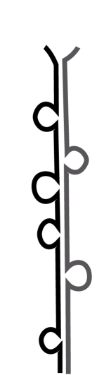
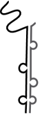
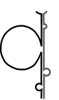
Figure 3. Schematic image of the observable trajectories of the free gPS model in the Cramér regime (left), and in the non-Cramér regime (cf. Theorem 1.1): the Large Unbound Strand event (center, occuring when $\overline{\alpha}<\alpha+1$) and the Big Loop event (right, occuring when $\overline{\alpha}>\alpha+1$). In the constrained case the Unbound Strand event is not observed, and the free tails are of course absent. What cannot be appreciated in this schematic view is the fact that the small loop distribution has exponential tail in the Cramér regime (hence the largest is $O(\log N)$) and that it has power law tail in the non-Cramér regime (hence the largest is $O(N^{a})$ for some $a\in(0,1)$: $O(m_{N})$ to be precise).

It is worth pointing out that, in most of the cases, the expressions in (1.22) have a limit – at least if $\{t_{N}\}_{N=1,2,\ldots}$ is not too wild (regularly varying is largely sufficient) – and it is either one or zero. In particular when $t_{N}\sim cN$ for some $c>0$ we have

$$\lim_{N\to\infty}{\mathbf{P}}^{f}_{N,M,h}\left(E^{(N)}_{\mathtt{US}}\right)\,=\,\begin{cases}1&\mathrm{if}\ \overline{\alpha}<\alpha+1\ \mathrm{or\ if}\ \overline{\alpha}=\alpha+1\ \mathrm{and}\ \overline{L}(t)\stackrel{{\scriptstyle t\to\infty}}{{\gg}}L(t),\\ 0&\mathrm{if}\ \overline{\alpha}>\alpha+1\ \mathrm{or\ if}\ \overline{\alpha}=\alpha+1\ \mathrm{and}\ \overline{L}(t)\stackrel{{\scriptstyle t\to\infty}}{{\ll}}L(t).\\ \end{cases}$$ (1.24)

(This is true also in the case $\overline{\alpha}=1$ with $\sum_{j}K_{f}(j)=+\infty$, see (A.6)-(A.7)). Note that in the case in which $\overline{\alpha}=\alpha+1$ and the ratio of the two slowly varying function has a limit which is neither $0$ nor $\infty$, the limit of the probability of the unbound strand event exists and it is an explicit value in $(0,1)$.

2. Main results II: sharp estimates on the partition functions

In this section, we give the asymptotic behavior of $e^{-N\textsc{n}_{h}}Z_{N,M,h}^{c}={\mathbf{P}}((N,M)\in\hat{\tau})$ in the big-jump domain. Then we present the asymptotic behavior of $Z_{N,M,h}^{f}$. Both in the constrained and free case we also give more technical estimates that identify some events to which we can restrict the partition functions without modifying them in a relevant way. Theorem 1.1 turns out to be a corollary of these technical estimates, as we explain in the final part of the section.

In this section and in the rest of the paper we deal with order statistics and we introduce here the relative definitions. Consider the (non-increasing) order statistics $\big{\{}\mathcal{M}_{1,k},\mathcal{M}_{2,k},\ldots,\mathcal{M}_{k,k}\big{\}}$ of the IID family $\{\hat{\tau}^{(2)}_{j}-\hat{\tau}^{(2)}_{j-1}\}_{j=1,\ldots,k}$. In particular $\mathcal{M}_{1,k}$ is a maximum of this finite sequence. We will consider the order statistics also for $k$ random, notably for $k=\kappa_{N}:=\max\{i\,:\,\hat{\tau}^{(1)}_{i}\in[0,N]\}$.

2.1. On the constrained partition function

We start with an important estimate for the constrained partition function (more precisely for the renewal mass function ${\mathbf{P}}((N,M)\in\hat{\tau})$), that is essential for the study of the free partition function, as one can imagine from its definition (1.3). It is worth insisting on the link between ${\mathbf{P}}$ and the measure we are interested in for the constrained case:

$${\mathbf{P}}_{N,M,h}^{c}(\cdot)\,=\,{\mathbf{P}}(\,\cdot\,|(N,M)\in\hat{\tau})\,.$$ (2.1)

Theorem 2.1.

Assume that $\alpha>0$ and (1.17). Moreover if $\alpha\;\geqslant\;1$ assume also (1.18). Then (recall that $M=\gamma_{c}N+t_{N}$) we have that

$${\mathbf{P}}\big{(}(N,M)\in\hat{\tau}\big{)}={\mathbf{P}}\Big{(}\hat{\tau}^{(1)}_{\kappa_{N}}=N,\,\hat{\tau}^{(2)}_{\kappa_{N}}=M\Big{)}\stackrel{{\scriptstyle N\to\infty}}{{\sim}}\frac{N}{\hat{\mu}_{1}^{2}}{\mathbf{P}}\Big{(}\hat{\tau}^{(2)}_{1}=\lceil t_{N}\rceil\Big{)}.$$ (2.2)

Moreover, for every $\eta\in(0,1)$ there exist $\varepsilon_{0}>0$ such that for every $\varepsilon\in(0,\varepsilon_{0})$ and $N$ sufficiently large (how large may depend on $\varepsilon$), we have

$${\mathbf{P}}\bigg{(}\mathcal{M}_{1,\kappa_{N}}-t_{N}\in\Big{[}-\frac{a_{N}^{(2)}}{\varepsilon},\frac{a_{N}^{(2)}}{\varepsilon}\Big{]},\,\mathcal{M}_{2,\kappa_{N}}\leq\frac{m_{N}^{(2)}}{\varepsilon},\,\hat{\tau}^{(1)}_{\kappa_{N}}=N,\,\hat{\tau}^{(2)}_{\kappa_{N}}=M\bigg{)}\,\geq\\ \geq(1-\eta)\frac{N}{\hat{\mu}_{1}^{2}}{\mathbf{P}}\Big{(}\hat{\tau}^{(2)}_{1}=\lceil t_{N}\rceil\Big{)}\,.$$ (2.3)

2.2. On the free partition function

We now give the behavior of the free partition function and identify trajectories contributing the most to it. Let us introduce some notations:

$$V_{1}^{(N)}:=N-\hat{\tau}^{(1)}_{\kappa_{N}},\qquad V_{2}^{(N)}:=M-\hat{\tau}^{(2)}_{\kappa_{N}}\,,$$ (2.4)

the lengths of the free parts, see Fig 1.

For a set $A$ of allowed trajectories, we define $Z_{N,M,h}^{f}(A)$ the partition function restricted to trajectories in $A$ (by restricting the summation over subsets of $\{1,\ldots N\}\times\{1,\ldots M\}$ to those in $A$). For example, $Z_{N,M,h}^{f}((N,M)\in\hat{\tau})=Z_{N,M,h}^{c}$.

We set $\overline{K}:=\sum_{j=1}^{\infty}K_{f}(j)$ if the sum is finite, and we set $\overline{K}=0$ if $\sum_{j}K_{f}(j)=+\infty$.

Theorem 2.2.

Assume that $\alpha>0$ and (1.17). Moreover if $\alpha\;\geqslant\;1$ assume also (1.18) and if $\overline{\alpha}=1$ assume that $\sum_{j}K_{f}(j)<\infty$. Then for $N\to\infty$

$$e^{-N\textsc{n}(h)}Z_{N,M,h}^{f}=(1+o(1))\overline{K}\,\frac{N}{\hat{\mu}_{1}^{2}}\bigg{(}\sum_{i\geq 0}K_{f}(i)e^{-i\textsc{n}(h)}\bigg{)}{\mathbf{P}}\Big{(}\hat{\tau}^{(2)}_{1}=\lceil t_{N}\rceil\Big{)}\\ +(1+o(1))\frac{1}{\hat{\mu}_{1}}\bigg{(}\sum_{i\;\geqslant\;0}K_{f}(i)e^{-i\textsc{n}_{h}}\bigg{)}K_{f}\left(t_{N}\right)\,.$$ (2.5)

Moreover, for every $\eta\in(0,1)$ there exist $\varepsilon_{0}>0$ such that for every $\varepsilon\in(0,\varepsilon_{0})$ and $N$ sufficiently large (how large may depend on $\varepsilon$), such that

$$e^{-N\textsc{n}_{h}}Z_{N,M,h}^{f}\bigg{(}V_{1}^{(N)},V_{2}^{(N)}\;\leqslant\;\frac{1}{\varepsilon},\, \mathcal{M}_{1,\kappa_{N}}\in\Big{[}t_{N}-\frac{a_{N}^{(2)}}{\varepsilon},t_{N}+\frac{a_{N}^{(2)}}{\varepsilon}\Big{]},\,\mathcal{M}_{2,\kappa_{N}}\leq\frac{m_{N}^{(2)}}{\varepsilon}\bigg{)}$$

$$\;\geqslant\;(1-\eta)\overline{K}\,\frac{N}{\hat{\mu}_{1}^{2}}\bigg{(}\sum_{i\;\geqslant\;0}K_{f}(i)e^{-i\textsc{n}_{h}}\bigg{)}{\mathbf{P}}\left(\hat{\tau}^{(2)}_{1}=t_{N}\right)\,;$$ (2.6)

$$e^{-N\textsc{n}_{h}}Z_{N,M,h}^{f}\bigg{(}V_{1}^{(N)}\;\leqslant\;\frac{1}{\varepsilon},V_{2}^{(N)} \in\Big{[}t_{N}-\frac{a_{N}^{(2)}}{\varepsilon},t_{N}+\frac{a_{N}^{(2)}}{\varepsilon}\Big{]},\mathcal{M}_{1,\kappa_{N}}\;\leqslant\;\frac{m_{N}^{(2)}}{\varepsilon}\bigg{)}$$

$$\;\geqslant\;(1-\eta)\frac{1}{\hat{\mu}_{1}}\bigg{(}\sum_{i\;\geqslant\;0}K_{f}(i)e^{-i\textsc{n}_{h}}\bigg{)}K_{f}\left(t_{N}\right)\,.$$ (2.7)

We remark that when $\overline{\alpha}<1$, that is $\overline{K}=0$, the right-hand side of (2.5) reduces to one term and (2.6) becomes trivial. The case $\overline{\alpha}=1$ with $\sum_{j}K_{f}(j)=+\infty$ is treated in Theorem A.1.

2.3. Back to the Big Loop and Unbound Strand events.

The notations we have introduced allow a compact formulation of the two key events of Theorem 1.1:

$$\begin{split}E^{(N)}_{\mathtt{BL}}\,&=\,\left\{\mathcal{M}_{1,\kappa_{N}}\in[t_{N}-a_{N}^{+},t_{N}+a_{N}^{+}],\,\mathcal{M}_{2,\kappa_{N}}<m^{+}_{N},\,\max\left(V_{1}^{(N)},V_{2}^{(N)}\right)\leq u_{N}\right\}\,,\\ E^{(N)}_{\mathtt{US}}\,&=\,\left\{\mathcal{M}_{1,\kappa_{N}}<m^{+}_{N},\,V_{1}^{(N)}\leq u_{N},\,V_{2}^{(N)}\in[t_{N}-\widetilde{a}_{N}^{+},t_{N}+\widetilde{a}_{N}^{+}]\right\}\,.\end{split}$$ (2.8)

Proof of Theorem 1.1. This is just a book-keeping exercise using the three estimates in Theorem 2.2, together with the definition of $K_{f}(t_{N})$ and the estimate of ${\mathbf{P}}(\hat{\tau}^{(2)}_{1}=\lceil t_{N}\rceil)$ in (1.11). ∎

Finally, in the same way, we obtain from Theorem 2.1 the following complement to Theorem 1.1 for the constrained case.

Theorem 2.3.

Under assumptions (1.17) (and additionally (1.18) if $\alpha\geq 1$) and (1.19) we have that

$$\lim_{N\to\infty}{\mathbf{P}}^{c}_{N,M,h}\left(E^{(N)}_{\mathtt{BL},0}\right)\,=\,1\,,$$ (2.9)

where $E^{(N)}_{\mathtt{BL},0}$ is the event $E^{(N)}_{\mathtt{BL}}$ with the more stringent condition that $\max(V_{1}^{(N)},V_{2}^{(N)})=0$.

2.4. A word about the arguments of proof and organization of the remaining sections

As we pointed out at the beginning of the introduction, condensation phenomena are widely studied in the mathematical literature (see [5, 1] and references therein), but not in the multivariate context. The full multivariate context is the object of [2], where renewal estimates ${\mathbf{P}}((n_{1},\ldots,n_{d})\in\hat{\tau})$ are given: in particular, in the big-jump domain, only rough (general) bounds are given. Here, we address only the special bivariate case motivated by the application so that we are able to give the exact asymptotic behavior. One of the main difficulties we face is that, on the event $(N,M)\in\hat{\tau}$, the number $\kappa_{N}$ of renewal points is random and highly constrained by this event. We show that in the big-jump domain considered in Section 1.5, the main contribution to the probability ${\mathbf{P}}((N,M)\in\hat{\tau})$ comes from trajectories with a number of renewal points that is approximately $k_{N}=N/\hat{\mu}_{1}+O(\sqrt{N})$. For this number $k_{N}$, $\hat{\tau}^{(1)}_{k_{N}}$ does not have to deviate from its typical behavior to be equal to $N$, but $\hat{\tau}_{k_{N}}^{(2)}$ has to deviate from its typical behavior to reach $M$ and it does so by making one single big jump, of order $t_{N}+O(a_{N}^{(2)})$. In this sense, if we accept that $\kappa_{N}$ is forced to be $N/\hat{\mu}_{1}+O(\sqrt{N})$ by the condition $N\in\hat{\tau}^{(1)}$, we can focus on $M\in\hat{\tau}^{(2)}$ and the problem becomes almost one dimensional. This turns out to be a lower bound strategy: for a corresponding upper bound we have to show that all other trajectories bring a negligible contribution to ${\mathbf{P}}((N,M)\in\hat{\tau})$.

In the rest of the paper, we estimate separately the constrained and free partition functions. We deal with the constrained partition function in Section 3: the main term (2.3) in Section 3.1 and the remaining negligible contributions in Section 3.2. The free partition function is dealt with in Section 4: the main terms (2.6) and (2.7) in Section 4.1 and the remaining negligible contributions in Section 4.2. In Appendix A we complete the analysis of the case $\overline{\alpha}=1$. In Appendix B we discuss the transition from the big-jump regime (a single big jump, with a big deviation of just one of the two components) to the Cramér deviation strategy (no big jump).

To keep things simpler in the rest of the paper, and with some abuse of notation, we will systematically omit the integer part in the formulas.

3. The constrained partition function: proof of Theorem 2.1

3.1. Proof of the lower bound (2.3)

We start by decomposing the event of interest according to $\kappa_{N}=k$. The probability of such an event, restricted to $\{\kappa_{N}=k\}$, becomes (recall that $M=\gamma_{c}N+t_{N}$)

$${\mathbf{P}}\Big{(}\mathcal{M}_{1,k}\geq t_{N}-\frac{a_{N}^{(2)}}{\varepsilon},\,\mathcal{M}_{2,k}\leq\frac{m_{N}^{(2)}}{\varepsilon},\,\hat{\tau}^{(1)}_{k}=N,\,\hat{\tau}^{(2)}_{k}=M\Big{)}\,=\\ {\mathbf{P}}\bigg{(}\bigcup_{j=1}^{k}\Big{\{}\hat{\tau}^{(2)}_{j}-\hat{\tau}^{(2)}_{j-1}\in t_{N}+I_{N},\,\max_{i\neq j}\left(\hat{\tau}^{(2)}_{i}-\hat{\tau}^{(2)}_{i-1}\right)\leq\frac{m_{N}^{(2)}}{\varepsilon},\,\hat{\tau}^{(1)}_{k}=N,\,\hat{\tau}^{(2)}_{k}=M\Big{\}}\bigg{)}\,,$$ (3.1)

where we defined $I_{N}:=\{-a_{N}^{(2)}/\varepsilon,\ldots,a_{N}^{(2)}/\varepsilon\}$. Since $t_{N}-a_{N}^{(2)}/\varepsilon$ is larger than ${m_{N}^{(2)}}/{\varepsilon}$ (recall that $m_{n}^{(2)}\;\leqslant\;ca_{n}^{(2)}$ for every $n$ and (1.18)) for $N$ sufficiently large, the union in the right-hand side of (3.1) is a union of disjoint events that have all the same probability. This term is equal to

$$k\,{\mathbf{P}}\Big{(}\hat{\tau}^{(2)}_{1}\in t_{N}+I_{N},\,\max_{i=2,\ldots,k}\left(\hat{\tau}^{(2)}_{i}-\hat{\tau}^{(2)}_{i-1}\right)\leq\frac{m_{N}^{(2)}}{\varepsilon},\,\hat{\tau}^{(1)}_{k}=N,\,\hat{\tau}^{(2)}_{k}=\gamma_{c}N+t_{N}\Big{)}\,=\\ k\,\sum_{y\in I_{N}}\sum_{x\in{\mathbb{N}}}{\mathbf{P}}\Big{(}\hat{\tau}^{(2)}_{1}=t_{N}+y,\,\hat{\tau}^{(1)}_{1}=x\Big{)}{\mathbf{P}}\Big{(}\mathcal{M}_{1,k-1}\;\leqslant\;\frac{m_{N}^{(2)}}{\varepsilon},\hat{\tau}^{(1)}_{k-1}=N-x,\,\hat{\tau}^{(2)}_{k-1}=\gamma_{c}N-y\Big{)}\,,$$ (3.2)

where we have used that $\{(\hat{\tau}^{(1)}_{j}-\hat{\tau}^{(1)}_{1},\hat{\tau}^{(2)}_{j}-\hat{\tau}^{(2)}_{1})\}_{j=2,\ldots,k}$ and $\{(\hat{\tau}^{(1)}_{j},\hat{\tau}^{(2)}_{j})\}_{j=1,\ldots,k-1}$ have the same law.

Since we are after a lower bound we may and do restrict the sum over $x$ between $1$ and $1/\varepsilon$ and $y\in I_{N}:=\{-a_{N}^{(2)}/\varepsilon,\ldots,a_{N}^{(2)}/\varepsilon\}$. And using that ${\mathbf{P}}(\hat{\tau}^{(2)}_{1}=n)$ is regularly varying, we have that uniformly for such $x$ and $y\in I_{N}$

$${\mathbf{P}}\Big{(}\hat{\tau}^{(2)}_{1}=t_{N}+y,\,\hat{\tau}^{(1)}_{1}=x\Big{)}\,\geq\left(1-\delta_{N}\right){\mathbf{P}}\Big{(}\hat{\tau}^{(2)}_{1}=t_{N}\Big{)}\widetilde{\mathbf{P}}\Big{(}\hat{\tau}^{(1)}_{1}=x\,\Big{|}\,\hat{\tau}^{(2)}_{1}=t_{N}+y\Big{)}\,,$$

where $\delta_{N}=\delta_{N}(\varepsilon)\geq 0$ is such that $\lim_{N\to\infty}\delta_{N}=0$. If now we set $p_{h}(x):=(e^{\textsc{n}_{h}}-1)e^{-x\textsc{n}_{h}}$, by using (1.11) we have that

$$\begin{split}{\mathbf{P}}\Big{(}\hat{\tau}^{(1)}_{1}=x\,\big{|}\,\hat{\tau}^{(2)}_{1}=&t_{N}+y\Big{)}\,=\,\frac{{\mathbf{P}}\big{(}\hat{\tau}^{(1)}_{1}=x,\,\hat{\tau}^{(2)}_{1}=t_{N}+y\big{)}}{{\mathbf{P}}\big{(}\hat{\tau}^{(2)}_{1}=t_{N}+y\big{)}}\\ &\geq\,\left(1-\delta_{N}\right)\frac{p_{h}(x)K\left(t_{N}+x+y\right)}{K\left(t_{N}+y\right)}\,\geq\,\left(1-\delta_{N}\right)^{2}p_{h}(x)\,,\end{split}$$ (3.3)

possibly for a different choice of $\delta_{N}=\delta_{N}(\varepsilon)$. Therefore, going back to (3.1) we see that (again, by redefining $\delta_{N}$)

$${\mathbf{P}}\Big{(}\mathcal{M}_{1,k}\in t_{N}+I_{N},\,\mathcal{M}_{2,k}\leq\frac{m_{N}^{(2)}}{\varepsilon},\,\hat{\tau}^{(1)}_{k}=N,\,\hat{\tau}^{(2)}_{k}=M\Big{)}\,\geq\\ (1-\delta_{N})k\,{\mathbf{P}}\big{(}\hat{\tau}^{(2)}_{1}=t_{N}\big{)}\sum_{x=1}^{1/\varepsilon}p_{h}(x){\mathbf{P}}\Big{(}\mathcal{M}_{1,k-1}\;\leqslant\;\frac{m_{N}^{(2)}}{\varepsilon},\hat{\tau}^{(1)}_{k-1}=N-x,\,\hat{\tau}^{(2)}_{k-1}-\gamma_{c}N\in I_{N}\Big{)}\,.$$ (3.4)

We now sum over the values of $k$ and we restrict to $k\in[(N/\hat{\mu}_{1})-\sqrt{N/\varepsilon},(N/\hat{\mu}_{1})+\sqrt{N/\varepsilon}]\cap{\mathbb{Z}}:=J_{N}$. Hence, redefining $\delta_{N}$, the left-hand side of (2.3) is bounded from below by

$$(1-\delta_{N}){\mathbf{P}}\Big{(}\hat{\tau}^{(2)}_{1}=t_{N}\Big{)}\frac{N}{\hat{\mu}_{1}}\sum_{x=1}^{1/\varepsilon}p_{h}(x)P_{\varepsilon}(x)\,,$$ (3.5)

where we defined, with $n_{N}^{+}:=\max J_{N}$,

$$P_{\varepsilon}(x):=\sum_{k\in J_{N}}{\mathbf{P}}\bigg{(}\max_{i=1,\ldots,n^{+}_{N}}\left(\hat{\tau}^{(2)}_{i}-\hat{\tau}^{(2)}_{i-1}\right)\;\leqslant\;\frac{m_{N}^{(2)}}{\varepsilon},\hat{\tau}^{(1)}_{k-1}=N-x,\,\hat{\tau}^{(2)}_{k-1}-\gamma_{c}N\in I_{N}\bigg{)}$$ (3.6)

For $P_{\varepsilon}(x)$, we observe right away that by introducing also $n^{-}_{N}:=\min J_{N}$ – note that $n_{N}^{\pm}$ are equal to $(N/\hat{\mu}_{1})\pm\sqrt{N/\varepsilon}$ – we have

$$\begin{split}P_{\varepsilon}(x)\,\geq\,&\sum_{k\in J_{N}}{\mathbf{P}}\bigg{(}\mathcal{M}_{1,n^{+}_{N}}\;\leqslant\;\frac{m_{N}^{(2)}}{\varepsilon},\hat{\tau}^{(1)}_{k-1}=N-x\bigg{)}\\ &-\sum_{k\in J_{N}}{\mathbf{P}}\bigg{(}\mathcal{M}_{1,n^{+}_{N}}\;\leqslant\;\frac{m_{N}^{(2)}}{\varepsilon},\hat{\tau}^{(1)}_{k-1}=N-x,\,\hat{\tau}^{(2)}_{n^{+}_{N}}-\gamma_{c}N>\frac{a_{N}^{(2)}}{\varepsilon}\bigg{)}\\ &-\sum_{k\in J_{N}}{\mathbf{P}}\bigg{(}\mathcal{M}_{1,n^{+}_{N}}\;\leqslant\;\frac{m_{N}^{(2)}}{\varepsilon},\hat{\tau}^{(1)}_{k-1}=N-x,\,\hat{\tau}^{(2)}_{n^{-}_{N}}-\gamma_{c}N<\frac{a_{N}^{(2)}}{\varepsilon}\bigg{)}\\ &\;\geqslant\;{\mathbf{P}}\left(E_{1}\cap E_{2}(x)\right)-{\mathbf{P}}\left(E^{+}_{3}\right)-{\mathbf{P}}\left(E^{-}_{3}\right)\,,\end{split}$$ (3.7)

where

$$E_{1}\,:=\,\Big{\{}\mathcal{M}_{1,n^{+}_{N}}\;\leqslant\;\frac{m_{N}^{(2)}}{\varepsilon}\Big{\}}\,,\qquad E_{2}(x)\,:=\,\left\{\exists k\in J_{N}\textrm{ such that }\hat{\tau}^{(1)}_{k-1}=N-x\right\}\,,$$ (3.8)

and

$$E_{3}^{+}\,:=\,\Big{\{}\hat{\tau}^{(2)}_{n^{+}_{N}}-\gamma_{c}N>\frac{a_{N}^{(2)}}{\varepsilon}\Big{\}}\,,\qquad E_{3}^{-}\,:=\,\Big{\{}\hat{\tau}^{(2)}_{n^{-}_{N}}-\gamma_{c}N<\frac{a_{N}^{(2)}}{\varepsilon}\Big{\}}\,.$$ (3.9)

We now estimate separately the probability of these events.

$E_{1}$ has probability close to one

For this, we use that ${\mathbf{P}}(\hat{\tau}^{(2)}_{1}>n)$ is regularly varying with index $(1+\alpha)^{-1}$ together with the definition (1.15) of $m_{n}^{(2)}$ to obtain that for $N$ larger than some constant $N_{0}=N_{0}(\varepsilon)$ we have ${\mathbf{P}}\left(\hat{\tau}^{(2)}_{1}>\tfrac{1}{\varepsilon}m_{N}^{(2)}\right)\;\leqslant\;2\varepsilon^{1+\alpha}N^{-1}$. Therefore, we have for $N\;\geqslant\;N_{0}$

$${\mathbf{P}}\left(E_{1}\right)\,\;\geqslant\;\,\left(1-2\varepsilon^{1+\alpha}N^{-1}\right)^{n^{+}_{N}}\;\geqslant\;e^{-3\varepsilon^{1+\alpha}}\,.$$ (3.10)

where we used that $n_{N}^{+}\;\leqslant\;N$ and $\varepsilon$ small.

$E_{2}(x)$ has probability close to $1/\hat{\mu}_{1}$

The probability of $E_{2}(x)$ is estimated by writing

$$\begin{split}{\mathbf{P}}\left(E_{2}(x)\right)\,&={\mathbf{P}}(N-x\in\hat{\tau}^{(1)})-\sum_{k<n_{N}^{-}}{\mathbf{P}}\left(\hat{\tau}^{(1)}_{k}=N-x\right)-\sum_{k>n_{N}^{+}}{\mathbf{P}}\left(\hat{\tau}^{(1)}_{k}=N-x\right)\\ &\;\geqslant\;{\mathbf{P}}(N-x\in\hat{\tau}^{(1)})-{\mathbf{P}}\Big{(}\hat{\tau}^{(1)}_{n_{N}^{-}}\;\geqslant\;N-\tfrac{1}{\varepsilon}\Big{)}-{\mathbf{P}}\Big{(}\hat{\tau}^{(1)}_{n_{N}^{+}}\;\leqslant\;N\Big{)}\,,\end{split}$$ (3.11)

where for the second term we used that ${\mathbf{P}}\big{(}\exists\,k<n_{N}^{-}\text{ s.t. }\hat{\tau}^{(1)}_{k}=N-x\big{)}\;\leqslant\;{\mathbf{P}}\big{(}\hat{\tau}^{(1)}_{n_{N}^{-}}\;\geqslant\;N-x\big{)}$ together with the fact that $x\;\leqslant\;1/\varepsilon$ (and similarly for the last term).

First, because the inter-arrivals of $\hat{\tau}^{(1)}$ are exponentially integrable, $|{\mathbf{P}}(N\in\hat{\tau}^{(1)})-1/\hat{\mu}_{1}|\leq\exp(-cN)$ for $N\geq N_{0}$ with $c>0$ and $N_{0}$ that depend on the inter-arrival law [15]. Therefore, uniformly in $x=1,\ldots,1/\varepsilon$, we have that for $N$ sufficiently large ${\mathbf{P}}(N-x\in\hat{\tau}^{(1)})\;\geqslant\;1/\hat{\mu}_{1}-e^{-cN/2}$.

For the remaining terms in (3.11) it is just a matter of using the Central Limit Theorem. In fact, recalling that $n_{N}^{-}=N/\hat{\mu}_{1}-\sqrt{N/\varepsilon}$, we have

$${\mathbf{P}}\Big{(}\hat{\tau}^{(1)}_{n_{N}^{-}}\;\geqslant\;N-\tfrac{1}{\varepsilon}\Big{)}={\mathbf{P}}\Big{(}\hat{\tau}^{(1)}_{n_{N}^{-}}-\hat{\mu}_{1}n_{N}^{-}\;\geqslant\;\hat{\mu}_{1}\varepsilon^{-1/2}\sqrt{N}-\tfrac{1}{\varepsilon}\Big{)}\;\leqslant\;e^{-c\varepsilon^{-1}},$$ (3.12)

for $N$ larger than some $N_{0}=N_{0}(\varepsilon)$. On the other hand, we also have that

$${\mathbf{P}}\Big{(}\hat{\tau}^{(1)}_{n_{N}^{+}}\;\leqslant\;N\Big{)}={\mathbf{P}}\Big{(}\hat{\tau}^{(1)}_{n_{N}^{+}}-\hat{\mu}_{1}n_{N}^{+}\;\leqslant\;-\hat{\mu}_{1}\varepsilon^{-1/2}\sqrt{N}\Big{)}\;\leqslant\;e^{-c^{\prime}\varepsilon^{-1}},$$ (3.13)

provided again that $N$ is large enough.

Therefore we have proven that for every $\eta\in(0,1)$ there exists $\varepsilon_{0}$ and $N_{0}:(0,1)\to{\mathbb{N}}$ such that for $\varepsilon\in(0,\varepsilon_{0})$ and $N\geq N_{0}(\varepsilon)$ we have

$$\min_{x=1,\ldots,1/\varepsilon}{\mathbf{P}}\left(E_{2}(x)\right)\,\geq\,\frac{1-\eta}{\hat{\mu}_{1}}\,.$$ (3.14)

$E_{3}^{\pm}$ have a small probability

This is a consequence of the convergence to stable limit law. In fact, using that $\gamma_{c}=\hat{\mu}_{2}/\hat{\mu}_{1}$ so that $\gamma_{c}N=\hat{\mu}_{2}n_{N}^{+}-\hat{\mu}_{2}\sqrt{N/\varepsilon}$, we get

$$E_{3}^{+}\,=\bigg{\{}\hat{\tau}^{(2)}_{n^{+}_{N}}-\hat{\mu}_{2}n^{+}_{N}\,>\,\frac{a_{N}^{(2)}}{\varepsilon}-\hat{\mu}_{2}\sqrt{N/\varepsilon}\bigg{\}}\subset\bigg{\{}\hat{\tau}^{(2)}_{n^{+}_{N}}-\hat{\mu}_{2}n^{+}_{N}\,>\,\frac{a_{N}^{(2)}}{2\varepsilon}\bigg{\}}\,,$$ (3.15)

where the last inclusion holds provided that $\varepsilon$ is sufficiently small, since there is a constant $c$ such that $a_{N}^{(2)}\;\geqslant\;c\sqrt{N}$ for all $N$ (we actually simply need $N$ to be large if $a_{N}^{(2)}/\sqrt{N}\to+\infty$ for $N\to\infty$, which is the case when ${\mathbf{E}}[(\hat{\tau}^{(2)}_{1})^{2}]=+\infty$). Very much in the same way we get also to

$$E_{3}^{-}\,\subset\,\bigg{\{}\hat{\tau}^{(2)}_{n^{-}_{N}}-\hat{\mu}_{2}n^{-}_{N}\,<\,-\frac{a_{N}^{(2)}}{2\varepsilon}\bigg{\}}\,.$$ (3.16)

Since $(\hat{\tau}^{(2)}_{n^{\pm}_{N}}-\hat{\mu}_{2}n^{\pm}_{N})/a_{n^{\pm}_{N}}^{(2)}$ converges in law for $N\to\infty$ to a stable limit variable $Y$, and using that $a_{N}^{(2)}/a^{(2)}_{n_{N}^{\pm}}\to\hat{\mu}_{1}^{1/\alpha_{2}}$ (since $n_{N}^{\pm}\sim N/\mu_{1}$ and $a_{N}^{(2)}$ is regularly varying with exponent $\alpha_{2}^{-1}$, recall $\alpha_{2}:=\min(1+\alpha,2)$), it is straightforward to see that

$$\limsup_{N\to\infty}{\mathbf{P}}(E_{3}^{+})\,\leq\,{\mathbf{P}}\bigg{(}Y\geq\frac{\hat{\mu}_{1}^{1/\alpha_{2}}}{2\varepsilon}\bigg{)}\ \text{ and }\ \limsup_{N\to\infty}{\mathbf{P}}(E_{3}^{-})\,\leq\,{\mathbf{P}}\bigg{(}Y\leq-\frac{\hat{\mu}_{1}^{1/\alpha_{2}}}{2\varepsilon}\bigg{)}\,,$$ (3.17)

which are both vanishing as $\varepsilon\searrow 0$.

We therefore see that (3.10), (3.14) and (3.17) yield that, provided that $\varepsilon_{0}$ is small enough, for every $\varepsilon<\varepsilon_{0}$ and $N$ large enough (how large depends on $\varepsilon$), $P_{\varepsilon}(x)\;\geqslant\;(1-\eta)/\mu_{1}$ uniformly for $x\in\{1,\ldots,1/\varepsilon\}$. If we now go back to (3.5) and (3.7), and using that $\sum_{x\;\geqslant\;1}p_{h}(x)=1$, we obtain(2.3). ∎

3.2. Proof of (2.2)

In view of (2.3), we simply need to give an upper bound on the probability ${\mathbf{P}}\left((N,\gamma_{c}N+t_{N})\in\hat{\tau}\right)$. Fix some $\varepsilon>0$.

First step. We control

$${\mathbf{P}} \Big{(}\mathcal{M}_{1,\kappa_{N}}>(1-\varepsilon)t_{N},\hat{\tau}^{(1)}_{\kappa_{N}}=N,\hat{\tau}^{(2)}_{\kappa_{N}}=\gamma_{c}N+t_{N}\Big{)}$$

$$\leq\sum_{k=1}^{N}k\sum_{y>-\varepsilon t_{N}}\sum_{x\in{\mathbb{N}}}{\mathbf{P}}\left(\hat{\tau}^{(2)}_{1}=t_{N}+y,\,\hat{\tau}^{(1)}_{1}=x\right){\mathbf{P}}\left(\hat{\tau}^{(1)}_{k-1}=N-x,\hat{\tau}^{(2)}_{k-1}=\gamma_{c}N-y\right)\,.$$ (3.18)

Recalling (1.9) and (1.11), we have that there is some $N_{0}=N_{0}(\varepsilon)$ and some $\eta=\eta_{\varepsilon}$ (with $\eta_{\varepsilon}\to 0$ as $\varepsilon\downarrow 0$), such that for all $N\;\geqslant\;N_{0}$, $x\;\leqslant\;1/\varepsilon$ and $y>-\varepsilon t_{N}$ we have

$${\mathbf{P}}\Big{(}\hat{\tau}^{(2)}_{1}=t_{N}+y,\,\hat{\tau}^{(1)}_{1}=x\Big{)}=\frac{L\left(t_{N}+y+\right)}{\left(t_{N}+y+x\right)^{2+\alpha}}e^{h-x\textsc{n}_{h}}\;\leqslant\;(1+\eta){\mathbf{P}}\Big{(}\hat{\tau}^{(2)}_{1}=t_{N}\Big{)}p_{h}(x),$$ (3.19)

where we recall that $p_{h}(x):=(e^{\textsc{n}_{h}}-1)e^{-x\textsc{n}_{h}}$. Note that we also have that there is a constant $c$ such that uniformly for $x\in{\mathbb{N}}$

$${\mathbf{P}}\Big{(}\hat{\tau}^{(2)}_{1}=z,\,\hat{\tau}^{(1)}_{1}=x\Big{)}\;\leqslant\;cL(z)z^{-(2+\alpha)}p_{h}(x)\,.$$ (3.20)

We can use that to get that uniformly for $y\;\geqslant\;-t_{N}/2$ (so that $t_{N}+y\;\geqslant\;t_{N}/2$) we have that for any $x\;\geqslant\;1$

$${\mathbf{P}}\Big{(}\hat{\tau}^{(2)}_{1}=t_{N}+y,\,\hat{\tau}^{(1)}_{1}=x\Big{)}\;\leqslant\;c^{\prime}p_{h}(x){\mathbf{P}}\Big{(}\hat{\tau}^{(2)}_{1}=t_{N}\Big{)}.$$ (3.21)

Then, dividing (3.18) according to whether $x\leq 1/\varepsilon$ or $x>1/\varepsilon$ (and summing over $y>\varepsilon t_{N}$), we obtain the following upper bound

$$(1+\eta)\sum_{x=1}^{1/\varepsilon}p_{h}(x){\mathbf{P}}\Big{(}\hat{\tau}^{(2)}_{1}=t_{N}\Big{)}\sum_{k=1}^{N}k{\mathbf{P}}\Big{(}\hat{\tau}^{(1)}_{k-1}=N-x\Big{)}\\ +c\sum_{x=1/\varepsilon}^{N}p_{h}(x){\mathbf{P}}\Big{(}\hat{\tau}^{(2)}_{1}=t_{N}\Big{)}\sum_{k=1}^{N}k{\mathbf{P}}\Big{(}\hat{\tau}^{(1)}_{k-1}=N-x\Big{)}\,.$$ (3.22)

The second term is bounded from above by

$$cN{\mathbf{P}}\Big{(}\hat{\tau}^{(2)}_{1}=t_{N}\Big{)}\sum_{x>1/\varepsilon}p_{h}(x)=ce^{-\textsc{n}_{h}/\varepsilon}\times N{\mathbf{P}}\Big{(}\hat{\tau}^{(2)}_{1}=t_{N}\Big{)}\,.$$ (3.23)

In the first term (3.22), we split the sum according to whether $k$ is smaller or greater than $(1+\varepsilon)N/\hat{\mu}_{1}$: we get that

$$\begin{split}\sum_{k=1}^{N}k{\mathbf{P}}&\Big{(}\hat{\tau}^{(1)}_{k-1}=N-x\Big{)}\\ &\leq(1+\varepsilon)\frac{N}{\hat{\mu}_{1}}{\mathbf{P}}\Big{(}N-x\in\hat{\tau}^{(1)}\Big{)}+N{\mathbf{P}}\Big{(}\exists k>(1+\varepsilon)N/\hat{\mu}_{1}\ \text{ s.t. }\hat{\tau}^{(1)}_{k-1}=N-x\Big{)}\\ &\leq(1+\varepsilon)^{2}\frac{N}{\hat{\mu}_{1}^{2}}+N{\mathbf{P}}\Big{(}\hat{\tau}^{(1)}_{(1+\varepsilon)N/\hat{\mu}_{1}}\;\leqslant\;N-x\Big{)}\,,\end{split}$$ (3.24)

where we used that in the first part $k\;\leqslant\;(1+\varepsilon)N/\hat{\mu}_{1}$, and the renewal theorem to get that ${\mathbf{P}}\left(N-x\in\hat{\tau}^{(1)}\right)\;\leqslant\;(1+\varepsilon)N/\hat{\mu}_{1}$ uniformly for $x\leq 1/\varepsilon$ and $N$ large enough (how large depends on $\varepsilon$). The second term is exponentially small since it is a large deviation for $\hat{\tau}^{(1)}$ ($x$ here is bounded by $1/\varepsilon$). Recalling that $\sum p_{h}(x)=1$, the first term (3.22) is therefore bounded from above by

$$(1+\eta)\left((1+\varepsilon)^{2}+e^{-c_{\varepsilon}N}\right)\frac{N}{\hat{\mu}_{1}^{2}}{\mathbf{P}}\left(\hat{\tau}^{(2)}_{1}=t_{N}\right)\,,$$ (3.25)

In the end, the left-hand side of (3.18) is bounded by

$$\left(1+\eta^{\prime}_{\varepsilon}\right)\frac{N}{\hat{\mu}_{1}^{2}}{\mathbf{P}}\left(\hat{\tau}^{(2)}_{1}=t_{N}\right)\qquad\text{ with }\eta^{\prime}_{\varepsilon}\stackrel{{\scriptstyle\varepsilon\to 0}}{{\to}}0\,.$$ (3.26)

Second step. It remains to control

$${\mathbf{P}}\Big{(}\mathcal{M}_{1,\kappa_{N}} \;\leqslant\;(1-\varepsilon)t_{N},\hat{\tau}^{(1)}_{\kappa_{N}}=N,\hat{\tau}^{(2)}_{\kappa_{N}}=\gamma_{c}N+t_{N}\Big{)}$$

$$={\mathbf{P}}\Big{(}\mathcal{M}_{1,\kappa_{N}}\in\left(\varepsilon t_{N},(1-\varepsilon)t_{N}\right),\hat{\tau}^{(1)}_{\kappa_{N}}=N,\hat{\tau}^{(2)}_{\kappa_{N}}=\gamma_{c}N+t_{N}\Big{)}$$ (3.27)

$$\quad+{\mathbf{P}}\Big{(}\mathcal{M}_{1,\kappa_{N}}\leq\varepsilon t_{N},\hat{\tau}^{(1)}_{\kappa_{N}}=N,\hat{\tau}^{(2)}_{\kappa_{N}}=\gamma_{c}N+t_{N}\Big{)}\,.$$ (3.28)

The first term in the right-hand side, that is (3.27), is smaller than

$$\begin{split}&\sum_{k=1}^{N}k\sum_{z=\varepsilon t_{N}}^{(1-\varepsilon)t_{N}}\sum_{x\in{\mathbb{N}}}{\mathbf{P}}\Big{(}\hat{\tau}^{(2)}_{1}=z,\hat{\tau}^{(1)}=x\Big{)}{\mathbf{P}}\Big{(}\hat{\tau}^{(2)}_{k-1}=\gamma_{c}N+t_{N}-z,\hat{\tau}^{(1)}_{k-1}=N-x\Big{)}\\ &\;\leqslant\;c\varepsilon^{(2+\alpha)}N{\mathbf{P}}\Big{(}\hat{\tau}^{(2)}_{1}=t_{N}\Big{)}\sum_{x\in{\mathbb{N}}}p_{h}(x)\sum_{k=1}^{N}{\mathbf{P}}\Big{(}\hat{\tau}^{(2)}_{k-1}\;\geqslant\;\gamma_{c}N+\varepsilon t_{N},\hat{\tau}^{(1)}_{k-1}=N-x\Big{)}\end{split}$$ (3.29)

where we used (3.20) uniformly for $z\;\geqslant\;\varepsilon t_{N}$ and then summed over $z$ to get the first inequality. Then, we split the last sum into two parts. For $k\;\leqslant\;k_{N}^{(\varepsilon)}:=N/\hat{\mu}_{1}+\varepsilon^{2}t_{N}$, we have

$$\sum_{k=1}^{k_{N}^{(\varepsilon)}}{\mathbf{P}}\left(\hat{\tau}^{(2)}_{k-1}\;\geqslant\;\gamma_{c}N+\varepsilon t_{N},\hat{\tau}^{(1)}_{k-1}=N-x\right)\;\leqslant\;{\mathbf{P}}\Big{(}\hat{\tau}^{(2)}_{k_{N}^{(\varepsilon)}}\;\geqslant\;\gamma_{c}N+\varepsilon t_{N}\Big{)}.$$ (3.30)

Then, provided that $\varepsilon$ has been fixed small enough so that $\gamma_{c}N+\varepsilon t_{N}\;\geqslant\;\hat{\mu}_{2}k_{N}^{(\varepsilon)}+\tfrac{1}{2}\varepsilon t_{N}$, and since $t_{N}/a_{N}^{(2)}\to+\infty$ (and $a_{k_{N}^{(\varepsilon)}}^{(2)}\;\leqslant\;a_{N}^{(2)}$), we have

$$\limsup_{N\to\infty}{\mathbf{P}}\Big{(}\hat{\tau}^{(2)}_{k_{N}^{(\varepsilon)}}\;\geqslant\;\gamma_{c}N+\varepsilon t_{N}\Big{)}=0\,.$$ (3.31)

On the other hand, for $k\;\geqslant\;k_{N}^{(\varepsilon)}$, we have

$$\sum_{k=k_{N}^{(\varepsilon)}+1}^{N}{\mathbf{P}}\Big{(}\hat{\tau}^{(1)}_{k-1}=N-x\Big{)}\;\leqslant\;{\mathbf{P}}\Big{(}\hat{\tau}^{(1)}_{k_{N}^{(\varepsilon)}}\;\leqslant\;N-x\Big{)}\;\leqslant\;{\mathbf{P}}\Big{(}\hat{\tau}^{(1)}_{k_{N}^{(\varepsilon)}}\;\leqslant\;\hat{\mu}_{1}k_{N}^{(\varepsilon)}-\hat{\mu}_{1}\varepsilon^{2}t_{N}\Big{)},$$ (3.32)

and since $t_{N}/\sqrt{N}\to+\infty$, also this terms goes to $0$ as $N\to\infty$. In the end, we get that the term (3.27) is negligible compared to $N{\mathbf{P}}\big{(}\hat{\tau}^{(2)}_{1}=t_{N}\big{)}$.

Then, it remains to bound (3.28), and a first observation is that we can restrict it to having $\kappa_{N}\;\leqslant\;k_{N}^{+}:=N/\hat{\mu}_{1}+t_{N}/(4\hat{\mu}_{2})$. Indeed, we have that

$$\begin{split}{\mathbf{P}}\Big{(}\mathcal{M}_{1,\kappa_{N}}\;\leqslant\;&\varepsilon t_{N},\hat{\tau}^{(1)}_{\kappa_{N}}=N,\,\hat{\tau}^{(2)}_{\kappa_{N}}=\gamma_{c}N+t_{N},\kappa_{N}\;\geqslant\;k_{N}^{+}\Big{)}\\ &\leq{\mathbf{P}}\Big{(}\hat{\tau}^{(1)}_{\kappa_{N}}=N,\kappa_{N}\;\geqslant\;k_{N}^{+}\Big{)}\;\leqslant\;{\mathbf{P}}\Big{(}\hat{\tau}^{(1)}_{k_{N}^{+}}\;\leqslant\;N\Big{)}\\ &\leq\exp\Big{(}-c\,(N-\hat{\mu}_{1}k_{N}^{+})^{2}/k_{N}^{+}\Big{)}\leq\exp\Big{(}-c^{\prime}\,(t_{N})^{2}/N\Big{)},\end{split}$$ (3.33)

which decays faster than $N{\mathbf{P}}\big{(}\hat{\tau}^{(2)}_{1}=t_{N}\big{)}$ because of assumption (1.18), provided that $C_{0}$ had been chosen large enough.

It remains to control

$$\sum_{k=1}^{k_{N}^{+}}{\mathbf{P}}\Big{(}\mathcal{M}_{1,k}\;\leqslant\;\varepsilon t_{N},\hat{\tau}^{(1)}_{k}=N,\,\hat{\tau}^{(2)}_{k}=\gamma_{c}N+t_{N}\Big{)}\,.$$ (3.34)

We write that each term in the sum is

$$\sum_{j=\log_{2}(1/\varepsilon)}^{q_{n}}{\mathbf{P}}\left(\mathcal{M}_{1,k}\in(2^{-(j+1)}t_{N},2^{-j}t_{N}],\hat{\tau}^{(1)}_{k}=N,\,\hat{\tau}^{(2)}_{k}=\gamma_{c}N+t_{N}\right)\,,$$ (3.35)

where $q_{N}$ is the smallest integer such that $2^{-(q_{N}+1)}t_{N}<1$, so $q_{N}=O(\log_{2}N)$. Then, using (3.20), each term in the sum (i.e. for every $k$ and $j$) is bounded by a constant (not depending on $j$ and $k$) times

$$k\sum_{z=2^{-(j+1)}t_{N}}^{2^{-j}t_{N}}\sum_{x\in{\mathbb{N}}}\frac{L(2^{-j}t_{N})}{(2^{-j}t_{N})^{(2+\alpha)}}p_{h}(x)\times\\ {\mathbf{P}}\left(\hat{\tau}^{(1)}_{k-1}=N-x,\hat{\tau}^{(2)}_{k-1}=\gamma_{c}N+t_{N}-z,\mathcal{M}_{1,k-1}\;\leqslant\;2^{-j}t_{N}\right)\\ \;\leqslant\;\frac{NL(t_{N})}{t_{N}^{2+\alpha}}\sum_{x\in{\mathbb{N}}}p_{h}(x)2^{j(3+\alpha)}{\mathbf{P}}\bigg{(}\hat{\tau}^{(1)}_{k-1}=N-x,\hat{\tau}^{(2)}_{k-1}\;\geqslant\;\gamma_{c}N+\frac{t_{N}}{2},\mathcal{M}_{1,k-1}\;\leqslant\;2^{-j}t_{N}\bigg{)}\,,$$ (3.36)

where we used that provided that $t_{N}$ is large enough, $L(2^{-j}t_{N})\;\leqslant\;2^{j}L(t_{N})$ (this is a direct consequence of Potter’s bound for slowly varying functions [3, Th. 1.5.6]) and summed over $z$. Recovering the sum over $k$ and $j$, we therefore need to show that

$$\sum_{k=1}^{k_{N}^{+}}\sum_{j=\log_{2}(1/\varepsilon)}^{q_{n}}\sum_{x\in{\mathbb{N}}}p_{h}(x)2^{j(3+\alpha)}{\mathbf{P}}\Big{(}\hat{\tau}^{(1)}_{k-1}=N-x,\hat{\tau}^{(2)}_{k-1}\;\geqslant\;\gamma_{c}N+t_{N}/2,\mathcal{M}_{1,k-1}\;\leqslant\;2^{-j}t_{N}\Big{)}$$ (3.37)

is small for $N$ large.

Then, for every $j$, we define $\{{\bar{\tau}}_{k}\}_{k=0,1,\ldots}$ (with distribution $\bar{\mathbf{P}}^{(j)}$, carrying the dependence on $j$) as an i.i.d. sum of $k$ variables with distribution $(\hat{\tau}^{(1)}_{1},\hat{\tau}^{(2)}_{1}\mathbf{1}_{\{\hat{\tau}^{(2)}_{1}\;\leqslant\;2^{-j}t_{N}\}})$: we therefore obtain that for $k\;\leqslant\;k_{N}^{+}$

$$\begin{split}{\mathbf{P}}&\Big{(}\hat{\tau}^{(1)}_{k-1}=N-x,\hat{\tau}^{(2)}_{k-1}\;\geqslant\;\gamma_{c}N+t_{N}/2,\mathcal{M}_{1,k-1}\;\leqslant\;2^{-j}t_{N}\Big{)}\\ &\;\leqslant\;\bar{\mathbf{P}}^{(j)}\Big{(}\bar{\tau}^{(1)}_{k-1}=N-x,\bar{\tau}^{(2)}_{k-1}\;\geqslant\;\gamma_{c}N+t_{N}/2\Big{)}\;\leqslant\;\bar{\mathbf{P}}^{(j)}\Big{(}\bar{\tau}^{(1)}_{k-1}=N-x,\bar{\tau}^{(2)}_{k_{N}^{+}}\;\geqslant\;\gamma_{c}N+t_{N}/2\Big{)}\,.\end{split}$$ (3.38)

Using this inequality and summing it over $k$ in (3.37), (and then using that $\sum_{x}p_{h}(x)=1$), we obtain that (3.37) is smaller than

$$\sum_{j=\log_{2}(1/\varepsilon)}^{q_{n}}2^{j(3+\alpha)}\bar{\mathbf{P}}^{(j)}\Big{(}\bar{\tau}^{(2)}_{k_{N}^{+}}\;\geqslant\;\hat{\mu}_{2}k_{N}^{+}+t_{N}/4\Big{)}\,,$$ (3.39)

where we used that $\gamma_{c}N\geq\hat{\mu}_{2}k_{N}^{+}-\tfrac{1}{4}t_{N}$. Then, we may use a Fuk-Nagaev inequality, see for example in [16], to control the last probability – we regroup the inequalities we need under the following Lemma.

Lemma 3.1.

Let $\{X_{i}\}_{i=1,2,\ldots}$ be a sequence of i.i.d. non negative r.v. with ${\mathbf{P}}(X_{1}>x)\sim\varphi(x)x^{-\rho}$ with $\rho>1$ and $\varphi(\cdot)$ a slowly varying function. Denote $\mu:={\mathbf{E}}[X]$ and $\sigma(y)={\mathbf{E}}[X_{1}^{2}\mathbf{1}_{\{X_{1}\;\leqslant\;y\}}]$. We have that there exists a constant $c>0$ such that for any $y\;\leqslant\;x$

$${\mathbf{P}}\bigg{(}\sum_{i=1}^{n}X_{i}\mathbf{1}_{\{X_{i}\;\leqslant\;y\}}-\mu n\;\geqslant\;x\bigg{)}\;\leqslant\;\Big{(}c\frac{ny^{1-\rho}\varphi(y)}{x}\Big{)}^{cx/y}+e^{-cx^{2}/n\sigma(y)}\mathbf{1}_{\{\rho\;\geqslant\;2\}}.$$ (3.40)

Lemma 3.1 is taken from [16, Theorem 1.2] ($\rho\in(1,2)$) and [16, Corollary 1.6] ($\rho\;\geqslant\;2$).

Applying this lemma to $X_{1}=\hat{\tau}^{(2)}_{1}$ (i.e. $\rho=1+\alpha$ and $\varphi(\cdot)$ a constant times $L(\cdot)$), and $x=\varepsilon t_{N}$, $y=2^{-j}t_{N}$, we get that (using that $\sigma(y)\leq\sigma(x)$ and $k_{N}^{+}\;\leqslant\;N$ for the term $\alpha\;\geqslant\;1$)

$$\bar{\mathbf{P}}^{(j)}\Big{(}\bar{\tau}^{(2)}_{k_{N}^{+}}\;\geqslant\;\mu_{2}k_{N}^{+}+t_{N}/4\Big{)}\;\leqslant\;\left(\frac{c}{\varepsilon}2^{-j\alpha}N(t_{N})^{-(1+\alpha)}L\left(2^{-j}t_{N}\right)\right)^{c\varepsilon 2^{j}}+e^{-c^{\prime\prime}\frac{t_{N}^{2}}{N\sigma(t_{N})}}\mathbf{1}_{\{\alpha\;\geqslant\;1\}}\,.$$ (3.41)

For the first term, we use that for $N$ large enough, $2^{-j\alpha}L\left(2^{-j}t_{N}\right)\;\leqslant\;L(t_{N})$, so that it is bounded by

$$\left(\frac{c}{\varepsilon}N(t_{N})^{-(1+\alpha)}L\left(t_{N}\right)\right)^{c\varepsilon 2^{j}}=\Big{(}\frac{c}{\varepsilon}N{\mathbf{P}}\left(\hat{\tau}^{(2)}_{1}>t_{N}\right)\Big{)}^{c\varepsilon 2^{j}}\;\leqslant\;e^{-2^{j}}$$ (3.42)

where the second inequality holds for $N$ large enough (how large depends on $\varepsilon$), since $N{\mathbf{P}}\big{(}\hat{\tau}^{(2)}_{1}>t_{N}\big{)}\to 0$ as $N\to\infty$, simply because $t_{N}/m_{N}^{(2)}\;\geqslant\;ct_{N}/a_{N}^{(2)}\to+\infty$, recall (1.15).

In the end, summing (3.41) for $j\in[\log_{2}(1/\varepsilon),q_{n}]$, we get that (3.39) is bounded by

$$\sum_{j=\log_{2}(1/\varepsilon)}^{q_{n}}2^{j(3+\alpha)}\Big{(}e^{-2^{j}}+e^{-c^{\prime\prime}t_{N}^{2}/N\sigma(t_{N})}\mathbf{1}_{\{\alpha\;\geqslant\;1\}}\Big{)}\;\leqslant\;e^{-c/\varepsilon}+(q_{n})N^{3+\alpha}e^{-c^{\prime\prime}t_{N}^{2}/N\sigma(t_{N})}\mathbf{1}_{\{\alpha\;\geqslant\;1\}}\,,$$ (3.43)

and the second term is small when $N\to+\infty$ thanks to assumption (1.18), provided that the constant $C_{0}$ has been fixed large enough in the case $\alpha\;\geqslant\;1$. ∎

4. The free partition function: proof of Theorem 2.2

We will first prove (2.5) for the case $\sum_{j}K_{f}(j)<\infty$. Many estimates are in common with the case $\sum_{j}K_{f}(j)=\infty$ that we treat right after, and we will stress along the proof when the estimates are dependent or not on the fact that $\sum_{j}K_{f}(j)<\infty$. Also, the proof of the lower bounds (2.6) and (2.7) are contained in the proof of (2.5) as we explain along the way.

Proof of Theorem 2.2. As announced, we start with the proof of (2.5) and assume $\sum_{j}K_{f}(j)<\infty$. Let us fix $\eta>0$, and $\varepsilon>0$ small, how small depends on $\eta$ as will be stressed in the proof.

We decompose the free partition function into several parts:

$$\begin{split}Z_{N,M,h}^{f}&=\mathrm{I}+\mathrm{II}+\mathrm{III}+\mathrm{IV}+\mathrm{V}\\ \text{with }\qquad\mathrm{I}&=Z_{N,M,h}^{f}\big{(}V_{1}^{(N)}\;\geqslant\;1/\varepsilon\big{)}\\ \mathrm{II}&=Z_{N,M,h}^{f}\big{(}V_{1}^{(N)}<1/\varepsilon;V_{2}^{(N)}\;\leqslant\;1/\varepsilon\big{)}\\ \mathrm{III}&=Z_{N,M,h}^{f}\big{(}V_{1}^{(N)}<1/\varepsilon;V_{2}^{(N)}\in(1/\varepsilon,t_{N}-\tfrac{1}{\varepsilon}a_{N}^{(2)})\big{)}\\ \mathrm{IV}&=Z_{N,M,h}^{f}\big{(}V_{1}^{(N)}<1/\varepsilon;V_{2}^{(N)}\in[t_{N}-\tfrac{1}{\varepsilon}a_{N}^{(2)},t_{N}+\tfrac{1}{\varepsilon}a_{N}^{(2)}]\big{)}\\ \mathrm{V}&=Z_{N,M,h}^{f}\big{(}V_{1}^{(N)}<1/\varepsilon;V_{2}^{(N)}>t_{N}+\tfrac{1}{\varepsilon}a_{N}^{(2)}\big{)}.\end{split}$$ (4.1)

The main contribution comes from the terms $\mathrm{II}$ and $\mathrm{IV}$. We first estimate these terms, before showing that all the other ones are negligible compared to $\max(\mathrm{II},\mathrm{IV})$.

4.1. Main terms, and proof of (2.6) and (2.7)

Analysis of II and proof of (2.6)

This term can be written as

$$\mathrm{II}:=\sum_{i<1/\varepsilon}\sum_{j\;\leqslant\;1/\varepsilon}K_{f}(i)K_{f}(j)e^{(N-i)\textsc{n}_{h}}{\mathbf{P}}((N-i,M-j)\in\hat{\tau}),$$ (4.2)

and it is just a matter of estimating ${\mathbf{P}}((N-i,M-j)\in\hat{\tau})$ uniformly for $0\;\leqslant\;i,j\;\leqslant\;1/\varepsilon$. We have from Theorem 2.1, uniformly for $i,j\;\leqslant\;1/\varepsilon$,

$${\mathbf{P}}((N-i,M-j)\in\hat{\tau})\stackrel{{\scriptstyle N\to\infty}}{{\sim}}\frac{N-i}{\hat{\mu}_{1}^{2}}{\mathbf{P}}(\hat{\tau}^{(2)}_{1}=M-j-\gamma_{c}(N-j))\sim\frac{N}{\hat{\mu}_{1}^{2}}{\mathbf{P}}(\hat{\tau}^{(2)}_{1}=t_{N})\,.$$ (4.3)

Hence,

$$\mathrm{II} \sim\frac{N}{\hat{\mu}_{1}^{2}}{\mathbf{P}}(\hat{\tau}^{(2)}_{1}=t_{N})e^{N\textsc{n}_{h}}\sum_{i\;\leqslant\;1/\varepsilon}e^{-i\textsc{n}_{h}}K_{f}(i)\sum_{j\;\leqslant\;1/\varepsilon}K_{f}(j)\,.$$ (4.4)

Hence, if $\overline{K}=\sum_{j\;\leqslant\;1/\varepsilon}K_{f}(j)<+\infty$, we get that provided that $\varepsilon$ has been fixed small enough (depending on $\eta$), for all $N$ sufficiently large,

$$\begin{split}\mathrm{II}\geq(1-\eta)\overline{K}\,\frac{N}{\hat{\mu}_{1}^{2}}e^{N\textsc{n}_{h}}\Big{(}\sum_{i\geq 0}e^{-i\textsc{n}_{h}}K_{f}(i)\Big{)}{\mathbf{P}}(\hat{\tau}^{(2)}_{1}=t_{N})\,,\\ \mathrm{II}\leq(1+\eta)\overline{K}\,\frac{N}{\hat{\mu}_{1}^{2}}e^{N\textsc{n}_{h}}\Big{(}\sum_{i\geq 0}e^{-i\textsc{n}_{h}}K_{f}(i)\Big{)}{\mathbf{P}}(\hat{\tau}^{(2)}_{1}=t_{N})\,.\end{split}$$ (4.5)

The lower bound (2.6) is obtained simply by using the estimate (2.3) instead of (2.2) in (4.2): the straightforward details are left to the reader.

Analysis of IV and proof of (2.7)

It can be written as

$$\mathrm{IV}=\sum_{i\;\leqslant\;1/\varepsilon}\sum_{j=t_{N}-\tfrac{1}{\varepsilon}a_{N}^{(2)}}^{t_{N}+\tfrac{1}{\varepsilon}a_{N}^{(2)}}K_{f}(i)K_{f}(j)e^{(N-i)\textsc{n}_{h}}{\mathbf{P}}((N-i,M-j)\in\hat{\tau}).$$ (4.6)

We have that uniformly for $j\in[t_{N}-\tfrac{1}{\varepsilon}a_{N}^{(2)},t_{N}+\tfrac{1}{\varepsilon}a_{N}^{(2)}]$, $K_{f}(j)\sim K_{f}(t_{N})$. We can therefore focus on estimating, uniformly for $i\;\leqslant\;1/\varepsilon$

$$\sum_{j=t_{N}-\tfrac{1}{\varepsilon}a_{N}^{(2)}}^{t_{N}+\tfrac{1}{\varepsilon}a_{N}^{(2)}}{\mathbf{P}}\big{(} (N-i,M-j)\in\hat{\tau}\big{)}$$

$$={\mathbf{P}}\Big{(}\text{for some }k,\ \hat{\tau}^{(1)}_{k}=N-i,\hat{\tau}^{(2)}_{k}\in[\gamma_{c}N-\tfrac{1}{\varepsilon}a_{N}^{(2)},\gamma_{c}N+\tfrac{1}{\varepsilon}a_{N}^{(2)}]\Big{)}\,,$$

and now we prove that this term is close to $1/{\hat{\mu}_{1}}$. In fact we have

$${\mathbf{P}}\Big{(}\text{for some }k,\ \hat{\tau}^{(1)}_{k}=N-i,\hat{\tau}^{(2)}_{k}\in[\gamma_{c}N-\tfrac{1}{\varepsilon}a_{N}^{(2)},\gamma_{c}N+\tfrac{1}{\varepsilon}a_{N}^{(2)}]\Big{)}\\ ={\mathbf{P}}(N-i\in\hat{\tau}^{(1)})-{\mathbf{P}}\Big{(}\text{for some }k,\ \hat{\tau}^{(1)}_{k}=N-i,\hat{\tau}^{(2)}_{k}\notin[\gamma_{c}N-\tfrac{1}{\varepsilon}a_{N}^{(2)},\gamma_{c}N+\tfrac{1}{\varepsilon}a_{N}^{(2)}]\Big{)},$$

and we now show that, provided that $\varepsilon$ had been fixed small enough, uniformly for $i\;\leqslant\;1/\varepsilon$ and $N$ large enough:

$${\mathbf{P}}\Big{(}\hat{\tau}^{(1)}_{k}=N-i,\hat{\tau}^{(2)}_{k}<\gamma_{c}N-\tfrac{1}{\varepsilon}a_{N}^{(2)}\text{ for some }k\Big{)}\leq\eta\,,$$ (4.7)

$${\mathbf{P}}\Big{(}\hat{\tau}^{(1)}_{k}=N-i,\hat{\tau}^{(2)}_{k}>\gamma_{c}N+\tfrac{1}{\varepsilon}a_{N}^{(2)}\text{ for some }k\Big{)}\leq\eta\,.$$ (4.8)

This will be enough, since by the Renewal Theorem we have that ${\mathbf{P}}(N-i\in\hat{\tau}^{(1)})\to\hat{\mu}_{1}^{-1}$ uniformly for $i\;\leqslant\;1/\varepsilon$.

To treat (4.7), define $k_{N}:=\frac{1}{\hat{\mu}_{1}}N-\tfrac{1}{2\hat{\mu}_{2}\varepsilon}a_{N}^{(2)}$: we have uniformly for $i\leq 1/\varepsilon$

$$\begin{split}{\mathbf{P}}\Big{(}\text{for }&\text{some }k,\ \hat{\tau}^{(1)}_{k}=N-i,\hat{\tau}^{(2)}_{k}<\gamma_{c}N-\tfrac{1}{\varepsilon}a_{N}^{(2)}\Big{)}\\ &={\mathbf{P}}\Big{(}\text{for some }k\;\leqslant\;k_{N},\ \hat{\tau}^{(1)}_{k}=N-i,\hat{\tau}^{(2)}_{k}<\gamma_{c}N-\tfrac{1}{\varepsilon}a_{N}^{(2)}\Big{)}\\ &\qquad\quad+{\mathbf{P}}\Big{(}\text{for some }k\;\geqslant\;k_{N},\ \hat{\tau}^{(1)}_{k}=N-i,\hat{\tau}^{(2)}_{k}<\gamma_{c}N-\tfrac{1}{\varepsilon}a_{N}^{(2)}\Big{)}\\ &\;\leqslant\;{\mathbf{P}}\left(\hat{\tau}^{(1)}_{k_{N}}\;\geqslant\;N-1/\varepsilon\right)+{\mathbf{P}}\left(\hat{\tau}^{(2)}_{k_{N}}<\gamma_{c}N-\tfrac{1}{\varepsilon}a_{N}^{(2)}\right).\end{split}$$ (4.9)

Now, it is easy to see that the two terms in the last line are small: we indeed have that for arbitrary $\eta^{\prime}>0$, one can choose $\varepsilon$ small enough so that for all $N$ large enough,

$$\begin{split}&{\mathbf{P}}\left(\hat{\tau}^{(1)}_{k_{N}}\;\geqslant\;N-1/\varepsilon\right)={\mathbf{P}}\left(\hat{\tau}^{(1)}_{k_{N}}\;\geqslant\;\hat{\mu}_{1}k_{N}+\frac{\hat{\mu}_{1}}{2\hat{\mu}_{2}\varepsilon}a_{N}^{(2)}-1/\varepsilon\right)\leq\eta^{\prime},\\ \text{and }\quad&{\mathbf{P}}\left(\hat{\tau}^{(2)}_{k_{N}}<\gamma_{c}N-\frac{1}{\varepsilon}a_{N}^{(2)}\right)={\mathbf{P}}\left(\hat{\tau}^{(2)}_{k_{N}}<\hat{\mu}_{2}k_{N}-\frac{1}{2\varepsilon}a_{N}^{(2)}\right)\leq\eta^{\prime}\,.\end{split}$$ (4.10)

For the first line, we used that $\frac{\hat{\mu}_{1}}{2\hat{\mu}_{2}\varepsilon}a_{N}^{(2)}-1/\varepsilon\geq\varepsilon^{-1/2}\sqrt{N}\geq\varepsilon^{-{1/2}}\sqrt{k_{N}}$ provided that $N$ is large enough (and $\varepsilon$ small), and then simply Chebichev’s inequality. For the second line, we used that $\gamma_{c}=\hat{\mu}_{2}/\hat{\mu}_{1}$ to get that $\gamma_{c}N=\hat{\mu}_{2}k_{N}+\tfrac{1}{2\varepsilon}a_{N}^{(2)}$, and then the approximation of $(a_{k_{N}}^{(2)})^{-1}(\hat{\tau}_{k_{N}}-k_{N}\hat{\mu}_{2})$ by an $\alpha_{2}$-stable distribution, as done in (3.17).

For (4.8), we define $k^{\prime}_{N}=\frac{1}{\hat{\mu}_{1}}N+\frac{1}{2\hat{\mu}_{2}\varepsilon}a_{N}^{(2)}$, and similarly to what is done above, we have

$${\mathbf{P}}\Big{(}\text{for some }k,\ \hat{\tau}^{(1)}_{k}=N-i, \hat{\tau}^{(2)}_{k}>\gamma_{c}N+\tfrac{1}{\varepsilon}a_{N}^{(2)}\Big{)}$$

$$\;\leqslant\;{\mathbf{P}}\left(\hat{\tau}^{(1)}_{k^{\prime}_{N}}\;\leqslant\;N-i\right)+{\mathbf{P}}\left(\hat{\tau}^{(2)}_{k^{\prime}_{N}}>\gamma_{c}N+\tfrac{1}{\varepsilon}a_{N}^{(2)}\right),$$

and both terms are smaller than $\eta^{\prime}$ provided that $\varepsilon$ had been fixed small enough and $N$ is large, for the same reasons as in (4.10).

In the end, we get that provided that $\varepsilon$ had been fixed small enough, for all sufficiently large $N$

$$\begin{split}\mathrm{IV}&\geq(1-\eta)\frac{1}{\hat{\mu}_{1}}K_{f}(t_{N})e^{N\textsc{n}_{h}}\sum_{i\leq 1/\varepsilon}e^{-i\textsc{n}_{h}}K_{f}(i)\,,\\ \mathrm{IV}&\leq(1+\eta)\frac{1}{\hat{\mu}_{1}}K_{f}(t_{N})e^{-N\textsc{n}_{h}}\sum_{i\leq 1/\varepsilon}e^{-i\textsc{n}_{h}}K_{f}(i)\,.\end{split}$$ (4.11)

Obviously, since the last sum converges, we can replace it with the infinite sum, and simply replace $\eta$ by $2\eta$ provided that $\varepsilon$ is small enough. This competes the analysis of IV.

For what concerns (2.7) we simply need to show that

$$\mathrm{IVb} :=Z_{N,M,h}^{f}\Big{(}V_{1}^{(N)}\leq\frac{1}{\varepsilon},V_{2}^{(N)}\in\big{[}t_{N}-\tfrac{1}{\varepsilon}a_{N}^{(2)},t_{N}+\tfrac{1}{\varepsilon}a_{N}^{(2)}\big{]},\mathcal{M}_{1,\kappa_{N}}>\tfrac{1}{\varepsilon}m_{N}^{(2)}\Big{)}$$

$$=\sum_{i\;\leqslant\;1/\varepsilon}\sum_{j=t_{N}-\tfrac{1}{\varepsilon}a_{N}^{(2)}}^{t_{N}+\tfrac{1}{\varepsilon}a_{N}^{(2)}}K_{f}(i)K_{f}(j)e^{(N-i)\textsc{n}_{h}}{\mathbf{P}}\Big{(}(N-i,M-j)\in\hat{\tau},\mathcal{M}_{1,\kappa_{N}}>\tfrac{1}{\varepsilon}m_{N}^{(2)}\Big{)}.$$

is negligible compared to (4.11). But again, uniformly for the range of $j$ considered, we have $K_{f}(j)\leq 2K_{f}(t_{N})$ (provided that $N$ is large enough). Then, dropping the event $N-i\in\hat{\tau}^{(1)}$, and summing over $j$, we get that

$$\mathrm{IVb}\leq 2K_{f}(t_{N})e^{N\textsc{n}_{h}}\Big{(}\sum_{i\leq 1/\varepsilon}K_{f}(i)e^{-i\textsc{n}_{h}}\Big{)}{\mathbf{P}}\Big{(}\mathcal{M}_{1,\kappa_{N}}>\tfrac{1}{\varepsilon}m_{N}^{(2)}\Big{)}\,.$$

Then, using that $\kappa_{N}\leq N$, we get that

$${\mathbf{P}}\Big{(}\mathcal{M}_{1,\kappa_{N}}>\tfrac{1}{\varepsilon}m_{N}^{(2)}\Big{)}\leq{\mathbf{P}}\Big{(}\max_{1\leq k\leq N}(\hat{\tau}^{(2)}_{k}-\hat{\tau}^{(2)}_{k-1})>\frac{1}{\varepsilon}m_{N}^{(2)}\Big{)}\leq N{\mathbf{P}}\big{(}\hat{\tau}^{(2)}_{1}>\tfrac{1}{\varepsilon}m_{N}^{(2)}\big{)},$$

which can be made arbitrarily small by choosing $\varepsilon$ small (uniformly in $N$), thanks to the definition (1.15) of $m_{N}^{(2)}$. Hence $\mathrm{IVb}$ is negligible compared to $\mathrm{IV}$. We also stress here that to estimate $\mathrm{IV}$ – in particular to obtain (4.11) –, we did not make use of the assumption $\sum K_{f}(i)<+\infty$.

4.2. Remaining terms

It remains to estimate the terms $\mathrm{I}$, $\mathrm{III}$ and $\mathrm{V}$ in (4.1), and show that they are negligible compared to (4.4) or (4.11). We start by parts $\mathrm{III}$ and $\mathrm{V}$.

Analysis of III

Assume that $N$ is large enough, so that $\tfrac{1}{\varepsilon}a_{N}^{(2)}\;\leqslant\;\tfrac{1}{2}t_{N}$ we write

$$\mathrm{III}\;\leqslant\; Z_{N,M,h}^{f}\Big{(}V_{1}^{(N)}<1/\varepsilon;V_{2}^{(N)}\in(1/\varepsilon,\tfrac{1}{2}t_{N})\Big{)}\quad(\text{denoted }\mathrm{IIIa})$$

$$+Z_{N,M,h}^{f}\Big{(}V_{1}^{(N)}<1/\varepsilon;V_{2}^{(N)}\in(\tfrac{1}{2}t_{N},t_{N}-\tfrac{1}{\varepsilon}a_{N}^{(2)})\Big{)}\quad(\text{denoted }\mathrm{IIIb})$$ (4.12)

The first term is

$$\begin{split}\mathrm{IIIa}=\sum_{i<1/\varepsilon}\sum_{j=1/\varepsilon}^{t_{N}/2}K_{f}(i)K_{f}(j)e^{(N-i)\textsc{n}_{h}}{\mathbf{P}}\big{(}(N-i,M-j)\in\hat{\tau}\big{)}.\end{split}$$ (4.13)

Now we can bound, uniformly for $i<1/\varepsilon$ and $j\;\leqslant\;t_{N}/2$ (so that $(M-j)-\gamma_{c}(N-i)\;\geqslant\;t_{N}/4$ for $N$ sufficiently large, and we can apply Theorem 2.1)

$${\mathbf{P}}\big{(}(N-i,M-j)\in\hat{\tau}\big{)}\;\leqslant\;cN\sup_{m\;\geqslant\;t_{N}/4}{\mathbf{P}}(\hat{\tau}^{(2)}_{1}=m)\;\leqslant\;c^{\prime}N{\mathbf{P}}(\hat{\tau}^{(2)}_{1}=t_{N}).$$ (4.14)

Hence we get

$$\mathrm{IIIa}\leq c^{\prime}N{\mathbf{P}}\left(\hat{\tau}^{(2)}_{1}=t_{N}\right)e^{N\textsc{n}_{h}}\sum_{i}e^{-i\textsc{n}_{h}}K_{f}(i)\sum_{j=1/\varepsilon}^{t_{N}/2}K_{f}(j),$$ (4.15)

and in the case when $\sum K_{f}(j)<+\infty$, the last sum can be made arbitrarily small by choosing $\varepsilon$ small. Hence, recalling (4.4), we get that $\mathrm{IIIa}\leq\eta\times\mathrm{II}$ for all $N$ sufficiently large, provided that $\varepsilon$ is small enough.

For the term $\mathrm{IIIb}$, we use that $K_{f}(j)\;\leqslant\;cK_{f}(t_{N})$ uniformly for $j\;\geqslant\;t_{N}/2$, to get that

$$\mathrm{IIIb}\leq\sum_{i\;\leqslant\;1/\varepsilon}\sum_{j=t_{N}/2}^{t_{N}-\tfrac{1}{\varepsilon}a_{N}^{(2)}}K_{f}(i)cK_{f}(t_{N})e^{(N-i)\textsc{n}_{h}}{\mathbf{P}}\left((N-i,M-j)\in\hat{\tau}\right)\\ \leq c\,K_{f}(t_{N})e^{N\textsc{n}_{h}}\sum_{i\;\leqslant\;1/\varepsilon}e^{-i\textsc{n}_{h}}K_{f}(i){\mathbf{P}}\big{(}\text{for some }k,\ \hat{\tau}^{(1)}_{k}=N-i,\hat{\tau}^{(2)}_{k}>\gamma_{c}N+\tfrac{1}{\varepsilon}a_{N}^{(2)}\big{)}.$$ (4.16)

Since we have seen in (4.8) that the last probability is smaller than some arbitrary $\eta^{\prime}$ for all $N$ large enough (provided that $\varepsilon>0$ is small enough), uniformly for all $i\leq 1/\varepsilon$ we have that $\mathrm{IIIb}\leq\eta\times\mathrm{IV}$ (recall (4.11)). We stress that, here again, we do not make use of the assumption $\sum K_{f}(i)<+\infty$.

In the end, we obtain that $\mathrm{III}\leq\eta\times(\mathrm{II}+\mathrm{IV})$ (provided that $N$ is large enough).

Analysis of V

We proceed analogously as above: using that $K_{f}(j)\;\leqslant\;cK_{f}(t_{N})$ uniformly for $j\;\geqslant\;t_{N}$, we get that

$$\begin{split}\mathrm{V}&\;\leqslant\;\sum_{i\;\leqslant\;1/\varepsilon}\sum_{j\;\geqslant\;t_{N}+\tfrac{1}{\varepsilon}a_{N}^{(2)}}K_{f}(i)cK_{f}(t_{N})e^{(N-i)\textsc{n}_{h}}{\mathbf{P}}\big{(}(N-i,M-j)\in\hat{\tau}\big{)}\\ &\;\leqslant\;cK_{f}(t_{N})e^{N\textsc{n}_{h}}\sum_{i\;\leqslant\;1/\varepsilon}e^{-i\textsc{n}_{h}}K_{f}(i){\mathbf{P}}\big{(}\text{for some }k,\ \hat{\tau}^{(1)}_{k}=N-i,\hat{\tau}^{(2)}_{k}<\gamma_{c}N-\tfrac{1}{\varepsilon}a_{N}^{(2)}\big{)}.\end{split}$$

Now we again recall (4.7), which tells that the last probability is smaller than some arbitrary $\eta^{\prime}$ for all $N$ large enough (provided that $\varepsilon>0$ is small enough, uniformly for all $i\leq 1/\varepsilon$). In the end, in view of (4.11), we get that $\mathrm{V}\leq\eta\times\mathrm{IV}$, and here again we did not make use of the assumption $\sum K_{f}(i)<+\infty$.

Analysis of I

We separate it into two parts: $V_{1}^{(N)}\;\geqslant\;(\log N)^{2}$, and $V_{1}^{(N)}\in(1/\varepsilon,(\log N)^{2})$. We have

$$Z_{N,M,h}^{f}\Big{(} V_{1}^{(N)}\;\geqslant\;(\log N)^{2}\Big{)}=\sum_{i\;\geqslant\;(\log N)^{2}}\sum_{j=0}^{M}K_{f}(i)K_{f}(j)e^{(N-i)\textsc{n}_{h}}{\mathbf{P}}\big{(}(N-i,M-j)\in\hat{\tau}\big{)}$$

$$\;\leqslant\;\Big{(}\sum_{j=0}^{M}K_{f}(j)\Big{)}e^{N\textsc{n}_{h}}\sum_{i=(\log N)^{2}}^{N}e^{-i\textsc{n}_{h}}K_{f}(i)\;\leqslant\;cN^{c+2}e^{N\textsc{n}_{h}}e^{-(\log N)^{2}\textsc{n}_{h}},$$ (4.17)

where we first simply bounded the probability by $1$, and also that there is some constant $c<0$ such that $K_{f}(i)\leq cN^{c}$ for $i\leq N,M$. Clearly, in view of (4.11) (or (4.4)), we get that $Z_{N,M,h}^{f}(V_{1}^{(N)}\;\geqslant\;(\log N)^{2})=o(\mathrm{IV})$, since $1/K_{f}(t_{N})$ and $1/{\mathbf{P}}(\hat{\tau}^{(2)}_{1}=t_{N})$ are $O(N^{c^{\prime}})$ for some $c^{\prime}>0$. Again, we did not use that $\sum K_{f}(i)<+\infty$, even if it would have simplified the upper bound.

We now turn to the case when $V_{1}^{(N)}\leq(\log N)^{2}$. We write

$$\begin{split}Z_{N,M,h}^{f}\Big{(}V_{1}^{(N)}\in[1/\varepsilon,(\log N)^{2})\Big{)}\,&=\,Z_{N,M,h}^{f}\Big{(}V_{1}^{(N)}\in[1/\varepsilon,(\log N)^{2}),V_{2}^{(N)}\;\leqslant\;t_{N}/2\Big{)}\,\\ &+Z_{N,M,h}^{f}\Big{(}V_{1}^{(N)}\in[1/\varepsilon,(\log N)^{2}),V_{2}^{(N)}>t_{N}/2\Big{)}\,.\end{split}$$ (4.18)

For the first term, and using that ${\mathbf{P}}\big{(}(N-i,M-j)\in\hat{\tau}\big{)}\;\leqslant\;cN{\mathbf{P}}(\hat{\tau}^{(2)}_{1}=t_{N})$ uniformly for $i\;\leqslant\;(\log N)^{2}$ and $j\;\leqslant\;t_{N}/2$ (since then we have $M-j-N-i\geq t_{N}/4$ for $N$ large enough, similarly to (4.14)), we have

$$Z_{N,M,h}^{f}\Big{(}V_{1}^{(N)}\in[1/\varepsilon,(\log N)^{2}),V_{2}^{(N)}\;\leqslant\;t_{N}/2\Big{)}\\ \;\leqslant\;\sum_{i\;\geqslant\;1/\varepsilon}\sum_{j=0}^{t_{N}/2}K_{f}(i)K_{f}(j)e^{(N-i)\textsc{n}_{h}}cN{\mathbf{P}}(\hat{\tau}^{(2)}_{1}=t_{N})\\ \;\leqslant\;c\Big{(}\sum_{j=0}^{t_{N}/2}K_{f}(j)\Big{)}N{\mathbf{P}}(\hat{\tau}^{(2)}_{1}=t_{N})e^{N\textsc{n}_{h}}\sum_{i\geq 1/\varepsilon}K_{f}(i)e^{-i\textsc{n}_{h}}\,.$$ (4.19)

When $\sum_{j}K_{f}(j)<+\infty$, then recalling (4.4), this term is smaller than $\eta\times\mathrm{II}$ provided that $\varepsilon$ is small enough.

For the second term, we use that $K_{f}(j)\;\leqslant\;cK_{f}(t_{N})$ uniformly for $j\;\geqslant\;t_{N}/2$ to get

$$Z_{N,M,h}^{f}\Big{(}V_{1}^{(N)}\in(1/\varepsilon,(\log N)^{2}),V_{2}^{(N)}>t_{N}/2\Big{)}\\ \;\leqslant\;\sum_{i\;\geqslant\;1/\varepsilon}\sum_{j=t_{N}/2+1}^{M}K_{f}(i)cK_{f}(t_{N})e^{(N-i)\textsc{n}_{h}}{\mathbf{P}}\big{(}(N-i,M-j)\in\hat{\tau}\big{)}\\ \;\leqslant\;cK_{f}(t_{N})e^{N\textsc{n}_{h}}\sum_{i\geq 1/\varepsilon}K_{f}(i)e^{-i\textsc{n}_{h}}\,,$$ (4.20)

where we used that the sum over $j$ of ${\mathbf{P}}\big{(}(N-i,M-j)\in\hat{\tau}\big{)}$ is bounded by $1$. Then, the last sum can be made arbitrarily small by choosing $\varepsilon$ small, so that in view of (4.11), this term can be bounded by $\eta\times\mathrm{IV}$ (and note that we did not use that $\sum_{j}K_{f}(j)<\infty$).

Conclusion in the case of $\sum_{j}K_{f}(j)<\infty$

We have therefore proven that for any $\eta>0$, we can choose $\varepsilon>0$ small such that, for all $N$ large enough (how large depend on $\varepsilon$),

$$\mathrm{II}+\mathrm{IV}\leq Z_{N,M,h}^{f}\leq(1+2\eta)\mathrm{II}+(1+4\eta)\mathrm{IV}$$ (4.21)

and the two terms behave asymptotically respectively as (4.4) and (4.11): this proves (2.5) for $\sum_{j}K_{f}(j)<\infty$.

The case of $\sum_{j}K_{f}(j)=\infty$, with $\overline{\alpha}<1$

This time we have to show that IV dominates. We go through the various terms, but as pointed out during the proof, we have not used $\sum_{j}K_{f}(j)<\infty$ in estimating IV, so (4.11) still holds. We retain, for local use, that IV behaves (and, in particular, is bounded from below by) a constant times $K_{f}(t_{N})\exp(N\textsc{n}_{h})$.

The estimate (4.4) for II is still valid. This term can be dealt directly without troubles, but it is more practical to observe that this time II is dominated by IIIa (for $N$ large, of course). We can therefore focus on (4.15) which, up to a constant factor, is bounded by

$$N{\mathbf{P}}\Big{(}\hat{\tau}^{(2)}_{1}=t_{N}\Big{)}\exp(N\textsc{n}_{h})\sum_{j\leq t_{N}/2}K_{f}(j)\,.$$ (4.22)

Therefore, in view of the behavior of IV that we have just recalled, this term is negligible if

$$Nt_{N}{\mathbf{P}}\Big{(}\hat{\tau}^{(2)}_{1}=t_{N}\Big{)}\,\ll\,1\,,$$ (4.23)

since $\sum_{j\leq t_{N}/2}K_{f}(j)\leq cst.t_{N}K_{f}(t_{N})$ if $\overline{\alpha}<1$.

But the left-hand side is equivalent to $NL(t_{N})/t_{N}^{1+\alpha}$ and hence (4.23) directly follows by recalling the definition (1.13) of $a_{N}^{(2)}$ and that $t_{N}\gg a_{N}^{(2)}$. This shows that both II and of IIIa are negligible compared to IV.

The estimates for IIIb and V, as already pointed out, are valid without assuming that $\sum_{j}K_{f}(j)<\infty$, so we are left with controlling I. Recall that we split the contribution of I into three parts: (4.2), (4.19) and (4.20). As noticed above, the fact that $\sum_{j}K_{f}(j)<\infty$ was not used in estimating (4.2) and (4.20). Moreover (4.19) we can be bounded like (4.15) (in fact, it is much smaller), that was found above to be negligible compared to IV. We therefore conclude that I is also negligible compared to IV, and this completes the analysis of the case $\sum_{j}K_{f}(j)=\infty$, and of the proof of Theorem 2.2. ∎

Appendix A The case $\overline{\alpha}=1$ and $\sum_{j}K_{f}(j)=+\infty$

We treat this case in a concise way because most of the technical work has already been done above. To summarize – recall the different contributions in (4.1) – the term IV is well estimated in (4.11) and the terms I, IIIb and V were found to be negligible compared to it – this was valid even when $\sum_{j}K_{f}(j)=+\infty$. When $\sum_{j}K_{f}(j)=+\infty$, then the term II is found to be negligible compared to IIIa, and we therefore focus on this last term.

We can again decompose IIIa into two contributions:

$$\mathrm{IIIa}=Z_{N,M,h}^{f}\Big{(}V_{1}^{(N)}<1/\varepsilon;V_{2}^{(N)}\in(1/\varepsilon,\varepsilon t_{N})\Big{)}+Z_{N,M,h}^{f}\Big{(}V_{1}^{(N)}<1/\varepsilon;V_{2}^{(N)}\in(\varepsilon t_{N},t_{N}/2)\Big{)}\,.$$

The second one, exactly in the same manner as for IIIb, can be shown to be negligible compared to IV as $N\to\infty$. Then, the first term is equal to

$$\mathrm{IIIa^{\prime}}:=\sum_{i<1/\varepsilon}\sum_{j=1/\varepsilon}^{\varepsilon t_{N}}K_{f}(i)K_{f}(j)e^{(N-i)\textsc{n}_{h}}{\mathbf{P}}\big{(}(N-i,M-j)\in\hat{\tau}\big{)}.$$

Then, thanks to Theorem 2.1, for every $\eta>0$ we can choose $\varepsilon>0$ small enough and $N_{\varepsilon}$ large enough so that uniformly for the range of $i$ and $j$ considered, and $N\geq N_{\varepsilon}$

$${\mathbf{P}}\big{(}(N-i,M-j)\in\hat{\tau}\big{)}\begin{cases}\geq(1-\eta)\frac{N}{\hat{\mu}_{1}^{2}}{\mathbf{P}}(\hat{\tau}_{1}^{(2)}=t_{N})\,,\\ \leq(1+\eta)\frac{N}{\hat{\mu}_{1}^{2}}{\mathbf{P}}(\hat{\tau}_{1}^{(2)}=t_{N})\,,\end{cases}$$

and we stress that the main contribution to this probability comes from a big loop event, of length larger than $(1-\varepsilon)t_{N}$. We therefore get that, for $N$ large enough, and denoting $\overline{K}(x):=\sum_{j=1}^{x}K_{f}(j)$ which is a slowly varying function,

$$\mathrm{IIIa^{\prime}} \geq(1-\eta)\frac{N}{\hat{\mu}_{1}^{2}}{\mathbf{P}}(\hat{\tau}_{1}^{(2)}=t_{N})e^{N\textsc{n}_{h}}\Big{(}\sum_{j=1/\varepsilon}^{\varepsilon t_{N}}K_{f}(j)\Big{)}\sum_{i<1/\varepsilon}K_{f}(i)e^{-i\textsc{n}_{h}}$$

$$\geq(1-\eta)\frac{N}{\hat{\mu}_{1}^{2}}{\mathbf{P}}(\hat{\tau}_{1}^{(2)}=t_{N})\overline{K}(t_{N})e^{N\textsc{n}_{h}}\Big{(}\sum_{i\geq 0}K_{f}(i)e^{-i\textsc{n}_{h}}\Big{)}\,,$$

and similarly for an upper bound with $1-\eta$ replaced by $1+\eta$.

We are actually able to narrow the condition $V_{2}^{(N)}\in(1/\varepsilon,\varepsilon t_{N})$ in $\mathrm{IIIa^{\prime}}$ to a smaller interval $(v_{N},\varepsilon_{N}t_{N})$ without changing the estimates, provided that $v_{N}\to+\infty$ and $\varepsilon_{N}\to 0$ slowly enough, precisely:

$$\overline{K}(v_{N})\ll\overline{K}(\varepsilon_{N}t_{N})\,,\quad\quad\quad\overline{K}(\varepsilon_{N}t_{N})\stackrel{{\scriptstyle N\to\infty}}{{\sim}}\overline{K}(t_{N})\,.$$ (A.1)

We end up with the following result: recall the definition (2.8) of the Big Loop and Unbound strand, and when $\overline{\alpha}=1$ with $\sum_{j}K_{f}(j)=+\infty$, define the new event $E_{mixed}^{(N)}$

$$E_{mixed}^{(N)}=\Big{\{}\frac{\mathcal{M}_{1,\kappa_{N}}}{t_{N}}\in\big{[}1-\varepsilon_{N},1+\varepsilon_{N}\big{]},\mathcal{M}_{2,\kappa_{N}}<m_{N}^{+},V_{1}^{(N)}\;\leqslant\;u_{N},V_{2}^{(N)}\in\big{[}v_{N},\varepsilon_{N}t_{N}\big{]}\Big{\}}$$ (A.2)

where $v_{N}\gg 1$ and $\varepsilon_{N}\ll 1$ are chosen as in (A.1). The event $E_{mixed}^{(N)}$ is therefore a set of trajectories with both a big loop (of order $t_{N}$), and a large unbound strand (of large order, but much smaller than $t_{N}$) – to optimize the interval for the length of the unbound strand, one can take $v_{N}\to+\infty$ and $\varepsilon_{N}\to 0$ as fast as possible, with the limitation given by (A.1).

Theorem A.1.

Assume that $\alpha>0$ and (1.17), and if $\alpha\;\geqslant\;1$ assume additionally (1.18). We assume that $\overline{\alpha}=1$ and that $\sum_{j}K_{f}(j)=+\infty$, and we denote $\overline{K}(x):=\sum_{j=1}^{x}K_{f}(j)$. Then, as $N\to\infty$,

$$Z_{N,M,h}^{f}=(1+o(1))Z_{N,M,h}^{f}\Big{(}E_{mixed}^{(N)}\Big{)}+(1+o(1))Z_{N,M,h}^{f}\Big{(}E_{US}^{(N)}\Big{)}\,,$$ (A.3)

with

$$e^{-N\textsc{n}_{h}}Z_{N,M,h}^{f}\Big{(}E_{mixed}^{(N)}\Big{)} \stackrel{{\scriptstyle N\to\infty}}{{\sim}}\frac{N}{\hat{\mu}_{1}^{2}}{\mathbf{P}}(\hat{\tau}_{1}^{(2)}=t_{N})\overline{K}(t_{N})\Big{(}\sum_{i\geq 0}K_{f}(i)e^{-i\textsc{n}_{h}}\Big{)}\,,$$ (A.4)

$$e^{-N\textsc{n}_{h}}Z_{N,M,h}^{f}\Big{(}E_{US}^{(N)}\Big{)} \stackrel{{\scriptstyle N\to\infty}}{{\sim}}\frac{1}{\hat{\mu}_{1}}\bigg{(}\sum_{i\;\geqslant\;0}K_{f}(i)e^{-i\textsc{n}_{h}}\bigg{)}K_{f}\left(t_{N}\right)\,.$$ (A.5)

Obviously, this theorem can easily be translated in term of path properties. Indeed, since ${\mathbf{P}}(\hat{\tau}_{1}^{(2)}=t_{N})\sim cst.\,t_{N}^{-1}{\mathbf{P}}(\hat{\tau}_{1}^{(2)}>t_{N})$ and $K_{f}(t_{N})=\overline{L}(t_{N})t_{N}^{-1}$, we have the asymptotic of the ratio

$$\widetilde{Q}_{N}=\widetilde{Q}_{N}(t_{N}):=\frac{Z_{N,M,h}^{f}\big{(}E_{mixed}^{(N)}\big{)}}{Z_{N,M,h}^{f}\big{(}E_{US}^{(N)}\big{)}}\stackrel{{\scriptstyle N\to\infty}}{{\sim}}cst.\,N{\mathbf{P}}(\hat{\tau}_{1}^{(2)}>t_{N})\frac{\overline{K}(t_{N})}{\overline{L}(t_{N})},$$ (A.6)

with $\overline{K}(x)/\overline{L}(x)\to+\infty$ as a slowly varying function. Therefore, we obtain

$${\mathbf{P}}_{N,M,h}^{f}(E_{US}^{(N)})\stackrel{{\scriptstyle N\to\infty}}{{\sim}}\frac{1}{1+\widetilde{Q}_{N}}\quad\text{and }\quad{\mathbf{P}}_{N,M,h}^{f}(E_{mixed}^{(N)})\stackrel{{\scriptstyle N\to\infty}}{{\sim}}\frac{\widetilde{Q}_{N}}{1+\widetilde{Q}_{N}}\,.$$ (A.7)

We stress that, when $\alpha>1$, the ration $\widetilde{Q}_{N}$ always goes to $0$ as $N\to\infty$: indeed, in that case $N{\mathbf{P}}(\hat{\tau}_{1}^{(2)}>t_{N})$ decays faster than any slowly varying function. However, in the case $\alpha\in(0,1]$, the ratio $\widetilde{Q}_{N}$ diverges when $t_{N}\to+\infty$ slowly enough, showing that there is a regime under which the mixed trajectories described in the event $E_{mixed}^{(N)}$ occur, in the sense that ${\mathbf{P}}_{N,M,h}^{f}(E_{mixed}^{(N)})\to 1$ as $N\to\infty$.

Appendix B About the transition between Cramér and
non-Cramér regimes

In this Appendix, we discuss the condition (1.17)-(1.18) ensuring that one lies in the big-jump regime described by Theorem 2.1. We focus on the constrained partition function – or rather the probability ${\mathbf{P}}((N,M)\in\hat{\tau})$ – to study the transition between the condensation phenomenon that we highlighted and the Cramér regime, but all the observations made here could also apply to the other results. Like in Section 4 we omit integer parts, so $\gamma_{c}N$ stands for the (upper or lower, as one wishes) integer part of $\gamma_{c}N$.

B.1. Between Cramér and non-Cramér regimes I

If one sets $M=\gamma_{c}N$, or in other words if $t_{N}=0$, then [2] proves that

$${\mathbf{P}}\big{(}(N,\gamma_{c}N)\in\hat{\tau}\big{)}\stackrel{{\scriptstyle N\to\infty}}{{\sim}}\frac{c_{0}}{a_{N}^{(2)}}\,,$$ (B.1)

where the constant $c_{0}>0$ is explicit. The heuristics of this result can be easily understood: the typical number of renewal is $k_{N}=N/\hat{\mu}_{1}+O(\sqrt{N})$ and, for each $k$ in that range, Doney’s Local Limit Theorem [6] gives that ${\mathbf{P}}(\hat{\tau}_{k}=(N,M))$ is equivalent up to a multiplicative constant to $(a_{N}^{(2)}\sqrt{N})^{-1}$. Hence, neither $\hat{\tau}^{(1)}$ nor $\hat{\tau}^{(2)}$ have to make an atypical deviation, and the term $(a_{N}^{(2)})^{-1}$ simply comes from a local limit theorem: there is no condensation phenomenon, i.e. the typical trajectories contributing to the event $(N,\gamma_{c}N)\in\hat{\tau}$ do not exhibit a big jump. However, we are not in the Cramér regime – one component of the inter-arrivals does not have exponential tails, so there are jumps that are luch larger than $\log N$ – and we can see this critical situation as a moderate Cramér regime, because (moderate) deviations are carried by both components, like in the Cramér regime the (large) deviations are carried by both components.

A behavior like (B.1) also holds when $t_{N}/a_{N}\to t\in{\mathbb{R}}$: the constant $c_{0}$ is simply replaced by a constant $c_{t}$ depending on $t$. When $\alpha\in(0,1)$, the fact that one lies in the big-jump regime (and Theorem 2.1 holds) as soon as $t_{N}/a_{N}^{(2)}\to+\infty$ is optimal, in the sense that when $\sup_{N}t_{N}/a_{N}^{(2)}<+\infty$, then the typical trajectories do not exhibit a condensation phenomenon.

B.2. Between Cramér and non-Cramér regimes II

When $\alpha\geq 1$, the situation is more involved because the condition $t_{N}/a_{N}^{(2)}\to+\infty$ alone is not enough to ensure that the model is in the big-jump domain.

We conjecture that when $\alpha>1$, there is some $a_{c}=a_{c}(\alpha)$ – that we give explicitly below – such that the big-jump regime holds when $t_{N}>a\sqrt{N\log N}$ with $a>a_{c}$ (i.e. theorem 2.1 holds), and a moderate Cramér regime holds when $t_{N}<a\sqrt{N\log N}$ with $a<a_{c}$ (we give an explicit conjectured analogue of Theorem 2.1, see (B.5) below). Finding the correct threshold when $\alpha=1$ is even more involved and we prefer to leave it aside.

So let us now focus on the case $\alpha>1$, and develop some heuristic arguments to conjecture the asymptotic behavior of ${\mathbf{P}}\big{(}(N,M)\in\hat{\tau}\big{)}$, and the typical behavior of trajectories contributing to this event. We take $a_{N}^{(2)}=\sqrt{N}$, and we are considering the case $t_{N}/\sqrt{N}\to\infty$ (the case $t_{N}/\sqrt{N}\to t\in{\mathbb{R}}$ being given in Appendix B.1), with $t_{N}\leq C_{0}\sqrt{N\log N}$ (otherwise we already know we are in the big-jump domain). Writing

$${\mathbf{P}}\big{(}(N,\gamma_{c}N+t_{N})\in\hat{\tau}\big{)}=\sum_{k=1}^{N}{\mathbf{P}}\Big{(}\hat{\tau}^{(1)}_{k}=N,\hat{\tau}^{(2)}_{k}=\gamma_{c}N+t_{N}\Big{)},$$ (B.2)

then, the $k$’s bringing the main contribution to the sum are either $k=N/\hat{\mu}_{1}+O(\sqrt{N})$, in which case the deviation is entirely carried by $\hat{\tau}^{(2)}$; $k=N/\hat{\mu}_{1}+t_{N}/\hat{\mu}_{2}+O(\sqrt{N})$, in which case the cost is brought by $\hat{\tau}^{(1)}$; or more generally $k=N/\hat{\mu}_{1}+\theta t_{N}/\hat{\mu}_{2}+O(\sqrt{N})$ with some $\theta\in{\mathbb{R}}$ (it is natural to expect $\theta\in[0,1]$, but $\theta\notin[0,1]$ should not be excluded), in which case the cost is shared jointly by the two coordinates $\hat{\tau}^{(1)},\hat{\tau}^{(2)}$.

Then, having a look at Nagaev’s Theorem 1.9 in [16] suggests that for any $k$, only two possible behavior can contribute to ${\mathbf{P}}(\hat{\tau}^{(1)}_{k}=N,\hat{\tau}^{(2)}_{k}=\gamma_{c}N+t_{N})$: having one large jump (in which case, and since $\hat{\tau}^{(2)}$ has a heavier tail, the probability is maximal when $k=N/\hat{\mu}_{1}+O(\sqrt{N})$ so that only $\hat{\tau}^{(2)}$ has to make a large jump), or using a collective joint strategy with no big jump (i.e. a moderate Cramér regime). The first possible behavior is therefore the big-jump strategy that we already identified, and we would therefore have that

$$\begin{split}{\mathbf{P}}\Big{(}(N,\gamma_{c}N&+t_{N})\in\hat{\tau}\Big{)}=(1+o(1))\frac{N}{\hat{\mu}_{1}^{2}}{\mathbf{P}}\big{(}\hat{\tau}^{(2)}_{1}=t_{N}\big{)}\\ &+(1+o(1))\sum_{k=1}^{N}{\mathbf{P}}\big{(}\hat{\tau}^{(1)}_{k}=N,\hat{\tau}^{(2)}_{k}=\gamma_{c}N+t_{N},\text{``with no big jump''}\big{)}\,,\end{split}$$ (B.3)

where by “no big jump” we mean that all jumps are $O(m_{N})$.

Using a local moderate deviation theorem for the probability when no big jump occurs (such a local moderate deviation theorem should hold because $t_{N}$ is not too large, $t_{N}\leq C_{0}\sqrt{N\log N}$), we would have that, for $k=N/\hat{\mu}_{1}+\theta t_{N}/\hat{\mu}_{2}$

$${\mathbf{P}} \Big{(}\hat{\tau}^{(1)}_{k}=N,\hat{\tau}^{(2)}_{k}=\gamma_{c}N+t_{N},\text{``no big jump''}\Big{)}=\frac{1+o(1)}{k}g\left(\frac{N-\hat{\mu}_{1}k}{\sqrt{k}},\frac{\gamma_{c}N+t_{N}-\hat{\mu}_{2}k}{\sqrt{k}}\right)$$

$$=\frac{(1+o(1))\hat{\mu}_{1}}{2\pi N\sqrt{(1-\rho^{2})\sigma_{1}^{2}\sigma_{2}^{2}}}\exp\bigg{(}-\frac{\hat{\mu}_{1}t_{N}^{2}}{2(1-\rho^{2})N}\Big{\{}\frac{\theta^{2}}{\gamma_{c}^{2}\sigma_{1}^{2}}-2\rho\frac{\theta(1-\theta)}{\gamma_{c}\sigma_{1}\sigma_{2}}+\frac{(1-\theta)^{2}}{\sigma_{2}^{2}}\Big{\}}\bigg{)}\,,$$ (B.4)

where $g(\cdot,\cdot)$ is the bivariate normal density of the limit $\frac{1}{\sqrt{k}}\big{(}\hat{\tau}_{k}-(\hat{\mu}_{1},\hat{\mu}_{2})k\big{)}$, which is centered with normalized covariance $\rho=(\sigma_{1}\sigma_{2})^{-1}{\rm Cov}(\hat{\tau}^{(1)}_{1},\hat{\tau}^{(2)}_{1})\in(-1,1)$ — and $\sigma_{1}^{2},\sigma_{2}^{2}$ are the respective variances of $\hat{\tau}^{(1)}_{1},\hat{\tau}^{(2)}_{1}$. For the second equality, we used that $N-\hat{\mu}_{1}k=\gamma_{c}^{-1}\theta t_{N}$, $\gamma_{c}N+t_{N}-\hat{\mu}_{2}k=(1-\theta)t_{N}$ and $k=(1+o(1))N/\hat{\mu}_{1}$.

Hence, in the sum over $k$ in (B.3), the main contribution should be for $k=\frac{N}{\hat{\mu}_{1}}+\frac{\theta_{0}}{\hat{\mu}_{2}}t_{N}+O(\sqrt{N})$, with $\theta_{0}$ minimizing $Q(\theta):=\frac{\theta^{2}}{\gamma_{c}^{2}\sigma_{1}^{2}}-2\rho\frac{\theta(1-\theta)}{\gamma_{c}\sigma_{1}\sigma_{2}}+\frac{(1-\theta)^{2}}{\sigma_{2}^{2}}$ — after some calculation we find that $\min Q(\theta)=(1-\rho^{2})(\gamma_{c}^{2}\sigma_{1}^{2}+2\rho\gamma_{c}\sigma_{1}\sigma_{2}+\sigma_{2}^{2})^{-1}$. We end up with the following conjecture in the case $\alpha>1$, when $t_{N}/\sqrt{N}\to+\infty$

$${\mathbf{P}}\Big{(}(N,\gamma_{c}N+t_{N})\in\hat{\tau}\Big{)}= (1+o(1))\frac{N}{\hat{\mu}_{1}^{2}}{\mathbf{P}}\Big{(}\hat{\tau}^{(2)}_{1}=t_{N}\Big{)}+(1+o(1))\frac{c_{1}}{\sqrt{N}}\exp\Big{(}-\mathbf{c}\,\frac{t_{N}^{2}}{N}\Big{)}\,,$$ (B.5)

with $\mathbf{c}:=\frac{\hat{\mu}_{1}}{2}(\gamma_{c}^{2}\sigma_{1}^{2}+2\rho\gamma_{c}\sigma_{1}\sigma_{2}+\sigma_{2}^{2})^{-1}$, and the constant $c_{1}$ could in principle be made explicit.

Plugging $t_{N}=a\sqrt{N\log N}$ in (B.5), we find that the first term is regularly varying with index $-\alpha/2$ and that the second term has index $-1/2-\mathbf{c}a^{2}$. Hence, depending on $a$ we can identify the dominant term in (B.5):

$$1^{\rm st}\text{ term is dominant }\text{ if }a>\sqrt{\frac{\alpha-1}{2\mathbf{c}}}\,\quad\text{ and }\quad 2^{\rm nd}\text{ term is dominant }\text{ if }a<\sqrt{\frac{\alpha-1}{2\mathbf{c}}}\,.$$

We therefore interpret this as $a_{c}=\sqrt{(\alpha-1)/2\mathbf{c}}$, where $a_{c}$ is the critical value mentioned at the beginning of Appendix B.2, separating a big-jump domain (when $t_{N}>a\sqrt{N\log N}$ with $a>a_{c}$) from a moderate Cramér regime (when $t_{N}<a\sqrt{N\log N}$ with $a<a_{c}$).

Figure 4. A schematic sum-up of the correspondence of the the values of $t_{N}=(\gamma-\gamma_{c})N$ with the different regimes. We treat the big-jump domain and it is the one to the right of the right-most dashed line. We believe that to the right of the moderate Cramér regime there is the big-jump domain – put otherwise, the non-Cramér regime coincides with the big-jump domain – but this is proven only for $\alpha<1$.

Notice that, when $t_{N}/\sqrt{N}\to-\infty$, one could develop an identical argument (except that the big-jump term disappears), provided that a local moderate deviation theorem as (B.4) holds – i.e. provided that $|t_{N}|/\sqrt{N}$ is not too large, how large depend mostly on the tail exponent $1+\alpha>2$ of $\hat{\tau}^{(2)}$. In the end, the sharp asymptotics of ${\mathbf{P}}\big{(}(N,\gamma_{c}N+t_{N})\in\hat{\tau}\big{)}$ should also be given by the second term in (B.5) – as already seen in the case $t_{N}/\sqrt{N}\to t\in{\mathbb{R}}$ in Appendix B.1.

References

- [1] I. Armendáriz and M. Loulakis, Conditional distribution of heavy tailed random variables on large deviations of their sum, Stoch. Proc. Appl. 121 (2011), 1138-1147.
- [2] Q. Berger, Local large deviation and strong renewal theorems for multivariate renewals and random walks, work in progress.
- [3] N. H. Bingham, C. M. Goldie and J. L. Teugels, Regular variation, Cambridge University Press, Cambridge, 1987.
- [4] R. D. Blake and S. G. Delcourt, Thermal stability of DNA, Nucleic Acids Research 26 (1998), 3323-3332.
- [5] D. Denisov, A. B. Dieker and V. Shneer, Large deviations for random walks under subexponentiality: the big-jump domain, Ann. Probab. 36 (5), pp. 1946-199, 2008.
- [6] R. A. Doney, A bivariate Local Limit Theorem, Jour. Multivariate Anal., 36. pp. 95–102, 1991.
- [7] T. R. Einert, H. Orland and R. R. Netz, Secondary structure formation of homopolymeric single-stranded nucleic acids including force and loop entropy: implications for DNA hybridization, Eur. Phys. J. E 34 (2011), 55 (15 pages).
- [8] M. E. Fisher, Walks, walls, wetting, and melting, J. Statist. Phys. 34 (1984), 667-729.
- [9] T. Garel and H. Orland, On the role of mismatches in DNA denaturation, arXiv:cond-mat/0304080, 2003
- [10] T. Garel and H. Orland, Generalized Poland-Scheraga model for DNA hybridization, Biopolymers 75 (2004), 453-467.
- [11] G. Giacomin, Random polymer models, Imperial College Press, World Scientific, 2007.
- [12] G. Giacomin and M. Khatib, Generalized Poland-Sheraga denaturation model and two dimensional renewal processes, Stoch. Proc. Appl. 127 (2017), 526-573.
- [13] L. de Haan, E. Omey and S. Resnick, Domains of attraction and regular variation in , J. Multivariate Anal. 14 (1984), 17-33.
- [14] A. Kabakçıglu, A. Bar and D. Mukamel, Macroscopic loop formation in circular DNA denaturation, Phys. Rev. E 85 (2012), 051919.
- [15] D. G. Kendall, Unitary dilations of Markov transition operators and the corresponding integral representation of transition probability matrices, In Probability and Statistics (U. Grenander, ed.) 138?161. Almqvist and Wiksell, Stockholm (1959).
- [16] A. V. Nagaev, Large deviations of sums of independent random variables, Ann. Probab. 7 (1979) , 745–789.
- [17] R. A. Neher and U. Gerland, Intermediate phase in DNA melting, Phys. Rev. E 73 (2006), 030902R.
- [18] D. Poland and H. A. Scheraga, Theory of helix-coil transitions in biopolymers;: Statistical mechanical theory of order-disorder transitions in biological macromolecules, Academic Press, 1970.
- [19] S. Resnick, P. E. Greenwood, A bivariate stable characterization and domains of attraction, J. Multivariate Anal. 9 (1979), 206-221.