Electronic structure and time-dependent description of rotational predissociation of LiH
 
P. Jasik,^a J. E. Sienkiewicz, ^a∗ J. Domsta ^b and N. E. Henriksen^c
 
Adiabatic potential energy curves of the ${}^{1}\Sigma^{+}$ and ${}^{1}\Pi$ states of the LiH molecule have been calculated. They correlate asymptotically to atomic states, like 2s+1s, 2p+1s, 3s+1s, 3p+1s, 3d+1s, 4s+1s, 4p+1s and 4d+1s. Very good agreement is found between our calculated spectroscopic parameters and experimental ones. The dynamics of the rotational predissociation process of the $1^{1}\Pi$ state has been studied by solving the time-dependent Schrödinger equation. The classical experiment of Velasco [Can. J. Phys. 35, 1204 (1957)] on dissociation in the $1^{1}\Pi$ state is explained in detail.

1 INTRODUCTION

During the last twenty years, the physics of diluted gases has seen major advances in two fields, namely laser cooling of atomic and molecular samples and femtosecond chemistry. In both cases, appropriately frequency and phase shaped laser light is used in order to control the system. In this context, two fundamental processes, i.e., photoassociation and photodissociation, or in other words formation and breaking of the chemical bond by light, have attracted attention of theoreticians as well as experimentalists. Particularly, photodissociation of diatomic or small polyatomic molecules is an ideal field for investigating molecular dynamics at a high level of precision.

Homonuclear and heteronuclear alkali metal molecules, including LiH, are valuable for theoreticians, mainly because they have simple electronic structure, being one- or two-valence electron systems. They can serve as convenient prototypes to test theoretical methods, which can be further applied to more complicated molecular systems. Besides that, the knowledge of interatomic adiabatic potential energy curves of diatomic systems is essential in understanding several processes like photodissociation, photoassociation, cooling and trapping. An extensive survey on the spectroscopy and structure of LiH was published in 1993 by Stwalley and Zemke ¹; and later on they were followed by Gadea ² in 2006.

Already in 1935-1936, Crawford and Jorgensen ^{3, 4} made analysis of the LiH band spectra. Since that, many notable studies have been undertaken. Among them, in 1962 Singh and Jain ⁵ applied the Rydberg-Klein-Rees method in order to obtain energies of the low excited states of LiH. Gadea and coworkers calculated potential energy curves ^{6, 7, 2, 8}, radial couplings ⁹, nonadiabatic energy shifts ¹⁰ as well as the LiH formation by radiative association in ion collisions ¹¹. Results of several other calculations, including semiempirical and ab initio approaches to describe important physical and chemical properties of LiH are available ^{12, 13, 14, 15, 16, 17, 18, 19, 20, 21, 22}. Calculations related to LiH are also used in the description of ultracold polar molecules formation in a single quantum state (e.g. Cote et al. ²³). Special investigations were devoted to dipole moments ^{24, 25} and ionic states of LiH ^{26, 27, 28}. Recently, Tung et al. ²⁹ and Holka et al. ³⁰ performed very accurate calculations of the ground and some excited state potential curves.

LiH was also intensively explored in time-dependent studies. Again, being only a four electron molecule makes it a convenient example for molecular dynamics calculations. Already in 1936 Mulliken ³¹ noted that the change in the internuclear separation may cause a rearrangement of the density of electrons’ distribution. Recently, the LiH molecule was used in a computational study using the time-dependent multiconfiguration method ³².

The aim of our work is to provide accurate potential energy curves and next to use them to explain a classical experiment of Velasco ³³ on rotational predissociation. We choose to solve the time dependent Schrödinger equation (TDSE) with a probe wavepacket placed on the effective interatomic potential possessing a centrifugal barrier. This approach gives us the possibility to compare rovibrational spacings with those calculated directly from the electronic structure. Our work is also motivated by the case of the NaI molecule intensively studied by A. Zewail ³⁴ and later by others ^{35, 36, 37, 38}. The NaI dimer shows similar behavior as LiH in creating ionic bonds and is a well studied prototype molecule in femtochemistry, particularly in the aspect of dynamics of unimolecular reactions.

In Section II, the appropriate model of the electronic structure is defined, leading to an algorithm for calculating some low-excited singlet $\Sigma$ and $\Pi$ states. Next, we describe the theoretical backgrounds of rotational predissociation and molecular dynamics. We explain, how the obtained adiabatic potentials can be used in the theoretical treatment of the rotational predissociation proccess. In Section III, we present rotational predissociation results for the $1^{1}\Pi$ state and compare them with measurements of Velasco ³³. Finally, we show results of the dynamics of predissociation process induced by a laser field. Conclusions are given in the last section.

2 THE MODEL

2.1 Electronic structure

We consider the interaction between the lithium (atom A) and hydrogen (atom B) under the assumption that the molecular state is a composition of the electronic adiabatic states $\Psi_{i}^{el}(\vec{r};{R})$, $i=1,2,3,\dots$, which depend on the positive variable $R$, i.e. on the separation between the nuclei of these atoms. The applied notation indicates, that our considerations are restricted to such eigenstates, which are independent of the direction of the vector joining the nuclei. In other words, electronic wave functions possess the spherical symmetry with respect to the nuclear coordinates. Our calculations are based on the Born-Oppenheimer approximation, i.e. as the solutions of the following time independent Schrödinger equation

$$H^{el}\Psi_{i}^{el}(\vec{r};{R}) = E_{i}^{el}(R)\Psi_{i}^{el}(\vec{r};{R}).$$ (1)

Here, the separation parameter $R$ is kept fixed, vector $\vec{r}$ represents all electronic coordinates, $H^{el}$ is the electronic Hamiltonian of a diatomic system. Thus $\Psi_{i}^{el}(\vec{r};{R})$ describes the $i$-th eigenstate of the Hamiltonian, $E_{i}^{el}(R)$ are the corresponding eigenvalues, also named as adiabatic potentials. The Hamiltonian of the system can be written as

$$H^{el} = T^{el}+V,$$ (2)

where $T^{el}$ stands for the kinetic energy operator of the valence electrons and $V$ represents the operator of the interaction between the valence electrons, the Li-core and the nucleus of H. In the present approach only the valence electrons are treated explicitly and the lithium core is represented by an angular momentum dependent pseudopotential. The latter is taken as

$$V = V^{A}+V^{A}_{pol}+V^{B}+\frac{1}{r_{12}}+V_{cc}.$$ (3)

Here $V^{A}$ describes Coulomb and exchange interaction as well as the Pauli repulsion between the valence electrons and the lithium core. We use the following semi-local energy-consistent pseudopotentials:

$$V^{A} = \sum_{i=1}^{2}\bigg{(}-\frac{Q_{A}}{r_{Ai}}+\sum_{l,k}B^{A}_{l,k}\exp(-\beta^{A}_{l,k}r_{Ai}^{2})P^{A}_{l}\bigg{)},$$ (4)

where $Q_{A}=1$ denotes the net charge of the lithium core, $P^{A}_{l}$ is the projection operator onto the Hilbert subspace of angular symmetry $l$ with respect to the Li⁺-core. The parameters $B^{A}_{l,k}$ and $\beta^{A}_{l,k}$ define the semi-local energy-consistent pseudopotential. The second interaction term in Eq. (3) is the polarization term which describes, among others, core-valence correlation effects and is taken as

$$V^{A}_{pol} = -\frac{1}{2}\alpha_{A}\vec{F}^{2}_{A},$$ (5)

where $\alpha_{A}=$ 0.1915 $a_{0}$ is the dipole polarizability of the lithium core ⁴⁰ and $\vec{F}_{A}$ is the electric field generated at its site by the valence electrons. For the latter we are using the following formula

$$\vec{F}_{A} = \sum_{i}\frac{\vec{r}_{Ai}}{r^{3}_{Ai}}[1-\exp(-\delta_{A}r^{2}_{Ai})],$$ (6)

where $\delta_{A}$ is the cutoff parameter, which equals 0.831 $a_{0}^{-2}$ (value taken from Fuentealba et al.⁴⁰). The third term in Eq. (3) represents the Coulomb interaction between the valence electrons and the hydrogen nucleus. The fourth term stands for the repulsion between the valence electrons, whereas the last term describes the interaction between the lithium core and hydrogen nucleus. Since the lithium atomic core and the hydrogen nucleus are well separated, we choose a simple point-charge Coulomb interaction in the latter case. More detailed characteristics of the applied potentials are given in the papers of Czuchaj and co-workers ^{41, 42} and Dolg ⁴³.

The core electrons of the Li atom are represented by the pseudopotential ECP2SDF ⁴⁰, which was formed from the uncontracted ($9s9p8d3f$) basis set. The basis for the $s$ and $p$ orbitals, which comes with this potential is enlarged by functions for $d$ and $f$ orbitals given by P. Feller ⁴⁴ and assigned by cc-pV5Z. Additionally, our basis set was augmented by four $s$ short range correlation functions (1979.970927, 392.169555, 77.676373, 15.385230), four $p$ functions (470.456384, 96.625417, 19.845562, 4.076012), four $d$ functions (7.115763, 3.751948, 1.978298, 1.043103) and four $f$ functions (2.242072, 1.409302, 0.885847, 0.556818). Also, we added to the basis the following set of diffuse functions: two $s$ functions (0.010159, 0.003894), two $p$ functions (0.007058, 0.002598), two $d$ functions (0.026579, 0.011581) and two $f$ functions (0.055000, 0.027500). The numbers in parenthesis are coefficients of the exponents of the primitive Gaussian orbitals. The basis set for the hydrogen electron is the standard cc-pV5Z basis ⁴⁴.

The spin-orbit coupling (SO) contributes insignificantly to the energy of our system, so we do not take it into account.

Table 1:  Comparison of asymptotic energies with other theoretical and experimental results. Energies are shown in cm^-1 units

Atomic asymptotes	Experiment Moore 45	Theory Boutalib 6	Theory Gadea 2	Theory present
Li(2p)+H(1s)	14904	14905	14898	14904
Li(3s)+H(1s)	27206	27210	27202	27202
Li(3p)+H(1s)	30925	30926	30920	30921
Li(3d)+H(1s)	31283	31289	31279	31276
Li(4s)+H(1s)	35012	35018	35007	35016
Li(4p)+H(1s)	36470	36475	36465	36464
Li(4d)+H(1s)	36623	37590	36626	36617

To calculate adiabatic potential energy curves of the LiH diatomic molecule we use the multiconfigurational self-consistent field/complete active space self-consistent field (MCSCF/CASSCF) method and the multi-reference configuration interaction (MRCI) method. All calculations are performed by means of the MOLPRO program package ⁴⁶. Using these computational methods we obtained adiabatic potential energy curves for singlet $\Sigma$, $\Pi$ and $\Delta$ states, which correlate to the Li(2s)+H(1s) ground atomic asymptote and the Li(2p)+H(1s), Li(3s)+H(1s), Li(3p)+H(1s), Li(3d)+H(1s) excited atomic asymptotes, respectively. The quality of our calculations can be confirmed by the comparison with experimental and theoretical asymptotic energies for different electronic states, which is shown in Table 1. Our asymptotic energies for ground and excited states are in very good agreement with experimental and other theoretical values. Particularly, perfect match is found between our result and the experimental value for the Li(2p) energy level.

2.2 Rotational predissociation

When the adiabatic potential $E^{el}(R)$ of the singlet state ${}^{1}\Lambda$ is obtained from solution of Eq. (1), the effective potential energy may be written in the following form (e.g. Landau and Lifshitz) ⁴⁸:

$$U_{J}(R)=E^{el}(R)+\frac{J(J+1)-\Lambda^{2}}{2\mu R^{2}},$$ (7)

where $\Lambda$ is the component of the sum over all electron angular momenta on the diatomic axis, $J\geq\Lambda$ is the rotational quantum number of the molecule, and $\mu$ is the reduced mass of the nuclei.

Rovibrational energies $E(v,J)$ depend on $E^{el}(R)$ as well as vibrational $v$ and rotational $J$ quantum numbers. They are solutions of the time-independent nuclear Schrödinger equation:

$$H^{nuc}\Psi^{nuc}_{v,J}(R)=E(v,J)\Psi^{nuc}_{v,J}(R),$$ (8)

where the nuclear Hamiltonian is taken as

$$H^{nuc}=-\frac{\hbar^{2}}{2\mu}\frac{\partial^{2}}{\partial R^{2}}+U_{J}(R).$$ (9)

The effective potential $U_{J}(R)$ forms a barrier for $J>0$ with a maximum $U_{J}(R_{J})$, at the internuclear distance $R_{J}$, which easily can be estimated. Any rovibrational state with the positive energy $E(v,J)$ lower than $U_{J}(R_{J})$ has a finite lifetime before it will be decomposed due to a quantum tunneling effect. These states are called quasibound states and formally belong to the continuum. What is important is that during their lifetimes they can be regarded as bound states. When the energy $E(v,J)$ exceeds the barrier maximum $U_{J}(R_{J})$ then any bound state is not possible. Following Way and Stwalley ³⁹, we introduce a critical value of the rotational quantum number $J_{c}$ which obeys the two following inequalities:

$$E(v,J_{c})<U_{J_{c}}(R_{J_{c}})$$ (10)

and

$$E(v,J_{c}+1)>U_{J_{c}+1}(R_{J_{c}+1}).$$ (11)

In other words, for a given $v$, the state with the energy $E(v,J_{c})$ is the last of the quasibound states series supported by the barrier, and the state with the energy $E(v,J_{c}+1)$ already belongs to the continuum. By solving Eq. 8 we obtain $E(v,J_{c})$ and estimate by extrapolation $E(v,J_{c}+1)$. Respectively, the differences $E(v,J_{c})-E(0,0)$ and $E(v,J_{c}+1)-E(0,0)$ may refer to the last observed and the first unobserved rotational predissociation experimental result.

2.3 Molecular dynamics

The time-dependent approach which is mathematically equivalent to the time-independent one can be regarded as a complimentary tool and is often used in studying photodissociation processes. Here, it serves as an alternative and quite illustrative method for testing results of our structural calculations.

We start our consideration from the time-dependent Schrödinger equation written in the following form

$$\imath\hbar\frac{\partial}{\partial t}\Phi(R,t)=H^{nuc}\Phi(R,t),$$ (12)

where $\Phi(R,t)$ is the time dependent wavepacket moving on the effective potential energy curve $U_{J}(R)$ (Eq. 7) and $H^{nuc}$ is the nuclear Hamiltonian given in Eq. 9.

By definition the wave-packet is a coherent superposition of stationary states (e.g. Tannor ⁴⁷) which may be represented in the following form consisting of two contributions from the discrete and continuous parts of the spectrum

$$\Phi({R};t)=\sum_{v,J}c_{v,J}\,\Psi^{nuc}_{v,J}(R)\,\mathrm{e}^{-\imath E(v,J)t/\hbar}+\int\,c(E)\,\Psi_{E}(R)\,\mathrm{e}^{-\imath Et/\hbar}\,dE,$$ (13)

where $c_{v,J}$ and $c(E)$ are the energy-dependent coefficients, $\mathrm{e}^{-\imath E(v,J)t/\hbar}$ and $\mathrm{e}^{-\imath Et/\hbar}$ are the time evolution factors, $\Psi^{nuc}_{v,J}(R)$ and $\Psi_{E}(R)$ are eigenfunctions of ${H}^{nuc}(R)$. The wavepacket $\Phi(R;t)$ is a solution of Eq. (12) and its initial shape at $t=0$ may be taken as a Gaussian function of arbitrary half-width placed on the effective potential energy curve. The wavepacket moves away from its starting location due to the Newtonian force $-dU_{J}/dR$. This process is described by the time-dependent autocorrelation function

$$S(t)=\int\Phi({R};t=0)\,\,\Phi({R};t)\,dR.$$ (14)

In our case the autocorrelation function describes evolution of the initial wave packet in the excited electronic state. The time-dependent wavepacket population is calculated as

$$P(t)=\int_{0}^{R_{max}}|\Phi({R};t)|^{2}\,dR.$$ (15)

The expression for the absorption cross section is proportional to the Fourier transform of $S(t)$ and is written as:

$$\sigma(E)=\frac{E}{2\hbar^{2}c}\,\int_{-\infty}^{+\infty}\mathrm{e}^{\imath Et/\hbar}\,S(t)\,dt,$$ (16)

where $E$ is the photon energy.

3 RESULTS AND DISCUSSION

Our results of the calculated adiabatic potential curves of $1-8^{1}\Sigma^{+}$ and $1^{1}\Pi$ states are presented in FIG. 1.

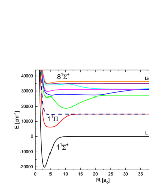
Fig.  1: Adiabatic potential energy curves of LiH: 1-8 ${}^{1}\Sigma^{+}$ states (solid lines), 1${}^{1}\Pi$ state (dashed line).

Several characteristic avoided crossings are visible, particularly the double one at 5 and 20 $a_{0}$ between the curves of the $3^{1}\Sigma$ and $4^{1}\Sigma$ states. Though not very pronounced, there are avoided crossings between $1^{1}\Sigma$ and $2^{1}\Sigma$ at 7.5 $a_{0}$ and $2^{1}\Sigma$ and $3^{1}\Sigma$ at 10 $a_{0}$.

Equilibrium positions R_e and depths of the potential wells D_e are compared with other theoretical and experimental results in Table 2.

Table 2:  Spectroscopic parameters R_e [a₀], D_e, $\omega_{e}$, and T_e [cm^-1] for the ground and low-excited states of the $\rm LiH$ molecule

State	Dissociation limit	Author	Re	De	$\omega_{e}$	Te
$1^{1}\Sigma^{+}$	Li(2s) + H(1s)	present (theory)	3.003	20327	1391
		Aymar 2009 (theory) 21	3.002	20167	1398
		Gadea 2006 (theory) 2	3.003	20349
		Dolg 1996 (theory) 49	3.000	20123	1391
		Stwalley 1993 (exp.) 1	3.015	20288	1407
		Boutalib 1992 (theory) 6	3.007	20174
$2^{1}\Sigma^{+}$	Li(2p) + H(1s)	present (theory)	4.866	8687	260	26544
		Aymar 2009 (theory) 21	4.820	8698	241
		Gadea 2006 (theory) 2	4.862	8687
		Stwalley 1993 (exp.) 1	4.906	8679
		Boutalib 1992 (theory) 6	4.847	8690		26390
		Vidal 1982 (theory) 53	4.910	8686	244
$1^{1}\Pi$		present (theory)	4.50	286	226	34945
		Velasco 1957 (exp.) 33	4.49	284	216
		Vidal 1982 (theory) 53	4.50	289
		Aymar 2009 (theory) 21	4.52	251	243
$3^{1}\Sigma^{+}$	Li(3s)+H(1s)	present (theory)	3.821	1270	540	46259
			10.172	8438	293	39092
		Aymar 2009 (theory) 21	3.830	1267	390
			10.150	8361	390
		Gadea 2006 (theory) 2	3.821	-
			10.181	8453
		Huang 2000 (exp.) 50	-	-
			10.140	8469
		Boutalib 1992 (theory) 6	3.825	1277		46109
			10.206	8444		38942

For the ground state our position of $R_{e}$ agrees exactly with the theoretical value of Dolg ⁴⁹ and reasonably with the experimental value of Stwalley et al. ¹. We also find a good agreement within 40 cm^-1 between the well depths $D_{e}$ of our results and experimental data of Stwalley et al. In the case of 1${}^{1}\Pi$, our results of R_e and D_e agree within 2 cm^-1 with the experimental data of Velasco. All theoretical results indicate the existence of a double well for the $3^{1}\Sigma$ state but this is not confirmed by the only available experiment by Huang et al. ⁵⁰.

FIG. 2 displays spacings between successive rovibrational levels of the $1^{1}\Pi$ state. Our first set of values is obtained by solving ⁵¹ Eq. 8. The second one comes from appropriate differences between the positions of peaks in the absorption spectrum obtained from Eq. 16 and presented in FIG. 3. These two sets agree very well with each other. Moreover, there is also very good agreement with the experimental values of Velasco ³³.

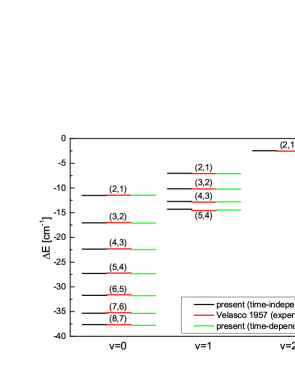
Fig.  2: Differences $\Delta E(v,J^{\prime},J)=E(v,J^{\prime})-E(v,J)$ between rovibrational levels with the same vibrational quantum number $v$ of the $1^{1}\Pi$ state. Three series of differences are drawn for $v=1,2$ and $3$. Each difference is specified by $(J,J^{\prime})$. The blue lines are coming from calculated rovibrational levels. The red ones are derived from experimental data of Velasco ³³. The green ones are our results obtained from the absorption spectrum shown in FIG. 3.

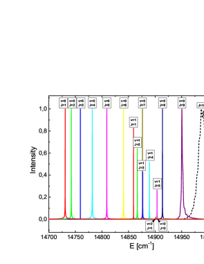
Fig.  3: The total absorption cross section calculated from Eq. 16.

The peaks in the absorption spectrum (FIG. 3) are obtained by solving the time dependent Schrödinger equation⁵² (Eq. 12) with a Gaussian-shaped wavepacket $\Phi$ initially centered at 6.15 $a_{0}$ and possessing the half-width equal to $0.95\ a_{0}$. Here, we are not interested in the intensity of the peaks and the precise shape of the initial wave packet is unimportant. The set of effective potentials $U_{J}$ (Eq. 7) spans $J$ from $1$ to $10$. The broadened peak labeled by $v=0$ and $J=9$ is the last in the series since $J=9$ is a critical value $J_{c}$ discussed in Section 2.2. Its half-width (FWHM) is equal to 2.7 cm^-1. The last very broad peak with $J=10$ illustrates the situation where the depth of the effective potential is too shallow to allow for existence of any bound vibrational level. The last and already broadened peak observed by Velasco was assigned as $v=0$ and $J=8$. In his analysis, he correctly foreseen the existence of an unobserved peak labeled by $v=0$ and $J=9$ before the molecule breaks off due to high rotations. But his prediction of existence of two other missing peaks in the spectrum, namely with $v=1$, $J=6$ and $v=2$, $J=3$ is not confirmed by our results. The broadening of the peak with $v=0$ and $J=9$ showed by our calculation is due to quantum tunneling through the centrifugal barrier.

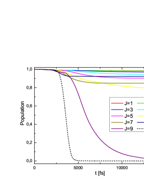
Fig.  4: Time-dependent population of the wavepacket placed on the effective potential $U_{J}(R)$ (J=1,…,10) for electronic energy of the $1^{1}\Pi$ state. All lines refer to the same initial conditions at $t=0$ of the wavepacket.

The last figure (FIG. 4) shows the results for the time dependent population of the 1${}^{1}\Pi$ state for the same initial condition. For $J=10$, no bound states are supported by the effective potential and the drop in population around 2.5 ps shows the time it takes for the continuum wave packet to reach $R=R_{max}$. In our calculations, we set this value to be equal to 100 $a_{0}$. In all cases, the population is close to one within the first approximately 2.5 ps, since any continuum part of the wave packet needs this time to reach $R_{max}$. Furthermore for low values of $J$, the population is close to one within the time window of 15 ps, meaning that essentially all parts of the wave packet can be represented by bound states. For $J=9$, the wave packet consists of a continuum as well as a (quasi-) bound part. The quasibound part decays via tunneling giving rise to the slow exponential decay with a decay constant of 2.4 ps. Based on the time-energy uncertainty principle, we can estimate that this lifetime should give rise to a line width of approximately 2 cm^-1. This is in good agreement with the spectrum in FIG. 3.

4 Conclusions

In order to describe the rotational predissociation process of the LiH molecule we start from calculating the low lying adiabatic potential energy curves with particular emphasis on the $1^{1}\Pi$ state. Our spectroscopic parameters are in very good agreement with experimental values. Having the potential curve of $1^{1}\Pi$ state we calculate the rovibrational levels. The differences between these successive levels are compared with those derived from experimental data of Velasco. The agreement again is very good, which means that the shape of the first excited electronic state $1^{1}\Pi$ is reliable. On the other hand since our difference ($T_{e}$) between potential wells of $1^{1}\Pi$ and of the ground state $1^{1}\Sigma^{+}$ is around 50 cm^-1 larger than experimental value of Stwalley et al., the direct comparison with the spectrum of Velasco shows a small systematic shift.

In order to get insights from the complementary time-dependent approach we solve the time-dependent nuclear Schrödinger equation. The solution shows the evolving wavepacket originally placed on the effective potential curve. The absorption spectrum is calculated as a Fourier transform of the autocorrelation function. The differences between successive peaks in the spectrum are compared with those of Velasco and ours obtained in the time-independent approach. All three sets of values are in very good agreement. Our results for time-dependent population of the $1^{1}\Pi$ state explain in detail the rotational predissociation mechanism of the LiH molecule. A challenge for experimentalist would be to detect in real time (via pump-probe spectroscopy) the predissociation due to quantum tunneling through the centrifugal barrier.

References

- 1 W.C. Stwalley, W.T. Zemke, J. Phys. Chem. Ref. Data 22, 87 (1993).
- 2 F.X. Gadea, T. Leininger, Theor. Chem. Acc. 116, 566 (2006).
- 3 F.H. Crawford, T. Jorgensen Jr., Phys. Rev. 47, 932 (1935).
- 4 F.H. Crawford, T. Jorgensen Jr., Phys. Rev. 49, 745 (1936).
- 5 N.L. Singh, D.C. Jain, Proc. Phys. Soc. 79, 753 (1962).
- 6 A. Boutalib, F.X. Gadea, J. Chem. Phys. 97, 1144 (1992).
- 7 M.E. Casida, F. Gutierrez, J. Guan, F.X. Gadea, D. Salahub, J.P. Daudey, J. Chem Phys. 113, 7062 (2000).
- 8 H. Beriche, F.X. Gadea, Eur. Phys. J. D 70, 2 (2016).
- 9 F.X. Gadea, A. Boutalib, J. Phys. B: At. Mol. Opt. Phys. 26, 61 (1993).
- 10 F. Gemperle, F.X. Gadea, Europhys. Lett. 48, 513 (1999).
- 11 A.S. Dickinson, F.X. Gadea, Mon. Not. R. Astron. Soc. 318, 1227 (2000).
- 12 B.O. Roos, A.J. Sadlej, J. Chem. Phys. 76, 5444 (1982).
- 13 A.K. Sharma, S. Chandra, J. Phys. B: At. Mol. Opt. Phys. 33, 2623 (2000).
- 14 F.A. Gianturco, P. Gori Giorgi, Phys. Rev. A 54, 4073 (1996).
- 15 F.A. Gianturco, P. Gori Giorgi, H. Berriche, F.X. Gadea, Astron. Astrophys. Suppl. Series 117, 377 (1996).
- 16 S. Bubin, L. Adamowicz, J. Chem. Phys. 121, 6249 (2004).
- 17 P.C. Stancil, A. Dalgarno, Astrophys. J. 479, 543 (1997).
- 18 E. Bodo, F.A. Gianturco, R. Martinazzo, Phys. Rep.-Rev. Sect. Phys. Lett. 384, 85 (2003).
- 19 R. Fondermann, M. Hanrath, M. Dolg, Theor. Chem. Account 118, 777 (2007).
- 20 J.R. Trail, R.J. Needs, J. Chem. Phys. 128, 204103 (2008).
- 21 M. Aymar, J. Deiglmayr, O. Dulieu, Can. J. Phys. 87 543 (2009).
- 22 I.L. Cooper, A.S. Dickinson, J. Chem. Phys. 131, 204303 (2009).
- 23 R. Côté, E. Juarros, K. Kirby, Phys. Rev. A 81, 060704 (2010).
- 24 M. Cafiero, L. Adamowicz, Phys. Rev. Lett. 88, 033002 (2002).
- 25 F. M. Fernandez, J. Chem. Phys. 130, 166101 (2009).
- 26 P. Decleva, A. Lisini, J. Phys B 19, 981 (1986).
- 27 S. Magnier, J. Phys. Chem. 108, 1052 (2004).
- 28 M. Cheng, J. M. Brown, P. Rosmus, R. Linguerri, N. Komiha, E. G. Myers, Phys. Rev. A 75, 012502, (2007).
- 29 W.-C. Tung, M. Pavanello, L. Adamowicz, J. Chem. Phys. 134, 064117 (2011).
- 30 F. Holka, P. G. Szalay, J. Fremont, M. Rey, K. A. Peterson, V. G. Tyuterev, J. Chem. Phys. 134, 094306 (2011).
- 31 R. S. Mulliken, Phys. Rev., 50,1028 (1936).
- 32 M. Nest, F. Remacle, R. D. Levine, New J. Phys. 10, 025019 (2008).
- 33 R. Velasco, Can. J. Phys. 35, 1204 (1957).
- 34 A.H. Zewail, Femtochemistry. Ultrafast dynamics of the chemical bond. Volume I and II, World Scientific Publishing Co. Pte. Ltd., Singapore 1994.
- 35 M. Grønager, N.E. Henriksen, J. Chem. Phys. 104, 3234 (1996).
- 36 M. Grønager, N.E. Henriksen, J. Chem. Phys. 109, 4335 (1998).
- 37 H. Dietz, V. Engel, J. Phys. Chem. A 102, 7406 (1998).
- 38 K.B. Møller, N.E. Henriksen, A.H. Zewail, J. Chem. Phys. 113, 10477 (2000).
- 39 K. R. Way, W. C. Stwalley, J. Chem. Phys. 59, 5298 (1973).
- 40 P. Fuentealba, H. Preuss, H Stoll, L. Von Szentply, Chem. Phys. Letters 89, 418 (1982).
- 41 E. Czuchaj, F. Rebentrost, H. Stoll and H. Preuss, Theor. Chem. Acc. 100, 117 (1998).
- 42 E. Czuchaj, M. Krośnicki and H. Stoll, Chem. Phys. 292, 101 (2003).
- 43 M. Dolg, Effective Core Potentials in Modern Methods and Algorithms of Quantum Chemistry, J. Grotendorst (Ed.), NIC Series, Vol. 3, 540 (2000).
- 44 Private communication, as cited in MOLPRO manual (http://www.molpro.net).
- 45 C. E. Moore, Atomic energy levels as derived from the analysis of optical spectra - Hydrogen through Vanadium. Vol. I, Circular of the National Bureau of Standards, 467, U. S. Government Printing Office, Washington, 1949.
- 46 MOLPRO, version 2012.1, is a package of ab initio programs written by H.-J. Werner, P. J. Knowles, G. Knizia, F. R. Manby, M. Schütz, P. Celani, W. Györffy, D. Kats, T. Korona, R. Lindh, A. Mitrushenkov, G. Rauhut, K. R. Shamasundar, T. B. Adler, R. D. Amos, A. Bernhardsson, A. Berning, D. L. Cooper, M. J. O. Deegan, A. J. Dobbyn, F. Eckert, E. Goll, C. Hampel, A. Hesselmann, G. Hetzer, T. Hrenar, G. Jansen, C. Köppl, Y. Liu, A. W. Lloyd, R. A. Mata, A. J. May, S. J. McNicholas, W. Meyer, M. E. Mura, A. Nicklaß, D. P. O’Neill, P. Palmieri, D. Peng, K. Pflüger, R. Pitzer, M. Reiher, T. Shiozaki, H. Stoll, A. J. Stone, R. Tarroni, T. Thorsteinsson, M. Wang, see http://www.molpro.net.
- 47 D.J. Tannor, Introduction to quantum mechanics: a time-dependent perspective, University Science Books, Sausalito, 2007.
- 48 L.D. Landau, E. Lifshitz, Quantum Mechanics, Pergamon, New-York, 1965.
- 49 M. Dolg, Theo. Chem. Acc. 93, 141 (1996).
- 50 Y.L. Huang, W.T. Luh, G.H. Jeung, F.X. Gadea, J. Chem. Phys. 113, 683 (2000).
- 51 R.J. Le Roy, LEVEL: A computer program for solving the radial Schrödinger equation for bound and quasibound levels, J. Quant. Spectrosc. Radiat. Transfer 186, 167 (2017).
- 52 B. Schmidt and U. Lorenz, WavePacket: A Matlab package for numerical quantum dynamics. I: Closed quantum systems and discrete variable representations, Comp. Phys. Comm. 213, 223 (2017); B. Schmidt and C. Hartmann, WavePacket: A Matlab package for numerical quantum dynamics. II: Open quantum systems and optimal control, manuscript in preparation (2017).
- 53 C.R. Vidal, W.C. Stwalley, J. Chem. Phys. 77, 883 (1982).