Time-triggering versus event-triggering control over communication channels

Abstract

Time-triggered and event-triggered control strategies for stabilization of an unstable plant over a rate-limited communication channel subject to unknown, bounded delay are studied and compared. Event triggering carries implicit information, revealing the state of the plant. However, the delay in the communication channel causes information loss, as it makes the state information out of date. There is a critical delay value, when the loss of information due to the communication delay perfectly compensates the implicit information carried by the triggering events. This occurs when the maximum delay equals the inverse of the entropy rate of the plant. In this context, extensions of our previous results for event triggering strategies are presented for vector systems and are compared with the data-rate theorem for time-triggered control, that is extended here to a setting with unknown delay.

I Introduction

Internet of things establishes a foundation for emerging of engineering systems that integrate computing, communication, and control, these systems are know as cyber-physical systems (CPS) [1, 2]. One key aspect of CPS is the presence of finite-rate, digital communication channels in the feedback loop. To quantify their effect on the ability to stabilize the system, data-rate theorems have been developed [3, 4]. They essentially state that, in order to achieve stabilization, the communication rate available in the feedback loop should be at least as large as the entropy rate of the system, corresponding to the sum of the logarithms of the unstable modes. In this way, the controller can compensate for the expansion of the state occurring during communication

More recent formulations of data-rate theorems include stochastic, time-varying, Markovian, erasure, additive white and colored Gaussian, and multiplicative noise feedback communication channels [5, 6, 7, 8, 9, 10], formulations for nonlinear sytems [11, 12, 13], and for systems with uncertain and variable parameters [14, 15, 16, 17]. Connections with information theory are highlighted in [13, 18, 19, 20, 21]. Extended surveys of the literature appear in [22] and [23].

Another important aspect of CPS is the need to use distributed resources efficiently. In this context, event-triggering control techniques [24, 25] have emerged. These are based on the idea of sending information in an opportunistic manner between the controller and the plant. In this way, communication occurs only when needed, and the primary focus is on minimizing the number of transmissions while guaranteeing the control objectives. Some recent results on event-triggered implementations in the presence of data rate constraints appear in [26, 27, 28, 29]. One important observation raised in [27] is that using event-triggering is possible to “beat” the data-rate theorem. More precisely, if the channel does not introduce any delay, then an event-triggering strategy can achieve stabilization for any positive rate of transmission. This apparent contradiction is resolved by realizing that the timing of the triggering events carries information, revealing the state of the system. When communication occurs without delay, the state can be tracked with arbitrary precision, and transmitting a single bit at every triggering event is enough to compute the appropriate control action.

In our previous work [30], we extended the above observation to the whole spectrum of possible delay values. Key to our analysis was the distinction between the information access rate, that is the rate at which the controller needs to receive data, regulated by the classic data-rate theorem; and the information transmission rate, that is the rate at which the sensor needs to send data, regulated by a given triggering control strategy. For a given triggering strategy, we showed that for sufficiently low values of the delay, the timing information carried by the triggering events is large enough and the system can be stabilized with any positive information transmission rate. At a critical value of the delay, the timing information carried by event triggering is not enough for stabilization and the required information transmission rate begins to grow. When the delay reaches the inverse of the entropy rate of the plant, the timing information becomes completely obsolete, and the required information transmission rate becomes larger than the information access rate imposed by the data-rate theorem.

In the present work, we compare these results with those of a time-triggered implementation, for which we provide a formulation of the data-rate theorem for continuous-time systems in the presence of delay. The comparison leads to additional insights on the value of information in event triggering. We also extend results in [30] to vector systems. Proofs of the results on event-triggering are omitted and can be found in [31].

Notation

Let $\mathbb{R}$ and $\mathbb{N}$ denote the set of real and positive integer numbers, respectively. We denote by $\mathcal{B}(\epsilon)$ the ball centered at $0$ of radius $\epsilon$. We let $\log$ and $\ln$ denote the logarithm with bases $2$ and $e$, respectively. For any function $f:\mathbb{R}\rightarrow\mathbb{R}^{n}$ and $t\in\mathbb{R}$, we let $f(t^{+})$ denote the limit from the right, namely $\lim_{s\downarrow t}f(s)$. We let $M_{n,m}(\mathbb{R})$ be the set of $n\times m$ matrices over the field of real numbers. Let $0_{n}$ be the all $0$ vector of size $n$. Given $A=[a_{i,j}]_{1\leq i,j\leq n}\in M_{n,n}(\mathbb{R})$, we let $\operatorname*{tr}(A)=\sum_{i=1}^{n}a_{ii}$ and $\det(A)$ denote its trace and determinant, respectively. Note that $\det(e^{A})$ is equal to $e^{\operatorname*{tr}(A)}$. We let $m$ denote the Lebesgue measure on $\mathbb{\mathbb{R}}^{n}$, which for $n=2$, and $n=3$ corresponds to area and volume, respectively. Note that for $A\in M_{n,n}(\mathbb{R})$ and $X\in\mathbb{R}^{n}$, $m(AX)=|\det(A)|m(X)$. We let $\lfloor x\rfloor$ denote the greatest integer less than or equal to $x$. We let $\|x\|$ be the $L^{2}$ norm of $x$ in $\mathbb{R}^{n}$.

II Problem formulation

System model

We consider a networked control system composed by the plant-sensor-channel-controller tuple depicted in Figure 1.

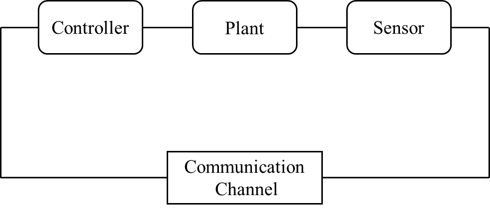
Figure 1: System model.

The plant dynamics are described by a vector, continuous-time, linear time-invariant (LTI) system

$$\dot{x}=Ax(t)+Bu(t),$$ (1)

where $x(t)\in\mathbb{R}^{n}$ and $u(t)\in\mathbb{R}^{m}$ for $t\in[0,\infty)$ are the plant state and control input, respectively. Here, $A\in M_{n,n}(\mathbb{R})$, $B\in M_{n,m}(\mathbb{R})$, and

$$x(0)\in\mathcal{B}(L)$$

for some non-negative real number $L$ ($L$ is known to both sensor and controller). Without loss of generality, we assume that all the eigenvalues of $A$ are unstable, that is, $\text{Re}\{\lambda_{i}\}>0$ for $i\in\{1,\ldots,n\}$. The sensor can measure the state of the system exactly, and the controller can apply the control input to the plant with infinite precision and without delay. However, sensor and controller communicate through a channel that can support only a finite data rate and is subject to delay, as we describe next.

Triggering Times and Communication Delay

We denote by $\{t_{s}^{k}\}_{k\in\mathbb{N}}$ the sequence of times at which the sensor transmits a packet composed of $g(t_{s}^{k})$ bits representing the system state to the controller. We define the $k^{th}$ triggering interval by

$$\Delta^{\prime}_{k}=t_{s}^{k+1}-t_{s}^{k}.$$ (2)

We let $t_{c}^{k}$ be the time at which the controller receives and decodes a packet of data which was encoded and transmitted at time $t_{s}^{k}$ for $k\in\mathbb{N}$. We assume a uniform upper bound, known to the sensor and the controller, on the communication delays

$$\Delta_{k}=t_{c}^{k}-t_{s}^{k}\leq\gamma.$$ (3)

When referring to a generic triggering time or reception time, we shall skip the superscript $k$ in $t_{s}^{k}$ and $t_{c}^{k}$.

Time-Triggered and Event-Triggered Control

With the information received from the sensor, the controller maintains an estimate $\hat{x}$ of the plant state, which during the inter-reception times evolves according to

$$\dot{\hat{x}}(t)=A\hat{x}(t)+Bu(t),$$ (4)

starting from $\hat{x}(t_{c}^{k+})$.

The state estimation error is then

$$z(t)=x(t)-\hat{x}(t),$$ (5)

where $z(0)=x(0)-\hat{x}(0)$. Without updated information from the sensor, this error grows, and the system can potentially become unstable. The sensor should therefore select the sequence of transmission times $\{t_{s}^{k}\}_{k\in\mathbb{N}}$ and the packet sizes $\{g(t^{k}_{s})\}_{k\in\mathbb{N}}$ in a way that ensures stabilizability and observability, while satisfying the rate constraints imposed by the channel.

The asymptotic notions of stabilizability and observability that we require are standard, and are formally defined in [3, 30]. To ensure these asymptotic properties, we consider two different approaches: event-triggered and time-triggered control. In an event-triggering implementation, we define a triggering function $v(t)$ that is known to both the controller and the sensor. Whenever the state estimation error crosses the value of this function, a transmission occurs. In a time-triggered implementation, transmissions are not state dependent.

Information Access Rate

We let $b_{c}(t)$ denote the number of bits that have been received by the controller up to time $t$. We define the information access rate

$$R_{c}=\limsup_{t\rightarrow\infty}\frac{b_{c}(t)}{t}.$$ (6)

In this setting, data-rate theorems describe the trade-off between the information access rate and the ability to stabilize the system. They are generally stated for discrete-time systems, albeit similar arguments hold in continuous time as well, see e.g. [32]. They are based on the fundamental observation that there is an inherent entropy rate

$$h(A)=\frac{\operatorname*{tr}(A)}{\ln 2}=\frac{\sum_{i=1}^{d}\lambda_{i}}{\ln 2}$$ (7)

at which the plant generates information. It follows that to guarantee stability it is necessary for the controller to have access to state information at a rate

$$R_{c}>h(A).$$ (8)

This result indicates what is required by the controller, and it does not depend on the feedback structure — including aspects such as communication delays, information pattern at the sensor and the controller, and whether the times at which transmissions occur are state dependent, as in event-triggered control, or not, as in time-triggered control.

Information Transmission Rate

We now take the viewpoint of the sensor when examining the amount of information that it needs to transmit to the controller. We make the following two observations. First, in the presence of communication delays, the state estimate received by the controller might be out of date, so that the sensor might need to send data at a higher rate than what (8) prescribes to make-up for such discrepancy. Second, in the case of event-triggered transmissions, the timing of the triggering events itself carries some information. For instance, if the communication channel does not introduce any delay, then a triggering event may reveal the state of the system very precisely, and effectively carry an unbounded amount of information. The controller may then be able to stabilize the system even if the sensor uses the channel very sparingly, transmitting at a smaller rate than what (8) prescribes.

Motivated by these observations, let $b_{s}(t)$ be the number of bits transmitted by the sensor up to time $t$, and define the information transmission rate by

$$R_{s}=\limsup_{t\rightarrow\infty}\frac{b_{s}(t)}{t}.$$ (9)

Since at every triggering time the sensor sends $g(t_{s}^{k})$ bits, we also have

$$R_{s}=\limsup_{N\rightarrow\infty}\frac{\sum_{k=1}^{N}g(t_{s}^{k})}{\sum_{k=1}^{N}\Delta^{\prime}_{k}}.$$ (10)

III Necessary condition on the access rate for event triggering

We now quantify the amount of information that the controller needs to have access to in order to have exponential convergence of the estimation error and the plant state to zero, irrespective of the feedback structure used by the sensor to decide when to transmit. The proof follows, with minor modifications to the one for the scalar case, cf. [31].

Theorem 1

Consider the plant-sensor-channel-controller model described in Section II with plant dynamics (1), and state estimation error $z(t)$. Let $\sigma\in\mathbb{R}$ be positive.

1. If the state estimation error satisfies

   $$\|z(t)\|\leq\|z(0)\|~{}e^{-\sigma t},$$

   then

   $$b_{c}(t)\geq t~{}\frac{\operatorname*{tr}(A)+n\sigma}{\ln 2}+n~{}\log\frac{L}{\|z(0)\|}.$$ (11)

2. If the system is stabilizable and

   $$\|x(t)\|\leq\|x(0)\|~{}e^{-\sigma t},$$

   then

   $$b_{c}(t)\geq t~{}\frac{\operatorname*{tr}(A)+n\sigma}{\ln 2}.$$ (12)

In both cases, the information access rate is

$$R_{c}>\frac{\operatorname*{tr}(A)+n\sigma}{\ln 2}.$$ (13)

Proof:

Note that (13) immediately follows by dividing (11) and (2) by $t$ and taking the limit for $t\rightarrow\infty$. Regarding (i), let us write the solution to (1) as

$$x(t)=e^{At}x(0)+\alpha(t),\quad\alpha(t)=e^{At}\int_{0}^{t}{e^{-A\tau}Bu(\tau)d\tau}.$$ (14)

We then define,

$$\Gamma_{t}=\{x(t):x(t)=e^{At}x(0)+\alpha(t)~{};~{}\|x(0)\|\leq L\},$$ (15)

that is a set which represents the uncertainty at time $t$ given the bound $L$ on the norm of the initial condition $x(0)$ and $\alpha(t)$. The state of the system can be any point in this uncertainty set. We can find a lower bound on $b_{c}(t)$ by counting the number of balls of radius $\epsilon(t)$, that cover $\Gamma_{t}$, where $\epsilon(t)=\|z(0)\|~{}e^{-\sigma t}$. The Lebesgue measure of a sphere of radius $\epsilon$ in $\mathbb{R}^{n}$ is $k_{n}\epsilon^{n}$ where $k_{n}$ is a constant that changes with dimension. Therefore $b_{c}(t)$, the number of bits of information that the controller must have access to by time $t$, should satisfy

$$b_{c}(t) \geq\log\frac{m(\Gamma_{t})}{m(\mathcal{B}(\epsilon(t)))}$$

$$=\log\frac{|\det((e^{A})^{t})|m(\|x(0)\|\leq L)}{k_{d}\|z(0)\|^{n}~{}e^{-n\sigma t}}$$

$$=t~{}\log|\det(e^{A})e^{n\sigma}|+\log\frac{L^{n}}{\|z(0)\|^{n}}$$

$$=t~{}\log|e^{\operatorname*{tr}(A)+n\sigma}|+n\log\frac{L}{\|z(0)\|}.$$

With access to $b_{c}(t)$ bits of information, the controller can at best identify $x(t)$ up to a ball of radius $\epsilon(t)$. Consequently, (i) follows.

Recall that $\|x(0)\|\leq L$. For any given control trajectory $\{u(\tau)\}_{\tau=0}^{\tau=t}$ define

$$\Pi_{\{u(\tau)\}_{\tau=0}^{\tau=t}}=\{x(0):\|x(t)\|<\epsilon(t)\},$$

where $\epsilon(t)=\|x(0)\|~{}e^{-\sigma t}$. These are the sets of all initial conditions for which by choosing the control trajectory $\{u(\tau)\}_{\tau=0}^{\tau=t}$, the plant state at time $t$, $x(t)$, will be in a ball of radius $\epsilon(t)$. $x(t)$ depends linearly on $\{u(\tau)\}_{\tau=0}^{\tau=t}$. As a consequence, all of the sets $\Pi_{\{u(\tau)\}_{\tau=0}^{\tau=t}}$, are linear transformation of each other. The measure of $\Pi_{\{u(\tau)=0\}_{\tau\in[0,t]}}$ is

$$|\det(e^{-At})k_{n}\|x(0)\|^{n}e^{-n\sigma t}|=k_{n}\|x(0)\|^{n}e^{-(\operatorname*{tr}(A)+n\sigma)t},$$

which is upper bounded by $k_{n}L^{n}e^{-(\operatorname*{tr}(A)+n\sigma)t}$. We can then determine a lower bound for $b_{c}(t)$ by counting the number of $\Pi$ sets (for different control trajectories $\{u(\tau)\}_{\tau=0}^{\tau=t}$) which takes to cover the ball $\|x(0)\|\leq L$.

Thus, the controller must have access to at least $b_{c}(t)$ bits by time $t$, where

$$b_{c}(t) \geq\log\frac{m(\|x(0)\|\leq L)}{m(\Pi)}$$

$$=\log\frac{k_{n}L^{n}}{k_{n}\|x(0)\|^{n}e^{-(\operatorname*{tr}(A)+n\sigma)t}}$$

$$\geq t~{}\frac{\operatorname*{tr}(A)+n\sigma}{\ln 2}+n~{}\log\frac{L}{L},$$

and this proves (ii). ∎

Remark 1

Theorem 1 is valid for any control scheme, and the controller does not necessarily have to compute the state estimate following (4). This theorem can be viewed as an extension of the data-rate theorem with exponential convergence guarantees. It states that, to have exponential convergence of the estimation error and the state, the access rate should be larger than the estimation entropy, the latter concept having been recently introduced in [33]. A similar result for continuous-time systems appears in [26], but only for linear feedback controllers. The classic formula of the data-rate theorem (8), given in [3, 4] can be derived as a special case of Theorem 1 by taking $\sigma\rightarrow 0$ and using continuity. $\bullet$

IV Necessary condition on the transmission rate for time triggering

We now derive a data-rate theorem for the information transmission rate in two different time-triggered scenarios and in the presence of unknown communication delays.

In the first scenario, we assume the following time-triggered implementation: the sensor transmits at all times $\{t_{s}^{k}\}_{k\in\mathbb{N}}$, where

$$t_{s}^{k}=kT,$$ (16)

and $T$ denotes the transmission period. Note that in this setting, the sensor transmits without considering whether the previous packets have been received and decoded or not. Consequently, the communication delay is upper bounded as (3) only when there is not another packet in the communication channel. In this setting, we have the following theorem.

Theorem 2

Consider the plant-sensor-channel-controller model described in Section II with plant dynamics (1). Assume that the communication delays upper bounded as (3) when there is no other packet in the channel, and assuming that the packets are received and decoded by the controller in the order they are transmitted by the sensor. Then, there exists a delay realization $\{\Delta_{k}\}_{k\in\mathbb{N}}$ such that a rate

$$R_{s}>\left\{\begin{array}[]{ll}\dfrac{\operatorname*{tr}(A)}{\ln 2}&\mbox{ if }\gamma<T,\\ \\ \dfrac{\operatorname*{tr}(A)\frac{\gamma}{T}}{\ln 2}&\mbox{ if }\gamma\geq T.\\ \end{array}\right.$$

is necessary for asymptotic observability and asymptotic stabilizability.

Proof:

Consider an observer that can receive the packets transmitted by the sensor without any delay, and that has the same knowledge about the system as the controller. Let $\zeta_{t}^{o}$ and $\zeta_{t}^{c}$ be the uncertainty sets for the state $x(t)$, at the observer and controller, respectively. We have $\zeta_{0}^{o}=\zeta_{0}^{c}$.

We write the solution to (1) as (14). Consequently, we have

$$m(\zeta_{t_{s}^{(k+1)-}}^{o})=e^{\operatorname*{tr}(A)T}m(\zeta_{t_{s}^{k}}^{o}).$$

Since the observer receives packets without delay, we have

$$m(\zeta_{t_{s}^{k+1}}^{o})\geq\frac{1}{2^{g(t_{s}^{k})}}m(\zeta_{t_{s}^{(k+1)-}}^{o})=\frac{1}{2^{g(t_{s}^{k})}}e^{\operatorname*{tr}(A)T}m(\zeta_{t_{s}^{k}}^{o}).$$

By iterating from $k=1$ to $k=\eta$, we have

$$m(\zeta_{t_{s}^{\eta-}}^{o})\geq\dfrac{1}{2^{\sum_{k=1}^{k=\eta-1}g(t_{s}^{k})}}e^{\operatorname*{tr}(A)\eta T}m(\zeta_{0}^{o}).$$

However, the controller does not necessarily receive packets immediately. Indeed, in the worst case, if $\gamma>T$ the controller receives packets that have been sent in the time interval $[0,\eta T)$ by the time $\eta T+\eta(\gamma-T)=\eta\gamma$. While, for $T>\gamma$ we have

$$m(\zeta_{t_{c}^{\eta-}}^{c})\geq m(\zeta_{t_{s}^{\eta-}}^{o}),$$ (17)

for $T\leq\gamma$ we have

$$\sup_{\{\Delta_{k}\}\leq\gamma}m(\zeta_{t_{c}^{\eta-}}^{c})\geq m(\zeta_{t_{s}^{\eta-}}^{o})e^{\operatorname*{tr}(A)\eta(\gamma-T)}.$$ (18)

It follows that the right-hand side of (17) and (18) tends to infinity as $\eta\rightarrow\infty$, making it impossible to stabilize or track the state, if

$$\infty =\lim_{\eta\rightarrow\infty}\dfrac{1}{2^{\sum_{k=1}^{k=\eta-1}g(t_{s}^{k})}}e^{\operatorname*{tr}(A)\eta T}$$

$$=\lim_{\eta\rightarrow\infty}\exp\left\{T\eta\left(\operatorname*{tr}(A)-\ln 2\frac{\sum_{k=1}^{k=\eta-1}g(t_{s}^{k})}{T\eta}\right)\right\}$$

for $T>\gamma$, and

$$\infty =\lim_{\eta\rightarrow\infty}\dfrac{1}{2^{\sum_{k=1}^{k=\eta-1}g(t_{s}^{k})}}e^{\operatorname*{tr}(A)\eta\gamma}$$

$$=\lim_{\eta\rightarrow\infty}\exp\left\{T\eta\left(\operatorname*{tr}(A)\frac{\gamma}{T}-\ln 2\frac{\sum_{k=1}^{k=\eta-1}g(t_{s}^{k})}{T\eta}\right)\right\}$$

for $T<\gamma$. The result now follows. ∎

Remark 2

Theorem 2 provides a data-rate theorem for the information transmission rate without imposing exponential convergence guarantees. It shows the existence of a critical delay value $\gamma=T$, at which the rate begins to increase linearly with the delay. $\bullet$

We next consider a different time-triggered scenario. Let

$$t_{s}^{0}=0,\quad t_{s}^{k+1}=t_{s}^{k}+(\lfloor\Delta_{k}/T\rfloor+1)T,$$ (19)

where $T$ is a fixed non-negative real number. In this case, the sensor transmits only at integer multiples of the period $T$, after the previous packet is received. It follows that there is no delay accumulation, and for all packets the delay satisfies (3). In this setting, we have the following result for exponential convergence of the estimation error to zero.

Theorem 3

Consider the plant-sensor-channel-controller model described in Section II with plant dynamics (1), and state estimation error $z(t)$. Let $\sigma\in\mathbb{R}$ be positive. If using the time-triggered implementation (19) the state estimation error satisfies

$$\|z(t_{s}^{k})\|\leq\|z(0)\|~{}e^{-\sigma t_{s}^{k}},$$ (20)

for all $k\in\mathbb{N}$, then there exists a delay realization $\{\Delta_{k}\}_{k\in\mathbb{N}}$ which requires

$$R_{s}\geq\frac{(\operatorname*{tr}(A)+n\sigma)(\lfloor\frac{\gamma}{T}\rfloor+1)}{\ln 2}.$$ (21)

Proof:

Using (14) we know the state of the system can be any point in $\Gamma_{t}$, cf. (15), then, we have

$$m(\Gamma_{t_{c}^{k}})=e^{\operatorname*{tr}(A)\Delta_{k}}m(\Gamma_{t_{s}^{k}}),$$

and

$$m(\Gamma_{t_{s}^{k+1}})\geq m(\Gamma_{t_{c}^{k}})e^{\operatorname*{tr}(A)\left((\lfloor\frac{\Delta_{k}}{T}\rfloor+1)T-\Delta_{k}\right)}.$$

Iterating from $k=0$ to $k=\eta$, we have

$$m(\Gamma_{t_{s}^{\eta-}})\geq e^{\sum_{k=0}^{k=\eta-1}\operatorname*{tr}(A)(\lfloor\frac{\Delta_{k}}{T}\rfloor+1)T}m(\Gamma_{0})=e^{\operatorname*{tr}(A)t_{s}^{\eta}}m(\Gamma_{0}).$$

We can now obtain a lower bound on $\sum_{k=0}^{k=\eta-1}g(t_{s}^{k})$ by counting the number of balls of radius $\|z(0)\|~{}e^{-\sigma t_{s}^{\eta}}$, that cover $\Gamma_{t_{s}^{\eta-}}$. Recall that the Lebesgue measure of a sphere of radius $r$ in $\mathbb{R}^{n}$ is $k_{n}r^{n}$ where $k_{n}$ is a constant that depends on the dimension. We have

$$\sum_{k=0}^{k=\eta-1}g(t_{s}^{k}) \geq\log\frac{e^{\operatorname*{tr}(A)t_{s}^{\eta}}m(\Gamma_{0})}{k_{n}\|z(0)\|^{n}~{}e^{-n\sigma t_{s}^{\eta}}}$$

$$=\log\frac{e^{(\operatorname*{tr}(A)+n\sigma)t_{s}^{\eta}}m(\Gamma_{0})}{k_{n}\|z(0)\|^{n}}.$$

Hence,

$$\sum_{k=0}^{k=\eta-1}g(t_{s}^{k})\geq\log\frac{e^{(\operatorname*{tr}(A)+n\sigma)\eta(\lfloor\frac{\gamma}{T}\rfloor+1)T}m(\Gamma_{0})}{k_{n}\|z(0)\|^{n}},$$

because the sensor, not having any fore-knowledge of the delay, must send at least the number of bits required when $\Delta_{k}=\gamma$ for all $k\in\mathbb{N}$, to ensure that (20) holds. However, the actual realization of the delay may be $\Delta_{k}=0$ for all $k\in\mathbb{N}$, so that we have

$$R_{s}\geq\lim_{\eta\rightarrow\infty}\frac{1}{\eta T}\log\dfrac{e^{(\operatorname*{tr}(A)+n\sigma)\eta(\lfloor\frac{\gamma}{T}\rfloor+1)T}m(\Gamma_{0})}{k_{n}\|z(0)\|^{n}},$$

and the result follows. ∎

Remark 3

In the time-triggered setting governed by (16), a packet is transmitted without considering whether the previous packets have been received and decoded. On the other hand, in the time-triggered setting governed by (19) a packet is transmitted only after the previous packet is received. Letting $\sigma\rightarrow 0$, for $\gamma<T$ both Theorems 2 and 3 reduce to $R_{s}\geq\operatorname*{tr}(A)/\ln 2$. Namely, for low values of the delay, and without imposing exponential convergence guarantees, we recover the critical value of the data-rate theorem for the access rate in Theorem 1. $\bullet$

Remark 4

Theorem 2 and 3 are valid for any control scheme, and the controller does not necessarily have to compute the state estimate as (4). These theorems can be seen as an extension of the data-rate theorem for the information transmission rate for time-triggered control, with unknown bounded delay. $\bullet$

V Necessary and sufficient conditions on the transmission rate for event-triggering

V-A Component-wise description

In the proposed event-triggered design, we deal with each coordinate of the system separately. This corresponds to treating the $n$-dimensional system as $n$ scalar, coupled systems. When a triggering occurs for one of the coordinates, the controller should be aware of which coordinate of the system the received packet corresponds to. Accordingly, we assume that there are $n$ parallel finite-rate digital communication channels between each coordinate of the system and the controller, each subject to unknown, bounded delay. In the case of a single communication channel, we can consider the same triggering strategy, but an additional $\lceil\log n\rceil$ bits should be appended at the beginning of each packet to identify the coordinate it belongs to.

For deriving our necessary and sufficient conditions for vector system, we assume that all of the eigenvalues of $A$ are real. Recall that every $A\in M_{n,n}(\mathbb{R})$ can be written as $\Phi\Psi\Phi^{-1}$, where $\Phi$ is a real-valued invertible matrix and $\Psi=\text{diag}[J_{1},\ldots,J_{q}]$, where each $J_{j}$ is a Jordan block corresponding to the real-valued eigenvalue $\lambda_{j}$ of $A$ [34]. We let $d_{j}$ indicate the order of each $J_{j}$. Without loss of generality assume $A$ is equal to its Jordan block decomposition, that is, $A=\text{diag}[J_{1},\ldots,J_{q}]$. With the notation of Section II, we let $x_{i}^{j}(t)$, $\hat{x}_{i}^{j}(t)$, and $z_{i}^{j}(t)$ be the state, state estimation, and state estimation error for the $i^{th}$ coordinate of $j^{th}$ Jordan block, respectively. For each coordinate $i$ of the $j^{th}$ Jordan block we let $\{t_{s,i}^{k,j}\}_{k\in\mathbb{N}}$, $\{t_{c,i}^{k,j}\}_{k\in\mathbb{N}}$, $g(t_{s,i}^{k,j})$ be the sequence of transmission times, reception times, and the number of bits that are transmitted at each triggering time. Similarly, the $k^{th}$ communication delay and $k^{th}$ triggering interval can be specified for each coordinate. Following (3), we have

$$\Delta_{k,i}^{j}=t_{c,i}^{k,j}-t_{s,i}^{k,j}\leq\gamma.$$ (22)

When referring to a generic triggering or reception time, we shall skip the superscript $k$ in $t_{s,i}^{k,j}$ and $t_{c,i}^{k,j}$.

An event is triggered for coordinate $i$ in Jordan block $j$ whenever

$$|z_{i}^{j}(t_{s,i}^{j})|=v_{i}^{j}(t_{s,i}^{j}),$$ (23a)

where $$v_{i}^{j}(t)$$ is the event-triggering function

$$v_{i}^{j}(t)=v_{0,i}^{j}e^{-\sigma t},$$ (23b)

where $$v_{0,i}^{j} \sigma$$ and are positive real numbers.

Let $\bar{z}_{i}^{j}(t_{c,i}^{j})$ be an estimate of ${z}_{i}^{j}(t_{c,i}^{j})$ constructed by the controller knowing $|z_{i}^{j}(t_{s,i}^{j})|=v_{i}^{j}(t_{s,i}^{j})$, the bound (22), and the decoded packet received through the communication channel. We define the following updating procedure, called jump strategy

$$\hat{x}_{i}^{j}(t_{c,i}^{j+})=\bar{z}_{i}^{j}(t_{c,i}^{j})+\hat{x}_{i}^{j}(t_{c,i}^{j}).$$ (23c)

Note that with this jump strategy, we have

$$z_{i}^{j}(t_{c,i}^{j+})=x_{i}^{j}(t_{c,i}^{j})-\hat{x}_{i}^{j}(t_{c,i}^{j+})=z_{i}^{j}(t_{c,i}^{j})-\bar{z}_{i}^{j}(t_{c,i}^{j}).$$

When a triggering occurs for coordinate $i$ of the $j^{th}$ Jordan block, we assume that the sensor sends enough bits to ensure

$$|z_{i}^{j}(t_{c,i}^{j+})|\leq\rho(t_{s,i}^{j}):=\rho_{0}e^{-\sigma\gamma}v(t_{s,i}^{j}).$$ (23d)

When referring to a generic Jordan block, we skip the superscript and subscript $j$. For the scalar case we skip the subscript $i$ too.

The transmission rate for each coordinate is then

$$R_{s,i}^{j}=\limsup_{N_{i}^{j}\rightarrow\infty}\frac{\sum_{k=1}^{N_{i}^{j}}g(t_{s,i}^{k,j})}{\sum_{k=1}^{N_{i}^{j}}\Delta^{\prime j}_{k,i}}$$

Assuming $n$ parallel communication channels between the plant and the controller, each devoted to a coordinate separately, we have

$$R_{s}=\sum_{j=1}^{q}\sum_{i=1}^{d_{j}}R_{s,i}^{j}.$$

To obtain our necessary condition, we need to restrict the class of allowed quantization policies. We assume that, at each triggering event, there exists a delay such that the sensor can reduce the estimation error at the controller to at most a fraction of the maximum value $\rho(t_{s,i}^{j})$ required by (23d). This is a natural assumption, see [31].

Assumption 1

The controller can only achieve $\nu$-precision quantization, namely there exists $\nu\geq 1$, and a delay at most $\beta:=\frac{1}{A}\ln(1+2\rho_{0}e^{-\sigma\gamma})$, such that

$$|z(t_{c,i}^{j})-\bar{z}(t_{c,i}^{j})|\geq\frac{\rho(t_{s,i}^{j})}{\nu}.$$

V-B Review of results in the scalar case

The following results for scalar systems are the building blocks for our vector case derivation and appear in [31].

Theorem 4

Consider the plant-sensor-channel-controller model described in Section II with plant dynamics (1), estimator dynamics (4), and $n=1$. If using the event-triggering strategy (23), packet sizes such that $z(t_{c})$ is determined at the controller within a ball of radius $\rho(t_{s})=\rho_{0}e^{-\sigma\gamma}v(t_{s})$ with $\nu$-precision, and the state estimation error satisfies (20), then there exists a delay realization $\{\Delta_{k}\}_{k\in\mathbb{N}}$ which requires

$$R_{s}\geq\frac{A+\sigma}{\ln\nu+\ln(2+\frac{e^{\sigma\gamma}}{\rho_{0}})}\max\left\{0,\log\frac{(e^{A\gamma}-1)}{\rho_{0}e^{-\sigma\gamma}}\right\}.$$ (24)

Moreover, when $\sigma$ is sufficiently large the result can be approximated by

$$R_{s}\geq\frac{A+\sigma}{\ln 2}\max\left\{0,1+\frac{\log(e^{A\gamma}-1)}{-\log(\rho_{0}e^{-\sigma\gamma})}\right\}.$$ (25)

We also have a corresponding sufficient condition for the scalar case.

Theorem 5

Consider the plant-sensor-channel-controller model described in Section II with plant dynamics (1), estimator dynamics (4), and $n=1$. If the state estimation error satisfies $|z(0)|<v_{0}$, using the event-triggering strategy (23) we can achieve

$$|z(t)|\leq v_{0}e^{(A+\sigma)\gamma}e^{-\sigma t},$$

with an information transmission rate

$$R_{s}\geq\frac{A+\sigma}{-\ln(\rho_{0}e^{-\sigma\gamma})}\max\left\{0,1+\log\frac{b\gamma(A+\sigma)}{\ln(1+\rho_{0}e^{-(\sigma+A)\gamma})}\right\},$$ (26)

where $\rho_{0}$ is a constant in the interval $(0,1)$, and $b>1$.

Remark 5

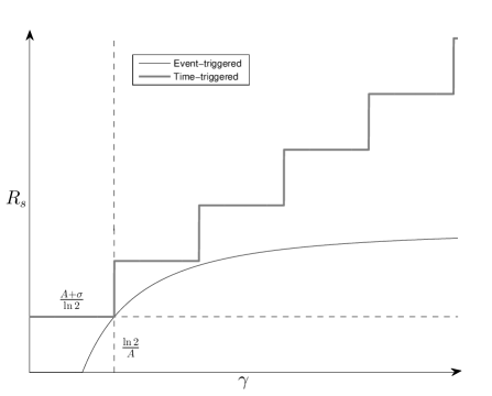
Figure 2: Illustration of the necessary bit rate for time-triggering control of a scalar plant (21) and approximation of the necessary bit rate for event-triggering control of a scalar plant (25) versus the worst-case delay in the communication channel. For the time-triggered scheme, $T=\ln 2/A$.

Figure 2 compares the results of Theorem 3 and Theorem 4. For small values of $\gamma$, the necessary transmission rate in Theorem 4 becomes, cf. [31],

$$R_{s}\geq 0.$$ (27)

On the other hand, the result of Theorem 3 in the scalar case and for small values of $\gamma$ can be written as

$$R_{s}\geq\frac{A+\sigma}{\ln 2}.$$ (28)

Comparing (27) and (28), the value of the intrinsic timing information in communication in an event-triggered design becomes evident. When the delay is small, the timing information carried by the triggering events is substantial and ensures that controller can stabilize the system. In contrast, for small values of the delay the information transmission rate required by a time-triggered implementation equals the information access rate required by the classic data-rate theorem.

For large delay values, it can be easily shown that while both the necessary and sufficient conditions for the event-triggered design in Theorems 4 and 5 converge to the asymptote $((A+\sigma)/\ln 2)(1+A/\sigma)$ as $\gamma\rightarrow\infty$, the time-triggered result in Theorem 3 for grows linearly as $\gamma\rightarrow\infty$. The reason for this difference is that the time-triggered design (19) depends only on the delay while the event-triggered scheme depends on both state and delay. In both time-triggered and event-triggered schemes the sensor does not have fore-knowledge of the delay, and the sensor needs to send larger packets when the worst-case delay is larger. On the other hand, the triggering rate in the event-triggering case tends to zero as $\gamma$ tends to infinity. More precisely, using Lemma 3 of [31] in the event-triggering setting for all of the possible realizations we have

$$t_{s}^{k+1}-t_{s}^{k}\geq\frac{-\ln(\rho_{0}e^{-\sigma\gamma})}{A+\sigma},$$

which tends to infinity as $\gamma\rightarrow\infty$. In contrast, in the time-triggered case for delay realization $\Delta_{k}=0$ for all $k\in\mathbb{N}$ we have

$$t_{s}^{k+1}-t_{s}^{k}=T,$$

and in this case the rate increases linearly with the delay. $\bullet$

V-C Necessary and sufficient transmission rate

We now extend the event-triggering results to the vector case.

Theorem 6

Consider the plant-sensor-channel-controller model described in Section II with plant dynamics (1), where all eigenvalues of $A$ are real and $A$ is equal to its Jordan block decomposition, estimator dynamics (4), event-triggering strategy (23), and packet sizes such that $z_{i}^{j}(t_{c,i}^{k,j})$ is determined at the controller within a ball of radius $\rho(t_{s,i}^{k,j})=\rho_{0}e^{-\sigma\gamma}v(t_{s,i}^{k,j})$ with $\nu$-precision. Then there exist a delay realization such that

$$R_{s}>\sum_{j=1}^{q}\frac{d_{j}(\lambda_{j}+\sigma)}{\ln\nu+\ln(2+\frac{e^{\sigma\gamma}}{\rho_{0}})}\max\left\{0,\log\frac{(e^{\lambda_{j}\gamma}-1)}{\rho_{0}e^{-\sigma\gamma}}\right\}.$$

Moreover, when $\sigma$ is sufficiently large the result can be approximated by

$$R_{s}>\sum_{j=1}^{q}\frac{d_{j}(\lambda_{j}+\sigma)}{\ln 2}\max\left\{0,1+\frac{\log(e^{\lambda_{j}\gamma}-1)}{-\log(\rho_{0}e^{-\sigma\gamma})}\right\}.$$

Theorem 7

Consider the plant-sensor-channel-controller model described in Section II with plant dynamics (1), where all eigenvalues of $A$ are real and $A$ is equal to its Jordan block decomposition, estimator dynamics (4), and event-triggering strategy (23). For the $j^{\text{th}}$ Jordan block choose the following sequence of design parameters

$$0<\rho_{1}^{j}<\ldots<\rho_{d_{j}-1}^{j}<\rho_{d_{j}}^{j}=\rho_{0}<1.$$

If the state estimation error satisfies $|z_{i}^{j}(0)|\leq v_{0,i}^{j}$, then we can achieve

$$|z_{i}^{j}(t)|\leq v_{0,i}^{j}((\rho_{0}-\rho_{i}^{j})+e^{(\lambda_{j}+\sigma)\gamma})e^{-\sigma t}$$

for $i=1,\ldots,d_{j}$ and $j=1,\ldots,q$, with an information transmission rate $R_{s}$ at least equal to

$$\sum_{j=1}^{j=q}\sum_{i=1}^{i=d_{j}}\frac{(\lambda_{j}+\sigma)}{-\ln(\rho_{i}^{j}e^{-\sigma\gamma})}\max\left(0,1+\log\frac{b\gamma(\lambda_{j}+\sigma)}{\ln(1+\rho_{i}^{j}e^{-(\sigma+\lambda_{j})\gamma})}\right),$$

where

$$0<v_{0,i}^{j}\leq\frac{v_{0,i-1}^{j}(\lambda_{j}+\sigma)(\rho_{0}-\rho_{i}^{j})}{((\rho_{0}-\rho_{i}^{j})+e^{(\lambda_{j}+\sigma)\gamma})(e^{(\lambda_{j}+\sigma)\gamma}-1)},$$ (29)

for $i=2,\ldots,d_{j}$ and $j=1,\ldots,q$, and $b>1$.

VI Conclusions

We investigated observability and stabilizability of a continuous-time scalar systems without disturbances in the presence of a finite rate digital communication channel subjected to unknown delay in the feedback loop. Our previous results about inherent information in event-triggered strategy have been extended to the vector case and compared with two time-triggered designs. Open problems for future research include studying the effect of system disturbances and obtaining exponential convergence guarantees for the stabilizability of the system.

References

- [1] K.-D. Kim and P. R. Kumar, “Cyber–physical systems: A perspective at the centennial,” Proceedings of the IEEE, vol. 100 (Special Centennial Issue), pp. 1287–1308, 2012.
- [2] K. Carruthers, “Internet of things and beyond: Cyber-physical systems,” Newsletter, vol. 2014, 2014.
- [3] S. Tatikonda and S. Mitter, “Control under communication constraints,” IEEE Transactions on Automatic Control, vol. 49, no. 7, pp. 1056–1068, 2004.
- [4] G. N. Nair and R. J. Evans, “Stabilizability of stochastic linear systems with finite feedback data rates,” SIAM Journal on Control and Optimization, vol. 43, no. 2, pp. 413–436, 2004.
- [5] N. C. Martins, M. A. Dahleh, and N. Elia, “Feedback stabilization of uncertain systems in the presence of a direct link,” IEEE Transactions on Automatic Control, vol. 51, no. 3, pp. 438–447, 2006.
- [6] P. Minero, M. Franceschetti, S. Dey, and G. N. Nair, “Data rate theorem for stabilization over time-varying feedback channels,” IEEE Transactions on Automatic Control, vol. 54, no. 2, p. 243, 2009.
- [7] P. Minero, L. Coviello, and M. Franceschetti, “Stabilization over Markov feedback channels: the general case,” IEEE Transactions on Automatic Control, vol. 58, no. 2, pp. 349–362, 2013.
- [8] R. T. Sukhavasi and B. Hassibi, “Linear time-invariant anytime codes for control over noisy channels,” IEEE Transactions on Automatic Control, vol. 61, no. 12, pp. 3826–3841, 2016.
- [9] E. Ardestanizadeh and M. Franceschetti, “Control-theoretic approach to communication with feedback,” IEEE Transactions on Automatic Control, vol. 57, no. 10, pp. 2576–2587, 2012.
- [10] J. Ding, Y. Peres, G. Ranade, and A. Zhai, “When multiplicative noise stymies control,” arXiv preprint arXiv:1612.03239, 2016.
- [11] C. De Persis, “n-bit stabilization of n-dimensional nonlinear systems in feedforward form,” IEEE Transactions on Automatic Control, vol. 50, no. 3, pp. 299–311, 2005.
- [12] D. Liberzon, “Nonlinear control with limited information,” Communications in Information & Systems, vol. 9, no. 1, pp. 41–58, 2009.
- [13] G. N. Nair, R. J. Evans, I. M. Mareels, and W. Moran, “Topological feedback entropy and nonlinear stabilization,” IEEE Transactions on Automatic Control, vol. 49, no. 9, pp. 1585–1597, 2004.
- [14] V. Kostina, Y. Peres, M. Z. Rácz, and G. Ranade, “Rate-limited control of systems with uncertain gain,” in 54th Annual Allerton Conference on Communication, Control and Computing, 2016.
- [15] Q. Ling and H. Lin, “Necessary and sufficient bit rate conditions to stabilize quantized Markov jump linear systems,” in Proceedings of the 2010 American Control Conference. IEEE, 2010, pp. 236–240.
- [16] G. Ranade and A. Sahai, “Control capacity,” in Information Theory (ISIT), 2015 IEEE International Symposium on. IEEE, 2015, pp. 2221–2225.
- [17] G. N. Nair, S. Dey, and R. J. Evans, “Communication-limited stabilisability of jump Markov linear systems,” in 15th Int. Symp. Mathematical Theory of Networks and Systems, Notre Dame, IN, 2002.
- [18] A. Sahai and S. Mitter, “The necessity and sufficiency of anytime capacity for stabilization of a linear system over a noisy communication link. Part I: Scalar systems,” IEEE transactions on Information Theory, vol. 52, no. 8, pp. 3369–3395, 2006.
- [19] A. S. Matveev and A. V. Savkin, Estimation and control over communication networks. Springer Science & Business Media, 2009.
- [20] M. Franceschetti and P. Minero, “Anytime capacity of a class of Markov channels,” IEEE Transactions on Automatic Control, 2016, in press.
- [21] G. Nair, “A non-stochastic information theory for communication and state estimation,” IEEE Transactions on Automatic Control, vol. 58, pp. 1497–1510, 2013.
- [22] M. Franceschetti and P. Minero, “Elements of information theory for networked control systems,” in Information and Control in Networks. Springer, 2014, pp. 3–37.
- [23] B. G. N. Nair, F. Fagnani, S. Zampieri, and R. J. Evans, “Feedback control under data rate constraints: An overview,” Proceedings of the IEEE, vol. 95, no. 1, pp. 108–137, 2007.
- [24] P. Tabuada, “Event-triggered real-time scheduling of stabilizing control tasks,” IEEE Transactions on Automatic Control, vol. 52, no. 9, pp. 1680–1685, 2007.
- [25] W. P. M. H. Heemels, K. H. Johansson, and P. Tabuada, “An introduction to event-triggered and self-triggered control,” in 51st IEEE Conference on Decision and Control (CDC). IEEE, 2012, pp. 3270–3285.
- [26] P. Tallapragada and J. Cortés, “Event-triggered stabilization of linear systems under bounded bit rates,” IEEE Transactions on Automatic Control, vol. 61, no. 6, pp. 1575–1589, 2016.
- [27] E. Kofman and J. H. Braslavsky, “Level crossing sampling in feedback stabilization under data-rate constraints,” in 45st IEEE Conference on Decision and Control (CDC). IEEE, 2006, pp. 4423–4428.
- [28] Q. Ling, “Bit rate conditions to stabilize a continuous-time scalar linear system based on event triggering,” IEEE Transactions on Automatic Control, 2016.
- [29] J. Pearson, J. P. Hespanha, and D. Liberzon, “Control with minimal cost-per-symbol encoding and quasi-optimality of event-based encoders,” IEEE Transactions on Automatic Control, 2016.
- [30] M. J. Khojasteh, P. Tallapragada, J. Cortés, and M. Franceschetti, “The value of timing information in event-triggered control: The scalar case,” in 54th Annual Allerton Conference on Communication, Control, and Computing. IEEE, 2016, pp. 1165–1172.
- [31] M. J. Khojasteh, P. Tallapragada, J. Cortés, and M. Franceschetti, “The value of timing information in event-triggered control,” arXiv preprint arXiv:1609.09594, 2016.
- [32] J. Hespanha, A. Ortega, and L. Vasudevan, “Towards the control of linear systems with minimum bit-rate,” in Proc. 15th Int. Symp. on Mathematical Theory of Networks and Systems (MTNS), 2002.
- [33] D. Liberzon and S. Mitra, “Entropy and minimal data rates for state estimation and model detection,” in Proceedings of the 19th International Conference on Hybrid Systems: Computation and Control. ACM, 2016, pp. 247–256.
- [34] V. V. Prasolov, Problems and theorems in linear algebra. American Mathematical Soc., 1994, vol. 134.