Explicit formulae for Chern-Simons invariants of the hyperbolic $J(2n,-2m)$ knot orbifolds

Abstract.

english

We calculate the Chern-Simons invariants of the hyperbolic double twist knot orbifolds using the Schläfli formula for the generalized Chern-Simons function on the family of cone-manifold structures of double twist knots.

1. Introduction

Chern-Simons invariants of hyperbolic knot orbifolds are computed explicitly for a few infinite families in [HL, HL2, HLMR] using the ‘‘Schläfli formula’’.

In this paper, we present the explicit formulae for Chern-Simons invariants of the hyperbolic double twist knot orbifolds and we present them numerically for some of double twist knot orbifolds. A brief history of Chern-Simons invariant can be found in [HL, HL2, HLMR]. A double twist knot is denoted by $C(2n,2m)$ according to Conway notation or by $J(2n,-2m)$ according to Hoste-Shanahan notation. Figure 2 presents $C(2n,2m)$ for $m,n>0$.

For a two-bridge hyperbolic link, there exists an angle $\alpha_{0}\in[\frac{2\pi}{3},\pi)$ for each link $K$ such that the cone-manifold $K(\alpha)$ is hyperbolic for $\alpha\in(0,\alpha_{0})$, Euclidean for $\alpha=\alpha_{0}$, and spherical for $\alpha\in(\alpha_{0},\pi]$ [P2, HLM1, K1, PW]. We will use the Chern-Simons invariant of the lens space $L\left(4nm+1,2n(2m-1)+1\right)$ calculated in [HLM2]. The following theorem gives the Chern-Simons invariant formulae for the hyperbolic $C(2n,2m)$ knots. Let $S_{k}(v)$ be the Chebychev polynomials defined by $S_{0}(v)=1$, $S_{1}(v)=v$ and $S_{k}(v)=vS_{k-1}(v)-S_{k-2}(v)$ for all integers $k$.

Theorem 1.1.

Let $X_{2n}^{2m}\!(\alpha)$ be the hyperbolic cone-manifold with underlying space $S^{3}$ and a singular set $C(2n,2m)$ of cone-angle $0\leq\alpha<\alpha_{0}$. Let $k$ be a positive integer such that $k$-fold cyclic covering of $X_{2n}^{2m}(\frac{2\pi}{k})$ is hyperbolic. Then the Chern-Simons invariant of $X_{2n}^{2m}(\frac{2\pi}{k})$ (mod $\frac{1}{k}$ if $k$ is even or mod $\frac{1}{2k}$ if $k$ is odd) is given by the following formula:

$$\text{{cs}}\left(X_{2n}^{2m}\left(\frac{2\pi}{k}\right)\right)\equiv\frac{1}{2}\text{{cs}}\left(L\left(4nm+1,2n(2m-1)+1\right)\right)$$

$$+\frac{1}{4\pi^{2}}\int_{\frac{2\pi}{k}}^{\alpha_{0}}Im\left(2*\log\left(-\frac{M^{2}(S_{n}(v)-S_{n-1}(v))-(S_{n-1}(v)-S_{n-2}(v))}{(S_{n}(v)-S_{n-1}(v))-M^{2}(S_{n-1}(v)-S_{n-2}(v))}\right)\right)\>d\alpha$$

$$+\frac{1}{4\pi^{2}}\int_{\alpha_{0}}^{\pi}Im\left(\log\left(-\frac{M^{2}(S_{n}(v_{1})-S_{n-1}(v_{1}))-(S_{n-1}(v_{1})-S_{n-2}(v_{1}))}{(S_{n}(v_{1})-S_{n-1}(v_{1}))-M^{2}(S_{n-1}(v_{1})-S_{n-2}(v_{1}))}\right)\right)\>d\alpha$$

$$+\frac{1}{4\pi^{2}}\int_{\alpha_{0}}^{\pi}Im\left(\log\left(-\frac{M^{2}(S_{n}(v_{2})-S_{n-1}(v_{2}))-(S_{n-1}(v_{2})-S_{n-2}(v_{2}))}{(S_{n}(v_{2})-S_{n-1}(v_{2}))-M^{2}(S_{n-1}(v_{2})-S_{n-2}(v_{2}))}\right)\right)\>d\alpha,$$

where for $M=e^{\frac{i\alpha}{2}}$, $x$ , $x_{1}$, and $x_{2}$ are zeroes of Riley-Mednykh polynomial $\phi_{2n}^{2m}(x,M)$ in Theorem 2.5. As $\alpha$ decreases to $\alpha_{0}$ both $x_{1}$ and $x_{2}$ approach a common value $x$. One of $x_{1}$ and $x_{2}$ comes from the component of $x$, and the other comes from the component of $\bar{x}$. $v$ satisfies $\text{{Im}}((S_{n}(v)-S_{n-1}(v))\overline{(S_{n-1}(v)-S_{n-2}(v))})\geq 0$ [Tran3, Lemma 3.9].

2. $C(2n,2m)$ knots

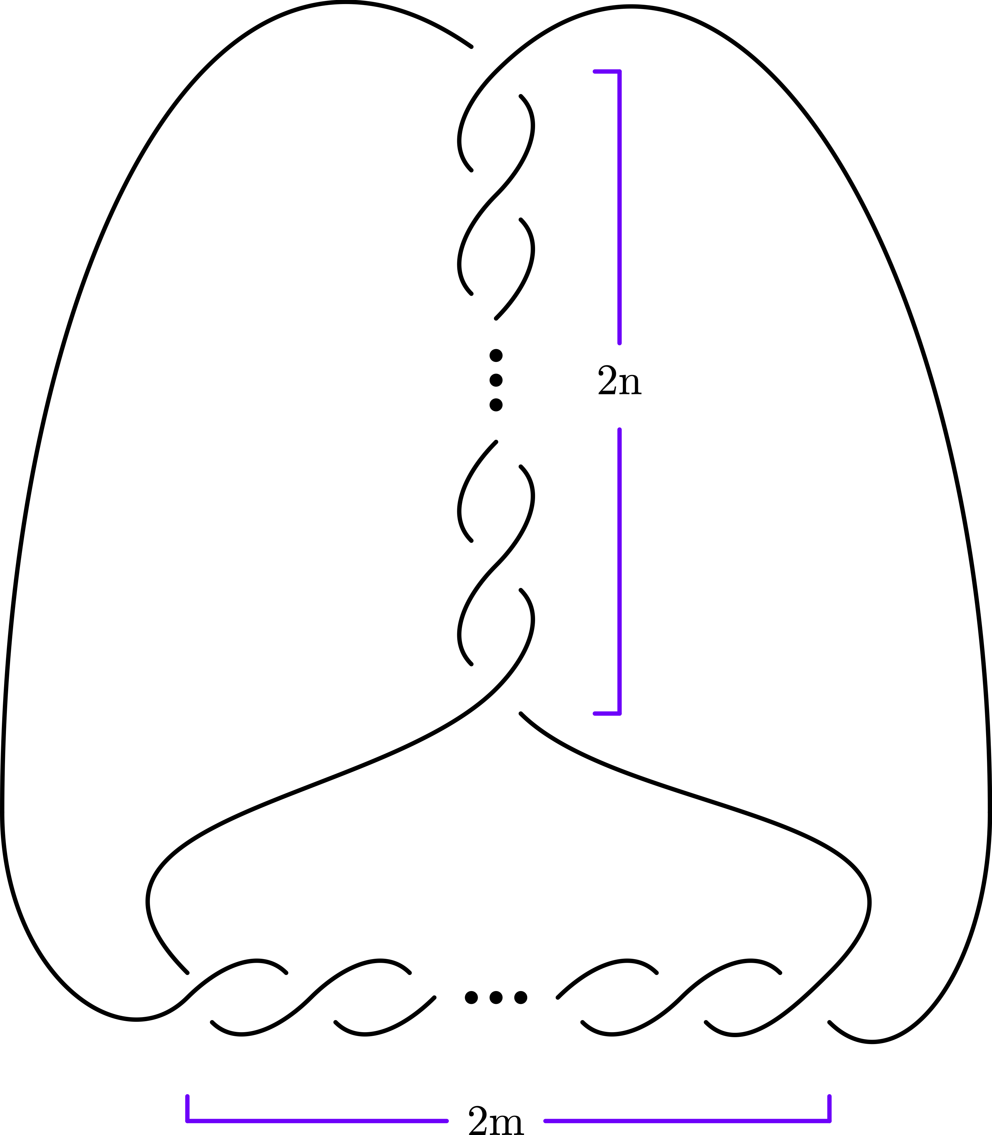
Figure 2.1. C(2n,2m)

A general reference for this section is  [HS]. A knot with $2n$ right-handed vertical crossings and $2m$ left-handed horizontal crossings as in Figure 2.1 is $C(2n,2m)$ knot according to Conway’s notation. One can easily check that the slope of $C(2n,2m)$ is $2m/(4nm+1)$ which is equivalent to the knot with slope $\left(2n(2m-1)+1\right)/(4nm+1)$ [S1].

We will use the following presentation of the fundamental group of $C(2n,2m)$ knot(equivalently, $J(2n,-2m)$ knot) in [HS]. In [HS], Hoste and Shanahan asked whether their presentation of the fundamental group for double twist knots can be derived from Schubert’s canonical 2-bridge diagram or not. The following proposition can also be obtained by reading off the fundamental group from the Schubert normal form of $C(2n,2m)$ with slope $2m/(4nm+1)$ [S1, R1] which answers Hoste-Shanahan’s question completely for $C(2n,2m)$ knots. Let$X_{2n}^{2m}$ be $S^{3}\backslash C(2n,2m)$.

Proposition 2.1.

[HLMR, Proposition2.2]  [R1, S1]

$$\pi_{1}(X_{2n}^{2m})=\left\langle s,t\ |\ sw^{m}t^{-1}w^{-m}=1\right\rangle,$$

where $w=(t^{-1}s)^{n}(ts^{-1})^{n}$.

2.2. The Chebychev polynomial

Let $S_{k}(v)$ be the Chebychev polynomials defined by $S_{0}(v)=1$, $S_{1}(v)=v$ and $S_{k}(v)=vS_{k-1}(v)-S_{k-2}(v)$ for all integers $k$. The following explicit formula for $S_{k}(v)$ can be obtained by solving the above recurrence relation [Tran2].

$$S_{n}(v)=\sum_{0\leq i\leq\lfloor\frac{n}{2}\rfloor}(-1)^{i}\binom{n-i}{i}v^{n-2i}$$

for $n\geq 0$, $S_{n}(v)=-S_{-n-2}(v)$ for $n\leq-2$, and $S_{-1}(v)=0$. The following proposition 2.3 can be proved using the Cayley-Hamilton theorem [Tran].

Proposition 2.3.

[Tran, Proposition 2.4] Suppose $V=\begin{bmatrix}a&b\\ c&d\end{bmatrix}\in\textnormal{SL}_{2}(\mathbb{C}).$ Then

$$V^{k}=\begin{bmatrix}S_{k}(v)-dS_{k-1}(v)&bS_{k-1}(v)\\ cS_{k-1}(v)&S_{k}(v)-aS_{k-1}(v)\end{bmatrix}$$

where $v=\textnormal{tr}(V)=a+d$.

2.4. The Riley-Mednykh polynomial

Let

$$\begin{array}[]{ccccc}\rho(s)=\left[\begin{array}[]{cc}M&1\\ 0&M^{-1}\end{array}\right]\text{,}\ \ \ \rho(t)=\left[\begin{array}[]{cc}M&0\\ 2-v&M^{-1}\end{array}\right],\end{array}$$

and let

$$\begin{array}[]{cc}c=\left[\begin{array}[]{cc}0&-\left(\sqrt{2-v}\right)^{-1}\\ \sqrt{2-v}&0\end{array}\right].\end{array}$$

Then from the above Proposition 2.3, we get the following Theorem 2.5. Let $\rho(s)=S$, $\rho(t)=T$ and $\rho(w)=W$. Then $\textnormal{tr}(T^{-1}S)=v=\textnormal{tr}(TS^{-1})$. Let $v=x+M^{2}+M^{-2}$. Theorem 2.5 can be found in [Tran3]. We include the proof for readers’ convenience.

Theorem 2.5.

[Tran3] $\rho$ is a representation of $\pi_{1}(X_{2n}^{2m})$ if and only if $x$ is a root of the following Riley-Mednykh polynomial,

$$\phi_{2n}^{2m}(x,M)=S_{m}(z)+\left[-1+xS_{n-1}(v)\left(S_{n}(v)+(1-v)S_{n-1}(v)\right)\right]S_{m-1}(z).$$

• Since

  $$T^{-1}S =\left[\begin{array}[]{cc}1&M^{-1}\\ M(M^{-2}+(x-2)+M^{2})&M^{-2}+x-1+M^{2}\end{array}\right]\text{ and}$$

  $$TS^{-1} =\left[\begin{array}[]{cc}1&-M\\ -M^{-1}(M^{-2}+(x-2)+M^{2})&M^{-2}+x-1+M^{2}\end{array}\right],$$

  $$(T^{-1}S)^{n} =\left[\begin{array}[]{cc}S_{n}(v)-(v-1)S_{n-1}(v)&M^{-1}S_{n-1}(v)\\ M(v-2)S_{n-1}(v)&S_{n}(v)-S_{n-1}(v)\end{array}\right],$$

  $$(TS^{-1})^{n} =\left[\begin{array}[]{cc}S_{n}(v)-(v-1)S_{n-1}(v)&-MS_{n-1}(v)\\ -M^{-1}(v-2)S_{n-1}(v)&S_{n}(v)-S_{n-1}(v)\end{array}\right]$$

Hence

$$W=(T^{-1}S)^{n}(TS^{-1})^{n}=\begin{bmatrix}W_{11}&W_{12}\\ (2-v)W_{12}&W_{22}\end{bmatrix}\ \text{where}$$

$$W_{11} =S^{2}_{n}(v)+(2-2v)S_{n}(v)S_{n-1}(v)+(1+2M^{-2}-2v-M^{-2}v+v^{2})S^{2}_{n-1}(v)$$

$$W_{12} =(M^{-1}-M)S_{n}(v)S_{n-1}(v)+(Mv-M-M^{-1})S^{2}_{n-1}(v)$$

$$W_{22} =S^{2}_{n}(v)-2S_{n}(v)S_{n-1}(v)+(1+2M^{2}-M^{2}v)S^{2}_{n-1}(v).$$

Let $z=\text{Tr}(W)$. Then, since $S_{n}^{2}(v)-vS_{n}(v)S_{n-1}(v)+S_{n-1}^{2}(v)=1$ (by [Tran1, Lemma 2.1] or by induction),

$$z=W_{11}+W_{22} =2(S^{2}_{n}(v)-vS_{n}(v)S_{n-1}(v)+S^{2}_{n-1}(v))$$

$$+(2M^{-2}+2M^{2}-2v-M^{-2}v-M^{2}v+v^{2})S^{2}_{n-1}(v)$$

$$=2+(v-2)xS^{2}_{n-1}(v).$$

By Proposition 2.3, we have

$$(W)^{m} =\left[\begin{array}[]{cc}S_{m}(z)-W_{22}S_{m-1}(z)&W_{12}S_{m-1}(z)\\ (2-v)W_{12}S_{m-1}(z)&S_{m}(z)-W_{11}S_{m-1}(z)\end{array}\right].$$

Therefore

$$\textnormal{tr}(SW^{m}c)/\sqrt{2-v}\left(=(M-M^{-1})W_{12}S_{m-1}(z)+S_{m}(z)-W_{11}S_{m-1}(z)\right)$$

gives $\phi_{2n}^{2m}(x,M)$ [HLMR]. ∎

3. Longitude

Let $l=w^{m}(w^{*})^{m}$, where $w^{*}$ is the word obtained by reversing $w$. Then $l$ is the longitude which is null-homologus in $X_{2n}^{2m}$. Recall $\rho(w)=W$. Let $\widetilde{W}=\rho(w^{*})$. It is easy to see that $\widetilde{W}$ can be written as

$$\widetilde{W}=\begin{bmatrix}\tilde{W}_{22}&\tilde{W}_{12}\\ (2-v)\tilde{W}_{12}&\tilde{W}_{11}\end{bmatrix}$$

where $\tilde{W}_{ij}$ is obtained by $W_{ij}$ by replacing $M$ with $M^{-1}$. Similar computation was introduced in [HS]. Hence,

$$\tilde{W}_{11} =S^{2}_{n}(v)+(2-2v)S_{n}(v)S_{n-1}(v)+(1+2M^{2}-2v-M^{2}v+v^{2})S^{2}_{n-1}(v)$$

$$\tilde{W}_{12} =(M-M^{-1})S_{n}(v)S_{n-1}(v)+(M^{-1}v-M^{-1}-M)S^{2}_{n-1}(v)$$

$$\tilde{W}_{22} =S^{2}_{n}(v)-2S_{n}(v)S_{n-1}(v)+(1+2M^{-2}-M^{-2}v)S^{2}_{n-1}(v).$$

The following lemma was introduced in [HS] with slightly different coordinates.

Let $L=\rho(l)_{11}$(the left upper entry of $\rho(l)$).

Lemma 3.1.

[HS] $W_{21}L+\tilde{W}_{21}=0$.

Theorem 3.2.

$$L=-\frac{M^{2}(S_{n}(v)-S_{n-1}(v))-(S_{n-1}(v)-S_{n-2}(v))}{(S_{n}(v)-S_{n-1}(v))-M^{2}(S_{n-1}(v)-S_{n-2}(v))}.$$

• By directly computing $W_{21}L+\tilde{W}_{21}=0$ in Lemma 3.1 and substituting $S_{n}(v)+S_{n-2}(v)$ for $vS_{n-1}(v)$, the theorem follows. ∎

4. Schläfli formula for the generalized Chern-Simons function

The general references for this section are [HLM3, HLM2, Y1, MeyRub1, HL, HL2] and [HLMR].

In [HLM3], Hilden, Lozano, and Montesinos-Amilibia defined the generalized Chern-Simons function on the oriented cone-manifold structures which matches up with the Chern-Simons invariant when the cone-manifold is the Riemannian manifold.

Below, we briefly introduce the generalized Chern-Simons function on the family of $C(2n,2m)$ cone-manifold structures. For an oriented knot $C(2n,2m)$, we orient its chosen meridian $s$ such that the orientation of $s$ followed by the orientation of $C(2n,2m)$ coincides with orientation of $\mathbb{S}^{3}$. Here, we use the definition of the lens space in [HLM2] so that we can have the right orientation when it is combined with the following frame field. On the Riemannian manifold $\mathbb{S}^{3}-C(2n,2m)-s$ we choose a special frame field $\Gamma=(e_{1},e_{2},e_{3})$ which is an orthonormal frame field such that for each point $x$ near $C(2n,2m)$, $e_{1}(x)$ has the direction given by knot’s orientation, $e_{2}(x)$ has the tangent direction of the meridian curve, and $e_{3}(x)$ has the knot to point $x$ direction. Such a special frame field always exists by Proposition $3.1$ of [HLM3]. From $\Gamma$ we obtain an orthonormal frame field $\Gamma_{\alpha}$ on $X_{2n}^{2m}\!(\alpha)-s$ by the Gram-Schmidt orthogonalization process with respect to the Riemannian structure of the cone manifold $X_{2n}^{2m}\!(\alpha)$. Moreover, it can be made special by deforming it in a neighbourhood of the singular set $C(2n,2m)$ and $s$, if necessary. Thus, $\Gamma^{\prime}$ is an extension of $\Gamma$ to $S^{3}-C(2n,2m)$. To the cone-manifold $X_{2n}^{2m}\!(\alpha)$, we assign a real number

$$I\left(X_{2n}^{2m}\!(\alpha)\right)=\frac{1}{2}\int_{\Gamma(S^{3}-T_{2n}-s)}Q-\frac{1}{4\pi}\tau(s,\Gamma^{\prime})-\frac{1}{4\pi}\left(\frac{\beta\alpha}{2\pi}\right),$$

where $-2\pi\leq\beta\leq 2\pi$ is the angle of the lifted holonomy of the singular locus of $X_{2n}^{2m}\!(\alpha)$, $Q$ is the Chern-Simons form:

$$Q=\frac{1}{4\pi^{2}}\left(\theta_{12}\wedge\theta_{13}\wedge\theta_{23}+\theta_{12}\wedge\Omega_{12}+\theta_{13}\wedge\Omega_{13}+\theta_{23}\wedge\Omega_{23}\right),$$

and

$$\tau(s,\Gamma^{\prime})=-\int_{\Gamma^{\prime}(s)}\theta_{23},$$

where ($\theta_{ij}$) is the connection $1$-form, ($\Omega_{ij}$) is the curvature $2$-form of the Riemannian connection on $X_{2n}^{2m}\!(\alpha)$ and the integral is over the orthonormalizations of the same frame field. When $\alpha=\frac{2\pi}{k}$ for some positive integer, $I\left(X_{2n}^{2m}\!\!\left(\frac{2\pi}{k}\right)\right)$ (mod $\frac{1}{k}$ if $k$ is even or mod $\frac{1}{2k}$ if $k$ is odd) is independent of the frame field $\Gamma$ and of the representative in the equivalence class $\overline{\beta}$ and hence becomes an invariant of the orbifold $X_{2n}^{2m}\!\!\left(\frac{2\pi}{k}\right)$. The quantity $I\left(X_{2n}^{2m}\!\!\left(\frac{2\pi}{k}\right)\right)$ (mod $\frac{1}{k}$ if $k$ is even or mod $\frac{1}{2k}$ if $k$ is odd) is called the Chern-Simons invariant of the orbifold and is denoted by $\text{{cs}}\left(X_{2n}^{2m}\!\!\left(\frac{2\pi}{k}\right)\right)$.

We have the following ‘‘Schläfli formula’’ for the generalized Chern-Simons function on the family of $C(2n,2m)$ cone-manifold structures.

Theorem 4.1.

( [HLM2, Theorem 1.2])  For a family of geometric cone-manifold structures, $X_{2n}^{2m}\!(\alpha)$, and differentiable functions $\alpha(t)$ and $\beta(t)$ of $t$ we have

$$dI\left(X_{2n}^{2m}\!(\alpha)\right)=-\frac{1}{4\pi^{2}}\beta d\alpha.$$

5. Proof of the theorem 1.1

For $n\geq 1$ and $M=e^{i\frac{\alpha}{2}}$, $\phi_{2n}^{2m}(x,M)$ have $2mn$ component zeros. The component which passes through

$$(x_{1},x_{2})=\left(2-2\cos{\left(\frac{\pi(2m+1)}{4nm+1}\right)},2-2\cos{\left(\frac{\pi(2m-1)}{4nm+1}\right)}\right)$$

at $\alpha=\pi$ is the geometric component by  [HLM2, Theorem 2.1]. Note that $2-x_{1}>0$ and $2-x_{2}>0$. For each $C(2n,2m)$, there exists an angle $\alpha_{0}\in[\frac{2\pi}{3},\pi)$ such that $C(2n,2m)$ is hyperbolic for $\alpha\in(0,\alpha_{0})$, Euclidean for $\alpha=\alpha_{0}$, and spherical for $\alpha\in(\alpha_{0},\pi]$ [P2, HLM1, K1, PW]. Denote by $D(X_{2n}^{2m}\!(\alpha))$ be the set of zeros of the discriminant of $\phi_{2n}^{2m}(x,e^{i\frac{\alpha}{2}})$ over $x$. Then $\alpha_{0}$ will be one of $D(X_{2n}^{2m}\!(\alpha))$.

On the geometric component we can calculate the Chern-Simons invariant of an orbifold $X_{2n}^{2m}(\frac{2\pi}{k})$ (mod $\frac{1}{k}$ if $k$ is even or mod $\frac{1}{2k}$ if $k$ is odd), where $k$ is a positive integer such that $k$-fold cyclic covering of $X_{2n}^{2m}(\frac{2\pi}{k})$ is hyperbolic:

$$\text{{cs}}\left(X_{2n}^{2m}\left(\frac{2\pi}{k}\right)\right)\equiv I\left(X_{2n}^{2m}\left(\frac{2\pi}{k}\right)\right)\ \ \ \ \ \ \ \ \ \ \ \ \left(\text{mod}\ \frac{1}{k}\right)$$

$$\equiv I\left(X_{2n}^{2m}(\pi)\right)+\frac{1}{4\pi^{2}}\int_{\frac{2\pi}{k}}^{\pi}\beta\>d\alpha\ \ \ \ \ \ \ \ \ \ \ \ \ \ \ \ \ \ \ \ \left(\text{mod}\ \frac{1}{k}\right)$$

$$\equiv\frac{1}{2}\text{{cs}}\left(L(4nm+1,2n(2m-1)+1)\right)$$

$$+\frac{1}{4\pi^{2}}\int_{\frac{2\pi}{k}}^{\alpha_{0}}Im\left(2*\log\left(-\frac{M^{2}(S_{n}(v)-S_{n-1}(v))-(S_{n-1}(v)-S_{n-2}(v))}{(S_{n}(v)-S_{n-1}(v))-M^{2}(S_{n-1}(v)-S_{n-2}(v))}\right)\right)\>d\alpha$$

$$+\frac{1}{4\pi^{2}}\int_{\alpha_{0}}^{\pi}Im\left(\log\left(-\frac{M^{2}(S_{n}(v_{1})-S_{n-1}(v_{1}))-(S_{n-1}(v_{1})-S_{n-2}(v_{1}))}{(S_{n}(v_{1})-S_{n-1}(v_{1}))-M^{2}(S_{n-1}(v_{1})-S_{n-2}(v_{1}))}\right)\right)\>d\alpha$$

$$+\frac{1}{4\pi^{2}}\int_{\alpha_{0}}^{\pi}Im\left(\log\left(-\frac{M^{2}(S_{n}(v_{2})-S_{n-1}(v_{2}))-(S_{n-1}(v_{2})-S_{n-2}(v_{2}))}{(S_{n}(v_{2})-S_{n-1}(v_{2}))-M^{2}(S_{n-1}(v_{2})-S_{n-2}(v_{2}))}\right)\right)\>d\alpha$$

$$\left(\text{mod}\ \frac{1}{k}\ \text{if $k$ is even or }\text{mod}\ \frac{1}{2k}\ \text{if $k$ is odd}\right)$$

where the second equivalence comes from Theorem 4.1 and the third equivalence comes from the fact that $I\left(X_{2n}^{2m}(\pi)\right)\equiv\frac{1}{2}\text{{cs}}\left(L(4nm+1,2n(2m-1)+1)\right)$ $\left(\text{mod }\frac{1}{2}\right)$, Theorem 3.2, and geometric interpretations of hyperbolic and spherical holonomy representations.

The following theorem gives the Chern-Simons invariant of the Lens space $L(4nm+1,2n(2m-1)+1)$.

Theorem 5.1.

( [HLM2, Theorem 1.3])

$$\text{{cs}}\left(L\left(4nm+1,2n(2m-1)+1\right)\right)\equiv\frac{m-n}{4nm+1} (\text{mod}\ 1).$$

6. Chern-Simons invariants of the hyperbolic $C(2n,2m)$ knot orbifolds and of its cyclic coverings

The table 6.1 gives the approximate Chern-Simons invariant of $C(2n,2m)$ for $n$ between $1$ and $4$, $m$ between $1$ and $4$ with $n\geq m$. Since $C(2,2)$, $C(4,4)$, $C(6,6)$, $C(8,8)$ are amphicheiral knots, their Chern-Simons invariants are $zero$ as expected. We used Simpson’s rule for the approximation with $2\times 10^{4}$ ($10^{4}$ in Simpson’s rule) intervals from $0$ to $\alpha_{0}$ and $2\times 10^{4}$ ($10^{4}$ in Simpson’s rule) intervals from $\alpha_{0}$ to $\pi$. The table 6.2 gives the approximate Chern-Simons invariant of the hyperbolic orbifold, $\text{{cs}}\left(X_{2n}^{2m}(\frac{2\pi}{k})\right)$ for $n$ between $1$ and $4$, $m$ between $1$ and $4$ with $n\geq m$, and for $k$ between $3$ and $10$, and of its cyclic covering, $\text{{cs}}\left(M_{k}(X_{2n}^{2m})\right)$ except amphicheiral knots. We used Simpson’s rule for the approximation with $2\times 10^{2}$ ($10^{2}$ in Simpson’s rule) intervals from $2\pi/k$ to $\alpha_{0}$ and $2\times 10^{2}$ ($10^{2}$ in Simpson’s rule) intervals from $\alpha_{0}$ to $\pi$.

We used Mathematica for the calculations. We record here that our data in Table 6.1 and those obtained from SnapPy [SnapPy] match up up to existing decimal points and our data in Table 6.2. For computational reasons, we need $\alpha_{0}$. $\alpha_{0}$ is the bifercation point of the geometric solution of the Riley-Mednykh polynomial as described in Theorem 1.1.

2n	2m	$\alpha_{0}$	$\text{{cs}}\left(X_{2n}^{2m}\right)$
2	2	2.094395102393195	0
4	2	2.574140778131840	0.34402298
6	2	2.750685152010280	0.27786688
8	2	2.843209532683532	0.24222232
4	4	2.847642272262783	0
6	4	2.942465754372979	0.42782933
8	4	2.990939179603150	0.38923730
6	6	3.007517657179940	0
8	6	3.040474611156828	0.46103929
8	8	3.065453796328835	0

Table 6.1. Chern-Simons invariant of $X_{2n}^{2m}$ for $n$ between $1$ and $4$, $m$ between $1$ and $4$ with $n\geq m$ except amphicheiral knots.

$k$ $\text{{cs}}\left(X_{4}^{2}(\frac{2\pi}{k})\right)$ $\text{{cs}}\left(M_{k}(X_{4}^{2})\right)$ 3 0.0875301 0.26259 4 0.144925 0.579699 5 0.0784576 0.392288 6 0.0351571 0.210943 7 0.00506505 0.0354553 8 0.108039 0.864313 9 0.0218112 0.196301 10 0.0530574 0.530574

$k$ $\text{{cs}}\left(X_{6}^{2}(\frac{2\pi}{k})\right)$ $\text{{cs}}\left(M_{k}(X_{6}^{2})\right)$ 3 0.0449535 0.13486 4 0.0876043 0.350417 5 0.0165337 0.0826684 6 0.138167 0.829004 7 0.0120078 0.0840545 8 0.0430876 0.3447 9 0.012125 0.109125 10 0.0876213 0.876213

$k$ $\text{{cs}}\left(X_{8}^{2}(\frac{2\pi}{k})\right)$ $\text{{cs}}\left(M_{k}(X_{8}^{2})\right)$ 3 0.0161266 0.0483799 4 0.0536832 0.214733 5 0.0817026 0.408513 6 0.103012 0.618074 7 0.0481239 0.336867 8 0.00768503 0.0614802 9 0.032221 0.289989 10 0.0521232 0.521232

$k$ $\text{{cs}}\left(X_{6}^{4}(\frac{2\pi}{k})\right)$ $\text{{cs}}\left(M_{k}(X_{6}^{4})\right)$ 3 0.125912 0.377736 4 0.192764 0.771058 5 0.0360431 0.180216 6 0.0996796 0.598077 7 0.00284328 0.0199029 8 0.0554674 0.443739 9 0.0409685 0.368717 10 0.0294401 0.294401

$k$ $\text{{cs}}\left(X_{8}^{4}(\frac{2\pi}{k})\right)$ $\text{{cs}}\left(M_{k}(X_{8}^{4})\right)$ 3 0.098074 0.294222 4 0.157843 0.631371 5 0.0993608 0.496804 6 0.0622858 0.373715 7 0.0365103 0.255572 8 0.0174882 0.139906 9 0.00284881 0.0256393 10 0.091224 0.91224

$k$ $\text{{cs}}\left(X_{8}^{6}(\frac{2\pi}{k})\right)$ $\text{{cs}}\left(M_{k}(X_{8}^{6})\right)$ 3 0.138854 0.416562 4 0.214725 0.858898 5 0.0628859 0.31443 6 0.128841 0.773046 7 0.0332457 0.23272 8 0.0866094 0.692875 9 0.0170324 0.153291 10 0.0613865 0.613865

Table 6.2. Chern-Simons invariant of the hyperbolic orbifold, $\text{{cs}}\left(X_{2n}^{2m}(\frac{2\pi}{k})\right)\left(\text{mod}\ \frac{1}{k}\ \text{if $k$ is even or }\text{mod}\ \frac{1}{2k}\ \text{if $k$ is odd}\right)$ for $n$ between $1$ and $4$, $m$ between $1$ and $4$ with $n\geq m$, and for $k$ between $3$ and $10$, and of its cyclic covering, $\text{{cs}}\left(M_{k}(X_{2n}^{2m})\right)$ except amphicheiral knots.

Note that the Chern-Simons invariant of the hyperbolic orbifold $\text{{cs}}\left(X_{2n}^{2m}(\frac{2\pi}{k})\right)$ is only defined modulo $\frac{1}{k}$ [HLM2, Theorem 1.4] and we only get modulo $\frac{1}{2k}$ for $k$ odd [HLM2, Theorem 1.4].

References

• [1] Marc Culler, Nathan Dunfield, Jeff Weeks, Many others. SnapPy. http://www.math.uic.edu/t3m/SnapPy/.
• [2] Ji-Young Ham, Joongul Lee. Explicit formulae for Chern-Simons invariants of the twist-knot orbifolds and edge polynomials of twist knots. Mat. Sb., 207(9):144–160, 2016.
• [3] Ji-Young Ham, Joongul Lee. Explicit formulae for Chern-Simons invariants of the hyperbolic orbifolds of the knot with Conway’s notation $C(2n,3)$. Lett. Math. Phys., 107(3):427–437, 2017.
• [4] Ji-Young Ham, Joongul Lee, Alexander Mednykh, Aleksei Rasskazov. On the volume and Chern-Simons invariant for 2-bridge knot orbifolds. J. Knot Theory Ramifications, 26(12):1750082, 22, 2017.
• [5] Hugh Hilden, MarΓ­aΒ Teresa Lozano, José MarΓ­a Montesinos-Amilibia. On a remarkable polyhedron geometrizing the figure eight knot cone manifolds. J. Math. Sci. Univ. Tokyo, 2(3):501–561, 1995.
• [6] HughΒ M. Hilden, MarΓ­aΒ Teresa Lozano, José MarΓ­a Montesinos-Amilibia. On volumes and Chern-Simons invariants of geometric $3$-manifolds. J. Math. Sci. Univ. Tokyo, 3(3):723–744, 1996.
• [7] HughΒ M. Hilden, MarΓ­aΒ Teresa Lozano, José MarΓ­a Montesinos-Amilibia. Volumes and Chern-Simons invariants of cyclic coverings over rational knots. In Topology and TeichmΓΌller spaces (Katinkulta, 1995), 31–55. World Sci. Publ., River Edge, NJ, 1996.
• [8] Jim Hoste, PatrickΒ D. Shanahan. A formula for the A-polynomial of twist knots. J. Knot Theory Ramifications, 13(2):193–209, 2004.
• [9] Sadayoshi Kojima. Deformations of hyperbolic $3$-cone-manifolds. J. Differential Geom., 49(3):469–516, 1998.
• [10] Robert Meyerhoff, Daniel Ruberman. Mutation and the $\eta$-invariant. J. Differential Geom., 31(1):101–130, 1990.
• [11] Joan Porti. Spherical cone structures on 2-bridge knots and links. Kobe J. Math., 21(1-2):61–70, 2004.
• [12] Joan Porti, Hartmut Weiss. Deforming Euclidean cone 3-manifolds. Geom. Topol., 11:1507–1538, 2007.
• [13] Robert Riley. Parabolic representations of knot groups. I. Proc. London Math. Soc. (3), 24:217–242, 1972.
• [14] Horst Schubert. Knoten mit zwei BrΓΌcken. Math. Z., 65:133–170, 1956.
• [15] AnhΒ T. Tran. Reidemeister torsion and Dehn surgery on twist knots. Tokyo J. Math., 39(2):517–526, 2016.
• [16] AnhΒ T. Tran. Volumes of hyperbolic double twist knot cone-manifolds. J. Knot Theory Ramifications, 26(11):1750068, 14, 2017.
• [17] AnhΒ T. Tran. The A-polynomial 2-tuple of twisted Whitehead links. Internat. J. Math., 29(2):1850013, 14, 2018.
• [18] AnhΒ T. Tran. Twisted Alexander polynomials of genus one two-bridge knots. Kodai Math. J., 41(1):86–97, 2018.
• [19] Tomoyoshi Yoshida. The $\eta$-invariant of hyperbolic $3$-manifolds. Invent. Math., 81(3):473–514, 1985.