Abstract

In this thesis, we obtain the formula for the Kac determinant of the algebra arising from the level $N$ representation of the Ding-Iohara-Miki algebra. This formula can be proved by decomposing the level $N$ representation into the deformed $W$-algebra part and the $U(1)$ boson part, and using the screening currents of the deformed $W$-algebra. It is also discovered that singular vectors obtained by its screening currents correspond to the generalized Macdonald functions. Moreover, we investigate the $q\rightarrow 0$ limit of five-dimensional AGT correspondence. In this limit, the simplest 5D AGT conjecture is proved, that is, the inner product of the Whittaker vector of the deformed Virasoro algebra coincides with the partition function of the 5D pure gauge theory. Furthermore, the R-Matrix of the Ding-Iohara-Miki algebra is explicitly calculated, and its general expression in terms of the generalized Macdonald functions is conjectured.

 

Singular Vector of Ding-Iohara-Miki Algebra and Hall-Littlewood Limit of 5D AGT Conjecture

Yusuke Ohkubo

1 Introduction

1.1. The Jack symmetric polynomials [1, 2] are a system of orthogonal polynomials expressing the excited states of an integrable one-dimensional quantum many-body system with the trigonometric type potential called the Calogero-Sutherland model [3, 4]. These are one-parameter deformations of the Schur symmetric polynomials. In general, being integrable means that the model has sufficiently many conserved quantities, and that system can be analytically solved. Like the Calogero-Sutherland model, many of the integrable systems are not physical models of particles existing in the real world. However, the mathematical structure of the integrable models, e.g., excellent solvability, can be used to advantage in many fields of mathematics.

Let us consider symmetric functions which are defined as a projective limit of symmetric polynomials with finite variables [5, Chap. 1]. In the case of the Jack polynomials, the infinite-variable limit exists and is called the Jack symmetric functions. The Jack functions are parametrized by partitions or Young diagrams, and has the complex parameter $\beta$ (see also Footnote 1). Actually we can consider the parameter $\beta$ as an indeterminate, and then the Jack functions are defined over the field $\mathbb{Q}(\beta)$. The surprising result due to Mimachi and Yamada is that the Jack functions associated to rectangular Young diagrams have a one-to-one correspondence with singular vectors of the Virasoro algebra [6]. The Virasoro algebra is constructed by the infinitesimal conformal transformations in two dimensions, and is the Lie algebra generated by $L_{n}$（$n\in\mathbb{Z}$） and the central element $c$ satisfying the relations

$$[L_{n},L_{m}]=(n-m)L_{n+m}+c\>\frac{n(n^{2}-1)}{12}\delta_{n+m,0},\quad n,m\in\mathbb{Z},$$ (1.1)

$$[L_{n},c]=0,\quad n\in\mathbb{Z}.$$ (1.2)

This is an essential algebra to two-dimensional conformal field theories required for string theory and statistical mechanics. To obtain the irreducible representations of the Virasoro algebra is important not only in representation theory but also in the conformal field theories. The irreducibility of highest weight representations can be determined by special vectors called singular vectors in the highest weight representation. Although the singular vectors have an integral representation, the expression formula of the Jack functions by the Dunkl operator [7] is more useful. Further, various properties of Jack functions are known. Thus, the expression of the singular vectors by the Jack functions is very convenient and beneficial.

As a $q$-difference deformation of the Jack polynomials, there is a system of orthogonal polynomials with rich theory called the Macdonald polynomials [5]. For later use let us introduce the notation for Macdonald symmetric function, which is the infinite-variable version of the Macdonald polynomial. We denote by $P_{\lambda}(p_{n};q,t)$ the Macdonald symmetric function associated to the partition $\lambda$. Here $q$ and $t$ are free parameters, and they can be considered as complex numbers or indeterminates. In this paper, we regard the power sum symmetric functions $p_{n}$ as variables of the Macdonald functions (for more detail, see Appendix A). The Macdonald polynomials are also simultaneous eigen-functions of commuting $q$-difference operators, now called Macdonald difference operators. Let us also mention that they are related to the Ruijsenaars model [8] which is a relativistic extension of the Calogero-Sutherland model. The $q$-deformation like the Macdonald functions makes theory clearer and often mathematically easier to handle. For example, the Jack functions can be characterized as the Hamiltonian $H_{\beta}$ (see Footnote 1), but they have ​​degenerate eigenvalues, and difficulties arise when we prove their orthogonality and ​​coincidence with the singular vectors. In the theory of the Macdonald functions, this degeneracy problem can be eliminated and the discussion is clearer. Also, the Hamiltonian $H_{\beta}$ has an infinite number of commuting operators. However, it is difficult to write down these operators explicitly [9], and in the Macdonald theory we have an explicit formula for the commuting family of difference operators having $P_{\lambda}(p_{n};q,t)$ as simultaneous eigenfunctions. For the above reason, it can be said that Macdonald’s theory is more beautiful.

In the $q\rightarrow 1$ ($t=q^{\beta}$) limit with $\beta$ fixed, the Macdonald functions are reduced to the Jack functions. On the other hand, in $q\rightarrow 0$ limit with $t$ fixed, they are reduced to the symmetric functions called the Hall-Littlewood functions. The Hall-Littlewood functions have a close connection to the character of the general linear group over finite fields, and they are also a generalization of the Schur functions [5, Chap. III]. It is one of the advantages that it is possible to unify and generalize the two generalizations of the Schur functions. Some applications in knot invariants [10, 11, 12] and stochastic processes [13] are also known. The Macdonald functions are one of the important symmetric functions for modern mathematics.

Awata, Kubo, Odake and Shiraishi introduced in [14] a $q$-deformation of the Virasoro algebra, which is named the deformed Virasoro algebra. This deformed algebra is designed so that singular vectors of Verma modules correspond to Macdonald symmetric functions $P_{\lambda}(p_{n};q,t)$. The deformed Virasoro algebra is an associative algebra defined over the base field $\mathbb{Q}(q,t)$, where $q$ and $t$ are the same parameters as in $P_{\lambda}(p_{n};q,t)$. The generators are denoted by $T_{n}$ ($n\in\mathbb{Z}$), and the defining relation is

$$[T_{n},T_{m}]=-\sum_{l=1}^{\infty}f_{l}(T_{n-l}T_{m+l}-T_{m-l}T_{n+l})-\frac{(1-q)(1-t^{-1})}{1-p}(p^{n}-p^{-n})\delta_{n+m,0},$$ (1.3)

where $p\mathbin{:=}q/t$ and $f_{l}$ are the structure constants defined by

$$f(z)=\sum_{l=0}^{\infty}f_{l}\>z^{l}\mathbin{:=}\exp\left(\sum_{n=1}^{\infty}\frac{1}{n}\frac{(1-q^{n})(1-t^{-n})}{1+p^{n}}z^{n}\right).$$ (1.4)

It is shown that the singular vectors of the deformed Virasoro algebra coincide with the Macdonald functions associated with rectangular Young diagrams. It is also possible to obtain the Jack and Macodnald functions associated with general partitions from the singular vectors of the $W_{N}$-algebra and the deformed $W_{N}$-algebra (which is the (deformed) Virasoro algebra when $N=2$) [15, 16, 17]. To be exact, singular vectors of the (deformed) $W_{N}$-algebra can be realized by $N-1$ families of bosons under the free field representation. By a certain projection to one of these bosons, we can obtain the Jack (or Macdonald) functions associated with Young diagrams with $N-1$ edges (see Figure 1).

Figure 1: Young diagram with $N-1$ edges

1.2. The representation theory of the Virasoro algebra plays an essential role in the two-dimensional conformal field theories. In 2009, while studying the low energy effective theory of M5-branes, Alday, Gaiotto and Tachikawa discovered the correspondence between the correlation functions of two-dimensional conformal field theories and the partition functions of four-dimensional supersymmetric gauge theories (AGT conjecture) [18]. Gauge theory has a long history and is an attractive theory studied by a lot of mathematicians and physicists. Although it is difficult to calculate the partition functions of gauge theories in general, Nekrasov gave an explicit formula (Nekrasov formula) for the instanton partition function of four-dimensional $\mathcal{N}=2$ supersymmetric gauge theory in 2002 [19]. The Nekrasov formula $Z_{\mathrm{Nek}}(\Lambda)$ is written by the summation of the terms $Z_{\vec{Y}}$ parametrized by tuples of Young diagrams:

$$Z_{\mathrm{Nek}}(\Lambda)=\sum_{n=0}^{\infty}\Lambda^{n}\sum_{\left|\vec{Y}\right|=n}Z_{\vec{Y}}.$$ (1.5)

These terms are given in a factorized form, and as $n$ increases, the amount of calculation becomes enormous. However, it can be calculated by a simple combinatoric method. The discovery of [18] is the following relation between two-dimensional and four-dimensional field theories. The Nekrasov formula for the four-dimensional $SU(2)$ gauge theory with four matters in (anti-)fundamental representation (actually, it is the Nekrasov formula of the $U(2)$ gauge theory divided by the $U(1)$ factor $Z_{\mathrm{Nek}}/Z^{U(1)}$ ) coincides with the four-point conformal block of the two-dimensional conformal field theory.

Basics of the conformal field theories were established by Belavin, Polyakov and Zamolodchikov (BPZ) in 1984 [20]. They described the critical phenomenon of the two-dimensional Ising model which is a model of the ferromagnet, and so on. The primary fields $V(z)$ are operators on the representation space of the Virasoro algebra such that

$$[L_{n},V(z)]=z^{n}\left(z\frac{\partial}{\partial z}+h(n+1)\right)V(z),\quad z,h\in\mathbb{C}.$$ (1.6)

The primary fields are the main research object in the conformal field theories. Here $h$ is called the conformal dimension of the primary field. Furthermore, in the conformal field theories, it is a fundamental problem to calculate the correlation functions of the primary fields. Generally, in the quantum field theories, the calculations of correlation functions are difficult, and usually it is often solved by approximation. BPZ succeeded in determining the exact forms of correlation functions in the conformal field theories. In particular, they derived differential equations with regular singularities for the correlation functions.

However, the research by BPZ was performed mainly for primary fields with the special conformal dimension, i.e. the minimal models, and they did not investigate the correlation functions in general forms. Even if we derive the differential equations of the correlation functions, it is difficult to find their solutions. From the standpoint of conformal field theories, the AGT conjecture that states the agreement between the Nekrasov formulas and the conformal blocks (originally in the Liouville theory, that is the theory having the primary field with generic conformal dimensions ) is studied under the expectation that general formulas for the correlation functions can be obtained.

Various extensions were made immediately after the AGT conjecture was discovered. First of all, the original AGT conjecture deals with the four-dimensional gauge theory in the case that the number of (anti-)fundamental matters $N_{f}$ is $4$. Immediately after this original conjecture [18], the cases with $N_{f}=0,1,2,3$ were studied in [22]. These cases can be obtained from the case of $N_{f}=4$ by applying the same degenerate limits to the Nekrasov formula and the conformal block. Especially when $N_{f}=0$, the conformal block degenerates to the inner product of the vector $\left|G_{\mathrm{vir}}\right\rangle$ called the Whittaker vector of the Virasoro algebra. Moreover, it is also expected that the four-dimensional gauge theories with the higher gauge group $SU(N)$ correspond with the $W_{N}$-algebra [23].

The Jack functions and the Macdonald functions also play an important role in the AGT conjecture. For example, the expansion coefficients of the Whittaker vector $\left|G_{\mathrm{vir}}\right\rangle$ by the Jack functions are clarified [24]. In addition, it is known that a good basis called AFLT basis [25, 26, 27] can be regarded as a sort of generalization of the Jack functions. The AFLT basis is a basis in the representation space of the algebra $\mbox{(Virasoro algebra)}\otimes\mbox{(Heisenberg algebra)}$, which is first introduced by Alba, Fateev, Litvinov and Tarnopolskiy, and the conformal block can be combinatorially expanded by this basis. The AFLT basis is an orthogonal basis which parametrized by pairs of Young diagrams $\vec{Y}$. In the $W_{N}$ algebra case, it is parametrized by $N$-tuples of Young diagrams and exists in the representation space of the algebra $\mbox{($W_{N}$ algebra)}\otimes\mbox{(Heisenberg algebra)}$. By inserting the identity $1=\sum_{\vec{Y}}\frac{|\vec{Y}\rangle\langle\vec{Y}|}{\left\langle\vec{Y}|\vec{Y}\right\rangle}$ with respect to the AFLT basis $\{|\vec{Y}\rangle\}$, the calculation of correlation functions $\langle V(z_{1})\cdots V(z_{n})\rangle$ is attributed to that of the matrix element $\langle\vec{Y}|V(z)|\vec{W}\rangle$, where $V(z)$ is a sort of the primary field defined by some relations with generators of the Virasoro algebra and the Heisenberg algebra. Then the three-point functions $\langle\vec{Y}|V(z)|\vec{W}\rangle$ are factorized and coincide with the significant factors called the Nekrasov factors, which compose the Nekrasov formula. Namely, if we expand the correlation functions by using the AFLT basis, then the form of its expansion is quite the same as that of the Nekrasov formula (1.5). Further, the conformal block of the algebra $\mbox{(Virasoro algebra)}\otimes\mbox{(Heisenberg algebra)}$ coincides with the partition function $Z_{\mathrm{Nek}}(\Lambda)$ of $U(2)$ gauge theory. Actually, such a good basis does not exist in the representation space of the Virasoro algebra. Since the $U(1)$ factor contributes and complicates the AGT conjecture, we need the adjustment by the Heisenberg algebra. Since the AFLT basis correspond to the torus fixed points in the instanton moduli space, it is also called the fixed point basis.

In [28], the original AGT conjecture is ”proved” with the help of the AFLT basis (the generalized Jack functions) and the free field representation. However, this ”proof” is based on another conjecture. To explain it in more detail, recall that the free field representation of the conformal blocks can be written by the Dotsenko-Fateev integral $\langle F\rangle$, where $\langle\quad\rangle$ means some integrals of the integrand $F$. Then $F$ can be expanded by a sum of the products of the generalized Jack functions $J_{\vec{Y}}$ and their dual functions $J^{*}_{\vec{Y}}$, which are parametrized by tuples of Young diagrams. This expansion formula is called the Cauchy formula. At that time, it was conjectured that the integral value of each term $\langle J_{\vec{Y}}J^{*}_{\vec{Y}}\rangle$ directly corresponds to $Z_{\vec{Y}}$ in the Nekrasov formula. This is the scenario of the ”proof.” Although this proof is straightforward without using recurrence formulas etc, since the integral value of the generalized Jack functions is still a conjecture, it is necessary to prove it in order to complete this proof. For that, we need to investigate more properties of the generalized Jack functions.

$q$-deformed version of the AGT conjecture is also provided. That is, the deformed Virasoro/$W$-algebra is related to five-dimensional gauge theories (5D AGT conjecture) [36, 37]. In the simplest case, it is shown that the inner product of the Whittaker vector of the deformed Virasoro algebra coincides with the instanton partition function (K-theoretical partition function) of the five-dimensional $\mathcal{N}=1$ pure $U(2)$ gauge theory. Also the same approach as [28] is taken in the $q$-deformed case. In other words, it is conjectured that the $q$-deformed Dotsenko-Fateev integral corresponds to the partition function with $N_{f}=4$ matters, and this conjecture is checked by using the generalized Macdonald functions [38]. The $q$-deformed version of the AFLT basis [39] (that is, the generalized Macdonald functions) exists in the representation space of the level $N$ representation of the Ding-Iohara-Miki algebra (DIM algebra).

The DIM algebra (explained in Appendix B) has the face of a $q$-deformation of the $W_{1+\infty}$ algebra as introduced by Miki in [40], and the deformed Virasoro/$W$-algebra appear in its representation [41]. Since the DIM algebra has a lot of background, there are a lot of other names such as quantum toroidal $\mathfrak{gl}_{1}$ algebra [42, 43], quantum $W_{1+\infty}$ algebra [44], elliptic Hall algebra [45] and so on. The DIM algebra has a Hopf algebra structure which does not exist in the deformed Virasoro/$W$-algebra, and the DIM algebra is associated with the Macdonald functions having rich theory. Unlike the case of the generalized Jack functions, the generalized Macdonald functions can be constructed by the coproduct of the DIM algebra [39]. It is a surprising phenomenon that the structure of the coproduct of the DIM algebra has information on the partition functions of the five-dimensional gauge theories. Furthermore, in the $q$-deformed case, Awata-Kanno’s and Iqbal-Kozkaz-Vafa’s refined topological vertices [47, 48] are also reproduced by the matrix elements of some intertwining operator of the DIM algebra, and the coincidence between the correlation function of the DIM algebra and the 5D Nekrasov formula is proved [49].

The AGT conjecture with respect to the $q$-deformed AFLT basis [39] (recalled in Section 2.2) is almost parallel to the undeformed case, and it suffices to consider the algebra $\langle X^{(i)}_{n}\rangle$, denoted by $\mathcal{A}(N)$, which is generated by certain operators $X^{(i)}_{n}$ ($i=1,\ldots,N$, $n\in\mathbb{Z}$) obtained by the level $N$ representation of the DIM algebra. The level $N$ representation is that on a Fock module $\mathcal{F}_{\vec{u}}$ with the highest weight $\vec{u}=(u_{1},\ldots,u_{N})$. The vertex operator $\Phi(z):\mathcal{F}_{\vec{u}}\rightarrow\mathcal{F}_{\vec{v}}$ on this Fock module is defined by the relation (Definition 2.16)

$$(X^{(i)}_{n}-e_{N}(\vec{v})zX^{(i)}_{n-1})\Phi(z)=\Phi(z)(X^{(i)}_{n}-(t/q)^{i}e_{N}(\vec{v})zX^{(i)}_{n-1}),$$ (1.7)

where $e_{N}(\vec{v}):=v_{1}v_{2}\cdots v_{N}$. $\Phi(z)$ can be regarded as an analog of the Virasoro primary field. The generalized Macdonald functions are defined to be the eigenfunctions of the generator $X^{(1)}_{0}$ constructed by the copoduct of the DIM algebra. Then, it is conjectured that the matrix elements of $\Phi(z)$ with respect to the generalized Macdonald functions reproduce the five-dimensional Nekrasov factors. Under this conjecture, the four-point conformal block of $\Phi(z)$ corresponds to the 5D $U(2)$ Nekrasov formula with $N_{f}=2N$ matters.

1.3. The first main theorem in this thesis is the formula for the Kac determinant of the algebra $\mathcal{A}(N)$ (Theorem 3.1):

Theorem.

$$\det\left(\left\langle X_{\vec{\lambda}}|X_{\vec{\mu}}\right\rangle\right)_{|\vec{\lambda}|=|\vec{\mu}|=n}= \prod_{\vec{\lambda}\vdash n}\prod_{k=1}^{N}b_{\lambda^{(k)}}(q)b^{\prime}_{\lambda^{(k)}}(t^{-1})$$ (1.8)

$$\times\prod_{\begin{subarray}{c}1\leq r,s\\ rs\leq n\end{subarray}}\left((u_{1}u_{2}\cdots u_{N})^{2}\prod_{1\leq i<j\leq N}(u_{i}-q^{s}t^{-r}u_{j})(u_{i}-q^{-r}t^{s}u_{j})\right)^{P^{(N)}(n-rs)},$$

where $b_{\lambda}(q)\mathbin{:=}\prod_{i\geq 1}\prod_{k=1}^{m_{i}}(1-q^{k})$, $b^{\prime}_{\lambda}(q)\mathbin{:=}\prod_{i\geq 1}\prod_{k=1}^{m_{i}}(-1+q^{k})$, and $P^{(N)}(n)$ denotes the number of the $N$-tuples of Young diagrams of the size $n$. For the definition of $m_{i}=m_{i}(\lambda)$, see Notations in the latter part of this section.

This determinant can be proved by using the fact that the generators $X^{(i)}_{n}$ can be decomposed into the deformed $W$-algebra part and the $U(1)$ part by a linear transformation of the bosons, and using the screening currents of the deformed $W$-algebra. By this formula, we can solve the conjecture [39, Conjecture 3.4] that the following PBW type vectors of the algebra $\mathcal{A}(N)$ (Definition 2.8) are a basis:

$$\left|X_{\vec{\lambda}}\right\rangle\mathbin{:=}X^{(1)}_{-\lambda^{(1)}_{1}}X^{(1)}_{-\lambda^{(1)}_{2}}\cdots X^{(2)}_{-\lambda^{(2)}_{1}}X^{(2)}_{-\lambda^{(2)}_{2}}\cdots X^{(N)}_{-\lambda^{(N)}_{1}}X^{(N)}_{-\lambda^{(N)}_{2}}\cdots\left|\vec{u}\right\rangle.$$ (1.9)

We also discover that singular vectors of the algebra $\mathcal{A}(N)$ correspond to some generalized Macdonald functions as the second main theorem. By this result, we can get singular vectors from generalized Macdonald functions. The singular vectors are intrinsically the same as those of the deformed $W$-algebra. However, as the projection of the bosons is necessary for the correspondence with the ordinary Macdonald functions, the result of this thesis that does not need projections can be thought to be a generalization of [17]. As a corollary of this fact, we can find a new relation of the ordinary Macdonald functions and the generalized Macdonald functions by the projection of the bosons. Furthermore, since screening operators are written by integrals, we can also get an integral representation of generalized Macdonald functions.

Concretely, the vector $\left|\chi_{\vec{r},\vec{s}}\right\rangle$ defined to be

$$\left|\chi_{\vec{r},\vec{s}}\right\rangle\mathbin{:=}\oint\prod_{k=1}^{N-1}\prod_{i=1}^{r_{k}}dz^{(k)}_{i}S^{(1)}(z^{(1)}_{1})\cdots S^{(1)}(z^{(1)}_{r_{1}})\cdots S^{(N-1)}(z^{(N-1)}_{1})\cdots S^{(N-1)}(z^{(N-1)}_{r_{N-1}})|\vec{v}\rangle$$ (1.10)

is a singular vector. Here $S^{(i)}(z)$ denotes the screening operator, the $N$-tuple of parameters $\vec{v}=(v_{1},\ldots,v_{N})$ is a function of $\tilde{\alpha}^{(k)}$, and for non-negative integers $s_{k}$, $r_{k}\geq r_{k+1}\geq 0$,

$$\tilde{\alpha}^{(k)}=\tilde{\alpha}^{(k)}_{\vec{r},\vec{s}}=\sqrt{\beta}(1-r_{k}+r_{k+1})-\frac{1}{\sqrt{\beta}}(1+s_{k}),\quad r_{N}=0$$ (1.11)

(for more details, see Section 3.3). The singular vector $\left|\chi_{\vec{r},\vec{s}}\right\rangle$ coincides with the generalized Macdonald function with the $N$-tuple of Young diagrams in Figure 2 (Theorem 3.4. (A). (main theorem)).

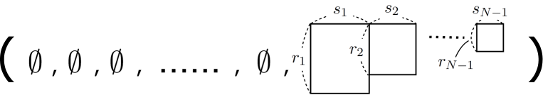
Figure 2: Young diagram corresponding to singular vector. (A)

In fact, Figure 1 means the same Young diagram being on the rightmost side in Figure 2. Hence the projection of this generalized Macdonald function corresponds to the ordinary Macdonald functions associated with the rightmost Young diagram with $N-1$ edges in Figure 2 (Corollary 3.5).

When the condition $r_{k}\geq r_{k+1}$ for the number of screening currents and parameter $\tilde{\alpha}^{(k)}$ in $\left|\chi_{\vec{r},\vec{s}}\right\rangle$ is removed, the above figure is not a Young diagram. However it turns out that the vector $\left|\chi_{\vec{r},\vec{s}}\right\rangle$ coincides with the generalized Macdonald function obtained by cutting off the protruding part and moving boxes to the Young diagrams on the left side. For example, if $0\leq r_{k}<r_{k+1}$ for all $k$, the corresponding $N$-tuple of Young diagrams of the generalized Macdonald function is Figure 3 (Theorem 3.4. (B). (main theorem)).

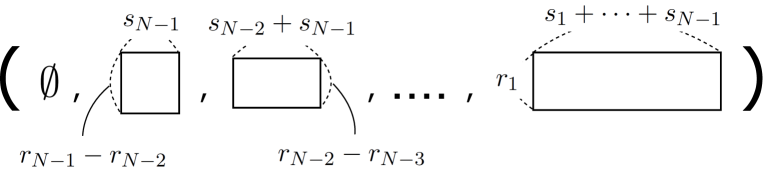
Figure 3: Young diagram corresponding to singular vector. (B)

1.4. Furthermore, we investigate behavior in the limit to the Hall-Littlewood functions, $q\rightarrow 0$, of the deformed Virasoro algebra and the algebra $\mathcal{A}(N)$. Also 5D AGT conjecture is studied in this limit. The reason of considering such a limit is that the situation becomes simple and some problems are solved. In particular, the simplest 5D AGT conjecture can be proved, and PBW type vectors can be expressed in terms of Hall-Littlewood functions. By virtue of the theory of Hall-Littlewood functions, we can obtain and prove an explicit formula (Theorem 4.23) for the four-point correlation function of a certain operator $\tilde{\Phi}^{\vec{v}}_{\vec{u}}(z):\mathcal{F}_{\vec{u}}\rightarrow\mathcal{F}_{\vec{v}}$, which is the limit $q\rightarrow 0$ of the vertex operator $\Phi(z)$ associated with $\mathcal{A}(2)$. Here, $\mathcal{F}_{\vec{u}}$ is the Fock module with the highest weight $\vec{u}=(u_{1},u_{2})$.

Theorem.

$$\left\langle\vec{w}\right|\tilde{\Phi}^{\vec{w}}_{\vec{v}}(z_{2})\tilde{\Phi}^{\vec{v}}_{\vec{u}}(z_{1})\left|\vec{u}\right\rangle=\sum_{\lambda}\left(\frac{u_{1}u_{2}z_{1}}{w_{1}w_{2}z_{2}}\right)^{|\lambda|}\frac{\prod_{k=1}^{\ell(\lambda)}\left(1-t^{k-1}\frac{w_{1}w_{2}}{v_{1}v_{2}}\right)}{t^{2n(\lambda)}b_{\lambda}(t^{-1})}.$$ (1.12)

Here for a partition $\lambda$, $n(\lambda)\mathbin{:=}\sum_{i\geq 1}(i-1)\lambda_{i}$, and $b_{\lambda}$ is the same one in (1.8).

The function $\left\langle\vec{w}\right|\tilde{\Phi}(z_{2})\tilde{\Phi}(z_{1})\left|\vec{u}\right\rangle$ can be calculated by the generalized Hall-Littlewood functions in the same way as [39]. However, we can obtain this formula by inserting the identity with respect to the PBW type vectors.

We call this Hall-Littlewood limit $q\rightarrow 0$ ‘crystallization’ after the use of the quantum groups [50], where the parameter $q$ represents the temperature in the RSOS model [51] which has symmetry of the deformed Virasoro algebra, and the limit $q\rightarrow 0$ can be considered as the zero temperature limit. Although our studies are mathematically different from the notion of the original crystal base of quantum groups, the physical meaning and the motivation to simplify phenomena are the same. To investigate their mathematical relationship is an interesting open problem. On the other hand, little is known about the physical meaning of the Hall-Littlewood limit in the gauge thoery at present.

1.5. In this thesis, the R-matrix of the DIM algebra is also investigated. The result with respect to the R-matrix is based on the collaborative researches [52, 53], and only works of the author is described. In general, a R-matrix is defined as a solution of the Yang-Baxter equation, and is closely related to the solvable lattice models, the knot invariants and so on. Further, it is well-known that R-matrices can be constructed by Hopf algebras such as the quantum groups. In general, a Hopf algebra $H$ with the coproduct $\Delta$ is called quasi-cocommutative if there exists an invertible element $\mathcal{R}$ in the algebra $H\otimes H$ such that

$$\Delta^{\mathrm{op}}(x)=\mathcal{R}\Delta(x)\mathcal{R}^{-1}\quad(\forall x\in H).$$ (1.13)

This $\mathcal{R}$ is called the universal R-matrix. If $\mathcal{R}$ also satisfies the relations

$$(\Delta\otimes\mathrm{id})\mathcal{R}=\mathcal{R}_{13}\mathcal{R}_{23},\quad(\mathrm{id}\otimes\Delta)\mathcal{R}=\mathcal{R}_{13}\mathcal{R}_{12},$$ (1.14)

(see definition of $\mathcal{R}_{ij}$ in Section 5) then $H$ is called quasi-triangular and $\mathcal{R}$ satisfies the Yang-Baxter equation $\mathcal{R}_{12}\mathcal{R}_{13}\mathcal{R}_{23}=\mathcal{R}_{23}\mathcal{R}_{13}\mathcal{R}_{12}$. The DIM algebra is known to be quasi-triangular [42]. In this thesis, the representation matrix of the universal R-matrix $\mathcal{R}$ is explicitly calculated. In the tensor product of the level 1 representation of the DIM algebra (we denote it by $\rho_{u_{1}u_{2}}$), it is block-diagonalized at each level of the free boson Fock space. Also, it can be seen that the action of $\mathcal{R}$ on the generalized Macdonald functions corresponds to the exchange of spectral parameters, partitions, and variables in the generalized Macdonald functions. Moreover, by using the renormalized generalized Macdonald functions (the integral form $\left|K\right\rangle$), it can be conjectured that

$$\rho_{u_{1}u_{2}}(\mathcal{R})|K_{\vec{\lambda}}\rangle=|K^{\mathrm{op}}_{\vec{\lambda}}\rangle,$$ (1.15)

where $\left|K^{\mathrm{op}}\right\rangle$ is the vector obtained by exchanging partitions, variables and spectral parameters in $\left|K_{\vec{\lambda}}\right\rangle$ (see definitions in Section 5.1). As a consequence, we have conjecture (Conjecture 5.1) of the explicit formula for the representation matrix $R_{\vec{\lambda},\vec{\mu}}$ of the universal R-matrix in the basis of $\left|K_{\vec{\lambda}}\right\rangle$:

Conjecture.

$$R_{\vec{\lambda},\vec{\mu}}\overset{?}{=}\frac{1}{\left\langle K_{\vec{\mu}}|K_{\vec{\mu}}\right\rangle}\left\langle K_{\vec{\mu}}|K^{\mathrm{op}}_{\vec{\lambda}}\right\rangle.$$ (1.16)

In [52, 53], the RTT relation of the DIM algebra is also studied using this R-matirx.

1.6. This thesis is organized as follows. In Section 2, two examples of the 5D AGT conjecture are reviewed. One is the correspondence between the Whittaker vector of the deformed Virasoro algebra and the partition function of the 5D pure gauge theory. The other is the conjecture on the AFLT basis using the level $N$ representation of the DIM algebra. In Section 3, we give a factorized formula for the Kac determinant of the algebra $\mathcal{A}(N)$. Its proof depends on some results of the deformed $W$-algebra. The relationship between the singular vectors and the generalized Macdonald functions is also revealed. In Section 4, we investigated the $q\rightarrow 0$ limit of the deformed Virasoro algebra, the algebra $\mathcal{A}(N)$ and the 5D AGT conjecture. In particular, the simplest 5D AGT conjecture is proved in this limit. In Section 5, the explicit form of the representation of the universal R-matrix of the DIM algebra is calculated. Its general form is also conjectured in terms of the generalized Macdonald functions. In Section 6, properties of the generalized Macdonald functions are studied. First, to state the existence theorem of the generalized Macdonald functions, we need partial orderings among $N$-tuples of partitions. In this thesis, by using the partial orderings $\mathop{\overset{*}{>}}$ (see Definition 2.10) and $\mathop{\overset{*}{\succ}}$ (see Definition 6.1), the existence theorem is proved. However, in [39], another ordering $>^{\mathrm{L}}$ is used and the proof of existence theorem [39, Proposition 3.8] is omitted. We justify the theorem [39, Proposition 3.8] by comparing $\mathop{\overset{*}{\succ}}$ and $>^{\mathrm{L}}$ in Subsection 6.1. In Subsection 6.2, we also investigate the action of the generators $X^{(1)}_{\pm 1}$ and higher rank Hamiltonians on the generalized Macdonald functions. Their actions are based on a conversion rule called spectral duality that exchanges the level $N$ representation and the rank $N$ representation of the DIM algebra. Furthermore, in Subsection 6.3, the $q\rightarrow 1$ limit is also studied. Since the generalized Jack functions have degenerate eigenvalues, their Cauchy formula used in the senario of proof of the AGT conjecture [28] is non-trivial. By taking the limit from the Macdonald functions, we can justify the orthogonality of the generalized Jack functions and show the Cauchy formula. In Appendix A, the definition and basic facts of the ordinary Macdonald functions and the Hall-Littlwood functions are briefly reviewed following [5]. In Appendix B, the definition of the DIM algebra and the level $N$ representation are explained following mainly [46, 54, 55]. Moreover we also describe the definition of another representation of the DIM algebra called level $(0,1)$ representation or the rank $N$ representation. In Appendix C, we present some proofs and checks of conjectures in Section 4. At last in Appendix D, we give explicit examples of R-matrix at level 2.

Notations

• $\mathbb{N},\>\mathbb{Z},\>\mathbb{Q},\>\mathbb{R},\>\mathbb{C}$ denote the set of positive integers, integers, rational numbers, real numbers, complex numbers, respectively.

• $\mathbb{Z}_{\geq 0}$ denotes the set of non-negative integers.

• $\mathbb{Z}_{\neq 0}$ denotes the set of integers except $0$.

• $\delta_{i,j}$ denotes the Kronecker delta.

• $\mathbb{K}[x_{1},\ldots,x_{n}]$ denotes the ring of polynomials in $x_{1},\ldots,x_{n}$ over a field $\mathbb{K}$.

• $\#\{\qquad\}$ denotes the cardinality of set.

• Functions $f(a_{1},a_{2},\ldots)$ depending on multiple variables $a_{n}$ ($n=1,2,\ldots$) are occasionally written as $f(a)$ or $f(a_{n})$ for abbreviation.

• For a partition $\lambda$, $p_{\lambda}$ and $m_{\lambda}$ denote the power sum symmetric function and the monomial symmetric function, respectively.

• For $n\in\mathbb{N}$, $e_{n}$ denotes the elementary symmetric function.

Let us explain the notation of partitions and Young diagrams.

A partition $\lambda=(\lambda_{1},\ldots,\lambda_{n})$ is a non-increasing sequence of integers $\lambda_{1}\geq\ldots\geq\lambda_{n}\geq 0$. We write $\left|\lambda\right|\mathbin{:=}\sum_{i}\lambda_{i}$. The length of $\lambda$, denoted by $\ell(\lambda)$, is the number of elements $\lambda_{i}$ with $\lambda_{i}\neq 0$. Partitions are identified if all elements except $0$ are the same. For example, $(3,2)=(3,2,0)$. $m_{i}=m_{i}(\lambda)$ denotes the number of elements that are equal to $i$ in $\lambda$, and we occasionally write partitions as $\lambda=(1^{m_{1}},2^{m_{2}},3^{m_{3}},\ldots)$. For example, $\lambda=(6,6,6,2,2,1)=(6^{3},2^{2},1)$.

The partitions are identified with the Young diagrams, which are the figures written by putting $\lambda_{i}$ boxes on the $i$-th row and aligning the left side. For example, if $\lambda=(6,4,3,3,1)$, its Young diagram is

.

The conjugate of a partition $\lambda$, denoted by $\lambda^{\prime}$, is the partition whose Young diagram is the transpose of the diagram $\lambda$. For example, The conjugate of $\lambda=(6,4,3,3,1)$ is $\lambda^{\prime}=(5,4,4,2,1,1)$. For a partition $\lambda$ and a coordinate $(i,j)\in\mathbb{N}^{2}$, define

$$A_{\lambda}(i,j):=\lambda_{i}-j,\qquad\qquad L_{\lambda}(i,j):=\lambda^{\prime}_{j}-i.$$ (1.17)

$A_{\lambda}(i,j)$ is called arm length and $L_{\lambda}(i,j)$ is called leg length. In the diagram, they mean the numbers of boxes in right side from or below the box being in the $i$-th row and $j$-th column. For example, if $\lambda=(8,8,5,3,3,3,1)$, then $A_{\lambda}(2,3)=5$, $L_{\lambda}(2,3)=4$.

Note that they can take negative values as $A_{\lambda}(3,7)=-2$, $L_{\lambda}(3,7)=-1$. For a partition $\lambda$, we define $n(\lambda):=\sum_{i\geq 1}(i-1)\lambda_{i}$. This means the sum of the numbers obtained by attaching a zero to box in the top row of the Young diagram of $\lambda$, a $1$ to each box in the second row, and so on.

For $N$-tuple of partitions $\vec{\lambda}=(\lambda^{(1)},\ldots,\lambda^{(N)})$, define $|\vec{\lambda}|:=|\lambda^{(1)}|+\cdots+|\lambda^{(N)}|$. If $|\vec{\lambda}|=m$, we occasionally use the symbol ”$\vdash$” as $\vec{\lambda}\vdash m$.

2 5D AGT conjecture

2.1 Review of the simplest 5D AGT correspondence

We start with recapitulating the result of the Whittaker vector of the deformed Virasoro algebra and the simplest five-dimensional AGT correspondence.

Definition 2.1.

Let $q$ and $t$ be independent parameters and $p\mathbin{:=}q/t$. The deformed Virasoro algebra is the associative algebra over $\mathbb{Q}(q,t)$ generated by $T_{n}$ ($n\in\mathbb{Z}$) with the commutation relation

$$[T_{n},T_{m}]=-\sum_{l=1}^{\infty}f_{l}(T_{n-l}T_{m+l}-T_{m-l}T_{n+l})-\frac{(1-q)(1-t^{-1})}{1-p}(p^{n}-p^{-n})\delta_{n+m,0},$$ (2.1)

where the structure constant $f_{l}\in\mathbb{Q}(q,t)$ is defined by

$$f(z)=\sum_{l=0}^{\infty}f_{l}\>z^{l}\mathbin{:=}\exp\left(\sum_{n=1}^{\infty}\frac{1}{n}\frac{(1-q^{n})(1-t^{-n})}{1+p^{n}}z^{n}\right).$$ (2.2)

The relation (2.1) can be written in terms of the generating function $T(z)\mathbin{:=}\sum_{n\in\mathbb{Z}}T_{n}z^{-n}$ as

$$f\left(\frac{w}{z}\right)T(z)T(w)-T(w)T(z)f\left(\frac{z}{w}\right)=-\frac{(1-q)(1-t^{-1})}{1-p}\left[\delta\left(\frac{pw}{z}\right)-\delta\left(\frac{p^{-1}w}{z}\right)\right],$$ (2.3)

where $\delta(x)=\sum_{n\in\mathbb{Z}}x^{n}$.

The deformed Virasoro algebra is introduced in [14]. Let $\left|h\right\rangle$ be the highest weight vector such that $T_{0}\left|h\right\rangle=h\left|h\right\rangle$, $T_{n}\left|h\right\rangle=0$ ($n>0$), and $M_{h}$ be the Verma module generated by $\left|h\right\rangle$. Similarly, $\left\langle h\right|$ is the vector satisfying the condition that $\left\langle h\right|T_{0}=h\left\langle h\right|$, $\left\langle h\right|T_{n}=0$ ($n<0$). $M^{*}_{h}$ is the dual module generated by $\left\langle h\right|$. The PBW type vectors $|T_{-\lambda}\rangle\mathbin{:=}T_{-\lambda_{1}}T_{-\lambda_{2}}\cdots\left|h\right\rangle$ for partitions $\lambda$ form a basis over $M_{h}$. Also, $\left\langle T_{\lambda}\right|\mathbin{:=}\left\langle h\right|\cdots T_{\lambda_{2}}T_{\lambda_{1}}$ form a basis over $M^{*}_{h}$. Here $\lambda=(\lambda_{1},\lambda_{2},\ldots)$ is a partition or a Young diagram. The bilinear form $M^{*}_{h}\otimes M_{h}\rightarrow\mathbb{C}$ is uniquely defined by $\left\langle h|h\right\rangle=1$. This bilinear form is called the Shapovalov form. The Whittaker vector $\left|G\right\rangle$ is defined as follows.

Definition 2.2 ([36]).

For a generic parameter $\Lambda$, define the Whittaker vector $\left|G\right\rangle$ by the relations

$$T_{1}\left|G\right\rangle=\Lambda^{2}\left|G\right\rangle,\qquad T_{n}\left|G\right\rangle=0\quad(n>1).$$ (2.4)

Similarly, the dual Whittaker vector $\left\langle G\right|\in M_{h}^{*}$ is defined by the condition that

$$\left\langle G\right|T_{-1}=\Lambda^{2}\left\langle G\right|,\qquad\left\langle G\right|T_{n}=0\quad(n<-1).$$ (2.5)

This vector is in the form $\left|G\right\rangle=\sum_{\lambda}\Lambda^{2|\lambda|}B^{\lambda,(1^{n})}T_{-\lambda}\left|h\right\rangle$ and its norm is calculated as $\left\langle G|G\right\rangle=\sum_{n=0}^{\infty}\Lambda^{4n}B^{(1^{n}),(1^{n})}$, where $B^{\lambda,\mu}$ denotes the inverse matrix element of the Shapovalov matrix $B_{\lambda,\mu}:=\left\langle T_{\lambda}|T_{-\mu}\right\rangle$.

It is useful to consider the free field representation of the deformed Virasoro algebra. By the Heisenberg algebra generated by $a_{n}$ ($n\in\mathbb{Z}$) and $Q$ with the relations

$$[a_{n},a_{m}]=n\frac{1-q^{|n|}}{1-t^{|n|}}\delta_{n+m,0},\qquad[a_{n},Q]=\delta_{n,0},$$ (2.6)

the generating function $T(z)$ can be represented as

$$T(z) =\Lambda^{+}(z)+\Lambda^{-}(z),$$ (2.7)

$$\Lambda^{\pm}(z) :=\exp\left\{\mp\sum_{n=1}^{\infty}\frac{1-t^{n}}{n(t^{n}+q^{n})}(q/t)^{\mp\frac{n}{2}}a_{-n}z^{n}\right\}\exp\left\{\mp\sum_{n=1}^{\infty}\frac{1-t^{n}}{n}(q/t)^{\pm\frac{n}{2}}a_{n}z^{-n}\right\}K^{\pm}.$$ (2.8)

Here $K^{\pm}\mathbin{:=}e^{\pm a_{0}}$. Let $\left|0\right\rangle$ be the highest weight vector in the Fock module of the Heisenberg algebra such that $a_{n}\left|0\right\rangle=0$ ($n\geq 0$), and $\left|k\right\rangle\mathbin{:=}k^{Q}\left|0\right\rangle$. Then $K\left|k\right\rangle=k\left|k\right\rangle$. Furthermore, $\left|k\right\rangle$ can be regarded as the highest weight vector $\left|h\right\rangle$ of the deformed Virasoro algebra with highest weight $h=k+k^{-1}$. In [36], Awata and Yamada conjectured an explicit formula for $\left|G\right\rangle$ in terms of Macdonald functions under the free field representation, and Yanagida proved it in [56]. The simplest five-dimensional AGT conjecture is that the inner product $\left\langle G|G\right\rangle$ coincides with the five-dimensional (K-theoretic) Nekrasov formula for pure $SU(2)$ gauge theory [47, 57, 58] :

$$Z^{\mathrm{inst}}_{\mathrm{pure}} \mathbin{:=}\sum_{\lambda,\mu}\frac{(\Lambda^{4}t/q)^{|\lambda|+|\mu|}}{N_{\lambda\lambda}(1)N_{\lambda\mu}(Q)N_{\mu\mu}(1)N_{\mu\lambda}(Q^{-1})},$$ (2.9)

$$N_{\lambda\mu}(Q) \mathbin{:=}\prod_{(i,j)\in\lambda}\left(1-Qq^{A_{\lambda}(i,j)}t^{L_{\mu}(i,j)+1}\right)\prod_{(i,j)\in\mu}\left(1-Qq^{-A_{\mu}(i,j)-1}t^{-L_{\lambda}(i,j)}\right),$$ (2.10)

where $A_{\lambda}(i,j)$ and $L_{\lambda}(i,j)$ are the arm length and the leg length defined in Introduction, and $\lambda^{\prime}$ is the conjugate of $\lambda$.

Fact 2.3.

For $k=Q^{\frac{1}{2}}$,

$$\left\langle G|G\right\rangle=Z^{\mathrm{inst}}_{\mathrm{pure}}.$$ (2.11)

This fact is conjectured in [36] and proved in [59, 60] when the parameter $q$ is generic.

2.2 Reargument of Ding-Iohara-Miki algebra and AGT correspondence

We now turn to the DIM algebra [61, 40]. Let us recall the AFLT basis in the 5D AGT correspondence of the $SU(N)$ gauge theory along [39]. In this section, we use $N$ kinds of bosons $a_{n}^{(i)}$ ($n\in\mathbb{Z}_{\neq 0}$, $i=1,2,\ldots,N$) and $U_{i}$ with the relations

$$[a^{(i)}_{n},a^{(j)}_{m}]=n\frac{1-q^{|n|}}{1-t^{|n|}}\,\delta_{i,j}\,\delta_{n+m,0},$$ (2.12)

$$[a^{(i)}_{n},U_{j}]=0,\quad[U_{i},U_{j}]=0,\qquad(\forall i,j,n).$$ (2.13)

Here $U_{i}$ is the substitution of zero mode $a^{(i)}_{0}$, which is realized in two different ways in Sections 3 and 4, respectively. Let us define the vertex operators $\eta^{(i)}$ and $\varphi^{(i)}$.

Definition 2.4.

Set

$$\eta^{(i)}(z) :=\exp\left(\sum_{n=1}^{\infty}\frac{1-t^{-n}}{n}\,z^{n}a^{(i)}_{-n}\right)\exp\left(-\sum_{n=1}^{\infty}\frac{(1-t^{n})}{n}\,z^{-n}a^{(i)}_{n}\right),$$ (2.14)

$$\varphi^{(i)}(z) :=\exp\left(\sum_{n=1}^{\infty}\frac{1-t^{-n}}{n}(1-p^{-n})z^{n}a^{(i)}_{-n}\right).$$ (2.15)

Definition 2.5.

Define generators $X^{(i)}(z)=\sum_{n}X^{(i)}_{n}z^{-n}$ by

$$X^{(i)}(z) \mathbin{:=}\sum_{1\leq j_{1}<\cdots<j_{i}\leq N}{\hbox to0.0pt{\raise 1.72218pt\hbox{$\scriptscriptstyle\bullet$}\hss}\lower 1.72218pt\hbox{$\scriptscriptstyle\bullet$}}\Lambda_{j_{1}}(z)\cdots\Lambda_{j_{i}}(p^{i-1}z){\hbox to0.0pt{\raise 1.72218pt\hbox{$\scriptscriptstyle\bullet$}\hss}\lower 1.72218pt\hbox{$\scriptscriptstyle\bullet$}},$$ (2.16)

where $\scriptscriptstyle\bullet$$\scriptscriptstyle\bullet$   $\scriptscriptstyle\bullet$$\scriptscriptstyle\bullet$ denotes the usual normal ordered product, and

$$\Lambda^{i}(z):=\varphi^{(1)}(z)\varphi^{(2)}(zp^{-\frac{1}{2}})\cdots\varphi^{(i-1)}(zp^{-\frac{i-2}{2}})\eta^{(i)}(zp^{-\frac{i-1}{2}})U_{i}.$$ (2.17)

The generator $X^{(1)}(z)$ arises from the level $N$ representation of Ding-Iohara-Miki algebra [46, 41], and is obtained by acting the coproduct of the DIM algebra to the vertex operator $\eta(z)$ $N$ times (see Appendix B). The other generators $X^{(i)}_{n}$ appear in the commutation relations of generators $X^{(i-k)}_{n}$ ($k=1,\ldots i-1$). When we just consider the AGT conjecture, it suffices to deal with the subalgebra $\langle X^{(i)}_{n}\rangle$ in some completion of the endomorphism of the algebra of $N$-tensored Fock modules for our Heisenberg algebra.

Notation 2.6.

We denote the algebra $\langle X^{(i)}_{n}\rangle$ by $\mathcal{A}(N)$.

Proposition 2.7.

If $N=2$, the commutation relations of the generators are

$$f^{(1)}\left(\frac{w}{z}\right)X^{(1)}(z)X^{(1)}(w)-X^{(1)}(w)X^{(1)}(z)f^{(1)}\left(\frac{z}{w}\right)$$ (2.18)

$$\qquad\qquad\qquad=\frac{(1-q)(1-t^{-1})}{1-p}\left\{\delta\left(\frac{w}{pz}\right)X^{(2)}(z)-\delta\left(\frac{pw}{z}\right)X^{(2)}(w)\right\},$$

$$f^{(2)}\left(\frac{w}{z}\right)X^{(2)}(z)X^{(2)}(w)-X^{(2)}(w)X^{(2)}(z)f^{(2)}\left(\frac{z}{w}\right)=0,$$ (2.19)

$$f^{(1)}\left(\frac{pw}{z}\right)X^{(1)}(z)X^{(2)}(w)-X^{(2)}(w)X^{(1)}(z)f^{(1)}\left(\frac{z}{w}\right)=0,$$ (2.20)

where $\delta(x)=\sum_{n\in\mathbb{Z}}x^{n}$ is the multiplicative delta function and the structure constant $f^{(i)}(z)=\sum_{l=0}^{\infty}f^{(i)}_{l}z^{l}$ is defined by

$$f^{(1)}(z)\mathbin{:=}\exp\left\{\sum_{n>0}\frac{(1-q^{n})(1-t^{-n})}{n}z^{n}\right\},$$ (2.21)

$$f^{(2)}(z)\mathbin{:=}\exp\left\{\sum_{n>0}\frac{(1-q^{n})(1-t^{-n})(1+p^{n})}{n}z^{n}\right\}.$$ (2.22)

These relations are equivalent to

$$[X^{(1)}_{n},X^{(1)}_{m}]=-\sum_{l=1}^{\infty}f^{(1)}_{l}(X^{(1)}_{n-l}X^{(1)}_{m+l}-X^{(1)}_{m-l}X^{(1)}_{n+l})+\frac{(1-q)(1-t^{-1})}{1-p}(p^{m}-p^{n})X^{(2)}_{n+m},$$ (2.23)

$$[X^{(2)}_{n},X^{(2)}_{m}]=-\sum_{l=1}^{\infty}f^{(2)}_{l}(X^{(2)}_{n-l}X^{(2)}_{m+l}-X^{(2)}_{m-l}X^{(2)}_{n+l}),$$ (2.24)

$$[X^{(1)}_{n},X^{(2)}_{m}]=-\sum_{l=1}^{\infty}f^{(1)}_{l}(p^{l}X^{(1)}_{n-l}X^{(2)}_{m+l}-X^{(2)}_{m-l}X^{(1)}_{n+l}).$$ (2.25)

The proof is similar to the calculation of the deformed Virasoro algebra or the deformed $W$-algebra. In the formula (2.18), we use

$$f^{(1)}(x)-f^{(1)}(1/px)=\frac{(1-q)(1-t^{-1})}{1-p}\left(\delta(x)-\delta(px)\right).$$ (2.26)

For an $N$-tuple of parameters $\vec{u}=(u_{1},\ldots,u_{N})$, define $\left|\vec{u}\right\rangle$ and $\left\langle\vec{u}\right|$ to be the highest weight vectors such that $a_{n}^{(i)}\left|\vec{u}\right\rangle=\left\langle\vec{u}\right|a^{(i)}_{-n}=0$ ($n\geq 1$, $\forall i$), $U_{i}\left|\vec{u}\right\rangle=u_{i}\left|\vec{u}\right\rangle$ and $\left\langle\vec{u}\right|U_{i}=u_{i}\left\langle\vec{u}\right|$. $\mathcal{F}_{\vec{u}}$ is the highest weight module generated by $\left|\vec{u}\right\rangle$, and $\mathcal{F}_{\vec{u}}^{*}$ is the dual module generated by $\left\langle\vec{u}\right|$. The bilinear form (Shapovalov form) $\mathcal{F}_{\vec{u}}^{*}\otimes\mathcal{F}_{\vec{u}}\rightarrow\mathbb{C}$ is uniquely determined by the condition $\left\langle\vec{u}|\vec{u}\right\rangle$.

Definition 2.8.

For an $N$-tuple of partitions $\vec{\lambda}=(\lambda^{(1)},\lambda^{(2)},\ldots,\lambda^{(N)})$, set

$$\left|X_{\vec{\lambda}}\right\rangle\mathbin{:=}X^{(1)}_{-\lambda^{(1)}_{1}}X^{(1)}_{-\lambda^{(1)}_{2}}\cdots X^{(2)}_{-\lambda^{(2)}_{1}}X^{(2)}_{-\lambda^{(2)}_{2}}\cdots X^{(N)}_{-\lambda^{(N)}_{1}}X^{(N)}_{-\lambda^{(N)}_{2}}\cdots\left|\vec{u}\right\rangle,$$ (2.27)

$$\left\langle X_{\vec{\lambda}}\right|\mathbin{:=}\left\langle\vec{u}\right|\cdots X^{(N)}_{\lambda^{(N)}_{2}}X^{(N)}_{\lambda^{(N)}_{1}}\cdots X^{(2)}_{\lambda^{(2)}_{2}}X^{(2)}_{\lambda^{(2)}_{1}}\cdots X^{(1)}_{\lambda^{(1)}_{2}}X^{(1)}_{\lambda^{(1)}_{1}}.$$ (2.28)

The PBW theorem cannot be used because the algebra $\mathcal{A}(N)$ is not a Lie algebra, but in [39] it was conjectured that the PBW type vectors $\left|X_{\vec{\lambda}}\right\rangle$ and $\left\langle X_{\vec{\lambda}}\right|$ are a basis over $\mathcal{F}_{\vec{u}}$ and $\mathcal{F}_{\vec{u}}^{*}$, respectively. This conjecture can be solved by the Kac determinant of the algebra $\mathcal{A}(N)$, which is proved in Section 3. In this section, we consider another type of the PBW basis, since it has good expression in $q\rightarrow 0$ limit in terms of the Hall-Littlewood functions (see Section 4.3).

Definition 2.9.

For $\vec{\lambda}=(\lambda^{(1)},\lambda^{(2)},\ldots,\lambda^{(N)})$, set

$$|X^{\prime}_{\vec{\lambda}}\rangle\mathbin{:=}X^{(N)}_{-\lambda^{(N)}_{1}}X^{(N)}_{-\lambda^{(N)}_{2}}\cdots X^{(2)}_{-\lambda^{(2)}_{1}}X^{(2)}_{-\lambda^{(2)}_{2}}\cdots X^{(1)}_{-\lambda^{(1)}_{1}}X^{(1)}_{-\lambda^{(1)}_{2}}\cdots\left|\vec{u}\right\rangle,$$ (2.29)

$$\langle X^{\prime}_{\vec{\lambda}}|\mathbin{:=}\left\langle\vec{u}\right|\cdots X^{(1)}_{\lambda^{(1)}_{2}}X^{(1)}_{\lambda^{(1)}_{1}}\cdots X^{(2)}_{\lambda^{(2)}_{2}}X^{(2)}_{\lambda^{(2)}_{1}}\cdots X^{(N)}_{\lambda^{(N)}_{2}}X^{(N)}_{\lambda^{(N)}_{1}}.$$ (2.30)

Let us review the AFLT basis in $\mathcal{F}_{\vec{u}}$, which is also called generalized Macdonald functions. In order to state its existence theorem, let us prepare the following ordering.

Definition 2.10.

For $N$-tuple of partitions $\vec{\lambda}$ and $\vec{\mu}$,

$$\vec{\lambda}\mathop{\overset{*}{>}}\vec{\mu}\quad\overset{\mathrm{def}}{\Longleftrightarrow}\quad |\vec{\lambda}|=|\vec{\mu}|,\quad\sum_{i=k}^{N}|\lambda^{(i)}|\geq\sum_{i=k}^{N}|\mu^{(i)}|\quad(\forall k)\quad\mathrm{and}$$ (2.31)

$$(|\lambda^{(1)}|,|\lambda^{(2)}|,\ldots,|\lambda^{(N)}|)\neq(|\mu^{(1)}|,|\mu^{(2)}|,\ldots,|\mu^{(N)}|).$$

Here $|\vec{\lambda}|\mathbin{:=}|\lambda^{(1)}|+\cdots+|\lambda^{(N)}|$. Note that the second condition can be replaced with $\sum_{i=1}^{k-1}|\lambda^{(i)}|\leq\sum_{i=1}^{k-1}|\mu^{(i)}|\quad(\forall k)$.

We can state the existence theorem of generalized Macdonald functions in the basis of products of Macdonald functions $\prod_{i=1}^{N}P_{\lambda^{(i)}}(a^{(i)}_{-n};q,t)\left|\vec{u}\right\rangle$, where $P_{\lambda}(a_{-n}^{(i)};q,t)$ are Macdonald symmetric functions defined in Appendix A with substituting the bosons $a^{(i)}_{-n}$ for the power sum symmetric functions $p_{n}$.

Proposition 2.11.

For each $N$-tuple of partitions $\vec{\lambda}$, there exists a unique vector $\left|P_{\vec{\lambda}}\right\rangle\in\mathcal{F}_{\vec{u}}$ such that

$$\left|P_{\vec{\lambda}}\right\rangle=\prod_{i=1}^{N}P_{\lambda^{(i)}}(a^{(i)}_{-n};q,t)\left|\vec{u}\right\rangle+\sum_{\vec{\mu}\mathop{\overset{*}{<}}\vec{\lambda}}c_{\vec{\lambda},\vec{\mu}}\prod_{i=1}^{N}P_{\mu^{(i)}}(a^{(i)}_{-n};q,t)\left|\vec{u}\right\rangle,$$ (2.32)

$$X^{(1)}_{0}\left|P_{\vec{\lambda}}\right\rangle=\epsilon_{\vec{\lambda}}\left|P_{\vec{\lambda}}\right\rangle,$$ (2.33)

where $c_{\vec{\lambda},\vec{\mu}}=c_{\vec{\lambda},\vec{\mu}}(u_{1},\ldots,u_{N};q,t)$ is a constant, $\epsilon_{\vec{\lambda}}=\epsilon_{\vec{\lambda}}(u_{1},\ldots,u_{N};q,t)$ is the eigenvalue of $X^{(1)}_{0}$. Similarly, there exists a unique vector $\left\langle P_{\vec{\lambda}}\right|\in\mathcal{F}_{\vec{u}}^{*}$ such that

$$\left\langle P_{\vec{\lambda}}\right|=\left\langle\vec{u}\right|\prod_{i=1}^{N}P_{\lambda^{(i)}}(a^{(i)}_{n};q,t)+\sum_{\vec{\mu}\mathop{\overset{*}{>}}\vec{\lambda}}c_{\vec{\lambda},\vec{\mu}}^{*}\left\langle\vec{u}\right|\prod_{i=1}^{N}P_{\mu^{(i)}}(a^{(i)}_{n};q,t),$$ (2.34)

$$\left\langle P_{\vec{\lambda}}\right|X^{(1)}_{0}=\epsilon_{\vec{\lambda}}^{*}\left\langle P_{\vec{\lambda}}\right|.$$ (2.35)

Then the eigenvalues are

$$\epsilon_{\vec{\lambda}}=\epsilon_{\vec{\lambda}}^{*}=\sum_{k=1}^{N}u_{k}e_{\lambda^{(k)}},\quad e_{\lambda}:=1+(t-1)\sum_{i\leq 1}(q^{\lambda_{i}}-1)t^{-i}.$$ (2.36)

Although the ordering of Definition 2.10 is different from the one in [39], the eigenfunctions $\left|P_{\vec{\lambda}}\right\rangle$ are quite the same. The proof is similar to the one in Section 6.1, which follows from triangulation of $X^{(1)}_{0}$. By this proposition, it can be seen that $\left|P_{\vec{\lambda}}\right\rangle$ is a basis over $\mathcal{F}_{\vec{u}}$, and the eigenvalues of $X^{(1)}_{0}$ are non-degenerate. In Section 6.1, a more elaborated ordering is introduced and a relationship between these orderings is explained. In Section 6.3, it is shown that these vectors $\left|P_{\vec{\lambda}}\right\rangle$ correspond to the generalized Jack functions defined in [28] in the $q\rightarrow 1$ limit. To use generalized Macdonald functions in the AGT correspondence, we need to consider its integral form. In this paper, we adopt the following renormalization, which is slightly different from that of [39].

Definition 2.12.

Define the vectors $\left|K_{\vec{\lambda}}\right\rangle$ and $\left\langle K_{\vec{\lambda}}\right|$, called the integral forms, by the condition that

$$\left|K_{\vec{\lambda}}\right\rangle=\sum_{\vec{\mu}}\alpha_{\vec{\lambda}\vec{\mu}}\left|X^{\prime}_{\vec{\mu}}\right\rangle\propto\left|P_{\vec{\lambda}}\right\rangle,\quad\alpha_{\vec{\lambda},(\emptyset,\ldots,\emptyset,(1^{|\vec{\lambda}|}))}=1,$$ (2.37)

$$\left\langle K_{\vec{\lambda}}\right|=\sum_{\vec{\mu}}\beta_{\vec{\lambda}\vec{\mu}}\left\langle X^{\prime}_{\vec{\mu}}\right|\propto\left\langle P_{\vec{\lambda}}\right|,\quad\beta_{\vec{\lambda},(\emptyset,\ldots,\emptyset,(1^{|\vec{\lambda}|}))}=1.$$ (2.38)

Conjecture 2.13.

The coefficients $\alpha_{\vec{\lambda}\vec{\mu}}$ and $\beta_{\vec{\lambda}\vec{\mu}}$ are polynomials in $q^{\pm 1}$, $t^{\pm 1}$ and $u_{i}$ with integer coefficients.

Example 2.14.

If $N=2$, the transition matrix $\alpha_{\vec{\lambda},\vec{\mu}}$ is as follows:

$$\begin{array}[]{c||c c}\vec{\lambda}\setminus\vec{\mu}&(\emptyset,(1))&((1),\emptyset)\\ \hline\cr\hline\cr(\emptyset,(1))&1&-\frac{qu_{2}}{t}\\ ((1),\emptyset)&1&-\frac{qu_{1}}{t}\end{array},$$

$$\begin{array}[]{c||c c c }\vec{\lambda}\setminus\vec{\mu}&(\emptyset,(2))&(\emptyset,(1^{2}))&((1),(1))\\ \hline\cr\hline\cr(\emptyset,(2))&\frac{(q-1)u_{2}\left(tu_{1}q^{2}-u_{1}q^{2}+tu_{2}q^{2}-u_{2}q^{2}-u_{2}q+tu_{1}\right)}{t^{2}}&1&-\frac{q(q+1)u_{2}}{t}\\ (\emptyset,(1^{2}))&\frac{q(t-1)u_{2}\left(-u_{1}t^{2}+qu_{2}t+qu_{1}-u_{1}+qu_{2}-u_{2}\right)}{t^{3}}&1&-\frac{q(t+1)u_{2}}{t^{2}}\\ ((1),(1))&\frac{(q-1)q(t-1)\left(u_{1}^{2}+u_{2}u_{1}+u_{2}^{2}\right)}{t^{2}}&1&-\frac{q(u_{1}+u_{2})}{t}\\ ((2),\emptyset)&\frac{(q-1)u_{1}\left(tu_{1}q^{2}-u_{1}q^{2}+tu_{2}q^{2}-u_{2}q^{2}-u_{1}q+tu_{2}\right)}{t^{2}}&1&-\frac{q(q+1)u_{1}}{t}\\ ((1^{2}),\emptyset)&\frac{q(t-1)u_{1}\left(-u_{2}t^{2}+qu_{1}t+qu_{1}-u_{1}+qu_{2}-u_{2}\right)}{t^{3}}&1&-\frac{q(t+1)u_{1}}{t^{2}}\end{array},$$

$$\begin{array}[]{c|| c c}\vec{\lambda}\setminus\vec{\mu}&((2),\emptyset)&((1^{2}),\emptyset)\\ \hline\cr\hline\cr(\emptyset,(2))&-\frac{(q-1)q^{2}u_{2}^{2}(-qu_{1}+qtu_{1}+tu_{1}-qu_{2})}{t^{3}}&\frac{q^{3}u_{2}^{2}}{t^{2}}\\ (\emptyset,(1^{2}))&-\frac{q^{2}(t-1)u_{2}^{2}(qu_{1}-tu_{1}-u_{1}+qu_{2})}{t^{4}}&\frac{q^{2}u_{2}^{2}}{t^{3}}\\ ((1),(1))&-\frac{(q-1)q^{2}(t-1)u_{1}u_{2}(u_{1}+u_{2})}{t^{3}}&\frac{q^{2}u_{1}u_{2}}{t^{2}}\\ ((2),\emptyset)&-\frac{(q-1)q^{2}u_{1}^{2}(-qu_{1}-qu_{2}+qtu_{2}+tu_{2})}{t^{3}}&\frac{q^{3}u_{1}^{2}}{t^{2}}\\ ((1^{2}),\emptyset)&-\frac{q^{2}(t-1)u_{1}^{2}(qu_{1}+qu_{2}-tu_{2}-u_{2})}{t^{4}}&\frac{q^{2}u_{1}^{2}}{t^{3}}\end{array}.$$

By using these integral forms, the five dimensional AGT conjecture can be stated in the following form. (c.f. [39, Conjecture 3.11 and Conjecture 3.13])

Conjecture 2.15.

The norm of $\left|K_{\vec{\lambda}}\right\rangle$ reproduces the Nekrasov factor:

$$\langle K_{\vec{\lambda}}|K_{\vec{\lambda}}\rangle\overset{?}{=}(-1)^{N}\,e_{N}(\vec{u})^{|\vec{\lambda}|}\,\prod_{i=1}^{N}t^{-Nn(\lambda^{(i)})}q^{Nn(\lambda^{(i)^{\prime}})}u_{i}^{N|\lambda^{(i)}|}\prod_{i,j=1}^{N}N_{\lambda^{(i)},\lambda^{(j)}}(qu_{i}/tu_{j}),$$ (2.39)

where $e_{N}(\vec{u})=u_{1}u_{2}\cdots u_{N}$.

Definition 2.16.

Call the linear operator $\Phi(z)=\Phi^{\vec{v}}_{\vec{u}}(z):\mathcal{F}_{\vec{u}}\rightarrow\mathcal{F}_{\vec{v}}$ the vertex operator if it satisfies

$$(1-e_{N}(\vec{v})w/z)X^{(i)}(z)\Phi(w)=(1-p^{-i}e_{N}(\vec{v})w/z)\Phi(w)X^{(i)}(z)$$ (2.40)

and $\left\langle\vec{v}\right|\Phi(w)\left|\vec{u}\right\rangle=1$. Then the relations for the Fourier components are

$$(X^{(i)}_{n}-e_{N}(\vec{v})wX^{(i)}_{n-1})\Phi(w)=\Phi(w)(X^{(i)}_{n}-(t/q)^{i}e_{N}(\vec{v})wX^{(i)}_{n-1})$$ (2.41)

for $i=1,2,\ldots,N$.

Example 2.17.

If $N=1$, it is known that $\Phi(z)$ exists and is given by

$$\Phi(z)=\exp\left\{-\sum_{n=1}^{\infty}\frac{1}{n}\frac{v^{n}-(t/q)^{n}u^{n}}{1-q^{n}}a_{-n}z^{n}\right\}\exp\left\{\sum_{n=1}^{\infty}\frac{1}{n}\frac{v^{-n}-u^{-n}}{1-q^{-n}}a_{n}z^{-n}\right\}\mathcal{Q},$$ (2.42)

where $\mathcal{Q}$ is the operator from $\mathcal{F}_{u}$ to $\mathcal{F}_{v}$ satisfying the relation $U\mathcal{Q}=(v/u)\,\mathcal{Q}\,U$.

Conjecture 2.18.

The matrix elements of $\Phi(w)$ with respect to generalized Macdonald functions are

$$\left\langle K_{\vec{\lambda}}\right|\Phi^{\vec{v}}_{\vec{u}}(w)\left|K_{\vec{\mu}}\right\rangle \overset{?}{=}(-1)^{|\vec{\lambda}|+(N-1)|\vec{\mu}|}(t/q)^{N(|\vec{\lambda}|-|\vec{\mu}|)}e_{N}(\vec{u})^{|\vec{\lambda}|}e_{N}(\vec{v})^{|\vec{\lambda}|-|\vec{\mu}|}w^{|\vec{\lambda}|-|\vec{\mu}|}$$ (2.43)

$$\quad\times\prod_{i=1}^{N}u_{i}^{N|\mu^{(i)}|}q^{N\,n(\mu^{(i)^{\prime}})}t^{-N\,n(\mu^{(i)})}\times\prod_{i,j=1}^{N}N_{\lambda^{(i)},\mu^{(j)}}(qv_{i}/tu_{j}).$$

Under these conjectures, we can obtain a formula for multi-point correlation functions of $\Phi(z)$ by inserting the identity $1=\sum_{\vec{\lambda}}\frac{\left|K_{\vec{\lambda}}\right\rangle\left\langle K_{\vec{\lambda}}\right|}{\left\langle K_{\vec{\lambda}}|K_{\vec{\lambda}}\right\rangle}$. In particular, the formula for the four-point functions agrees with the 5D $U(N)$ Nekrsov formula with $N_{f}=2N$ matters. An M-theoretic derivation of this formula is also given by [62].

3 Kac determinant and singular vecter of the algebra $\mathcal{A}(N)$

3.1 Kac determinant of the algebra $\mathcal{A}(N)$

In this section, we give the formula for the Kac determinant of the algebra $\mathcal{A}(N)$ and prove it. Moreover, it is shown that singular vectors correspond to the generalized Macdonald functions. In order to prove the Kac determinant, we need screening currents of the algebra $\mathcal{A}(N)$. To construct them, it is necessary to realize the operator $U_{i}$ and the highest wight vector $\left|\vec{u}\right\rangle$ in terms of the charge operator $Q^{(i)}$ and $a^{(i)}_{0}$ ($i=1,\ldots N$). Let $Q^{(i)}$ be the operator satisfying the relation

$$[a^{(i)}_{n},Q^{(j)}]=\delta_{n,0}\delta_{i,j},$$ (3.1)

$\left|0\right\rangle$ be the highest weight vector in the Fock module of the Heisenberg algebra such that $a^{(i)}_{n}\left|0\right\rangle=0$ for $n\geq 0$. For an $N$-tuple of complex parameters $\vec{u}=(u_{1},\ldots,u_{N})$ with $u_{i}=q^{\sqrt{\beta}w_{i}}p^{-\frac{N+1}{2}+i}$, we realize the highest wight vector $\left|\vec{u}\right\rangle$ and $U_{i}$ as

$$U_{i}=q^{\sqrt{\beta}a^{(i)}_{0}}p^{-\frac{N+1}{2}+i},\qquad\left|\vec{u}\right\rangle=e^{\sum_{i=1}^{N}w_{i}Q^{(i)}}\left|0\right\rangle,$$ (3.2)

where $\beta$ is defined by $t=q^{\beta}$. Then they satisfy the required relation $U_{i}\left|\vec{u}\right\rangle=u_{i}\left|\vec{u}\right\rangle$. Similarly, let $\left\langle 0\right|$ be the dual highest weight vector, and $\left\langle\vec{u}\right|=\left\langle 0\right|e^{-\sum_{i=1}^{N}w_{i}Q^{(i)}}$. These highest wight vectors are normalized by $\left\langle 0|0\right\rangle=1$, and satisfy the condition of the Shapovalov form $\left\langle\vec{u}|\vec{u}\right\rangle=1$.

We obtain the formula for the Kac determinant with respect to the PBW type vectors $\left|X_{\vec{\lambda}}\right\rangle$.

Theorem 3.1.

Let $\mathrm{det}_{n}\mathbin{:=}\det\left(\left\langle X_{\vec{\lambda}}|X_{\vec{\mu}}\right\rangle\right)_{\vec{\lambda},\vec{\mu}\vdash n}$. Then

$$\mathrm{det}_{n}= \prod_{\vec{\lambda}\vdash n}\prod_{k=1}^{N}b_{\lambda^{(k)}}(q)b^{\prime}_{\lambda^{(k)}}(t^{-1})$$ (3.3)

$$\times\prod_{\begin{subarray}{c}1\leq r,s\\ rs\leq n\end{subarray}}\left((u_{1}u_{2}\cdots u_{N})^{2}\prod_{1\leq i<j\leq N}(u_{i}-q^{s}t^{-r}u_{j})(u_{i}-q^{-r}t^{s}u_{j})\right)^{P^{(N)}(n-rs)},$$ (3.4)

where $b_{\lambda}(q)\mathbin{:=}\prod_{i\geq 1}\prod_{k=1}^{m_{i}}(1-q^{k})$, $b^{\prime}_{\lambda}(q)\mathbin{:=}\prod_{i\geq 1}\prod_{k=1}^{m_{i}}(-1+q^{k})$, and $m_{i}$ is the number of entries in $\lambda$ equal to $i$. $P^{(N)}(n)$ denotes the number of $N$-tuples of Young diagrams of size $n$, i.e., $\#\big{\{}\vec{\lambda}=(\lambda^{(1)},\ldots,\lambda^{(N)})\big{|}\vec{\lambda}\vdash n\big{\}}$. In particular, if $N=1$,

$$\mathrm{det}_{n}=\prod_{\lambda\vdash n}b_{\lambda}(q)b^{\prime}_{\lambda}(t^{-1})\times u_{1}^{2\sum_{\lambda\vdash n}\ell(\lambda)}.$$ (3.5)

Corollary 3.2.

If $u_{i}\neq 0$ and $u_{i}\neq q^{r}t^{-s}u_{j}$ for any numbers $i$, $j$ and integers $r$, $s$, then the PBW type vectors $\left|X_{\vec{\lambda}}\right\rangle$ (resp. $\left\langle X_{\vec{\lambda}}\right|$) are a basis over $\mathcal{F}_{\vec{u}}$ (resp. $\mathcal{F}^{*}_{\vec{u}}$).

It can be seen that the representation of the algebra $\mathcal{A}(N)$ on the Fock Module $\mathcal{F}_{\vec{u}}$ is irreducible if and only if the parameters $\vec{u}$ satisfy the condition that $u_{i}\neq 0$ and $u_{i}\neq q^{r}t^{-s}u_{j}$. The proof of Theorem 3.1 is given in the next section.

3.2 Proof of Theorem 3.1

It is known that the level $N$ representation of the DIM algebra introduced in the last section can be regarded as the tensor product of the deformed $W_{N}$-algebra and the Heisenberg algebra associated with the $U(1)$ factor [41]. This fact is obtained by a linear transformation of bosons. The point of proof of Theorem 3.1 is to construct singular vectors by using screening currents of the deformed $W_{N}$-algebra under the decomposition of the generators $X^{(i)}(z)$ into the deformed $W_{N}$-algebra part and the $U(1)$ part. In general, a vector $\left|\chi\right\rangle$ in the Fock module $\mathcal{F}_{\vec{u}}$ is called the singular vector of the algebra $\mathcal{A}(N)$ if it satisfies

$$X^{(i)}_{n}\left|\chi\right\rangle=0$$ (3.6)

for all $i$ and $n>0$. The singular vectors obtained by the screening currents are intrinsically the same one of the deformed $W$-algebra. From this singular vector, we can get the vanishing line of the Kac determinant in the similar way of the deformed $W_{N}$-algebra.

At first, in the $N\geq 2$ case, we introduce the following bosons.
U(1) part boson

$$b^{\prime}_{-n}\mathbin{:=}\frac{(1-t^{-n})(1-p^{n})}{n(1-p^{Nn})}p^{(N-1)n}\sum_{k=1}^{N}p^{(\frac{-k+1}{2})n}a^{(k)}_{-n},$$ (3.7)

$$b^{\prime}_{n}\mathbin{:=}-\frac{(1-t^{n})(1-p^{n})}{n(1-p^{Nn})}p^{(N-1)n}\sum_{k=1}^{N}p^{\left(\frac{-k+1}{2}\right)n}a^{(k)}_{n}\quad(n>0),$$ (3.8)

$$b^{\prime}_{0}\mathbin{:=}a^{(1)}_{0}+\cdots+a^{(N)}_{0},\qquad Q^{\prime}\mathbin{:=}\frac{Q^{(1)}+\cdots+Q^{(N)}}{N}.$$ (3.9)

Orthogonal component of $a^{(i)}_{n}$ for $b^{\prime}$

$$b^{(i)}_{-n}\mathbin{:=}\frac{1-t^{-n}}{n}a^{(i)}_{-n}-p^{(\frac{-i+1}{2})n}b^{\prime}_{-n},\quad b^{(i)}_{n}\mathbin{:=}\frac{1-t^{n}}{n}a^{(i)}_{n}+p^{(\frac{-i+1}{2})n}b^{\prime}_{n}\quad(n>0).$$ (3.10)

Fundamental boson of the deformed $W_{N}$-algebra part

$$h^{(i)}_{-n}\mathbin{:=}(1-p^{-n})\left(\sum_{k=1}^{i-1}p^{\frac{-k+1}{2}n}b^{(k)}_{-n}\right)+p^{\frac{-i+1}{2}n}b^{(i)}_{-n},\qquad h^{(i)}_{n}\mathbin{:=}-p^{\frac{i-1}{2}n}b^{(i)}_{n}\quad(n>0),$$ (3.11)

$$h^{(i)}_{0}\mathbin{:=}a^{(i)}_{0}-\frac{b^{\prime}_{0}}{N},\qquad Q^{(i)}_{h}\mathbin{:=}Q^{(i)}-Q^{\prime},\qquad Q^{(i)}_{\Lambda}\mathbin{:=}\sum_{k=1}^{i}Q^{(k)}_{h}.$$ (3.12)

Then they satisfy the following relations

$$[b^{\prime}_{n},b^{\prime}_{m}]=-\frac{(1-q^{|n|})(1-t^{-|n|})(1-p^{|n|})}{n(1-p^{N|n|})}\delta_{n+m,0},\qquad[b^{(i)}_{n},b^{\prime}_{m}]=[h^{(i)}_{n},b^{\prime}_{m}]=[Q^{(i)}_{h},b^{\prime}_{m}]=0,$$ (3.13)

$$[b^{(i)}_{n},b^{(j)}_{m}]=\frac{(1-q^{|n|})(1-t^{-|n|})}{n}\delta_{i,j}\delta_{n+m,0}-p^{(N-\frac{i+j}{2})|n|}\frac{(1-q^{|n|})(1-t^{-|n|})(1-p^{|n|})}{n(1-p^{N|n|})}\delta_{n+m,0},$$ (3.14)

$$[h^{(i)}_{n},h^{(j)}_{m}]=-\frac{(1-q^{n})(1-t^{-n})(1-p^{(\delta_{i,j}N-1)n})}{n(1-p^{Nn})}p^{Nn\,\theta(i>j)}\delta_{n+m,0},$$ (3.15)

$$[h^{(i)}_{0},Q^{(j)}_{h}]=\delta_{i,j}-\frac{1}{N},\qquad\sum_{i=1}^{N}p^{-in}h^{(i)}_{n}=0,\qquad Q^{(N)}_{\Lambda}=\sum_{i=1}^{N}Q^{(i)}_{h}=0.$$ (3.16)

where $\theta(P)$ is $1$ or $0$ if the proposition $P$ is true or false, respectively. Using these bosons, we can decompose the generator $X^{(i)}(z)$ into the U(1) part and the deformed $W$-algebra part. That is to say,

$$\Lambda_{i}(z)=\Lambda^{\prime}_{i}(z)\Lambda^{\prime\prime}(z)$$ (3.17)

$$\Lambda^{\prime}_{i}(z)\mathbin{:=}{\hbox to0.0pt{\raise 1.72218pt\hbox{$\scriptscriptstyle\bullet$}\hss}\lower 1.72218pt\hbox{$\scriptscriptstyle\bullet$}}\exp\left(\sum_{n\in\mathbb{Z}_{\neq 0}}h^{(i)}_{n}z^{-n}\right){\hbox to0.0pt{\raise 1.72218pt\hbox{$\scriptscriptstyle\bullet$}\hss}\lower 1.72218pt\hbox{$\scriptscriptstyle\bullet$}}q^{\sqrt{\beta}h^{(i)}_{0}}p^{-\frac{N+1}{2}+i},\quad\Lambda^{\prime\prime}(z)\mathbin{:=}{\hbox to0.0pt{\raise 1.72218pt\hbox{$\scriptscriptstyle\bullet$}\hss}\lower 1.72218pt\hbox{$\scriptscriptstyle\bullet$}}\exp\left(\sum_{n\in\mathbb{Z}_{\neq 0}}b^{\prime}_{-n}z^{n}\right){\hbox to0.0pt{\raise 1.72218pt\hbox{$\scriptscriptstyle\bullet$}\hss}\lower 1.72218pt\hbox{$\scriptscriptstyle\bullet$}}q^{\sqrt{\beta}\frac{b^{\prime}_{0}}{N}},$$ (3.18)

and

$$X^{(i)}(z)=W^{(i)}(z)Y^{(i)}(z)$$ (3.19)

$$W^{(i)}(z)\mathbin{:=}\sum_{1\leq j_{1}<\cdots<j_{i}\leq N}{\hbox to0.0pt{\raise 1.72218pt\hbox{$\scriptscriptstyle\bullet$}\hss}\lower 1.72218pt\hbox{$\scriptscriptstyle\bullet$}}\Lambda^{\prime}_{j_{1}}(z)\cdots\Lambda^{\prime}_{j_{i}}(p^{i-1}z){\hbox to0.0pt{\raise 1.72218pt\hbox{$\scriptscriptstyle\bullet$}\hss}\lower 1.72218pt\hbox{$\scriptscriptstyle\bullet$}},\quad Y^{(i)}(z)\mathbin{:=}{\hbox to0.0pt{\raise 1.72218pt\hbox{$\scriptscriptstyle\bullet$}\hss}\lower 1.72218pt\hbox{$\scriptscriptstyle\bullet$}}\exp\left(\sum_{n\in\mathbb{Z}_{\neq 0}}\frac{1-p^{in}}{1-p^{n}}b^{\prime}_{-n}z^{n}\right){\hbox to0.0pt{\raise 1.72218pt\hbox{$\scriptscriptstyle\bullet$}\hss}\lower 1.72218pt\hbox{$\scriptscriptstyle\bullet$}}q^{\sqrt{\beta}\frac{ib^{\prime}_{0}}{N}}.$$ (3.20)

$W^{(i)}(z)$ is the generator of the deformed $W_{N}$-algebra. Let us introduce the new parameters $u^{\prime}_{i}$ and $u^{\prime\prime}$ defined by

$$\prod_{i=1}^{N}u^{\prime}_{i}=1,\quad u^{\prime\prime}u^{\prime}_{i}=u_{i}\quad(\forall i).$$ (3.21)

Then the inner product of PBW type vectors can be written as

$$\left\langle X_{\vec{\lambda}}|X_{\vec{\mu}}\right\rangle=(u^{\prime\prime})^{\sum_{k=1}^{N}k(\ell(\lambda^{(k)})+\ell(\mu^{(k)}))}\times\left(\mbox{polynomial in $u_{1}^{\prime},\ldots,u^{\prime}_{N}$ }\right).$$ (3.22)

Hence, its determinant is also in the form

$$\mathrm{det}_{n}=(u^{\prime\prime})^{2\sum_{\vec{\lambda}\vdash n}\sum_{i=1}^{N}i\ell(\lambda^{(i)})}\times F(u^{\prime}_{1},\ldots,u^{\prime}_{N}),$$ (3.23)

where $F(u^{\prime}_{1},\ldots,u^{\prime}_{N})$ is a polynomial in $u^{\prime}_{i}$ ($i=1,\ldots,N$) which is independent of $u^{\prime\prime}$. Now in [17], the screening currents of the deformed $W_{N}$-algebra are introduced:

$$S^{(i)}(z)\mathbin{:=}{\hbox to0.0pt{\raise 1.72218pt\hbox{$\scriptscriptstyle\bullet$}\hss}\lower 1.72218pt\hbox{$\scriptscriptstyle\bullet$}}\exp\left(\sum_{n\neq 0}\frac{\alpha^{(i)}_{n}}{1-q^{n}}\right){\hbox to0.0pt{\raise 1.72218pt\hbox{$\scriptscriptstyle\bullet$}\hss}\lower 1.72218pt\hbox{$\scriptscriptstyle\bullet$}}e^{\sqrt{\beta}Q^{(i)}_{\alpha}}z^{\sqrt{\beta}\alpha^{(i)}_{0}},$$ (3.24)

where $\alpha^{(i)}_{n}$ is the root boson defined by $\alpha^{(i)}_{n}\mathbin{:=}h^{(N-i+1)}_{n}-h^{(N-i)}_{n}$ and $Q^{(i)}_{\alpha}\mathbin{:=}Q_{h}^{(N-i+1)}-Q_{h}^{(N-i)}$. The bosons $\alpha^{(i)}_{n}$ and $Q^{(i)}_{\alpha}$ commute with $b^{\prime}_{n}$, and it is known that the screening charge $\oint dzS^{(i)}(z)$ commutes with the generators $W^{(j)}(z)$. Therefore, $\oint dzS^{(i)}(z)$ commutes with any generator $X^{(j)}_{n}$, and it can be considered as the screening charges of the algebra $\mathcal{A}(N)$. Define parameters $h^{(i)}$, $\alpha^{\prime}$ by $h^{(i)}+\frac{\alpha^{\prime}}{N}=w_{i}$ and $\sum_{i=1}^{N}h^{(i)}=0$, and set $\alpha^{(i)}\mathbin{:=}h^{(N-i+1)}-h^{(N-i)}$. Then $\left|\vec{u}\right\rangle=e^{\sum_{i=1}^{N-1}\alpha^{(i)}Q^{(i)}_{\Lambda}+\alpha^{\prime}Q^{\prime}}\left|0\right\rangle$. For any number $i=1,\dots,N$, the vector arising from the screening current $S^{(i)}(z)$,

$$|\chi^{(i)}_{r,s}\rangle=\oint dz\prod_{k=1}^{r}S^{(i)}(z_{k})\left|\vec{v}\right\rangle,\quad v_{N-i}=q^{s}t^{r}v_{N-i+1}\quad(r,s\in\mathbb{Z}_{>0})$$ (3.25)

is a singular vector. $|\chi^{(i)}_{r,s}\rangle$ is in the Fock module $F_{\vec{u}}$ with the parameter $\vec{u}$ satisfying $u_{k}=v_{k}$ for $k\neq N-i,N-i+1$ and $u_{N-i+1}=t^{r}v_{N-i+1}$, $u_{N-i}=t^{-r}v_{N-i}$. The $P^{(N)}(n-rs)$ vectors obtained by this singular vector

$$X_{-\vec{\lambda}}|\chi^{(i)}_{r,s}\rangle,\qquad|\vec{\lambda}|=n-rs$$ (3.26)

contribute the vanishing point $(u^{\prime}_{i}-q^{s}t^{-r}u^{\prime}_{i+1})^{P^{(N)}(n-rs)}$ in the polynomial $F$. Similarly to the case of the deformed $W_{N}$-algebra (see [64]), by the $\mathfrak{sl}_{N}$ Weyl group invariance of the eigenvalues of $W^{(i)}_{0}$, the polynomial $F$ has the factor $(u^{\prime}_{i}-q^{s}t^{-r}u^{\prime}_{j})^{P^{(N)}(n-rs)}$ ($\forall i,j$). Considering the degree of polynomials $F(u^{\prime}_{1},\ldots,u^{\prime}_{N})$, we can see that when $N\geq 2$, the Kac determinant is

$$\mathrm{det}_{n} =g_{N,n}(q,t)\times(u^{\prime\prime})^{2\sum_{\vec{\lambda}\vdash n}\sum_{i=1}^{N}i\,\ell(\lambda^{(i)})}\times\prod_{1\leq i<j\leq N}\prod_{\begin{subarray}{c}1\leq r,s\\ rs\leq n\end{subarray}}\left((u^{\prime}_{i}-q^{s}t^{-r}u^{\prime}_{j})(u^{\prime}_{i}-q^{-r}t^{s}u^{\prime}_{j})\right)^{P^{(N)}(n-rs)}$$

$$=g_{N,n}(q,t)\times\prod_{\begin{subarray}{c}1\leq r,s\\ rs\leq n\end{subarray}}\left((u_{1}u_{2}\cdots u_{N})^{2}\prod_{1\leq i<j\leq N}(u_{i}-q^{s}t^{-r}u_{j})(u_{i}-q^{-r}t^{s}u_{j})\right)^{P^{(N)}(n-rs)},$$ (3.27)

where $g_{N,n}(q,t)$ is a rational function in parameters $q$ and $t$ and independent of the parameters $u_{i}$. If $N=1$, $\mathrm{det}_{n}$ is clearly in the form

$$\mathrm{det}_{n}=g_{1,n}(q,t)\times(u_{1}\cdots u_{N})^{2\sum_{\lambda\vdash n}\ell(\lambda)}.$$ (3.28)

Next, the prefactor $g_{N,n}(q,t)$ can be computed in general $N$ case by introducing another boson

$$\mathsf{a}^{(i)}_{n}\mathbin{:=}-\frac{1-t^{n}}{n}p^{\left(\frac{-i+1}{2}\right)n}a^{(i)}_{n},\quad n\in\mathbb{Z}.$$ (3.29)

The commutation relation of the boson $\mathsf{a}^{(i)}_{n}$ is

$$[\mathsf{a}^{(i)}_{n},\mathsf{a}^{(j)}_{-n}]=-\frac{(1-t^{-n})(1-q^{n})}{n}\delta_{i,j},\quad n>0.$$ (3.30)

Define the determinants $H^{(n,-)}\mathbin{:=}\det(H^{(n,-)}_{\vec{\lambda},\vec{\mu}})$ and $H^{(n,+)}\mathbin{:=}\det(H^{(n,+)}_{\vec{\lambda},\vec{\mu}})$ with $H^{(n,\pm)}_{\vec{\lambda},\vec{\mu}}$ given by the expansions

$$\left|X_{\vec{\lambda}}\right\rangle=\sum_{\vec{\mu}\vdash n}H^{(n,-)}_{\vec{\lambda},\vec{\mu}}\mathsf{a}_{-\vec{\mu}}\left|\vec{u}\right\rangle,\quad\left\langle X_{\vec{\lambda}}\right|=\sum_{\vec{\mu}\vdash n}H^{(n,+)}_{\vec{\lambda},\vec{\mu}}\left\langle\vec{u}\right|\mathsf{a}_{\vec{\mu}}\quad(\vec{\lambda}\vdash n),$$ (3.31)

where $\mathsf{a}_{-\vec{\mu}}$ and $\mathsf{a}_{\vec{\mu}}$ are

$$\mathsf{a}_{-\vec{\lambda}}:=\mathsf{a}^{(1)}_{-\lambda^{(1)}_{1}}\mathsf{a}^{(1)}_{-\lambda^{(1)}_{2}}\cdots\mathsf{a}^{(2)}_{-\lambda^{(2)}_{1}}\mathsf{a}^{(2)}_{-\lambda^{(2)}_{2}}\cdots\mathsf{a}^{(N)}_{-\lambda^{(N)}_{1}}\mathsf{a}^{(N)}_{-\lambda^{(N)}_{2}}\cdots,$$ (3.32)

$$\mathsf{a}_{\vec{\lambda}}:=\cdots\mathsf{a}^{(N)}_{\lambda^{(N)}_{2}}\mathsf{a}^{(N)}_{\lambda^{(N)}_{1}}\cdots\mathsf{a}^{(2)}_{\lambda^{(2)}_{2}}\mathsf{a}^{(2)}_{\lambda^{(2)}_{1}}\cdots\mathsf{a}^{(1)}_{\lambda^{(1)}_{2}}\mathsf{a}^{(1)}_{\lambda^{(1)}_{1}}.$$ (3.33)

By using these determinants, the Kac determinant can be written as

$$\mathrm{det}_{n}=H^{(n,+)}\,G_{n}(q,t)\,H^{(n,-)}.$$ (3.34)

Here $G_{n}(q,t)$ is the determinant of the diagonal matrix $(\left\langle\vec{u}\right|\mathsf{a}_{\vec{\lambda}}\mathsf{a}_{-\vec{\mu}}\left|\vec{u}\right\rangle)_{\vec{\lambda},\vec{\mu}\vdash n}$. This factor is independent of the parameters $u_{i}$, and we have $G_{n}(q,t)=\prod_{\vec{\lambda}\vdash n}\prod_{k=1}^{N}b_{\lambda^{(k)}}(q)b^{\prime}_{\lambda^{(k)}}(t^{-1})$. In (3.27), the factor depending on $u_{i}$ in $\mathrm{det}_{n}$ was already clarified. Hence, we can determine the prefactor $g_{N,n}(q,t)$ by computing the leading term in $H^{(n,+)}\times H^{(n,-)}$. That is, the prefactor $g_{N,n}(q,t)$ can be written as

$$g_{N,n}(q,t)=G_{n}(q,t)\times\left(\mbox{coefficient of }\mathsf{lt}(H^{(n,+)}\times H^{(n,-)};u_{1},\ldots,u_{N})\right),$$ (3.35)

where we introduce the function $\mathsf{lt}(f;u)$ which gives the leading term of $f$ as the polynomial in $u$, and $\mathsf{lt}(f;u_{1},\ldots,u_{N})\mathbin{:=}\mathsf{lt}(\cdots\mathsf{lt}(\mathsf{lt}(f;u_{1});u_{2})\cdots;u_{N})$. To calculate this leading term, define the operators $A^{(k)}(z)=\sum_{n\in\mathbb{Z}}A^{(k)}_{n}z^{-n}$, $B^{(k)}(z)=\sum_{n\in\mathbb{Z}}B^{(k)}_{n}z^{-n}$ by

$$A^{(k)}(z)=\exp\left\{\sum_{n>0}\left(\mathsf{a}^{(k)}_{-n}+\sum_{i=1}^{k-1}p^{(k-i)n}\mathsf{a}^{(i)}_{-n}\right)z^{n}\right\},\quad B^{(k)}(z)=\exp\left(\sum_{n>0}\sum_{i=1}^{k}\mathsf{a}^{(i)}_{n}z^{-n}\right).$$ (3.36)

$\mathsf{lt}(H^{(n,-)};u_{1},\ldots,u_{N})$ is arising from only the operator $\mathcal{L}^{(k)}(z)\mathbin{:=}{\hbox to0.0pt{\raise 1.72218pt\hbox{$\scriptscriptstyle\bullet$}\hss}\lower 1.72218pt\hbox{$\scriptscriptstyle\bullet$}}\Lambda_{1}(z)\Lambda_{2}(pz)\cdots\Lambda_{k}(p^{k-1z}){\hbox to0.0pt{\raise 1.72218pt\hbox{$\scriptscriptstyle\bullet$}\hss}\lower 1.72218pt\hbox{$\scriptscriptstyle\bullet$}}$ in $X^{(k)}(z)$. Then

$$\mathcal{L}^{(k)}(z)=U_{1}\cdots U_{k}A^{(k)}(z)B^{(k)}(z).$$ (3.37)

Let the matrices $L^{(n,-)}_{\vec{\lambda},\vec{\mu}}$ and $C^{(n,-)}_{\vec{\lambda},\vec{\mu}}$ be given by

$$\mathcal{L}_{-\vec{\lambda}}\left|\vec{u}\right\rangle=\sum_{\vec{\mu}\vdash n}L^{(n,-)}_{\vec{\lambda},\vec{\mu}}\,A_{-\vec{\mu}}\left|\vec{u}\right\rangle,\quad A_{-\vec{\lambda}}\left|\vec{u}\right\rangle=\sum_{\vec{\mu}\vdash n}C^{(n,-)}_{\vec{\lambda},\vec{\mu}}\,\mathsf{a}_{-\vec{\mu}}\left|\vec{u}\right\rangle\quad(\vec{\lambda}\vdash n),$$ (3.38)

where $\mathcal{L}_{-\vec{\lambda}}$ and $A_{-\vec{\lambda}}$ are defined in the usual way:

$$\mathcal{L}_{-\vec{\lambda}}=\mathcal{L}^{(1)}_{-\lambda^{(1)}_{1}}\mathcal{L}^{(1)}_{-\lambda^{(1)}_{2}}\cdots\mathcal{L}^{(2)}_{-\lambda^{(2)}_{1}}\mathcal{L}^{(2)}_{-\lambda^{(2)}_{2}}\cdots\mathcal{L}^{(N)}_{-\lambda^{(N)}_{1}}\mathcal{L}^{(N)}_{-\lambda^{(N)}_{2}}\cdots,$$ (3.39)

$$A_{-\vec{\lambda}}=A^{(1)}_{-\lambda^{(1)}_{1}}A^{(1)}_{-\lambda^{(1)}_{2}}\cdots A^{(2)}_{-\lambda^{(2)}_{1}}A^{(2)}_{-\lambda^{(2)}_{2}}\cdots A^{(N)}_{-\lambda^{(N)}_{1}}A^{(N)}_{-\lambda^{(N)}_{2}}\cdots.$$ (3.40)

Then $\mathsf{lt}(H^{(n,-)};u_{1},\ldots,u_{N})$ is expressed as

$$\mathsf{lt}(H^{(n,-)};u_{1},\ldots,u_{N})=\det(L^{(n,-)}_{\vec{\lambda},\vec{\mu}})\det(C^{(n,-)}_{\vec{\lambda},\vec{\mu}}).$$ (3.41)

Since the matrix $L^{(n,-)}_{\vec{\lambda},\vec{\mu}}$ is lower triangular with respect to the partial ordering $\overset{**}{>}^{\mathrm{R}}$ and its diagonal elements are

$$L_{\vec{\lambda},\vec{\lambda}}=u_{1}^{\sum_{i=1}^{N}\ell(\lambda^{(i)})}u_{2}^{\sum_{i=2}^{N}\ell(\lambda^{(i)})}\cdots u_{N}^{\ell(\lambda^{(N)})},$$ (3.46)

we have

$$\det(L^{(n,-)}_{\vec{\lambda},\vec{\mu}}) =u_{1}^{\sum_{\vec{\lambda}}\sum_{i=1}^{N}\ell(\lambda^{(i)})}u_{2}^{\sum_{\vec{\lambda}}\sum_{i=2}^{N}\ell(\lambda^{(i)})}\cdots u_{N}^{\sum_{\vec{\lambda}}\ell(\lambda^{(N)})}$$ (3.47)

$$=\prod_{k=1}^{N}u_{k}^{k\sum_{\vec{\lambda}}\ell(\lambda^{(N)})}$$ (3.48)

$$=\prod_{k=1}^{N}\prod_{\begin{subarray}{c}1\leq r,s\\ rs\leq n\end{subarray}}u_{k}^{kP^{(N)}(n-rs)}.$$ (3.49)

The transition matrix $C^{(-)}_{\vec{\lambda},\vec{\mu}}$ is upper triangular with respect to the partial ordering $\overset{**}{>}^{\mathrm{L}}$, and all diagonal elements are $1$. Thus $\det(C^{(-)}_{\vec{\lambda},\vec{\mu}})_{\vec{\lambda},\vec{\mu}\vdash n}=1$. Similarly by considering the base transformation to $\left\langle\vec{u}\right|B_{\vec{\lambda}}$, it can be seen that

$$\mathsf{lt}(H^{(n,+)};u_{1},\ldots,u_{N})=\prod_{k=1}^{N}\prod_{\begin{subarray}{c}1\leq r,s\\ rs\leq n\end{subarray}}u_{k}^{kP^{(N)}(n-rs)}.$$ (3.50)

Therefore the prefactor $g_{N,n}(q,t)$ is

$$g_{N,n}(q,t)=G_{n}(q,t)=\prod_{\vec{\lambda}\vdash n}\prod_{k=1}^{N}b_{\lambda^{(k)}}(q)b^{\prime}_{\lambda^{(k)}}(t^{-1}).$$ (3.51)

Hence Theorem 3.1 is proved.

3.3 Singular vectors and generalized Macdonald functions

In this subsection, the singular vectors of the algebra $\mathcal{A}(N)$ are discussed. Trivially, when $u_{i}=0$, the Kac determinant (3.3) degenerates, and it can be easily seen that the vectors $a^{(i)}_{-\lambda}\left|\vec{u}\right\rangle$ are singular vectors. Since the screening operator $S^{(i)}(z)$ is the same one of the deformed $W_{N}$-algebra, the situation of the singular vectors of $\mathcal{A}(N)$ except contribution arising when $u_{i}=0$ is the same as the deformed $W_{N}$-algebra.

We discover that singular vectors obtained by the screening currents $S^{(i)}(z)$ correspond to generalized Macdonald functions. First, we have the following simple theorem.

Theorem 3.3.

For a number $i\in\{1,\ldots,N-1\}$, if $u_{N-i}=q^{s}t^{-r}u_{N-i+1}$ and the other $u_{j}$ are generic, there exists a unique singular vector $|\chi^{(i)}_{r,s}\rangle$ in $\mathcal{F}_{\vec{u}}$, and it corresponds to the generalized Macdonald function $\left|P_{\vec{\lambda}}\right\rangle$ with

$$\vec{\lambda}=(\emptyset,\ldots,\emptyset,\overbrace{(s^{r}),\emptyset,\ldots,\emptyset}^{i}).$$ (3.52)

That is,

$$|\chi^{(i)}_{r,s}\rangle\propto\left|P_{(\emptyset,\ldots,\emptyset,(s^{r}),\emptyset,\ldots,\emptyset)}\right\rangle.$$ (3.53)

Proof.

Existence and uniqueness are understood by the formula for the Kac determinant (3.3) in the usual way. Actually, the unique singular vector $|\chi^{(i)}_{r,s}\rangle$ is the one of (3.25). Since the screening charges commute with $X^{(1)}_{0}$, the singular vector is an eigenfunction of $X^{(1)}_{0}$ of the eigenvalue $\sum_{i=1}^{N}v_{i}$. Using the relations $u_{k}=v_{k}$ for $k\neq N-i,N-i+1$ and $u_{N-i+1}=t^{r}v_{N-i+1}$, $u_{N-i}=t^{-r}v_{N-i}$, we have

$$\sum_{i=1}^{N}v_{i}=\epsilon_{(\emptyset,\ldots,\emptyset,(s^{r}),\emptyset,\ldots,\emptyset)}(u_{1},\ldots,u_{N}),$$ (3.54)

where $\epsilon_{\vec{\lambda}}=\epsilon_{\vec{\lambda}}(u_{1},\ldots,u_{N})$ is the eigenvalue of the generalized Macdonald functions introduced in (2.36). Thus, the singular vector $|\chi^{(i)}_{r,s}\rangle$ and the generalized Macdonald function $\left|P_{(\emptyset,\ldots,\emptyset,(s^{r}),\emptyset,\ldots,\emptyset)}\right\rangle$ are in the same eigenspace of $X^{(1)}_{0}$. Moreover, by comparing the eigenvalues $\epsilon_{\vec{\lambda}}$, it can be shown that the dimension of the eigenspace of the eigenvalue $\epsilon_{(\emptyset,\ldots,\emptyset,(s^{r}),\emptyset,\ldots,\emptyset)}$ is $1$ even when $u_{N-i}=q^{s}t^{-r}u_{N-i+1}$. Therefore, this theorem follows. ∎

Let us consider more complicated cases. For variables $\alpha^{(k)}$ ($k=1,\ldots,N-1$), define the function $\bar{h}^{(i)}$ by

$$\bar{h}^{(i)}(\alpha^{(k)})\mathbin{:=}\frac{1}{N}\left(-\alpha^{(1)}-2\alpha^{(2)}-\cdots-(i-1)\alpha^{(i-1)}+(N-i)\alpha^{(i)}+(N-i-1)\alpha^{(i+1)}+\cdots+\alpha^{(N-1)}\right).$$ (3.55)

Then it satisfies $\alpha^{(i)}=\bar{h}^{(i)}(\alpha^{(k)})-\bar{h}^{(i+1)}(\alpha^{(k)})$. We focus on the following singular vectors

$$\left|\chi_{\vec{r},\vec{s}}\right\rangle:=\oint\prod_{k=1}^{N-1}\prod_{i=1}^{r_{k}}dz^{(k)}_{i}S^{(1)}(z^{(1)}_{1})\cdots S^{(1)}(z^{(1)}_{r_{1}})\cdots S^{(N-1)}(z^{(N-1)}_{1})\cdots S^{(N-1)}(z^{(N-1)}_{r_{N-1}})|\vec{v}\rangle,$$ (3.56)

where the parameter $\vec{v}=(v_{1},\ldots,v_{N})$ is $v_{i}=v^{\prime\prime}v^{\prime}_{i}$, $v^{\prime}_{i}=q^{\sqrt{\beta}\bar{h}^{(N-i+1)}(\widetilde{\alpha}^{k}_{\vec{r},\vec{s}})}p^{-\frac{N+1}{2}+i}$, and for non-negative integers $s_{k}$ and $r_{k}$ ($k=1,\ldots,N-1$),

$$\tilde{\alpha}^{(k)}_{\vec{r},\vec{s}}\mathbin{:=}\sqrt{\beta}(1-r_{k}+r_{k+1})-\frac{1}{\sqrt{\beta}}(1+s_{k}),\quad r_{N}:=0.$$ (3.57)

Then the singular vector $\left|\chi_{\vec{r},\vec{s}}\right\rangle$ is in the Fock module $\mathcal{F}_{\vec{u}}$ of the highest weight $\vec{u}=(u_{1},\ldots,u_{N})$ defined by $u_{i}=u^{\prime\prime}u^{\prime}_{i}$, $u^{\prime}_{i}=q^{\sqrt{\beta}\bar{h}^{(N-i+1)}(\alpha^{k}_{\vec{r},\vec{s}})}p^{-\frac{N+1}{2}+i}$, $u^{\prime\prime}=v^{\prime\prime}$ and

$$\alpha^{(k)}_{\vec{r},\vec{s}}\mathbin{:=}\sqrt{\beta}(1+r_{k}-r_{k-1})-\frac{1}{\sqrt{\beta}}(1+s_{k}),\quad r_{0}:=0.$$ (3.58)

Now we obtain the following main theorem with respect to the generalized Macdonald functions and the singular vectors of the DIM algebra. This theorem can be regarded as a generalization of the result in [17].

Theorem 3.4.

Let parameters $u_{i}$ satisfy $u_{i}=q^{s_{N-i}}t^{-r_{N-i}+r_{N-i-1}}u_{i+1}$ for all $i$.

(A). If $r_{k}\geq r_{k+1}\geq 0$ for all $k$, then the singular vector $\left|\chi_{\vec{r},\vec{s}}\right\rangle$ coincides with the generalized Macdonald function $\left|P_{(\emptyset,\ldots,\emptyset,\lambda_{\vec{r},\vec{s}})}\right\rangle$ with $\lambda_{\vec{r},\vec{s}}=((s_{1}+\cdots+s_{N-1})^{r_{N-1}},(s_{1}+\cdots+s_{N-2})^{r_{N-2}-r_{N-1}},\ldots,s_{1}^{r_{1}-r_{2}})$:

$$\left|\chi_{\vec{r},\vec{s}}\right\rangle\propto\left|P_{(\emptyset,\ldots,\emptyset,\lambda_{\vec{r},\vec{s}})}\right\rangle.$$ (3.59)

See Figure 2 in Introduction.

(B). If $0\leq r_{k}<r_{k+1}$ for all $k$, the singular vector $\left|\chi_{\vec{r},\vec{s}}\right\rangle$ coincides with the generalized Macdonald function associated with the tuple of Young diagrams $\varTheta_{\vec{r},\vec{s}}=(\emptyset,(s_{N-1}^{r_{N-1}-r_{N-2}}),((s_{N-2}+s_{N-1})^{r_{N-2}-r_{N-3}}),\ldots,((s_{1}+\cdots+s_{N-1})^{r_{1}}))$:

$$\left|\chi_{\vec{r},\vec{s}}\right\rangle\propto\left|P_{\varTheta_{\vec{r},\vec{s}}}\right\rangle.$$ (3.60)

See Figure 3 in Introduction.

Proof.

The proof is quite similar to that of Theorem 3.3. The eigenvalue of this singular vector is

$$\sum_{i=1}^{N}v_{i}=v^{\prime\prime}\sum_{i=1}^{N}q^{-\bar{h}^{(i)}(s_{k})}t^{-r_{i}+\frac{1}{N}\sum_{k=1}^{N-1}r_{k}}.$$ (3.61)

On the other hand, the eigenvalue of the generalized Macdonald function in the case (A) is calcurated as follows. Firstly,

$$e_{(\lambda_{\vec{r},\vec{s}})}=t^{-r_{1}}+\sum_{l=1}^{N-1}q^{s_{1}+\cdots+s_{N-l}}t^{-r_{N-l+1}}-\sum_{l=1}^{N-1}q^{s_{1}+\cdots+s_{N-l}}t^{-r_{N-l}},$$ (3.62)

and

$$u^{\prime}_{i}=q^{-\bar{h}^{(N-i+1)}(s_{k})}t^{-r_{N-i}+\frac{1}{N}\sum_{k=1}^{N-1}r_{k}}.$$ (3.63)

Hence, by using the equation $-\bar{h}^{(1)}(s_{k})+s_{1}+\cdots+s_{i}=-\bar{h}^{(i+1)}(s_{k})$, we can see that

$$\epsilon_{\emptyset,\ldots\emptyset,\lambda_{\vec{r},\vec{s}}} =u^{\prime\prime}\sum_{i=1}^{N-1}u^{\prime}_{i}+u^{\prime}_{N}e_{\lambda_{\vec{r},\vec{s}}}$$ (3.64)

$$=u^{\prime\prime}\sum_{i=1}^{N}q^{-\bar{h}^{(i)}(s_{k})}t^{-r_{i}+\frac{1}{N}\sum_{k=1}^{N-1}r_{k}}.$$ (3.65)

This is equal to the eigenvalue of the singular vector. Also, it can be seen that the dimension of the eigenspace of the eigenvalue $\epsilon_{(\emptyset,\ldots\emptyset,\lambda_{\vec{r},\vec{s}})}$ is $1$ even when $u_{i}=q^{s_{N-i}}t^{-r_{N-i}+r_{N-i-1}}u_{i+1}$.

If the condition $r_{k}\geq r_{k+1}$ does not hold, Figure 2 is not a Young diagram. In this case, the singular vector $\left|\chi_{\vec{r},\vec{s}}\right\rangle$ corresponds to the generalized Macdonald function with the $N$-tuple of Young diagram obtained by cutting off the protruding parts and moving the boxes to the Young diagram in the left side. That is, the case (B). The proof in the case (B) is exactly the same as the case (A), so it is omitted. ∎

It is known that projections of the singular vectors $\left|\chi_{\vec{r},\vec{s}}\right\rangle$ in the case (A) onto the diagonal components of the boson $h^{(N)}_{n}$ correspond to ordinary Macdonald functions [17, (35)]. Hence, ordinary Macdonald functions are obtained by the projection of generalized Macdonald functions.

Corollary 3.5.

When $u_{i}=q^{s_{N-i}}t^{-r_{N-i}+r_{N-i-1}}u_{i+1}$ for all $i$,

$$P_{\lambda_{\vec{r},\vec{s}}}(p_{n};q,t)\propto\left\langle\vec{u}\right|\exp\left\{-\sum_{n>0}p_{n}\frac{h^{(N)}_{n}}{1-q^{n}}\right\}|P_{(\emptyset,\ldots,\emptyset,\lambda_{\vec{r},\vec{s}})}\rangle.$$ (3.66)

Here, $p_{n}$ denotes the ordinary power sum symmetric functions.

4 Crystalization of 5D AGT conjecture

4.1 Crystallization of the deformed Virasoro algebra and AGT correspondence.

Next, we consider a crystallization of the results of Subsection 2.1, namely the behavior in the $q\rightarrow 0$ limit of the deformed Virasoro algebra and the simplest 5D AGT correspondence. In this limit, the scaled generators

$$\tilde{T}_{n}\mathbin{:=}(q/t)^{\frac{|n|}{2}}T_{n}$$ (4.1)

satisfy the commutation relation

$$[\tilde{T}_{n},\tilde{T}_{m}]= -(1-t^{-1})\sum_{\ell=1}^{n-m}{\tilde{T}}_{n-\ell}{\tilde{T}}_{m+\ell}\quad(n>m>0\quad\mbox{or}\quad 0>n>m),$$ (4.2)

$$[{\tilde{T}}_{n},{\tilde{T}}_{0}]= -(1-t^{-1})\sum_{\ell=1}^{n}{\tilde{T}}_{n-\ell}{\tilde{T}}_{\ell}-(t-t^{-1})\sum_{\ell=1}^{\infty}t^{-\ell}{\tilde{T}}_{-\ell}{\tilde{T}}_{n+\ell}\quad(n>0),$$ (4.3)

$$[{\tilde{T}}_{0},{\tilde{T}}_{m}]= -(1-t^{-1})\sum_{\ell=1}^{-m}{\tilde{T}}_{-\ell}{\tilde{T}}_{m+\ell}-(t-t^{-1})\sum_{\ell=1}^{\infty}t^{-\ell}{\tilde{T}}_{m-\ell}{\tilde{T}}_{\ell}\quad(0>m),\allowdisplaybreaks[4]$$ (4.4)

$$[{\tilde{T}}_{n},{\tilde{T}}_{m}]= -(1-t^{-1}){\tilde{T}}_{m}{\tilde{T}}_{n}-(t-t^{-1})\sum_{\ell=1}^{\infty}t^{-\ell}{\tilde{T}}_{m-\ell}{\tilde{T}}_{n+\ell}$$

$$+(1-t^{-1})\delta_{n+m,0}\quad(n>0>m).$$ (4.5)

In [67], the above algebra is introduced and its free field representation is given. Let the bosons $b_{n}$ ($n\in\mathbb{Z}$) satisfy the relations $[b_{n},b_{m}]=n\frac{1}{1-t^{|n|}}\delta_{n+m,0}$, $[b_{n},Q]=\delta_{n,0}$. These bosons can be regarded as the $q\rightarrow 0$ limit of the bosons $a_{n}$ and $Q$ in (2.6), i.e., $b_{n}=\lim_{q\rightarrow 0}a_{n}$, $Q=\lim_{q\rightarrow 0}Q$. Then ${\tilde{T}}_{n}$ is represented as

$${\tilde{T}}_{n}=\oint\frac{dz}{2\pi\sqrt{-1}z}\left(\theta[\,n\leq 0\,]\tilde{\Lambda}^{+}(z)+\theta[\,n\geq 0\,]\tilde{\Lambda}^{-}(z)\right)z^{n},$$ (4.6)

where

$$\tilde{\Lambda}^{\pm}(z):=\exp\left\{\pm\sum_{n=1}^{\infty}\frac{1-t^{-n}}{n}b_{-n}z^{n}\right\}\exp\left\{\mp\sum_{n=1}^{\infty}\frac{1-t^{n}}{n}b_{n}z^{-n}\right\}K^{\pm}=\lim_{q\rightarrow 0}\Lambda^{\pm}(p^{\pm 1/2}z)$$ (4.7)

and $\theta[P]$ is 1 or 0 if the proposition $P$ is true or false, respectively. By this free field representation, we can write the PBW type vectors in terms of Hall-Littlewood functions $Q_{\lambda}$ defined in Appendix A :

$$\tilde{T}_{-\lambda}\left|k\right\rangle =k^{\ell(\lambda)}Q_{\lambda}(b_{-n};t^{-1})\left|k\right\rangle,$$ (4.8)

$$\left\langle k\right|\tilde{T}_{\lambda} =k^{-\ell(\lambda)}t^{|\lambda|}\left\langle k\right|Q_{\lambda}(-b_{n};t^{-1}).$$ (4.9)

Here $Q_{\lambda}(b_{-n};t^{-1})$ is an abbreviation for $Q_{\lambda}(b_{-1},b_{-2},\ldots;t^{-1})$, and $\left|k\right\rangle$ and $\left\langle k\right|$ are the same highest weight vectors in Section 2.1 such that $K^{\pm}\left|k\right\rangle=k^{\pm 1}\left|k\right\rangle$ and $\left\langle k\right|K^{\pm}=k^{\pm 1}\left\langle k\right|$.

These expressions are the consequences of Jing’s operators (Fact A.1). Because of (A.7), they are diagonalized as

$$\tilde{B}_{\lambda,\mu}\mathbin{:=}\langle\tilde{T}_{\lambda}|\tilde{T}_{\mu}\rangle=\frac{1}{b_{\lambda}(t^{-1})}\delta_{\lambda,\mu},$$ (4.10)

where $b_{\lambda}(t)$ is defined in Appendix A. Since $\tilde{B}_{\lambda,\mu}$ is non-degenerate, there is no singular vector in the limit $q\rightarrow 0$. The disappearance of singular vectors can be understood by the fact that the highest weight which has singular vectors diverges at $q=0$. The Whittaker vector of this algebra is similarly defined.

Definition 4.1.

Define the Whittaker vector $|\tilde{G}\rangle$ by the relation

$$\tilde{T}_{1}\tilde{\left|G\right\rangle}=\tilde{\Lambda}^{2}\tilde{\left|G\right\rangle},\qquad\tilde{T}_{n}\tilde{\left|G\right\rangle}=0\quad(n>1).$$ (4.11)

Similarly, the dual Whittaker vector $\tilde{\left\langle G\right|}\in M_{h}^{*}$ is defined by

$$\tilde{\left\langle G\right|}\tilde{T}_{-1}=\tilde{\Lambda}^{2}\tilde{\left\langle G\right|},\qquad\tilde{\left\langle G\right|}\tilde{T}_{n}=0\quad(n<-1).$$ (4.12)

Then the crystallized Whittaker vector is in the simple form

$$|\tilde{G}\rangle=\sum_{\lambda}\tilde{\Lambda}^{2|\lambda|}\,\tilde{B}^{\lambda,\mu}\,|\tilde{T}_{\lambda}\rangle=\sum_{n=0}^{\infty}\tilde{\Lambda}^{2n}\,\frac{1}{b_{(1^{n})}(t^{-1})}\,|\tilde{T}_{-(1^{n})}\rangle,$$ (4.13)

and its inner product is

$$\langle\tilde{G}|\tilde{G}\rangle=\sum_{n=0}^{\infty}\tilde{\Lambda}^{4n}\tilde{B}^{(1^{n}),(1^{n})}=\sum_{n=0}^{\infty}\tilde{\Lambda}^{4n}\,\frac{1}{b_{(1^{n})}(t^{-1})}.$$ (4.14)

On the other hand, recalling the Nekrasov formula $Z^{\mathrm{inst}}_{\mathrm{pure}}$ given in (2.9) of Subsection 2.1, we can take the crystal limit with the following trick.

Proposition 4.2.

The renormalization $\tilde{\Lambda}^{2}\mathbin{:=}\Lambda^{2}(q/t)^{\frac{1}{2}}$ controls divergence in the $q\rightarrow 0$ limit ($\Lambda\rightarrow\infty$, $\tilde{\Lambda}$ : fixed):

$$\lim_{\begin{subarray}{c}\Lambda^{2}=\tilde{\Lambda}^{2}(t/q)^{\frac{1}{2}}\\ q\rightarrow 0\end{subarray}}Z^{\mathrm{inst}}_{\mathrm{pure}}=\tilde{Z}^{\mathrm{inst}}_{\mathrm{pure}},$$ (4.15)

$$\tilde{Z}^{\mathrm{inst}}_{\mathrm{pure}}\mathbin{:=}\sum_{n,m\geq 0}{\tilde{\Lambda}^{4(n+m)}\over\prod_{s=1}^{n}(1-t^{-s})(1-Q^{-1}t^{n-m-s})\prod_{s=1}^{m}(1-t^{-s})(1-Qt^{m-n-s})}.$$ (4.16)

Proof.

Removing parts which have singularity in the Nekrasov factor, we have

$$N_{\lambda\mu}(Q) =q^{-\sum_{(i,j)\in\mu}j}N^{\prime}_{\lambda\mu}(Q),$$ (4.17)

$$N^{\prime}_{\lambda\mu}(Q) :=\prod_{(i,j)\in\lambda}\left(1-Qq^{A_{\lambda}(i,j)}t^{L_{\mu}(i,j)+1}\right)\prod_{(i,j)\in\mu}\left(q^{A_{\mu}(i,j)+1}-Qt^{-L_{\lambda}(i,j)}\right).$$ (4.18)

Hence,

$$Z^{\mathrm{inst}}_{\mathrm{pure}}=\sum_{\lambda,\mu}\frac{(\tilde{\Lambda}^{4}t^{2})^{|\lambda|+|\mu|}q^{E_{\lambda\mu}}}{N^{\prime}_{\lambda\lambda}(1)N^{\prime}_{\lambda\mu}(Q)N^{\prime}_{\mu\mu}(1)N^{\prime}_{\mu\lambda}(Q^{-1})},$$ (4.19)

$$E_{\lambda\mu}:=2\left(\sum_{(i,j)\in\lambda}j+\sum_{(i,j)\in\mu}j-|\lambda|-|\mu|\right).$$ (4.20)

If $\lambda\neq(1^{n})$ or $\mu\neq(1^{m})$ for any integer $n$, $m$, then $q^{E_{\lambda\mu}}\rightarrow 0$ at $q\rightarrow 0$. Therefore, the sum with respect to partitions $\lambda$, $\mu$ can be rewritten as the sum with respect to integers $n$, $m$, i.e.,

$$\tilde{Z}^{\mathrm{inst}}_{\mathrm{pure}} =\sum_{n,m}\frac{(\tilde{\Lambda}^{4}t^{2})^{m+n}}{\tilde{N}^{\prime}_{nn}(1)\tilde{N}^{\prime}_{nm}(Q)\tilde{N}^{\prime}_{mm}(1)\tilde{N}^{\prime}_{mn}(Q^{-1})},$$ (4.21)

$$\tilde{N}^{\prime}_{nm}(Q) =(-1)^{m}Q^{m}t^{-nm+\frac{1}{2}m(m+1)}\prod_{s=1}^{n}\left(1-Qt^{m-s+1}\right).$$ (4.22)

After some simple calculation, we get (4.16). ∎

Using these calculations, we can get the following theorem which is an analog of the simplest 5D AGT relation (Fact 2.3), and prove it more easily than the generic case.

Theorem 4.3.

$$\langle\tilde{G}|\tilde{G}\rangle=\tilde{Z}^{\mathrm{inst}}_{\mathrm{pure}}.$$ (4.23)

Note that the left hand side is independent of $k$.

Proof.

$\tilde{Z}^{\mathrm{inst}}_{\mathrm{pure}}=\tilde{Z}^{\mathrm{inst}}_{\mathrm{pure}}(Q)$ can be rewritten as

$$\tilde{Z}^{\mathrm{inst}}_{\mathrm{pure}}(Q)=\sum_{n,m\geq 0}{\tilde{\Lambda}^{4(n+m)}Q^{n}t^{(n+1)m}\over\prod_{s=1}^{n}(1-t^{-s})(Q-t^{n-m-s})\prod_{s=1}^{m}(1-t^{s})(Q-t^{n-m+s})},$$ (4.24)

which has simple poles at $Q=t^{M}$ with $-m\leq M\leq n$, $M\neq n-m$ and $M\in\mathbb{Z}$. Then

$${\rm Res}_{Q=t^{M}}\tilde{Z}^{\mathrm{inst}}_{\mathrm{pure}}(Q) = \sum_{n,m\geq 0}\tilde{\Lambda}^{4(n+m)}Z_{(n,m)}^{(M)},$$ (4.25)

$$Z_{(n,m)}^{(M)} := {t^{nM+(n+1)m}(t^{M}-t^{n-m})\over\prod_{s=1}^{n}(1-t^{-s})\prod_{s=-m,(s\neq M)}^{n}(t^{M}-t^{s})\prod_{s=1}^{m}(1-t^{s})}$$ (4.26)

$$= {t^{(n-M)m}(t^{m+M}-t^{n})\over\prod_{s=1}^{n}(1-t^{-s})\prod_{s=1}^{m+M}(1-t^{-s})\prod_{s=1}^{m}(1-t^{s})\prod_{s=1}^{n-M}(1-t^{s})}.$$ (4.27)

Note that

$$Z_{(n,m)}^{(M)}+Z_{(m+M,n-M)}^{(M)}=0.$$ (4.28)

Thus

$$Z_{\left({N+M\over 2}+r,{N-M\over 2}-r\right)}^{(M)}={t^{\left({N-M\over 2}\right)^{2}+{N+M\over 2}-r^{2}}(t^{-r}-t^{r})\over\prod_{s=1}^{{N+M\over 2}+r}(1-t^{-s})\prod_{s=1}^{{N+M\over 2}-r}(1-t^{-s})\prod_{s=1}^{{N-M\over 2}-r}(1-t^{s})\prod_{s=1}^{{N-M\over 2}+r}(1-t^{s})}$$ (4.29)

is an odd function in $r$. Therefore

$${\rm Res}_{Q=t^{M}}\tilde{Z}^{\mathrm{inst}}_{\mathrm{pure}}(Q)=\sum_{N\geq 0}\tilde{\Lambda}^{4N}\sum_{r={|M|-N\over 2},(r\neq 0)}^{{N-|M|\over 2}}Z_{\left({N+M\over 2}+r,{N-M\over 2}-r\right)}^{(M)}=0.$$ (4.30)

Residues at all singularities in $Q$ of $\tilde{Z}^{\mathrm{inst}}_{\mathrm{pure}}(Q)$ vanish, but $|\tilde{Z}^{\mathrm{inst}}_{\mathrm{pure}}(\infty)|<\infty$. Hence $\tilde{Z}^{\mathrm{inst}}_{\mathrm{pure}}(Q)$ is independent of $Q$. Therefore,

$$\tilde{Z}^{\mathrm{inst}}_{\mathrm{pure}}(Q)=\tilde{Z}^{\mathrm{inst}}_{\mathrm{pure}}(0)=\sum_{m\geq 0}{\tilde{\Lambda}^{4m}\over\prod_{s=1}^{m}(1-t^{-s})}.$$ (4.31)

∎

In this paper, we discuss the crystallization only of the deformed Virasoro algebra. It is expected that the limit can be taken for the general deformed $W_{N}$-algebra. However in the case of $W_{3}$, an essential singularity seems to appear, and at present we do not know how to take an appropriate limit. To find an appropriate limit procedure and apply the AGT conjecture for the deformed $W_{N}$-algebra [68] we need further studies. In the crystallized case, the screening current diverges, which is one of the reasons why in this limit singular vectors disappear. Hence it may be difficult to apply the AGT correspondence studied by [37].

4.2 Crystallization of $N=1$ case of DIM algebra

Next, we discuss a crystallization of the results of Subsection 2.2. In this subsection and the next subsection, unlike Section 3, the operators $U_{i}$ are assumed to be independent of the parameter $q$ in order to avoid difficulty in taking the $q\rightarrow 0$ limit. Let us realize the operators $U_{i}$ and the vector $\left|\vec{u}\right\rangle$ as

$$U_{i}\mathbin{:=}e^{a_{0}^{(i)}},\quad\left|\vec{u}\right\rangle\mathbin{:=}\prod_{i=1}^{N}u_{i}^{Q^{(i)}}\left|0\right\rangle.$$ (4.32)

Then they also satisfy relation $U_{i}\left|\vec{u}\right\rangle=u_{i}\left|\vec{u}\right\rangle$. Similarly $\left\langle\vec{u}\right|\mathbin{:=}\left\langle 0\right|\prod_{i=1}^{N}u_{i}^{-Q^{(i)}}$. Moreover, we consider the case that the parameters $u_{i}$ are independent of $q$. The case where the parameters $u_{i}$ depend on $q$ is briefly described in Section 4.4.

At first, let us demonstrate the $q\rightarrow 0$ limit in the $N=1$ case. In this subsection, we use the same bosons $b_{n}$ and $Q$ as subsection 4.1. Since singularity in $\Phi(z)$ can be removed by normalization $\Phi(pz)$, define the vertex operator $\tilde{\Phi}(z)$ by

$$\tilde{\Phi}(z)\mathbin{:=}\lim_{q\rightarrow 0}\Phi(pz)=\exp\left\{\sum_{n=1}^{\infty}\frac{u^{n}}{n}b_{-n}z^{n}\right\}\exp\left\{\sum_{n=1}^{\infty}\frac{1}{n}\frac{u^{-n}-v^{-n}}{t^{-n}}b_{n}z^{-n}\right\}(v/u)^{Q}.$$ (4.33)

If $N=1$, $|P_{\vec{\lambda}}\rangle$ are ordinary Macdonald functions, and their integral forms $\left|K_{\lambda}\right\rangle$ have, at $q=0$, the relation

$$|\tilde{K}_{\lambda}\rangle\mathbin{:=}\lim_{q\rightarrow 0}\left|K_{\lambda}\right\rangle=(-u/t)^{|\lambda|}t^{-n(\lambda)}Q_{\lambda}(b_{-n};t)\left|u\right\rangle,$$ (4.34)

$$\langle\tilde{K}_{\lambda}|\mathbin{:=}\lim_{q\rightarrow 0}\left\langle K_{\lambda}\right|=(-u)^{|\lambda|}t^{-n(\lambda)}\left\langle u\right|Q_{\lambda}(b_{n};t).$$ (4.35)

Hence, the matrix elements $\langle\tilde{K}_{\lambda}|\tilde{\Phi}(x)|\tilde{K}_{\mu}\rangle$ can be written in terms of integrals by virtue of Jing’s operators $H(z)$ and $H^{\dagger}(z)$ defined in (A.8) and (A.9). Using the usual normal ordered product $\scriptscriptstyle\bullet$$\scriptscriptstyle\bullet$   $\scriptscriptstyle\bullet$$\scriptscriptstyle\bullet$ with respect to the bosons $b_{n}$, we have

$$H^{\dagger}(w_{\ell(\lambda)})\cdots H^{\dagger}(w_{1})\tilde{\Phi}(x)H(z_{1})\cdots H(z_{\ell(\mu)})$$

$$\qquad\qquad=\mathfrak{I}(w,x,z){\hbox to0.0pt{\raise 1.72218pt\hbox{$\scriptscriptstyle\bullet$}\hss}\lower 1.72218pt\hbox{$\scriptscriptstyle\bullet$}}H^{\dagger}(w_{\ell(\lambda)})\cdots H^{\dagger}(w_{1})\tilde{\Phi}(x)H(z_{1})\cdots H(z_{\ell(\mu)}){\hbox to0.0pt{\raise 1.72218pt\hbox{$\scriptscriptstyle\bullet$}\hss}\lower 1.72218pt\hbox{$\scriptscriptstyle\bullet$}},$$ (4.37)

$$\mathfrak{I}(w,x,z)\mathbin{:=}\prod_{1\leq j<i\leq\ell(\lambda)}\left(\frac{w_{i}-w_{j}}{w_{i}-tw_{j}}\right)\prod_{1\leq i<j\leq\ell(\mu)}\left(\frac{z_{i}-z_{j}}{z_{i}-tz_{j}}\right)\prod_{\begin{subarray}{c}1\leq i\leq\ell(\lambda)\\ 1\leq j\leq\ell(\mu)\end{subarray}}\left(\frac{w_{i}-tz_{j}}{w_{i}-z_{j}}\right)$$

$$\qquad\qquad\qquad\times\prod_{1\leq i\leq\ell(\mu)}\left(\frac{x-(t/v)z_{i}}{x-(t/u)z_{i}}\right)\prod_{1\leq i\leq\ell(\lambda)}\left(\frac{w_{i}}{w_{i}-ux}\right).$$ (4.38)

Thus

$$\langle\tilde{K}_{\lambda}|\tilde{\Phi}(x)|\tilde{K}_{\mu}\rangle=(-u)^{|\lambda|+|\mu|}t^{-n(\lambda)-n(\lambda)-|\mu|}\oint\frac{dz}{2\pi\sqrt{-1}z}\frac{dw}{2\pi\sqrt{-1}w}\mathfrak{I}(w,x,z)z^{-\mu}w^{\lambda},$$ (4.39)

where $\displaystyle\oint\frac{dz}{2\pi\sqrt{-1}z}\frac{dw}{2\pi\sqrt{-1}w}\mathbin{:=}\oint\prod_{i=1}^{\ell(\mu)}\frac{dz_{i}}{2\pi\sqrt{-1}z_{i}}\prod_{i=1}^{\ell(\lambda)}\frac{dw_{i}}{2\pi\sqrt{-1}w_{i}}$, $z^{-\mu}\mathbin{:=}z_{1}^{-\mu_{1}}\cdots z_{\ell(\mu)}^{-\mu_{\ell(\mu)}}$, $w^{\lambda}\mathbin{:=}w_{1}^{\lambda_{1}}\cdots w_{\ell(\lambda)}^{\lambda_{\ell(\lambda)}}$, and the integration contour is $|w_{\ell(\lambda)}|>\cdots>|w_{1}|>|x|>|z_{1}|>\cdots|z_{\ell(\mu)}|$. This integral reproduces the $q\rightarrow 0$ limit of the Nekrasov factor.

Definition 4.4.

Set

$$\tilde{N}_{\lambda\mu}(Q) \mathbin{:=}\lim_{q\rightarrow 0}q^{n(\mu^{\prime})}N_{\lambda\mu}((q/t)Q)$$ (4.40)

$$=(-Qt^{-1})^{|\check{\mu}|}\,t^{-\sum_{(i,j)\in\check{\mu}}L_{\lambda}(i,j)}\prod_{(i,j)\in\mu\smallsetminus\check{\mu}}\left(1-Qt^{-L_{\lambda}(i,j)-1}\right),$$

where $\check{\mu}$ is the set of boxes in $\mu$ whose arm length $A_{\mu}(i,j)$ is not zero. For example, if $\mu=(5,3,3,1)$, $\check{\mu}=(4,2,2)$. This Nekrasov factor has the property $\tilde{N}_{\lambda\emptyset}(Q)=1$ for any $\lambda$.

Therefore, the conjecture in the crystallized case of $N=1$ is

$$\oint\frac{dz}{2\pi\sqrt{-1}z}\frac{dw}{2\pi\sqrt{-1}w}\mathfrak{I}(w,x,z)z^{-\mu}w^{\lambda}\overset{?}{=}\tilde{N}_{\lambda,\mu}(v/u)x^{|\lambda|-|\mu|}u^{|\lambda|}(-v)^{|\mu|}t^{|\mu|+n(\lambda)}.$$ (4.41)

The case of some particular partitions can be checked by calculating the contour integral (Appendix C.3).

4.3 Crystallization of $N=2$ case of DIM algebra

Next, let us consider the $q\rightarrow 0$ limit in the case of $N=2$. In this case, the generator $a^{(1)}_{n}$ of the Heisenberg algebra is renormalized as

$$a^{(1)}_{n}\mapsto p^{-n/2}a^{(1)}_{n},$$ (4.42)

and the generator $a^{(2)}_{n}$ is used as it is. By this normalization, it is possible to take the limit. Also, the algebraic structure of $\Lambda^{1}$ and $\Lambda^{2}$ does not change. Then $\Lambda^{1}$ and $\Lambda^{2}$ have the form

$$\Lambda^{1}(z)\mathbin{:=}\exp\left(\sum_{n=1}^{\infty}\frac{1-t^{-n}}{n}\,p^{n/2}\,z^{n}a^{(1)}_{-n}\right)\exp\left(-\sum_{n=1}^{\infty}\frac{(1-t^{n})}{n}p^{-n/2}z^{-n}a^{(1)}_{n}\right)U_{1},$$ (4.43)

$$\Lambda^{2}(z)\mathbin{:=}\exp\left(-\sum_{n=1}^{\infty}\frac{1-t^{-n}}{n}(1-p^{n})p^{-n/2}z^{n}a^{(1)}_{-n}\right)$$ (4.44)

$$\qquad\qquad\times\exp\left(\sum_{n=1}^{\infty}\frac{1-t^{-n}}{n}\,p^{-n/2}\,z^{n}a^{(2)}_{-n}\right)\exp\left(-\sum_{n=1}^{\infty}\frac{(1-t^{n})}{n}p^{n/2}z^{-n}a^{(2)}_{n}\right)U_{2}.$$ (4.45)

Moreover, let us use the bosons $b^{(i)}_{n}$ ($n\in\mathbb{Z},\,i=1,2$) and $Q^{(i)}$ with the relation

$$[b^{(i)}_{n},b^{(j)}_{m}]=n\frac{1}{1-t^{|n|}}\delta_{i,j}\,\delta_{n+m,0},\quad[b_{n}^{(i)},Q^{(j)}]=0,$$ (4.46)

and regard $b^{(i)}_{n}=\lim_{q\rightarrow 0}a^{(i)}_{n}$, $Q^{(i)}=\lim_{q\rightarrow 0}Q^{(i)}$. Let us define the generator at $q\rightarrow 0$.

Definition 4.5.

Set

$$\tilde{X}^{(1)}_{n}\mathbin{:=}\lim_{q\rightarrow 0}p^{\frac{|n|}{2}}X^{(1)}_{n}.$$ (4.47)

Proposition 4.6.

Definition 4.5 is well-defined, i.e., $p^{\frac{|n|}{2}}X^{(1)}_{n}$ has no singularity at $q=0$, and its free field representation is

$$\tilde{X}^{(1)}_{n}=\oint\frac{dz}{2\pi\sqrt{-1}z}\left\{\theta[n\geq 0]\tilde{\Lambda}^{1}(z)+\theta[n\leq 0]\tilde{\Lambda}^{2}(z)\right\}z^{n},$$ (4.48)

where $\theta$ is defined in Section 4.1 and

$$\tilde{\Lambda}^{1}(z)\mathbin{:=}\exp\left\{\sum_{n>0}\frac{1-t^{-n}}{n}z^{n}b^{(1)}_{-n}\right\}\exp\left\{-\sum_{n>0}\frac{1-t^{n}}{n}z^{-n}b^{(1)}_{n}\right\}U_{1},$$ (4.49)

$$\tilde{\Lambda}^{2}(z)\mathbin{:=}\exp\left\{-\sum_{n>0}\frac{1-t^{-n}}{n}z^{n}b^{(1)}_{-n}\right\}\exp\left\{\sum_{n>0}\frac{1-t^{-n}}{n}z^{n}b^{(2)}_{-n}\right\}\exp\left\{-\sum_{n>0}\frac{1-t^{n}}{n}z^{-n}b^{(2)}_{n}\right\}U_{2}.$$ (4.50)

Proof.

Define $\Lambda^{1}_{n}$ and $\Lambda^{2}_{n}$ by

$$\Lambda^{1}(z)\mathbin{=:}\sum_{n\in\mathbb{Z}}\Lambda^{1}_{n}p^{-n/2}z^{-n},\quad\Lambda^{2}(z)\mathbin{=:}\sum_{n\in\mathbb{Z}}\Lambda^{2}_{n}p^{n/2}z^{-n},$$ (4.51)

we can see $\Lambda^{i}_{n}$ is well-behaved in the limit $q\rightarrow 0$ by the form of $\Lambda^{i}(z)$. If $n>0$,

$$\tilde{X}^{(1)}_{n}=\lim_{q\rightarrow 0}(\Lambda^{1}_{n}+\Lambda^{2}_{n}p^{n})=\lim_{q\rightarrow 0}\Lambda^{1}_{n}=\oint\frac{dz}{2\pi\sqrt{-1}z}\tilde{\Lambda}^{1}(z)z^{n},$$ (4.52)

if $n<0$,

$$\tilde{X}^{(1)}_{n}=\lim_{q\rightarrow 0}(\Lambda^{1}_{n}p^{-n}+\Lambda^{2}_{n})=\lim_{q\rightarrow 0}\Lambda^{2}_{n}=\oint\frac{dz}{2\pi\sqrt{-1}z}\tilde{\Lambda}^{2}(z)z^{n},$$ (4.53)

and if $n=0$,

$$\tilde{X}^{(1)}_{n}=\lim_{q\rightarrow 0}(\Lambda^{1}_{0}+\Lambda^{2}_{0})=\oint\frac{dz}{2\pi\sqrt{-1}z}(\tilde{\Lambda}^{1}(z)+\tilde{\Lambda}^{2}(z)).$$ (4.54)

Thus $\tilde{X}^{(1)}_{n}$ is well-defined and (4.48) is the natural free field representation. ∎

For the second generator, the following rescale is suitable.

Definition 4.7.

Set

$$\tilde{X}^{(2)}_{n}\mathbin{:=}\lim_{q\rightarrow 0}p^{\frac{n}{2}}X^{(2)}_{n}.$$ (4.55)

Proposition 4.8.

The free field representation of $\tilde{X}^{(2)}_{n}$ is given by

$$\tilde{X}^{(2)}_{n}=\oint\frac{dz}{2\pi\sqrt{-1}z}\tilde{X}^{(2)}(z)z^{n},$$ (4.56)

where

$$\tilde{X}^{(2)}(z)\mathbin{:=}{\hbox to0.0pt{\raise 1.72218pt\hbox{$\scriptscriptstyle\bullet$}\hss}\lower 1.72218pt\hbox{$\scriptscriptstyle\bullet$}}\tilde{\Lambda}^{1}(z)\tilde{\Lambda}^{2}(z){\hbox to0.0pt{\raise 1.72218pt\hbox{$\scriptscriptstyle\bullet$}\hss}\lower 1.72218pt\hbox{$\scriptscriptstyle\bullet$}}$$ (4.57)

$$=\exp\left\{\sum_{n>0}\frac{1-t^{-n}}{n}z^{n}b^{(2)}_{-n}\right\}\exp\left\{-\sum_{n>0}\frac{1-t^{n}}{n}z^{-n}b^{(1)}_{n}\right\}\exp\left\{-\sum_{n>0}\frac{1-t^{n}}{n}z^{-n}b^{(2)}_{n}\right\}U_{1}U_{2}.$$

This proposition is easily obtained by calculating $\lim_{q\rightarrow 0}X^{(2)}(p^{-1/2}z)$. We can calculate the commutation relation of these generators as follows.

Proposition 4.9.

The generators $\tilde{X}^{(1)}_{n}$ and $\tilde{X}^{(2)}_{n}$ satisfy the relations

$$[\tilde{X}^{(1)}_{n},\tilde{X}^{(1)}_{m}] =-(1-t^{-1})\sum_{l=1}^{n-m}\tilde{X}^{(1)}_{n-l}\tilde{X}^{(1)}_{m+l}\qquad(n>m>0\;\;\mathrm{or}\;\;0>n>m),$$ (4.58)

$$[\tilde{X}^{(1)}_{n},\tilde{X}^{(1)}_{0}] =-(1-t^{-1})\sum_{l=1}^{n-1}\tilde{X}^{(1)}_{n-l}\tilde{X}^{(1)}_{l}-(1-t^{-1})\sum_{l=1}^{\infty}\tilde{X}^{(1)}_{-l}\tilde{X}^{(1)}_{n+l}+(1-t^{-1})\tilde{X}^{(2)}_{n}\quad(n>0),$$ (4.59)

$$[\tilde{X}^{(1)}_{n},\tilde{X}^{(1)}_{m}] =-(1-t^{-1})\sum_{l=0}^{\infty}\tilde{X}^{(1)}_{m-l}\tilde{X}^{(1)}_{n+l}+(1-t^{-1})\tilde{X}^{(2)}_{n+m}\quad(n>0>m),$$ (4.60)

$$[\tilde{X}^{(1)}_{0},\tilde{X}^{(1)}_{m}] =-(1-t^{-1})\sum_{l=1}^{-m-1}\tilde{X}^{(1)}_{-l}\tilde{X}^{(1)}_{m+l}-(1-t^{-1})\sum_{l=1}^{\infty}\tilde{X}^{(1)}_{m-l}\tilde{X}^{(1)}_{l}+(1-t^{-1})\tilde{X}^{(2)}_{m}\quad(0>m),$$ (4.61)

$$[\tilde{X}^{(1)}_{n},\tilde{X}^{(2)}_{m}] =(1-t^{-1})\sum_{l=1}^{\infty}\tilde{X}^{(2)}_{m-l}\tilde{X}^{(1)}_{n+l}\qquad(n>0,\;\forall m),$$ (4.62)

$$[\tilde{X}^{(1)}_{0},\tilde{X}^{(2)}_{m}] =-(1-t^{-1})\sum_{l=1}^{\infty}(\tilde{X}^{(1)}_{-l}\tilde{X}^{(2)}_{m+l}-\tilde{X}^{(2)}_{m-l}\tilde{X}^{(1)}_{l})\quad(\forall m),$$ (4.63)

$$[\tilde{X}^{(1)}_{n},\tilde{X}^{(2)}_{m}] =-(1-t^{-1})\sum_{l=1}^{\infty}\tilde{X}^{(1)}_{n-l}\tilde{X}^{(2)}_{m+l}\qquad(n<0,\;\forall m),$$ (4.64)

$$[\tilde{X}^{(2)}_{n},\tilde{X}^{(2)}_{m}]=-(1-t^{-1})\sum_{l=1}^{\infty}(\tilde{X}^{(2)}_{n-l}\tilde{X}^{(2)}_{m+l}-\tilde{X}^{(2)}_{m-l}\tilde{X}^{(2)}_{n+l})\qquad(\forall n,m).$$ (4.65)

Proof.

These are obtained by the following relation of generating functions:

$$\displaystyle g\left(\frac{w}{z}\right)\tilde{\Lambda}^{1}(z)\tilde{\Lambda}^{1}(w)-g\left(\frac{z}{w}\right)\tilde{\Lambda}^{1}(w)\tilde{\Lambda}^{1}(z) =0,$$ (4.66)

$$\displaystyle g\left(\frac{w}{z}\right)\tilde{\Lambda}^{2}(z)\tilde{\Lambda}^{2}(w)-g\left(\frac{z}{w}\right)\tilde{\Lambda}^{2}(w)\tilde{\Lambda}^{2}(z) =0,$$ (4.67)

$$\displaystyle\tilde{\Lambda}^{1}(z)\tilde{\Lambda}^{2}(w)+\left(g\left(\frac{z}{w}\right)-1-t^{-1}\right)\tilde{\Lambda}^{2}(w)\tilde{\Lambda}^{1}(z) =(1-t^{-1})\delta\left(\frac{w}{z}\right){\hbox to0.0pt{\raise 1.72218pt\hbox{$\scriptscriptstyle\bullet$}\hss}\lower 1.72218pt\hbox{$\scriptscriptstyle\bullet$}}\tilde{\Lambda}^{1}(z)\tilde{\Lambda}^{2}(w){\hbox to0.0pt{\raise 1.72218pt\hbox{$\scriptscriptstyle\bullet$}\hss}\lower 1.72218pt\hbox{$\scriptscriptstyle\bullet$}},$$ (4.68)

$$\displaystyle\tilde{\Lambda}^{1}(z)\tilde{X}^{(2)}(w)-g\left(\frac{z}{w}\right)\tilde{X}^{(2)}(w)\tilde{\Lambda}^{1}(z) =0,$$ (4.69)

$$\displaystyle g\left(\frac{w}{z}\right)\tilde{\Lambda}^{2}(z)\tilde{X}^{(2)}(w)-\tilde{X}^{(2)}(w)\tilde{\Lambda}^{2}(z) =0,$$ (4.70)

$$\displaystyle g\left(\frac{w}{z}\right)\tilde{X}^{(2)}(z)\tilde{X}^{(2)}(w)-g\left(\frac{z}{w}\right)\tilde{X}^{(2)}(w)\tilde{X}^{(2)}(z) =0,$$ (4.71)

where

$$g\left(x\right)=\exp\left\{\sum_{n>0}\frac{1-t^{-n}}{n}x^{n}\right\}=1+(1-t^{-1})\sum_{l=1}^{\infty}x^{l},$$ (4.72)

and for (4.68) we used the formula

$$g(x)+g(x^{-1})-1-t^{-1}=+(1-t^{-1})\delta(x).$$ (4.73)

∎

The algebra generated by $\tilde{X}^{(1)}_{n}$ and $\tilde{X}^{(2)}_{n}$ is closely related to the Hall-Littlewood functions. In particular, the PBW type vectors can be written as the product of two Hall-Littlewood functions.

Definition 4.10.

For a pair of partitions $\vec{\lambda}=(\lambda^{(1)},\lambda^{(2)})$, set

$$|\tilde{X}_{\vec{\lambda}}\rangle\mathbin{:=}\tilde{X}^{(2)}_{-\lambda^{(2)}_{1}}\tilde{X}^{(2)}_{-\lambda^{(2)}_{2}}\cdots\tilde{X}^{(1)}_{-\lambda^{(1)}_{1}}\tilde{X}^{(1)}_{-\lambda^{(1)}_{2}}\cdots\left|\vec{u}\right\rangle,$$ (4.74)

$$\langle\tilde{X}_{\vec{\lambda}}|\mathbin{:=}\left\langle\vec{u}\right|\cdots\tilde{X}^{(1)}_{\lambda^{(1)}_{2}}\tilde{X}^{(1)}_{\lambda^{(1)}_{1}}\cdots\tilde{X}^{(2)}_{\lambda^{(2)}_{2}}\tilde{X}^{(2)}_{\lambda^{(2)}_{1}}.$$ (4.75)

We have the expression of these vectors in terms of the Hall-Littlewood functions.

Proposition 4.11.

$$|\tilde{X}_{\lambda,\mu}\rangle=(u_{1}u_{2})^{\ell(\mu)}u_{2}^{\ell(\lambda)}Q_{\mu}(b^{(+)}_{-n};t^{-1})Q_{\lambda}(b^{(-)}_{-n};t^{-1})\left|\vec{u}\right\rangle,$$ (4.76)

$$\langle\tilde{X}_{\lambda,\mu}|=u_{1}^{\ell(\lambda)}(u_{1}u_{2})^{\ell(\mu)}t^{|\lambda|+|\mu|}\left\langle\vec{u}\right|Q_{\lambda}(b^{(-)}_{n};t^{-1})Q_{\mu}(b^{(+)}_{n};t^{-1}),$$ (4.77)

where

$$b^{(+)}_{n} \mathbin{:=}b^{(1)}_{n}+b^{(2)}_{n},\quad b^{(+)}_{-n}\mathbin{:=}b^{(2)}_{-n}\quad(n>0),$$ (4.78)

$$b^{(-)}_{n} \mathbin{:=}b^{(1)}_{n},\quad b^{(-)}_{-n}\mathbin{:=}-b^{(1)}_{-n}+b^{(2)}_{-n}\quad(n>0).$$ (4.79)

The vectors $\tilde{X}^{(1)}_{-\lambda^{(1)}_{1}}\tilde{X}^{(1)}_{-\lambda^{(1)}_{2}}\cdots\tilde{X}^{(2)}_{-\lambda^{(2)}_{1}}\tilde{X}^{(2)}_{-\lambda^{(2)}_{2}}\cdots\left|\vec{u}\right\rangle$ do not have such a good expression. This proposition is proved by the theory of Jing’s operator. Then the vectors $|\tilde{X}_{\vec{\lambda}}\rangle$ are partially diagonalized as the following proposition. Furthermore, with the help of Hall-Littlewood functions, we can calculate the Shapovalov matrix $S_{\vec{\lambda},\vec{\mu}}\mathbin{:=}\langle\tilde{X}_{\vec{\lambda}}|\tilde{X}_{\vec{\mu}}\rangle$ and its inverse $S^{\vec{\lambda},\vec{\mu}}$.

Proposition 4.12.

We can express $S_{\vec{\lambda},\vec{\mu}}$ by the inner product $\langle-,-\rangle_{0,t}$ of Hall-Littlewood functions defined in Appendix A :

$$S_{\vec{\lambda},\vec{\mu}}= (u_{1}u_{2})^{\ell(\lambda^{(2)})+\ell(\mu^{(2)})}u_{1}^{\ell(\lambda^{(1)})}u_{2}^{\ell(\mu^{(1)})}$$ (4.80)

$$\times\frac{1}{b_{\lambda^{(1)}}(t^{-1})}\left\langle Q_{\lambda^{(2)}}(p_{n};t^{-1}),Q_{\mu^{(2)}}(-p_{n};t^{-1})\right\rangle_{0,t^{-1}}\delta_{\lambda^{(1)},\mu^{(1)}},$$

$$S^{\vec{\lambda},\vec{\mu}}= (u_{1}u_{2})^{-\ell(\mu^{(2)})-\ell(\lambda^{(2)})}u_{1}^{-\ell(\mu^{(1)})}u_{2}^{-\ell(\lambda^{(1)})}$$ (4.81)

$$\times\frac{b_{\mu^{(1)}}(t^{-1})}{b_{\lambda^{(2)}}(t^{-1})b_{\mu^{(2)}}(t^{-1})}\left\langle Q_{\lambda^{(2)}}(-p_{n};t^{-1}),Q_{\mu^{(2)}}(p_{n};t^{-1})\right\rangle_{0,t^{-1}}\delta_{\lambda^{(1)},\mu^{(1)}}.$$

Proof.

(4.80) follows from Proposition 4.11. (4.81) can be obtained by the equation

$$\sum_{\mu}\frac{\left\langle Q_{\lambda}(p_{n};t),Q_{\mu}(-p_{n};t)\right\rangle_{0,t}\left\langle Q_{\mu}(-p_{n};t),Q_{\nu}(p_{n};t)\right\rangle_{0,t}}{b_{\mu}(t)}=b_{\lambda}(t)\delta_{\lambda,\nu}$$ (4.82)

which is shown by inserting the complete system with respect to $Q_{\mu}(-p_{n};t)$ into the equation $\left\langle Q_{\lambda}(p_{n};t),Q_{\nu}(p_{n};t)\right\rangle_{0,t}=b_{\lambda}(t)\delta_{\lambda,\nu}$. ∎

Existence of the inverse matrix $S^{\vec{\lambda}\vec{\mu}}$ leads linear independence of $|\tilde{X}_{\vec{\lambda}}\rangle$. Since there are the same number of linear independent vectors as the dimension of each level of $\mathcal{F}_{\vec{u}}$, we can see that $|\tilde{X}_{\vec{\lambda}}\rangle$ forms a basis over $\mathcal{F}_{\vec{u}}$.

Proposition 4.13.

If $t$ is not a root of unity and $u_{1},u_{2}\neq 0$, $|\tilde{X}_{\vec{\lambda}}\rangle$ (resp. $\langle\tilde{X}_{\vec{\lambda}}|$) is a basis of $\mathcal{F}_{\vec{u}}$ (resp. $\mathcal{F}_{\vec{u}}^{*}$).

Next, let us introduce generalized Hall-Littlewood functions which are specialization of generalized Macdonald functions and give some crystallized versions of the AGT conjecture.

Definition 4.14.

Define the vectors $|\tilde{P}_{\vec{\lambda}}\rangle$ and $\langle\tilde{P}_{\vec{\lambda}}|$ as the $q\rightarrow 0$ limit of generalized Macdonald functions, i.e.,

$$|\tilde{P}_{\vec{\lambda}}\rangle\mathbin{:=}\lim_{q\rightarrow 0}|P_{\vec{\lambda}}\rangle,\qquad\langle\tilde{P}_{\vec{\lambda}}|\mathbin{:=}\lim_{q\rightarrow 0}\langle P_{\vec{\lambda}}|.$$ (4.83)

We call the vectors $|\tilde{P}_{\vec{\lambda}}\rangle$ generalized Hall-Littlewood functions.

These are the eigenvectors of $\tilde{X}^{(1)}_{0}$:

$$\tilde{X}^{(1)}_{0}|\tilde{P}_{\vec{\lambda}}\rangle=\tilde{e}_{\vec{\lambda}}|\tilde{P}_{\vec{\lambda}}\rangle,\quad\langle\tilde{P}_{\vec{\lambda}}|\tilde{X}^{(1)}_{0}=\tilde{e}^{*}_{\vec{\lambda}}\langle\tilde{P}_{\vec{\lambda}}|$$ (4.84)

Moreover the eigenvalues are

$$\tilde{e}_{\vec{\lambda}}=\tilde{e}^{*}_{\vec{\lambda}}=\sum_{k=1}^{2}u_{k}\left(1+(1-t)\sum_{i\geq 1}^{\ell(\lambda^{(k)})}t^{-i}\right).$$ (4.85)

However there are too many degenerate eigenvalues to ensure the existence of generalized Hall-Littlewood functions. It is difficult to characterize $|\tilde{P}_{\vec{\lambda}}\rangle$ as the eigenfunction of only $\tilde{X}^{(1)}_{0}$. For example, $\vec{\lambda}=((1),(2))$ and $\vec{\mu}=((2),(1))$ have the relation $\vec{\lambda}\mathop{\overset{*}{>}}\vec{\mu}$, but $\tilde{e}_{\vec{\lambda}}=\tilde{e}_{\vec{\mu}}$.

Example 4.15.

Let us define the transition matrices $(\tilde{c}_{\vec{\lambda},\vec{\mu}})$ and $(\tilde{c}^{*}_{\vec{\lambda},\vec{\mu}})$ by the expansions

$$|\tilde{P}_{\vec{\lambda}}\rangle=\sum_{\vec{\mu}}\tilde{c}_{\vec{\lambda},\vec{\mu}}\prod_{i=1}^{2}P_{\mu^{(i)}}(b_{-n}^{(i)};t)\left|\vec{u}\right\rangle,$$ (4.86)

$$\langle\tilde{P}_{\vec{\lambda}}|=\sum_{\vec{\mu}}\tilde{c}^{*}_{\vec{\lambda},\vec{\mu}}\left\langle\vec{u}\right|\prod_{i=1}^{2}P_{\mu^{(i)}}(b_{n}^{(i)};t).$$ (4.87)

Then up to the degree 2 the matrix elements $\tilde{c}_{\vec{\lambda},\vec{\mu}}$ are given by

$$\begin{array}[]{c||c c}\vec{\lambda}\setminus\vec{\mu}&(\emptyset,(1))&((1),\emptyset)\\ \hline\cr\hline\cr(\emptyset,(1))&1&\frac{u_{2}}{u_{1}-u_{2}}\\ ((1),\emptyset)&0&1\\ \end{array},$$

$$\begin{array}[]{c||c c c c c}\vec{\lambda}\setminus\vec{\mu}&(\emptyset,(2))&(\emptyset,(1^{2}))&((1),(1))&((2),\emptyset)&((1^{2}),\emptyset)\\ \hline\cr\hline\cr(\emptyset,(2))&1&0&0&\frac{u_{2}}{u_{1}-u_{2}}&0\\ (\emptyset,(1^{2}))&0&1&\frac{u_{2}}{tu_{1}-u_{2}}&-\frac{u_{2}}{tu_{1}-u_{2}}&\frac{tu_{2}^{2}}{(u_{1}-u_{2})(tu_{1}-u_{2})}\\ ((1),(1))&0&0&1&-1&-\frac{t(1+t)u_{2}}{-u_{1}+tu_{2}}\\ ((2),\emptyset)&0&0&0&1&0\\ ((1^{2}),\emptyset)&0&0&0&0&1\\ \end{array}.$$

Up to the degree 2 the matrix elements $\tilde{c}^{*}_{\vec{\lambda},\vec{\mu}}$ are given by

$$\begin{array}[]{c||c c}\vec{\lambda}\setminus\vec{\mu}&((1),\emptyset)&(\emptyset,(1))\\ \hline\cr\hline\cr((1),\emptyset)&1&-\frac{u_{2}}{u_{1}-u_{2}}\\ (\emptyset,(1))&0&1\\ \end{array},$$

$$\begin{array}[]{c||c c c c c}\vec{\lambda}\setminus\vec{\mu}&((2),\emptyset)&((1^{2}),\emptyset)&((1),(1))&(\emptyset,(2))&(\emptyset,(1^{2}))\\ \hline\cr\hline\cr((2),\emptyset)&1&0&1-t&-\frac{u_{2}}{u_{1}-u_{2}}&0\\ ((1^{2}),\emptyset)&0&1&\frac{tu_{2}}{tu_{2}-u_{1}}&0&\frac{tu_{2}^{2}}{(u_{1}-u_{2})(u_{1}-tu_{2})}\\ ((1),(1))&0&0&1&0&-\frac{(t+1)u_{2}}{tu_{1}-u_{2}}\\ (\emptyset,(2))&0&0&0&1&0\\ (\emptyset,(1^{2}))&0&0&0&0&1\\ \end{array}.$$

Similarly to the case of generic $q$, we define the integral forms of generalized Hall-Littlewood functions and give a conjecture of their norms.

Definition 4.16.

The integral forms $|\tilde{K}_{\vec{\lambda}}\rangle$ and $\langle\tilde{K}_{\vec{\lambda}}|$ are defined by

$$|\tilde{K}_{\vec{\lambda}}\rangle=\sum_{\vec{\mu}}\tilde{\alpha}_{\vec{\lambda}\vec{\mu}}|\tilde{X}_{\vec{\mu}}\rangle\propto|\tilde{P}_{\vec{\lambda}}\rangle,\quad\tilde{\alpha}_{\vec{\lambda},(\emptyset,(1^{|\vec{\lambda}|}))}=1,$$ (4.88)

$$\langle\tilde{K}_{\vec{\lambda}}|=\sum_{\vec{\mu}}\tilde{\beta}_{\vec{\lambda}\vec{\mu}}\langle\tilde{X}_{\vec{\mu}}|\propto\langle\tilde{P}_{\vec{\lambda}}|,\quad\tilde{\beta}_{\vec{\lambda},(\emptyset,(1^{|\vec{\lambda}|}))}=1.$$ (4.89)

Note that the coefficients $\tilde{\alpha}_{\vec{\lambda},((1^{|\vec{\lambda}|}),\emptyset)}$ and $\tilde{\beta}_{\vec{\lambda},((1^{|\vec{\lambda}|}),\emptyset)}$ can be zero at $q=0$.

Conjecture 4.17.

$$\langle\tilde{K}_{\vec{\lambda}}|\tilde{K}_{\vec{\lambda}}\rangle\overset{?}{=}(u_{1}u_{2})^{|\vec{\lambda}|}u_{1}^{2|\lambda^{(1)}|}u_{2}^{2|\lambda^{(2)}|}t^{-2\left(n(\lambda^{(1)})+n(\lambda^{(2)})\right)}\prod_{i,j=1}^{2}\tilde{N}_{\lambda^{(i)},\lambda^{(j)}}(u_{i}/u_{j}).$$ (4.90)

Next, let us define the vertex operator at crystal limit.

Definition 4.18.

The vertex operator $\tilde{\Phi}(z)=\tilde{\Phi}^{\vec{v}}_{\vec{u}}(z):\mathcal{F}_{\vec{u}}\rightarrow\mathcal{F}_{\vec{v}}$ is the linear operator satisfying the relations

$$\tilde{X}^{(1)}_{n}\tilde{\Phi}(z)=\tilde{\Phi}(z)\tilde{X}^{(1)}_{n}-v_{1}\,v_{2}\,z\,\tilde{\Phi}(z)\tilde{X}^{(1)}_{n-1}\quad(n\leq 0),$$ (4.91)

$$\tilde{X}^{(1)}_{n}\tilde{\Phi}(z)=\tilde{\Phi}(z)\tilde{X}^{(1)}_{n}\quad(n\geq 1),$$ (4.92)

$$\tilde{X}^{(2)}_{n}\tilde{\Phi}(z)=\tilde{\Phi}(z)\tilde{X}^{(2)}_{n}-v_{1}\,v_{2}\,z\,\tilde{\Phi}(z)\tilde{X}^{(2)}_{n-1}\quad(\forall n),$$ (4.93)

$$\left\langle\vec{v}\right|\tilde{\Phi}\left|\vec{u}\right\rangle=1.$$ (4.94)

The existence of such an operator is shown by the renormalization $\tilde{\Phi}(z)=\Phi(p^{\frac{3}{2}}z)$. In the relation of $\Phi(z)$ and $X^{(i)}_{n}$, it is understood that this renormalization is appropriate by considering the shift of $z$ such that $\tilde{\Phi}(z)$ and not all $\tilde{X}^{(i)}_{n}$ are commutative and the relation does not diverge. We give some simple properties of the vertex operator $\tilde{\Phi}(z)$.

Proposition 4.19.

$$\langle\tilde{X}_{\vec{\lambda}}|\tilde{\Phi}(z)\left|\vec{u}\right\rangle=\left\{\begin{array}[]{ll}(-v_{1}v_{2}u_{1}u_{2}z)^{n},&\quad\vec{\lambda}=(\emptyset,(1^{n}))\quad\mbox{for some $n$},\\ 0,&\quad\mbox{otherwise.}\end{array}\right.$$ (4.95)

For any $n\geq 1$,

$$\langle\vec{v}|\tilde{\Phi}(z)\tilde{X}^{(i)}_{-n}\left|\vec{u}\right\rangle=\left\{\begin{array}[]{ll}\left(\frac{1}{v_{1}v_{2}z}\right)^{n}(v_{1}+v_{2}+u_{1}+u_{2}),&\quad i=1,\\ \left(\frac{1}{v_{1}v_{2}z}\right)^{n}(u_{1}u_{2}-v_{1}v_{2}),&\quad i=2.\end{array}\right.$$ (4.96)

These follow from the commutation relations of $\tilde{\Phi}(z)$. Especially note that the three-point function which has generators $\tilde{X}^{(i)}_{n}$ on the left side, i.e., $\langle\tilde{X}_{\vec{\lambda}}|\tilde{\Phi}(z)\left|\vec{u}\right\rangle$, remains only in the case of special Young diagrams $(\emptyset,(1^{n}))$ with only one vertical column.

Conjecture 4.20.

The matrix elements of $\tilde{\Phi}(z)$ with respect to the integral form $|\tilde{K}_{\vec{\lambda}}\rangle$ are

$$\langle\tilde{K}_{\vec{\lambda}}|\tilde{\Phi}(z)|\tilde{K}_{\vec{\mu}}\rangle \overset{?}{=}(-1)^{|\vec{\lambda}|+|\vec{\mu}|}(u_{1}u_{2}v_{1}v_{2}z)^{|\vec{\lambda}|-|\vec{\mu}|}u_{1}^{2|\mu^{(1)}|}u_{2}^{2|\mu^{(2)}|}(u_{1}u_{2})^{|\vec{\mu}|}t^{-2(n(\mu^{(1)})+n(\mu^{(2)}))}$$ (4.97)

$$\quad\times\prod_{i,j=1}^{2}\tilde{N}_{\lambda^{(i)},\mu^{(j)}}(v_{i}/u_{j}).$$

Under these conjectures 4.17 and 4.20, we obtain the formula for correlation functions of the vertex operator $\tilde{\Phi}(z)$. For example, the function corresponding to the four-point conformal block is

$$\left\langle\vec{w}\right|\tilde{\Phi}_{\vec{v}}^{\vec{w}}(z_{2})\tilde{\Phi}_{\vec{u}}^{\vec{v}}(z_{1})\left|\vec{u}\right\rangle =\sum_{\vec{\lambda}}\frac{\langle\vec{w}|\tilde{\Phi}(z_{2})|\tilde{K}_{\vec{\lambda}}\rangle\langle\tilde{K}_{\vec{\lambda}}|\tilde{\Phi}(z_{1})|\vec{u}\rangle}{\langle\tilde{K}_{\vec{\lambda}}|\tilde{K}_{\vec{\lambda}}\rangle}$$

$$\overset{?}{=}\sum_{\vec{\lambda}}\left(\frac{u_{1}u_{2}z_{1}}{w_{1}w_{2}z_{2}}\right)^{|\vec{\lambda}|}\prod_{i,j=1}^{2}\frac{\tilde{N}_{\emptyset,\lambda^{(j)}}(w_{i}/v_{j})\tilde{N}_{\lambda^{(i)},\emptyset}(v_{i}/u_{j})}{\tilde{N}_{\lambda^{(i)},\lambda^{(j)}}(v_{i}/v_{j})}$$

$$=\sum_{\vec{\lambda}}\left(\frac{u_{1}u_{2}z_{1}}{w_{1}w_{2}z_{2}}\right)^{|\vec{\lambda}|}\prod_{i,j=1}^{2}\frac{\tilde{N}_{\emptyset,\lambda^{(j)}}(w_{i}/v_{j})}{\tilde{N}_{\lambda^{(i)},\lambda^{(j)}}(v_{i}/v_{j})}.$$ (4.98)

(4.98) is the AGT conjecture in the limit $q\rightarrow 0$ with help of the AFLT basis. However, in the crystallized case, we can prove another formula for this four-point correlation function by using the PBW type basis. At first, let us show the following two lemmas.

Lemma 4.21.

The matrix elements with respect to PBW type vector $|\tilde{X}_{\emptyset,\lambda}\rangle$ and $\left\langle\vec{v}\right|$ are

$$\left\langle\vec{v}\right|\tilde{\Phi}(z)|\tilde{X}_{\emptyset,\lambda}\rangle=(-1)^{\ell(\lambda)}\left(\frac{1}{v_{1}v_{2}z}\right)^{|\lambda|}t^{-n(\lambda)}\prod_{k=1}^{\ell(\lambda)}(t^{k-1}v_{1}v_{2}-u_{1}u_{2}).$$ (4.99)

Proof.

For $i\geq 2$, by (4.93) and the relation $\tilde{X}^{(2)}_{-n+1}\tilde{X}^{(2)}_{-n}=t^{-1}\tilde{X}^{(2)}_{-n}\tilde{X}^{(2)}_{-n+1}$,

$$\left\langle\vec{v}\right|\tilde{\Phi}(z)\left(\tilde{X}^{(2)}_{-i}\right)^{m} =\left(\frac{1}{v_{1}v_{2}z}\right)\left\langle\vec{v}\right|\tilde{\Phi}(z)\tilde{X}^{(2)}_{-i+1}\left(\tilde{X}^{(2)}_{-i}\right)^{m-1}$$ (4.100)

$$=\left(\frac{1}{v_{1}v_{2}z}\right)t^{-m+1}\left\langle\vec{v}\right|\tilde{\Phi}(z)\left(\tilde{X}^{(2)}_{-i}\right)^{m-1}\tilde{X}^{(2)}_{-i+1}$$

$$=\left(\frac{1}{v_{1}v_{2}z}\right)^{m}t^{-\frac{1}{2}m(m-1)}\left\langle\vec{v}\right|\tilde{\Phi}(z)\left(\tilde{X}^{(2)}_{-i+1}\right)^{m}.$$

Repeating this calculation, we get

$$\left\langle\vec{v}\right|\tilde{\Phi}(z)\left(\tilde{X}^{(2)}_{-i}\right)^{m}=\left(\frac{1}{v_{1}v_{2}z}\right)^{mk}t^{-\frac{1}{2}m(m-1)k}\left\langle\vec{v}\right|\tilde{\Phi}(z)\left(\tilde{X}^{(2)}_{-i+k}\right)^{m},$$ (4.101)

where $0\leq k\leq i-1$. When $i=1$, by similar calculation

$$\left\langle\vec{v}\right|\tilde{\Phi}(z)\left(\tilde{X}^{(2)}_{-1}\right)^{m}|\vec{u}\rangle =\left(-\frac{1}{v_{1}v_{2}z}\right)\left(v_{1}v_{2}-t^{-m+1}u_{1}u_{2}\right)\left\langle\vec{v}\right|\tilde{\Phi}(z)\left(\tilde{X}^{(2)}_{-1}\right)^{m-1}|\vec{u}\rangle$$

$$=\left(-\frac{1}{v_{1}v_{2}z}\right)^{m}\prod_{k=1}^{m}(v_{1}v_{2}-t^{-k+1}u_{1}u_{2}).$$ (4.102)

By using above two formulas (4.101) and (4.102), if we write $\lambda=(i_{1}^{m_{1}},i_{2}^{m_{2}},\ldots,i_{l}^{m_{l}})\;\;(i_{1}>i_{2}>\cdots>i_{l})$,

$$\left\langle\vec{v}\right|\tilde{\Phi}(z)|\tilde{X}_{\emptyset,\lambda}\rangle =\left(\frac{1}{v_{1}v_{2}z}\right)^{m_{1}(i_{1}-i_{2})}t^{-\frac{1}{2}m_{1}(m_{1}-1)(i_{1}-i_{2})}$$

$$\quad\times\left\langle\vec{v}\right|\tilde{\Phi}(z)\left(\tilde{X}^{(2)}_{-i_{2}}\right)^{m_{1}+m_{2}}\left(\tilde{X}^{(2)}_{-i_{3}}\right)^{m_{3}}\cdots\left(\tilde{X}^{(2)}_{-i_{l}}\right)^{m_{l}}\left|\vec{u}\right\rangle$$

$$=\left(\frac{1}{v_{1}v_{2}z}\right)^{m_{1}(i_{1}-i_{3})+m_{2}(i_{2}-i_{3})}t^{-\frac{1}{2}m_{1}(m_{1}-1)(i_{1}-i_{2})-\frac{1}{2}(m_{1}+m_{2})(m_{1}+m_{2}-1)(i_{2}-i_{3})}$$

$$\quad\times\left\langle\vec{v}\right|\tilde{\Phi}(z)\left(\tilde{X}^{(2)}_{-i_{3}}\right)^{m_{1}+m_{2}+m_{3}}\left(\tilde{X}^{(2)}_{-i_{4}}\right)^{m_{4}}\cdots\left(\tilde{X}^{(2)}_{-i_{l}}\right)^{m_{l}}\left|\vec{u}\right\rangle$$

$$=(-1)^{\ell(\lambda)}\left(\frac{1}{v_{1}v_{2}z}\right)^{|\lambda|}t^{-n(\lambda)}\prod_{k=1}^{\ell(\lambda)}(t^{k-1}v_{1}v_{2}-u_{1}u_{2}).$$ (4.103)

∎

We have explicit form of formulas for some parts of the inverse Shapovalov matrix.

Lemma 4.22.

$$S^{(\emptyset,(1^{|\lambda|})),(\emptyset,\lambda)}=S^{(\emptyset,\lambda),(\emptyset,(1^{|\lambda|}))}=\frac{(-1)^{|\lambda|}t^{-n(\lambda)}(u_{1}u_{2})^{-|\lambda|-\ell(\lambda)}}{b_{\lambda}(t^{-1})}.$$ (4.104)

Proof.

In this proof, we put $s=|\lambda|$. Hall-Littlewood function $Q_{(1^{s})}(p_{n};t)$ is the elementary symmetric function $e_{s}(p_{n})$ times $b_{(1^{s})}(t)$. Elementary symmetric functions have the generating function

$$\sum_{k=0}^{\infty}z^{k}e_{k}(p_{n})=\exp\left\{-\sum_{n>0}\frac{(-z)^{n}}{n}p_{n}\right\}.$$ (4.105)

Hence by the $r=0$ case of Fact A.2,

$$\left\langle e_{s}(-p_{n}),Q_{\lambda}(p_{n};t)\right\rangle_{0,t} =\left.(-1)^{s}\exp\left\{\sum_{n>0}\frac{z^{n}}{1-t^{n}}\frac{\partial}{\partial p_{n}}\right\}Q_{\lambda}(p_{n};t)\right|_{\mathrm{coefficient}\;\mathrm{of}\;z^{s}}$$ (4.106)

$$=\left.(-1)^{s}Q_{\lambda}(p_{n};t)\right|_{p_{n}\mapsto\frac{1}{1-t^{n}}}$$

$$=(-1)^{s}t^{n(\lambda)}.$$

Therefore, the lemma follows from Proposition 4.12. ∎

We give other proofs of this lemma in Appendix C.1, and the form of $S^{(\emptyset,(|\lambda|)),(\emptyset,\lambda)}$ can be found in Appendix C.2. By the property (4.95), Proposition 4.12 and Lemmas 4.21 and 4.22, we can show the following theorem.

Theorem 4.23.

$$\left\langle\vec{w}\right|\tilde{\Phi}^{\vec{w}}_{\vec{v}}(z_{2})\tilde{\Phi}^{\vec{v}}_{\vec{u}}(z_{1})\left|\vec{u}\right\rangle =\sum_{\vec{\lambda}}\langle\vec{w}|\tilde{\Phi}(z_{2})|\tilde{X}_{\vec{\lambda}}\rangle S^{\vec{\lambda}\vec{\mu}}\langle\tilde{X}_{\vec{\mu}}|\tilde{\Phi}(z_{1})|\vec{u}\rangle$$

$$=\sum_{\lambda}\langle\vec{w}|\tilde{\Phi}(z_{2})|\tilde{X}_{\emptyset,\lambda}\rangle S^{(\emptyset,\lambda),(\emptyset,(1^{|\lambda|}))}\langle\tilde{X}_{\emptyset,(1^{n})}|\tilde{\Phi}(z_{1})|\vec{u}\rangle$$

$$=\sum_{\lambda}\left(\frac{u_{1}u_{2}z_{1}}{w_{1}w_{2}z_{2}}\right)^{|\lambda|}\frac{\prod_{k=1}^{\ell(\lambda)}\left(1-t^{k-1}\frac{w_{1}w_{2}}{v_{1}v_{2}}\right)}{t^{2n(\lambda)}b_{\lambda}(t^{-1})}.$$ (4.107)

In this way, the explicit formula for the correlation function can be obtained, where we don’t use any conjecture. The formulas (4.98) and (4.23) are compared in Appendix C.4. We expect that these works will be generalized to $N\geq 3$ case.

4.4 Other types of limit

Finally, we present other types of the crystal limit. In this paper, we investigated the crystal limit while the parameters $u_{i}$, $v_{i}$ and $w_{i}$ are fixed. However, it is also important to study the cases when these parameters depend on $q$. For example, let us consider the case that $u_{i}=p^{-M_{i}}u^{\prime}_{i}$, $v_{i}=p^{-A_{i}}v_{i}^{\prime}$, $w_{i}=p^{-M_{i+2}}w_{i}^{\prime}$ ($M_{i},A_{i}\in\mathbb{R}$) and $u_{i}^{\prime}$, $v_{i}^{\prime}$, $w_{i}^{\prime}$ are independent of $q$ or fixed in the limit $q\rightarrow 0$. Let $M_{i}+1>A_{i}>M_{j+2}$ for all $i,j\in\{1,2\}$ and $A_{1}=A_{2}$. Then the Nekrasov formula for generic $q$ case ($N=2$)

$$Z^{\mathrm{inst}}_{N_{f}=4}\mathbin{:=}\sum_{\vec{\lambda}}\left(\frac{u_{1}u_{2}z_{1}}{w_{1}w_{2}z_{2}}\right)^{|\vec{\lambda}|}\prod_{i,j=1}^{2}\frac{N_{\emptyset,\lambda^{(j)}}(qw_{i}/tv_{j})N_{\lambda^{(i)},\emptyset}(qv_{i}/tu_{j})}{N_{\lambda^{(i)},\lambda^{(j)}}(qv_{i}/tv_{j})}$$ (4.108)

depends only on the partitions of the shape $\vec{\lambda}=((1^{n}),(1^{m}))$ in the limit $q\rightarrow 0$, where $\left(\frac{u_{1}u_{2}z_{1}}{w_{1}w_{2}z_{2}}\right)=\tilde{\Lambda}$ is fixed, and coincides with the partition function of the pure gauge theory (4.16):

$$Z^{\mathrm{inst}}_{N_{f}=4}\underset{q\rightarrow 0}{\longrightarrow}\tilde{Z}^{\mathrm{inst}}_{\mathrm{pure}},$$ (4.109)

where $Q=v_{1}^{\prime}/v_{2}^{\prime}$. Hence, we expect that the vector

$$\Phi(z)\left|\vec{u}\right\rangle$$ (4.110)

corresponds to the Whittaker vector in the section 4.1 in this limit, though we were not able to properly explain it. In this way, by considering the various other values of $M_{i}$ and $A_{i}$, we can find special behavior of $Z^{\mathrm{inst}}_{N_{f}=4}$ and the conformal block $\left\langle\vec{w}\right|\Phi(z_{2})\Phi(z_{1})\left|\vec{u}\right\rangle$ and may prove the relation. These are our future studies.

5 R-Matrix of DIM algebra

5.1 Explicit calculation of R-Matrix

In general, a bialgebra $H$ is called quasi-cocommutative if there exists an invertible element $\mathcal{R}\in H\otimes H$ such that for all $x\in H$,

$$\Delta^{\mathrm{op}}(x)=\mathcal{R}\Delta(x)\mathcal{R}^{-1}.$$ (5.1)

This $\mathcal{R}$ is called the universal R-matirx. The DIM algebra is quasi-cocommutative [42]. In this section, we explicitly calculate the representation of $\mathcal{R}$. Moreover, the expression of its representation matrix is generally conjectured.

The point of calculation is to make use of the condition that the generalized Macdonald functions are the eigenfunctions of $X^{(1)}_{0}$, to reduce the degree of freedom of the matrix in advance. In this section, we formally write the universal $\mathcal{R}$-matrix as $\mathcal{R}=\sum_{i}a_{i}\otimes b_{i}$ and set $\mathcal{R}_{12}=\sum_{i}a_{i}\otimes b_{i}\otimes 1$, $\mathcal{R}_{23}=\sum_{i}1\otimes a_{i}\otimes b_{i}$, $\mathcal{R}_{13}=\sum_{i}a_{i}\otimes 1\otimes b_{i}$. Occasionally, we explicitly write the variable of the generalized Macdonald functions like

$$\left|P_{\vec{\lambda}}\right\rangle=\left|P_{\vec{\lambda}}\left(u_{1},\ldots,u_{N}\Big{|}q,t\Big{|}a^{(1)},\ldots,a^{(N)}\right)\right\rangle,$$ (5.2)

and the PBW basis of the bosons is written as

$$\left|a_{\vec{\lambda}}\right\rangle\mathbin{:=}a^{(1)}_{-\lambda^{(1)}_{1}}a^{(1)}_{-\lambda^{(1)}_{2}}\cdots a^{(1)}_{-\lambda^{(1)}_{1}}a^{(1)}_{-\lambda^{(1)}_{2}}\cdots a^{(N)}_{-\lambda^{(N)}_{1}}a^{(N)}_{-\lambda^{(N)}_{2}}\cdots\left|\vec{u}\right\rangle.$$ (5.3)

Firstly, by definition of $\mathcal{R}$, we have

$$\rho_{u_{1}u_{2}}\left(\Delta^{\mathrm{op}}(x^{+}_{0})\,\mathcal{R}\right)\left|P_{AB}\right\rangle =\rho_{u_{1}u_{2}}\left(\mathcal{R}\,\Delta(x^{+}_{0})\right)\left|P_{AB}\right\rangle$$ (5.4)

$$=\epsilon_{AB}\,\rho_{u_{1}u_{2}}\left(\mathcal{R}\right)\left|P_{AB}\right\rangle$$

Here $\rho_{u_{1}u_{2}}\mathbin{:=}\rho_{u_{1}}\otimes\rho_{u_{2}}$. The formula for the coproduct of the DIM algebra and the definition of the representation $\rho_{u}$ are given in Appendix B. Hence, $\rho_{u_{1}u_{2}}\left(\mathcal{R}\right)\left|P_{AB}\right\rangle$ are eigenfunctions of $\rho_{u_{1}u_{2}}\left(\Delta^{\mathrm{op}}(x^{+}_{0})\right)$. By comparing the forms of $\rho_{u_{1}u_{2}}\left(\Delta^{\mathrm{op}}(x^{+}_{0})\right)$ and $X^{(1)}_{0}=\rho_{u_{1}u_{2}}\left(\Delta(x^{+}_{0})\right)$, the eigenfunctions of $\rho_{u_{1}u_{2}}\left(\Delta^{\mathrm{op}}(x^{+}_{0})\right)$ are obtained by replacing $a^{(1)}$ with $a^{(2)}$ and $u_{1}$ with $u_{2}$. Moreover, by checking their eigenvalues, it can be seen that $\rho_{u_{1}u_{2}}\left(\mathcal{R}\right)\left|P_{AB}\right\rangle$ are proportional to $\left|P_{BA}\left(u_{2},u_{1}\Big{|}q,t\Big{|}a^{(2)},a^{(1)}\right)\right\rangle$:

$$\rho_{u_{1}u_{2}}\left(\mathcal{R}\right)\,\left|P_{AB}\left(u_{1},u_{2}\Big{|}q,t\Big{|}a^{(1)},a^{(2)}\right)\right\rangle=k_{AB}\left|P_{BA}\left(u_{2},u_{1}\Big{|}q,t\Big{|}a^{(2)},a^{(1)}\right)\right\rangle,$$ (5.5)

where $k_{AB}=k_{AB}(u_{1},u_{2}|q,t)$ are proportionality constants. By this property, the representation matrix of $\rho_{u_{1}u_{2}}\left(\mathcal{R}\right)$ is block-diagonalized at each level of the boson $a^{(i)}_{n}$. The proportionality constants $k_{AB}$ can be calculated by using the generalized Macdonald functions in the $N=3$ case.

Similarly to the $N=2$ case, from the relation

$$(\Delta^{\mathrm{op}}\otimes id)\circ\Delta(x^{+}_{0})=\mathcal{R}_{12}({\Delta}\otimes id)\circ\Delta(x^{+}_{0})\mathcal{R}^{-1}_{12},$$ (5.6)

we have

$$\rho_{u_{1}u_{2}u_{3}}(\mathcal{R}_{12})\left|P_{ABC}\right\rangle=k^{(12)}_{ABC}\left|P_{BAC}(u_{2},u_{1},u_{3}|q,t|a^{(2)},a^{(1)},a^{(3)})\right\rangle,$$ (5.7)

where $\rho_{u_{1}u_{2}u_{3}}\mathbin{:=}\rho_{u_{1}}\otimes\rho_{u_{2}}\otimes\rho_{u_{3}}$ and $k^{(12)}_{ABC}$ are constants. Since the generalized Macdonald functions satisfy

$$\left|P_{AB\emptyset}\left(u_{1},u_{2},u_{3}\Big{|}q,t\Big{|}a^{(1)},a^{(2)},a^{(3)}\right)\right\rangle=\left|P_{AB}\left(u_{1},u_{2}\Big{|}q,t\Big{|}a^{(1)},a^{(2)}\right)\right\rangle,$$ (5.8)

the proportionality constants have the relation $k^{(12)}_{AB\emptyset}=k_{AB}$.

For example let us describe the calculation of the representation matrix at level 1. The following are examples of $P_{ABC}$ at level 1:

$$\left(\begin{array}[]{c}|P_{\emptyset,\emptyset,[1]}\rangle\\ |P_{\emptyset,[1],\emptyset}\rangle\\ |P_{[1],\emptyset,\emptyset}\rangle\end{array}\right)=A(u_{1},u_{2},u_{3})\left(\begin{array}[]{c}|a_{\emptyset,\emptyset,[1]}\rangle\\ |a_{\emptyset,[1],\emptyset}\rangle\\ |a_{[1],\emptyset,\emptyset}\rangle\end{array}\right),$$ (5.9)

$$A(u_{1},u_{2},u_{3}):=\left(\begin{array}[]{ccc}1&-\frac{(q-t)u_{3}}{\sqrt{\frac{q}{t}}t(u_{2}-u_{3})}&-\frac{(q-t)u_{3}(qu_{3}-tu_{2})}{qt(u_{1}-u_{3})(u_{3}-u_{2})}\\ 0&1&-\frac{(q-t)\sqrt{\frac{q}{t}}u_{2}}{q(u_{1}-u_{2})}\\ 0&0&1\\ \end{array}\right).$$ (5.10)

By the above discussion, if we set the matrix

$$B^{(12)}:=\left(\begin{array}[]{ccc}k^{(12)}_{\emptyset,\emptyset,[1]}&0&0\\ 0&k^{(12)}_{\emptyset,[1],\emptyset}&0\\ 0&0&k^{(12)}_{[1],\emptyset,\emptyset}\\ \end{array}\right)A^{(12)}(u_{1},u_{2},u_{3})A^{-1}(u_{1},u_{2},u_{3}),$$ (5.11)

$$A^{(12)}(u_{1},u_{2},u_{3}):=\left(\begin{array}[]{ccc}1&0&0\\ 0&0&1\\ 0&1&0\\ \end{array}\right)A(u_{2},u_{1},u_{3})\left(\begin{array}[]{ccc}1&0&0\\ 0&0&1\\ 0&1&0\\ \end{array}\right),$$ (5.12)

then the representation matrix of $\rho_{u_{1}u_{2}u_{3}}(\mathcal{R}_{12})$ in the basis of the generalized Macdonald functions is the transposed matrix of $B^{(12)}$:

$$\rho_{u_{1}u_{2}u_{3}}(\mathcal{R}_{12})\left(\begin{array}[]{ccc}\left|P_{\emptyset,\emptyset,[1]}\right\rangle&\left|P_{\emptyset,[1],\emptyset}\right\rangle&\left|P_{[1]\emptyset,\emptyset}\right\rangle\\ \end{array}\right)=\left(\begin{array}[]{ccc}\left|P_{\emptyset,\emptyset,[1]}\right\rangle&\left|P_{\emptyset,[1],\emptyset}\right\rangle&\left|P_{[1]\emptyset,\emptyset}\right\rangle\\ \end{array}\right){}^{t}B^{(12)}.$$ (5.13)

The constants $k^{(12)}_{\vec{\lambda}}$ are determined as follows. At first, since scalar multiples of R-matrices are also R-matrices, we can normalize as $k^{(12)}_{1}=1$. This means that $\rho_{u_{1}u_{2}}(\mathcal{R})(\left|\vec{u}\right\rangle)=\left|\vec{u}\right\rangle$. Next, we consider the base change from $\left|P_{ABC}\right\rangle$ to the bosons $\left|a_{ABC}\right\rangle$:

$$\widetilde{B}^{(12)}:={}^{t}A(u_{1},u_{2},u_{3})\,{}^{t}B^{(12)}\,{}^{t}A^{-1}(u_{1},u_{2},u_{3}).$$ (5.14)

Then $\widetilde{B}^{(12)}$ is in the form

$$\widetilde{B}^{(12)}=\left(\begin{array}[]{ccc}1&0&0\\ b^{(12)}_{2}&*&*\\ b^{(12)}_{3}&*&*\\ \end{array}\right),$$ (5.15)

where $b^{(12)}_{n}$ is a function of $k^{(12)}_{l}$. Since for the action of $\mathcal{R}_{12}$ to $a^{(3)}_{1}$, variables $a^{(1)}_{1}$ and $a^{(2)}_{1}$ should not appear, we get equations $b^{(12)}_{2}=b^{(12)}_{3}=0$. By solving these equations, we can see that

$$k^{(12)}_{1}=1,\quad k^{(12)}_{2}=-\frac{\sqrt{\frac{q}{t}}(qu_{2}-tu_{1})}{q(u_{1}-u_{2})},\quad k^{(12)}_{3}=\frac{t(u_{1}-u_{2})\sqrt{\frac{q}{t}}}{qu_{1}-tu_{2}}.$$ (5.16)

Substituting this value into the matrix (5.15), we have

$$\widetilde{B}^{(12)}=\left(\begin{array}[]{ccc}1&0&0\\ 0&\frac{\sqrt{\frac{q}{t}}t(u_{1}-u_{2})}{qu_{1}-tu_{2}}&\frac{(q-t)u_{1}}{qu_{1}-tu_{2}}\\ 0&\frac{(q-t)u_{2}}{qu_{1}-tu_{2}}&\frac{\sqrt{\frac{q}{t}}t(u_{1}-u_{2})}{qu_{1}-tu_{2}}\\ \end{array}\right).$$ (5.17)

In this way, we obtain the explicit expression $\widetilde{B}^{(12)}$ of representation matrix of universal $\mathcal{R}$ at level 1. Of course, it is possible to calculate the representation matrix of $\mathcal{R}_{23}$ in the same way, but by using symmetry with respect to $a^{(i)}$ at different $i$, we can easily understand the forms of $\mathcal{R}_{23}$ and $\mathcal{R}_{13}$:

$$\widetilde{B}^{(23)}=\left(\begin{array}[]{ccc}\frac{\sqrt{\frac{q}{t}}t(u_{2}-u_{3})}{qu_{2}-tu_{3}}&\frac{(q-t)u_{2}}{qu_{2}-tu_{3}}&0\\ \frac{(q-t)u_{3}}{qu_{2}-tu_{3}}&\frac{\sqrt{\frac{q}{t}}t(u_{2}-u_{3})}{qu_{2}-tu_{3}}&0\\ 0&0&1\\ \end{array}\right),\quad\widetilde{B}^{(13)}=\left(\begin{array}[]{ccc}\frac{\sqrt{\frac{q}{t}}t(u_{1}-u_{3})}{qu_{1}-tu_{3}}&0&\frac{(q-t)u_{1}}{qu_{1}-tu_{3}}\\ 0&1&0\\ \frac{(q-t)u_{3}}{qu_{1}-tu_{3}}&0&\frac{\sqrt{\frac{q}{t}}t(u_{1}-u_{3})}{qu_{1}-tu_{3}}\\ \end{array}\right).$$ (5.18)

Indeed, we can check that they satisfy the Yang-Baxter equation

$$\widetilde{B}^{(12)}\widetilde{B}^{(13)}\widetilde{B}^{(23)}=\widetilde{B}^{(23)}\widetilde{B}^{(13)}\widetilde{B}^{(12)}.$$ (5.19)

Incidentally, in the basis of the generalized Macdonald functions,

$${}^{t}B^{(12)}=\left(\begin{array}[]{ccc}1&0&0\\ \frac{u_{3}(q-t)\left(-tu_{1}\sqrt{\frac{q}{t}}+qu_{3}\sqrt{\frac{q}{t}}+qu_{1}-qu_{3}\right)}{qt(u_{1}-u_{3})(u_{2}-u_{3})\sqrt{\frac{q}{t}}}&-\frac{\sqrt{\frac{q}{t}}(qu_{2}-tu_{1})}{q(u_{1}-u_{2})}&\frac{u_{1}(q-t)}{qu_{1}-tu_{2}}\\ x&-\frac{u_{2}(q-t)(qu_{2}-tu_{1})}{qt(u_{1}-u_{2})^{2}}&\frac{\sqrt{\frac{q}{t}}\left(q^{2}u_{1}u_{2}+qtu_{1}^{2}+qtu_{2}^{2}-4qtu_{1}u_{2}+t^{2}u_{1}u_{2}\right)}{q(u_{1}-u_{2})(qu_{1}-tu_{2})}\\ \end{array}\right),$$ (5.20)

$$x=\frac{u_{3}(q-t)\left(q^{2}u_{2}u_{3}-t^{2}u_{2}^{2}\sqrt{\frac{q}{t}}+t^{2}u_{2}u_{3}\sqrt{\frac{q}{t}}+qtu_{2}^{2}+qtu_{1}u_{2}\sqrt{\frac{q}{t}}-2qtu_{1}u_{2}-qtu_{1}u_{3}\sqrt{\frac{q}{t}}+qtu_{1}u_{3}-2qtu_{2}u_{3}+t^{2}u_{1}u_{2}\right)}{qt^{2}(u_{1}-u_{2})(u_{1}-u_{3})(u_{2}-u_{3})\sqrt{\frac{q}{t}}}.$$ (5.21)

The representation matrix of $(\rho_{u_{1}}\otimes\rho_{u_{2}})(\mathcal{R})$ is the $2\times 2$ matrix block at the lower right corner of $B^{(12)}$ or $\widetilde{B}^{(12)}$. For example, in the basis of generalized Macdonald functions, its representation matrix is

$$\left(\begin{array}[]{cc}-\frac{\sqrt{\frac{q}{t}}(qu_{2}-tu_{1})}{q(u_{1}-u_{2})}&\frac{(q-t)u_{1}}{qu_{1}-tu_{2}}\\ -\frac{(q-t)u_{2}(qu_{2}-tu_{1})}{qt(u_{1}-u_{2})^{2}}&\frac{\sqrt{\frac{q}{t}}\left(u_{1}u_{2}q^{2}+tu_{1}^{2}q+tu_{2}^{2}q-4tu_{1}u_{2}q+t^{2}u_{1}u_{2}\right)}{q(u_{1}-u_{2})(qu_{1}-tu_{2})}\\ \end{array}\right).$$ (5.22)

Next, let us explain the case at level 2. The generalized Macdonald functions at level 2 in the $N=3$ case are expressed as

$$\left(\begin{array}[]{ccccccccc}|P_{\emptyset,\emptyset,[2]}\rangle&|P_{\emptyset,\emptyset,[1,1]}\rangle&|P_{\emptyset,[1],[1]}\rangle&|P_{[1],\emptyset,[1]}\rangle&|P_{\emptyset,[2],\emptyset}\rangle&|P_{\emptyset,[1,1],\emptyset}\rangle&|P_{[1],[1],\emptyset}\rangle&|P_{[2],\emptyset,\emptyset}\rangle&|P_{[1,1],\emptyset,\emptyset}\rangle\end{array}\right)$$ (5.24)

$$={}^{t}\mathcal{A}\left(\begin{array}[]{ccccccccc}|P^{\prime}_{\emptyset,\emptyset,[2]}\rangle&|P^{\prime}_{\emptyset,\emptyset,[1,1]}\rangle&|P^{\prime}_{\emptyset,[1],[1]}\rangle&|P^{\prime}_{[1],\emptyset,[1]}\rangle&|P^{\prime}_{\emptyset,[2],\emptyset}\rangle&|P^{\prime}_{\emptyset,[1,1],\emptyset}\rangle&|P^{\prime}_{[1],[1],\emptyset}\rangle&|P^{\prime}_{[2],\emptyset,\emptyset}\rangle&|P^{\prime}_{[1,1],\emptyset,\emptyset}\rangle\end{array}\right),$$ (5.26)

where $|P^{\prime}_{ABC}\rangle$ denotes the product of ordinary Macdonald functions $P_{A}(a^{(1)})P_{B}(a^{(2)})P_{C}(a^{(3)})\left|\vec{u}\right\rangle$, and the matrix $\mathcal{A}$ is given in Appendix D. In the same manner, we can get the representation matrix of $\mathcal{R}$. At first, $B^{(12)}$ at level 2 is in the form

$$\widetilde{B}^{(12)}=\left(\begin{array}[]{ccccccccc}1&0&0&0&0&0&0&0&0\\ 0&1&0&0&0&0&0&0&0\\ b_{31}&b_{32}&*&*&0&0&0&0&0\\ b_{41}&b_{42}&*&*&0&0&0&0&0\\ b_{51}&b_{52}&b_{53}&b_{54}&*&*&*&*&*\\ b_{61}&b_{62}&b_{63}&b_{64}&*&*&*&*&*\\ b_{71}&b_{72}&b_{73}&b_{74}&*&*&*&*&*\\ b_{81}&b_{82}&b_{83}&b_{84}&*&*&*&*&*\\ b_{91}&b_{92}&b_{93}&b_{94}&*&*&*&*&*\\ \end{array}\right).$$ (5.27)

Then we can find the proportionality constants such that all $b_{ij}$ are zero just by solving equations $b_{i1}=0$ ($i=3,4,\ldots,9$). We have also checked that the representation matrix $\widetilde{B}^{ij}$ obtained in this way satisfies the Yang-Baxter equation up to level 3. The explicit expressions of $\mathcal{R}$ at level 2 are written in Appendix D.

5.2 General formula for R-matrix

The proportionality constants are in the form

$$k_{\emptyset,(1)}=-\frac{\sqrt{\frac{q}{t}}(qu_{2}-tu_{1})}{q(u_{1}-u_{2})},\qquad k_{(1),\emptyset}=\frac{t(u_{1}-u_{2})\sqrt{\frac{q}{t}}}{qu_{1}-tu_{2}},$$ (5.28)

$$k_{\emptyset,(2)}=-\frac{(qu_{2}-tu_{1})\left(q^{2}u_{2}-tu_{1}\right)}{qt(u_{1}-u_{2})(qu_{2}-u_{1})},\qquad k_{\emptyset,(1,1)}=\frac{(qu_{2}-tu_{1})\left(qu_{2}-t^{2}u_{1}\right)}{qt(u_{1}-u_{2})(tu_{1}-u_{2})},$$ (5.29)

$$k_{(1),(1)}=-\frac{(qu_{2}-u_{1})(tu_{1}-u_{2})}{(qu_{1}-u_{2})(u_{1}-tu_{2})},\qquad k_{(2),\emptyset}=\frac{qt(u_{1}-u_{2})(qu_{1}-u_{2})}{(qu_{1}-tu_{2})\left(q^{2}u_{1}-tu_{2}\right)},$$ (5.30)

$$k_{(1,1),\emptyset}=-\frac{qt(u_{1}-u_{2})(tu_{2}-u_{1})}{(qu_{1}-tu_{2})\left(qu_{1}-t^{2}u_{2}\right)}.$$ (5.31)

These proportionality constants can be simplified by using the integral forms of the generalized Macdonald functions $\left|K_{AB}\right\rangle=\left|K_{AB}(u_{1},u_{2}|q,t|a^{(1)},a^{(2)})\right\rangle$, which are defined in Section 2.2. Define its opposite version by

$$\left|K^{\mathrm{op}}_{AB}(u_{1},u_{2}|q,t|a^{(1)},a^{(2)})\right\rangle:=\left|K_{BA}(u_{2},u_{1}|q,t|a^{(2)},a^{(1)})\right\rangle$$ (5.32)

and the constants $\mathcal{C}_{AB}=\mathcal{C}_{AB}(u_{1},u_{2}|q,t)$ by

$$\left|K_{AB}\right\rangle=:\mathcal{C}_{AB}\left|P_{AB}\right\rangle.$$ (5.33)

By these renormalized functions, the relation (5.5) can be written as

$$\rho_{u_{1}u_{2}}(\mathcal{R})\left(\left|K_{AB}\right\rangle\right)=k_{AB}\frac{\mathcal{C}_{AB}(u_{1},u_{2}|q,t)}{\mathcal{C}_{BA}(u_{2},u_{1}|q,t)}\left|K^{\mathrm{op}}_{AB}\right\rangle.$$ (5.34)

Then it is conjectured that

$$k_{AB}\frac{\mathcal{C}_{AB}(u_{1},u_{2}|q,t)}{\mathcal{C}_{BA}(u_{2},u_{1}|q,t)}\overset{?}{=}1.$$ (5.35)

This equation has been checked at $|A|+|B|\leq 2$. Therefore, the representation matrix $R_{\vec{\lambda},\vec{\mu}}$ of $\mathcal{R}$ in the basis of the integral forms can be expressed as the following conjecture.

Conjecture 5.1.

$$R_{\vec{\lambda},\vec{\mu}}\overset{?}{=}\frac{1}{\left\langle K_{\vec{\mu}}|K_{\vec{\mu}}\right\rangle}\left\langle K_{\vec{\mu}}|K^{\mathrm{op}}_{\vec{\lambda}}\right\rangle.$$ (5.36)

Since the formula (5.36) means the expansion coefficients of $\left|K^{\mathrm{op}}\right\rangle$ in front of $\left|K_{\vec{\lambda}}\right\rangle$, by using the transition matrix defined by

$$\left|K_{\vec{\lambda}}\right\rangle=\sum_{\vec{\mu}}\mathcal{A}_{\vec{\lambda},\vec{\mu}}(u_{1},u_{2})\left|P^{\prime}_{\vec{\mu}}\right\rangle$$ (5.37)

and its opposite version $\mathcal{A}^{\mathrm{op}}_{(\lambda^{(1)},\lambda^{(2)}),(\mu^{(1)},\mu^{(2)})}(u_{1},u_{2}):=\mathcal{A}_{(\lambda^{(2)},\lambda^{(1)}),(\mu^{(2)},\mu^{(1)})}(u_{2},u_{1})$, the R-matrix can be calculated by the matrix operation

$$R_{\vec{\lambda},\vec{\mu}}=\sum_{\vec{\nu}}\mathcal{A}^{\mathrm{op}}_{\vec{\nu},\vec{\lambda}}(u_{1},u_{2})\mathcal{A}^{-1}_{\vec{\mu},\vec{\nu}}(u_{1},u_{2}).$$ (5.38)

This formula gives a much simpler way to get explicit expressions as compared with deducing them from the universal R-matrix [42]. Incidentally, the proportionality constants are conjectured to be

$$k_{AB}\overset{?}{=}\left(\frac{q}{t}\right)^{\frac{1}{2}(|A|+|B|)}\frac{N_{AB}\left(\frac{u_{1}}{u_{2}}\right)}{N_{AB}\left(\frac{qu_{1}}{tu_{2}}\right)}=\left(\frac{t}{q}\right)^{\frac{1}{2}(|A|+|B|)}\frac{N_{BA}\left(\frac{qu_{2}}{tu_{1}}\right)}{N_{BA}\left(\frac{u_{2}}{u_{1}}\right)},$$ (5.39)

where $N_{AB}(Q)$ is the Nekrasov factor defined in (2.10), Section 2.1. The second equality follows from the formula (eq.(2.34) in [47], eq.(102) in [69])

$$N_{AB}\left(\sqrt{\frac{q}{t}}Q;q,t\right)=N_{BA}\left(\sqrt{\frac{q}{t}}Q^{-1};q,t\right)Q^{|A|+|B|}\frac{f_{A}(q,t)}{f_{B}(q,t)},$$ (5.40)

where $f_{A}(q,t)$ is the framing factor [70]. The equation (5.39) has been checked up to level 3.

6 Properties of generalized Macdonald functions

6.1 Partial orderings

The existence theorem of generalized Macdonald functions can be stated by the ordering $\mathop{\overset{*}{>}}$ in Definition 2.10. In this subsection, we introduce a more elaborated ordering. Using this ordering, we can find more elements which is $0$ in the transition matrix $c_{\vec{\lambda},\vec{\mu}}$, where $\left|P_{\vec{\lambda}}\right\rangle=\sum_{\vec{\mu}}c_{\vec{\lambda}\vec{\mu}}\prod_{i}P_{\mu^{(i)}}(a_{-n}^{(i)})\left|\vec{u}\right\rangle$, and get more strict condition to existence theorem.

Definition 6.1.

For $N$-tuples of partitions $\vec{\lambda}$ and $\vec{\mu}$,

$$\vec{\lambda}\mathop{\overset{*}{\succ}}\vec{\mu}\quad\overset{\mathrm{def}}{\Leftrightarrow}\quad \vec{\lambda}\mathop{\overset{*}{>}}\vec{\mu}\quad\mathrm{and} \{\nu\mid\nu\supset\lambda^{(\alpha)},\nu\supset\mu^{(\alpha)},|\nu|=|\lambda^{(\alpha)}|+\sum_{\beta=\alpha+1}^{N}(|\lambda^{(\beta)}|-|\mu^{(\beta)}|)\}\neq\emptyset$$

for all $\alpha$. Here $\lambda\supset\mu$ denote that $\lambda_{i}\geq\mu_{i}$ for all $i$.

Example 6.2.

If $N=3$ and the number of boxes is $3$, then

Here $\vec{\lambda}\rightarrow\vec{\mu}$ stands for $\vec{\lambda}\mathop{\overset{*}{\succ}}\vec{\mu}$.

By using the following conjecture, we can state the existence theorem.

Conjecture 6.3.

Let $\displaystyle\eta_{n}^{(i)}\mathbin{:=}\oint\frac{dz}{2\pi\sqrt{-1}z}\eta^{(i)}(z)z^{n}$. In the action of $\eta_{n}^{(i)}$ ($n\geq 1$) on Macdonald functions $P_{\lambda}(a_{-n}^{(i)};q,t)\left|u\right\rangle$, there only appear partitions $\mu$ contained in $\lambda$, i.e.,

$$\eta_{n}^{(i)}P_{\lambda}(a^{(i)}_{-n};q,t)\left|u\right\rangle=\sum_{\mu\subset\lambda}c_{\lambda,\mu}P_{\mu}(a^{(i)}_{-n};q,t)\left|\vec{\mu}\right\rangle.$$ (6.1)

Theorem 6.4.

Under the Conjecture 6.3, for an $N$-tuple of partitions $\vec{\lambda}$, there exists an unique vector $\left|P_{\vec{\lambda}}\right\rangle\in\mathcal{F}_{\vec{u}}$ such that

$$\left|P_{\vec{\lambda}}\right\rangle=\prod_{i=1}^{N}P_{\lambda^{(i)}}(a^{(i)}_{-n};q,t)\left|\vec{u}\right\rangle+\sum_{\vec{\mu}\mathop{\overset{*}{\prec}}\vec{\lambda}}c_{\vec{\lambda},\vec{\mu}}\prod_{i=1}^{N}P_{\mu^{(i)}}(a^{(i)}_{-n};q,t)\left|\vec{u}\right\rangle,$$ (6.2)

$$X^{(1)}_{0}\left|P_{\vec{\lambda}}\right\rangle=\epsilon_{\vec{\lambda}}\left|P_{\vec{\lambda}}\right\rangle.$$ (6.3)

Proof.

At first, $\eta_{n}^{(i)}$ satisfies

$$\eta_{0}^{(i)}P_{\lambda}(a^{(i)}_{-n})\left|\vec{u}\right\rangle=e_{\lambda}P_{\lambda}(a^{(i)}_{-n})\left|\vec{u}\right\rangle,\quad\eta_{0}^{(j)}P_{\lambda}(a^{(i)}_{-n})\left|\vec{u}\right\rangle=P_{\lambda}(a^{(i)}_{-n})\left|\vec{u}\right\rangle,$$ (6.4)

$$\eta_{n}^{(j)}P_{\lambda}(a^{(i)}_{-n})\left|\vec{u}\right\rangle=0\qquad i\neq j,\quad n\geq 1.$$

If we act $\displaystyle\Lambda_{0}^{i}\mathbin{:=}\oint\frac{dz}{2\pi\sqrt{-1}z}\Lambda^{i}(z)$ on the product of the Macdonald functions, then

$$\Lambda^{i}_{0}\prod_{j=1}^{N}P_{\lambda^{(j)}}(a_{-n}^{(j)})\left|\vec{u}\right\rangle= e_{\lambda^{(i)}}\prod_{j=1}^{N}P_{\lambda^{(j)}}(a_{-n}^{(j)})\left|\vec{u}\right\rangle$$ (6.5)

$$+\sum_{\mu\subset\lambda^{(i)}}c^{\prime}_{\lambda^{(i)},\mu}(a_{-n}^{(1)},\ldots,a_{-n}^{(i-1)})P_{\mu}(a_{-n}^{(i)})\prod_{j\neq i}P_{\lambda^{(j)}}(a_{-n}^{(j)})\left|\vec{u}\right\rangle,$$

where $c^{\prime}_{\lambda^{(i)},\mu}(a_{-n}^{(1)},\ldots,a_{-n}^{(i-1)})$ is a polynomial of degree $|\lambda^{(i)}|-|\mu|$ of $a_{-n}^{(1)},\ldots,a_{-n}^{(i-1)}$. Hence

$$X_{0}^{(1)}\prod_{j=1}^{N}P_{\lambda^{(j)}}(a_{-n}^{(j)})\left|\vec{u}\right\rangle=\epsilon_{\vec{\lambda}}\prod_{j=1}^{N}P_{\lambda^{(j)}}(a_{-n}^{(j)})\left|\vec{u}\right\rangle+\sum_{\vec{\mu}\mathop{\overset{*}{\prec}}\vec{\lambda}}c_{\vec{\lambda},\vec{\mu}}\prod_{j=1}^{N}P_{\mu^{(j)}}(a_{-n}^{(j)})\left|\vec{u}\right\rangle.$$ (6.6)

Therefore one can easily diagonalize it and we have this theorem. ∎

In the basis of monomial symmetric functions $\left|m_{\vec{\lambda}}\right\rangle\mathbin{:=}\prod_{i=1}^{N}m_{\lambda^{(i)}}(a_{-n}^{(i)})\left|\vec{u}\right\rangle$, we have

$$X^{(1)}_{0}\left|m_{\vec{\lambda}}\right\rangle =X^{(1)}_{0}\sum_{\vec{\lambda}\geq\vec{\mu}}d_{\vec{\lambda}\vec{\mu}}\prod_{i=1}^{N}P_{\mu^{(i)}}(a_{-n}^{(i)})\left|\vec{u}\right\rangle$$ (6.7)

$$=\sum_{\vec{\lambda}\geq\vec{\mu}}d_{\vec{\lambda}\vec{\mu}}\sum_{\vec{\mu}\mathop{\overset{*}{\succeq}}\vec{\nu}}d^{\prime}_{\vec{\lambda}\vec{\mu}}\prod_{i=1}^{N}P_{\nu^{(i)}}(a_{-n}^{(i)})\left|\vec{u}\right\rangle$$

$$=\sum_{\vec{\lambda}\geq\vec{\mu}}\sum_{\vec{\mu}\mathop{\overset{*}{\succeq}}\vec{\nu}}\sum_{\vec{\nu}\geq\vec{\rho}}d_{\vec{\lambda}\vec{\mu}}\,d^{\prime}_{\vec{\mu}\vec{\nu}}\,d^{\prime\prime}_{\vec{\nu}\vec{\rho}}\,\left|m_{\vec{\rho}}\right\rangle,$$

where

$$\vec{\lambda}\geq\vec{\mu}\quad\overset{\mathrm{def}}{\Leftrightarrow}\quad(|\lambda^{(1)}|,\ldots,|\lambda^{(N)}|)=(|\mu^{(1)}|,\ldots,|\mu^{(N)}|)\quad\mathrm{and}\quad\lambda^{(\alpha)}\geq\mu^{(\alpha)}$$ (6.8)

($1\leq\forall\alpha\leq N$). Thus the partial ordering $\mathop{\overset{**}{\succeq}}$ defined as follows also triangulates $X^{(1)}_{0}$.

$$\vec{\lambda}\mathop{\overset{**}{\succeq}}\vec{\rho}\quad\overset{\mathrm{def}}{\Leftrightarrow}\quad\mbox{there exsist $\vec{\mu}$ and $\vec{\nu}$ such that $\vec{\lambda}\geq\vec{\mu}\mathop{\overset{*}{\succeq}}\vec{\nu}\geq\vec{\rho}$ }.$$ (6.9)

It can be shown that the partial ordering $\mathop{\overset{**}{\succeq}}$ is equivalent to the ordering $\geq^{\mathrm{L}}$ introduced in [39]. Therefore Theorem 6.4 supports the existence theorem in [39, Proposition3.8].

6.2 Realization of rank $N$ representation by generalized Macdonald function

A representation of the DIM algebra called rank $N$ representation is provided in [44] in terms of a basis $|\vec{u},\vec{\lambda}\rangle$ called AFLT basis. This rank $N$ representation corresponds to the $N$-fold tensor product of the level (0,1) representation described in Appendix B. The level (0,1) representation can be considered as the spectral dual to the level (1,0) representation which is realized by the Heisenberg algebra. In this subsection, based on this spectral duality we present conjectures for explicit expressions of the action of $x^{+}_{\pm 1}$ on the generalized Macdonald functions, which are defined to be eigenfunctions of the Hamiltonian $X^{(1)}_{0}$. We can also conjecture the eigenvalues of higher rank Hamiltonians on the generalized Macdonald functions from those of the spectral dual generators provided in [44]. Our conjectures mean that the generalized Macdonald functions concretely realize the spectral dual basis to $|\vec{u},\vec{\lambda}\rangle$ in [44].

Action of $x_{\pm 1}^{+}$ on generalized Macdonald function

Although we already define the integral forms $\left|K_{\vec{\lambda}}\right\rangle$ of the generalized Macdonald functions, let us use another renormalization $|\widetilde{M}_{\vec{\lambda}}\rangle$ of them, which is defined by

$$|\widetilde{M}_{\vec{\lambda}}\rangle=\left|P_{\vec{\lambda}}\right\rangle\times\prod_{1\leq i<j\leq N}N_{\lambda^{(j)},\lambda^{(i)}}(u_{j}/u_{i})\prod_{k=1}^{N}\prod_{(i,j)\in\lambda^{(k)}}(1-q^{\lambda^{(k)}_{i}-j}t^{\lambda^{(k)^{\prime}}_{j}-i+1}),$$ (6.10)

where $N_{\lambda,\mu}(u)$ is the Nekrasov factor. This renormalization is the almost same as $\left|K_{\vec{\lambda}}\right\rangle$. Their difference is conjectured to be the scalar multiplication of only monomials in parameter $q$, $t$ and $u_{i}$.

It is expected that the basis $|\widetilde{M}\rangle_{\vec{\lambda}}$ corresponds to the AFLT basis in [44] and realizes the rank $N$ representation through the spectral duality $\cal S$. That is to say, for any generator $a$ in the DIM algebra, the action of $\rho^{(N)}_{\vec{u}}\circ{\cal S}(a)$ on the integral forms $|\widetilde{M}_{\vec{\lambda}}\rangle$ is in the same form as one of $\rho^{\mathrm{rank}N}(a)$ on the basis $|\vec{u},\vec{\lambda}\rangle$ [44], where $\rho^{\mathrm{rank}N}\mathbin{:=}\rho^{(0,1)}_{u_{1}}\otimes\cdots\otimes\rho^{(0,1)}_{u_{N}}\circ\Delta^{(N)}$. Indeed, we can check that the action of $x^{+}_{\pm 1}$ on the generalized Macdonald functions is as the following conjecture. Let us denote adding a box to or removing it from the Young diagram $\vec{\lambda}$ through $A(\vec{\lambda})$ and $R(\vec{\lambda})$ respectively. We also use the notation $\chi_{(\ell,i,j)}=u_{\ell}t^{-i+1}q^{j-1}$ for the triple $x=(\ell,i,j)$, where $(i,j)\in\lambda^{(\ell)}$ is the coordinate of the box of the Young diagram $\lambda^{(\ell)}$.

Conjecture 6.5.

$$X^{(1)}_{1}|\widetilde{M}_{\vec{\lambda}}\rangle\overset{?}{=}\sum_{\begin{subarray}{c}|\vec{\mu}|=|\vec{\lambda}|-1\\ \vec{\lambda}\supset\vec{\mu}\end{subarray}}\tilde{c}^{(+)}_{\vec{\lambda},\vec{\mu}}|\widetilde{M}_{\vec{\mu}}\rangle,\quad X^{(1)}_{-1}|\widetilde{M}_{\vec{\lambda}}\rangle\overset{?}{=}\sum_{\begin{subarray}{c}|\vec{\mu}|=|\vec{\lambda}|+1\\ \vec{\lambda}\subset\vec{\mu}\end{subarray}}\tilde{c}^{(-)}_{\vec{\lambda},\vec{\mu}}|\widetilde{M}_{\vec{\mu}}\rangle,$$ (6.11)

where

$$\tilde{c}^{(+)}_{\vec{\lambda},\vec{\mu}}=\xi^{(+)}_{x}\frac{\prod_{y\in A(\vec{\lambda})}(1-\chi_{x}\chi_{y}^{-1}(q/t))}{\prod_{\begin{subarray}{c}y\in R(\vec{\lambda})\\ y\neq x\end{subarray}}(1-\chi_{x}\chi_{y}^{-1})},\quad x\in\vec{\lambda}\setminus\vec{\mu},$$ (6.12)

$$\tilde{c}^{(-)}_{\vec{\lambda},\vec{\mu}}=\xi^{(-)}_{x}\frac{\prod_{y\in R(\vec{\lambda})}(1-\chi_{y}\chi_{x}^{-1}(q/t))}{\prod_{\begin{subarray}{c}y\in A(\vec{\lambda})\\ y\neq x\end{subarray}}(1-\chi_{y}\chi_{x}^{-1})},\quad x\in\vec{\mu}\setminus\vec{\lambda},$$ (6.13)

and for the triple $(\ell,i,j)$, we put

$$\xi^{(+)}_{(\ell,i,j)}=(-1)^{N+\ell}p^{-\frac{\ell+1}{2}}t^{(N-\ell)i}q^{(\ell-N+1)j}\frac{\prod_{k=1}^{N-\ell}u_{\ell+k}}{u_{\ell}^{N-\ell-1}},\quad\xi^{(-)}_{(\ell,i,j)}=(-1)^{\ell}p^{\frac{\ell-1}{2}}t^{(\ell-2)i}q^{(1-\ell)j}\frac{\prod_{k=1}^{\ell-1}u_{k}}{u_{\ell}^{\ell-2}}.$$ (6.14)

These actions of $X^{(1)}_{\pm 1}$ in this conjecture come from the corresponding actions of the generators $f_{1}$ and $e_{1}$ in [44] respectively, i.e., $x^{-}_{1}$ and $x^{+}_{1}$ in our notation, which are the spectral duals of $x^{+}_{1}$ and $x^{+}_{-1}$. Incidentally, introducing the coefficients $c^{(\pm)}_{\vec{\lambda},\vec{\mu}}=c^{(\pm)}_{\vec{\lambda},\vec{\mu}}(q,t|u_{1},\ldots,u_{N})$ by

$$c^{(\pm)}_{\vec{\lambda},\vec{\mu}}=\prod_{1\leq i<j\leq N}\frac{N_{\mu^{(j)},\mu^{(i)}}(u_{j}/u_{i})}{N_{\lambda^{(j)},\lambda^{(i)}}(u_{j}/u_{i})}\prod_{k=1}^{N}\frac{\prod_{(i,j)\in\mu^{(k)}}(1-q^{\mu^{(k)}_{i}-j}t^{\mu^{(k)\mathrm{T}}_{j}-i+1})}{\prod_{(i,j)\in\lambda^{(k)}}(1-q^{\lambda^{(k)}_{i}-j}t^{\lambda^{(k)\mathrm{T}}_{j}-i+1})}\times\tilde{c}^{(\pm)}_{\vec{\lambda},\vec{\mu}},$$ (6.15)

i.e., $X^{(1)}_{\pm 1}\left|P_{\vec{\lambda}}\right\rangle=\sum_{\vec{\mu}}c^{(\pm)}_{\vec{\lambda},\vec{\mu}}\left|P_{\vec{\mu}}\right\rangle$, we can further conjecture that

$$c^{(+)}_{\vec{\lambda},\vec{\mu}}(q,t|u_{1},\ldots,u_{N})\overset{?}{=}-c^{(-)}_{(\mu^{(N)\prime},\ldots,\mu^{(1)\prime}),(\lambda^{(N)\prime},\ldots,\lambda^{(1)\prime})}(t^{-1},q^{-1}|p^{(N-1)/2}u_{N},\ldots,p^{(N-1)/2}u_{1}).$$ (6.16)

Conjecture 6.5 with respect to $X^{(1)}_{1}$ and the formula (6.16) are checked on a computer for $|\vec{\lambda}|\leq 5$ for $N=1$, for $|\vec{\lambda}|\leq 3$ for $N=2,3$ and for $|\vec{\lambda}|\leq 2$ for $N=4$. Conjecture 6.5 with respect to $X^{(1)}_{-1}$ is also checked for the same size of $\vec{\mu}$.

Higher Hamiltonian

For each integer $k\geq 1$, the spectral dual of $\psi^{+}_{k}$ is $H_{k}$ defined by $H_{1}=X^{(1)}_{0}$ and

$$H_{k}=[X^{(1)}_{-1},\underbrace{[X^{(1)}_{0},\cdots,[X^{(1)}_{0}}_{k-2},X^{(1)}_{1}]\cdots]],\qquad k\geq 2.$$ (6.17)

According to [40], $H_{k}$ are spectral dual to $\psi^{+}_{k}$ and consequently mutually commuting; $[H_{k},H_{l}]=0$. Thus the generalized Macdonald functions $\left|P_{\vec{\lambda}}\right\rangle$ are automatically eigenfunctions of all $H_{k}$, i.e., $H_{k}\left|P_{\vec{\lambda}}\right\rangle=\epsilon^{(k)}_{\vec{\lambda}}\left|P_{\vec{\lambda}}\right\rangle$, and $H_{k}$ can be regarded as higher Hamiltonians for the generalized Macdonald functions. Since $H_{k}$ are the spectral duals to $\psi^{+}_{k}$; $H_{k}={\cal S}(\psi^{+}_{k})$, their eigenvalues are expected to be

Conjecture 6.6.

$$\epsilon^{(k)}_{\vec{\lambda}}\overset{?}{=}\frac{(1-q)^{k-1}(1-t^{-1})^{k-1}}{1-p^{-1}}\oint\frac{dz}{2\pi\sqrt{-1}z}\prod_{i=1}^{N}B^{+}_{\lambda^{(i)}}(u_{i}z)z^{-k},$$ (6.18)

where $B^{+}_{\lambda}(z)$ is defined in (B.21).

The eigenvalues $\epsilon^{(k)}_{\vec{\lambda}}$ correspond to those of the rank $N$ representation of the generators $\psi^{+}_{k}$ in [44]. In the $k=1$ case, the conjecture (6.18) can be proved. We have checked it for $|\vec{\lambda}|\leq 5$ for $N=1$, for $|\vec{\lambda}|\leq 3$ for $N=2$, for $|\vec{\lambda}|\leq 2$ for $N=3$ and for $|\vec{\lambda}|\leq 1$ for $N=4$ in the $k\leq 5$ case.

6.3 Limit to $\beta$ deformation

In this subsection, we show that the generalized Macdonald functions are reduced to the generalized Jack functions introduced by Morozov and Smirnov in [28] in the $q\rightarrow 1$ limit (see also the sub-thesis [71]). Although the scenario of proof of AGT correspondence is given in [28], the orthogonality of the generalized Jack functions are non-trivial since there are degenerate eigenvalues. The Cauchy formula used in the scenario of proof can not be proved without the orthogonality. However, the eigenvalues of generalized Macdonald functions are non-degenerate. Hence, we can prove the orthogonality of the generalized Jack functions by using the limit in this section. When taking this limit, we set $u_{i}=q^{u_{i}^{\prime}}$ $(i=1,\ldots,N)$, $t=q^{\beta}$, $q=e^{\hbar}$ and take the limit $\hbar\rightarrow 0$ with $\beta$ fixed. To expose the $\hbar$ dependence of the generators $a^{(i)}_{n}$ in the Heisenberg algebra, they are realized in terms of $N$ kinds of power sum symmetric functions $p^{(i)}_{\lambda}\mathbin{:=}\prod_{k\geq 1}p^{(i)}_{\lambda_{k}}$ with $p^{(i)}_{n}=\sum_{l}\left(x_{l}^{(i)}\right)^{n}$ in the ring of symmetric functions $\Lambda^{\otimes N}$ in the variables $x^{(i)}_{k}$ ($i=1,\ldots,N$, $k\in\mathbb{N}$):

$$a^{(i)}_{n}\mapsto n\frac{1-q^{n}}{1-t^{n}}\frac{\partial}{\partial p^{(i)}_{n}},\qquad a^{(i)}_{-n}\mapsto p^{(i)}_{n}\qquad(n>0).$$ (6.19)

Since the operators $U_{i}$ become parameter $u_{i}$ in the representation space $\mathcal{F}_{\vec{u}}$, they are transformed as

$$U_{i}\mapsto u_{i}$$ (6.20)

from the beginning in this section. With the above transformation, the generator $X^{(1)}_{0}$ can be regarded as the operator over the ring of symmetric functions $\Lambda^{\otimes N}$. Define the isomorphism $\iota:\mathcal{F}_{\vec{u}}\rightarrow\Lambda^{\otimes N}$ by

$$\left|a_{\vec{\lambda}}\right\rangle\overset{\iota}{\mapsto}p_{\vec{\lambda}}\mathbin{:=}\prod_{i=1}^{N}p^{(i)}_{\lambda^{(i)}},$$ (6.21)

where $\left|a_{\vec{\lambda}}\right\rangle$ is defined in Section 5.1. The inner product $\left\langle-,-\right\rangle_{q,t}$ over $\Lambda^{\otimes N}$ is defined by

$$\left\langle p_{\vec{\lambda}},p_{\vec{\mu}}\right\rangle_{q,t}=\delta_{\vec{\lambda},\vec{\mu}}\prod_{i=1}^{N}z_{\lambda^{(i)}}\prod_{k=1}^{\ell(\lambda^{(i)})}\frac{1-q^{\lambda_{k}^{(i)}}}{1-t^{\lambda_{k}^{(i)}}},\qquad z_{\lambda^{(i)}}\mathbin{:=}\prod_{k\geq 1}k^{m_{k}}\,m_{k}!.$$ (6.22)

This inner product naturally realize the one over the Fock module $\mathcal{F}_{\vec{u}}$, i.e.,

$$\left\langle p_{\vec{\lambda}},p_{\vec{\mu}}\right\rangle_{q,t}=\left\langle a_{\vec{\lambda}}|a_{\vec{\mu}}\right\rangle.$$ (6.23)

Let $X^{(1)\perp}_{0}$ be the adjoint operator of $X^{(1)}_{0}$ with respect to the inner product. Since the generalized Macdonald functions $P_{\vec{\lambda}}\mathbin{:=}\iota(\left|P_{\vec{\lambda}}\right\rangle)$ have non-degenerate eigenvalues the orthogonality clearly follows:

$$\vec{\lambda}\neq\vec{\mu}\quad\Longrightarrow\quad\left\langle P^{*}_{\vec{\lambda}},P_{\vec{\mu}}\right\rangle_{q,t}=0.$$ (6.24)

where $P^{*}_{\vec{\lambda}}$ is defined to be the eigenfunctions of the adjoint operator $X^{(1)\perp}_{0}$ of the eigenvalue $\epsilon_{\vec{\lambda}}$.

Now let us take the $q\rightarrow 1$ limit. At first, consider the $\hbar$ expansion of $X^{(1)}(z)$. By $(1-t^{-n})(1-t^{n}q^{-n})/n=\mathcal{O}(\hbar^{2})$ and $(1-t^{-n})/n$, $(1-q^{n})=\mathcal{O}(\hbar)$, we have

$$\oint\frac{dz}{2\pi\sqrt{-1}z}\Lambda_{i}(z)= 1+\sum_{n=1}^{\infty}\left(-\frac{(1-t^{-n})(1-q^{n})}{n}p_{n}^{(i)}\frac{\partial}{\partial p_{n}^{(i)}}\right)$$ (6.25)

$$+\sum_{k=1}^{i-1}\sum_{n=1}^{\infty}\left(-\frac{(1-t^{-n})(1-t^{n}q^{-n})(1-q^{n})}{n}(t/q)^{-\frac{(i-k-1)n}{2}}p_{n}^{(k)}\frac{\partial}{\partial p_{n}^{(i)}}\right)$$

$$+\frac{1}{2}\sum_{n,\,m}\left(-\frac{(1-t^{-n})(1-t^{-m})(1-q^{n+m})}{n\,m}p_{n}^{(i)}p_{m}^{(i)}\frac{\partial}{\partial p_{n+m}^{(i)}}\right)$$

$$+\frac{1}{2}\sum_{n,\,m}\left(\frac{(1-t^{-n-m})(1-q^{n})(1-q^{m})}{(n+m)}p_{n+m}^{(i)}\frac{\partial}{\partial p_{n}^{(i)}}\frac{\partial}{\partial p_{m}^{(i)}}\right)+\mathcal{O}(\hbar^{4}).$$

Hence the $\hbar$ expansion is

$$\oint\frac{dz}{2\pi\sqrt{-1}z}\Lambda_{i}(z)= 1+\hbar^{2}\left\{\beta\sum_{n=1}^{\infty}n\,p^{(i)}_{n}\frac{\partial}{\partial p^{(i)}_{n}}\right\}+\hbar^{3}\left\{\beta(1-\beta)\sum_{k=1}^{i-1}\sum_{i=1}^{\infty}n^{2}p^{(k)}_{n}\frac{\partial}{\partial p^{(i)}_{n}}\right.$$ (6.26)

$$+\frac{\beta^{2}}{2}\sum_{n,m}(n+m)p^{(i)}_{n}p^{(i)}_{m}\frac{\partial}{\partial p^{(i)}_{n+m}}+\frac{\beta}{2}\sum_{n,m}n\,m\,p^{(i)}_{n+m}\frac{\partial^{2}}{\partial p^{(i)}_{n}\partial p^{(i)}_{m}}$$

$$+\left.\frac{\beta(1-\beta)}{2}\sum_{n=1}^{\infty}n^{2}p^{(i)}_{n}\frac{\partial}{\partial p^{(i)}_{n}}\right\}+\mathcal{O}(\hbar^{4}).$$

Thus we get

$$u_{i}\oint\frac{dz}{2\pi\sqrt{-1}z}\Lambda_{i}(z)= 1+u_{i}^{\prime}\,\hbar+\hbar^{2}\left\{\beta\sum_{n=1}^{\infty}n\,p^{(i)}_{n}\frac{\partial}{\partial p^{(i)}_{n}}+\frac{1}{2}u_{i}^{\prime 2}\right\}$$ (6.27)

$$+\hbar^{3}\left\{\beta\,\mathcal{H}_{\beta}^{(i)}+\beta\sum_{k=1}^{i-1}\mathcal{H}_{\beta}^{(i,k)}+\frac{u_{i}^{\prime 3}}{6}\right\}+\mathcal{O}(\hbar^{4}),$$

where

$$\mathcal{H}_{\beta}^{(i)}\mathbin{:=}\frac{1}{2}\sum_{n,m}\left(\beta(n+m)p^{(i)}_{n}p^{(i)}_{m}\frac{\partial}{\partial p^{(i)}_{n+m}}+n\,m\,p^{(i)}_{n+m}\frac{\partial^{2}}{\partial p^{(i)}_{n}\partial p^{(i)}_{m}}\right)+\sum_{n=1}^{\infty}\left(u_{i}^{\prime}+\frac{1-\beta}{2}n\right)np^{(i)}_{n}\frac{\partial}{\partial p^{(i)}_{n}},$$ (6.28)

$$\mathcal{H}_{\beta}^{(i,k)}\mathbin{:=}(1-\beta)\sum_{n=1}^{\infty}n^{2}p^{(k)}_{n}\frac{\partial}{\partial p^{(i)}_{n}}.$$ (6.29)

For $k=0,1,2,\ldots$ , we define operators $H_{k}$ by

$$X_{0}^{(1)}\mathbin{=:}\sum_{k=0}^{\infty}\hbar^{k}H_{k}.$$ (6.30)

With respect to $H_{0}$, $H_{1}$ and $H_{2}$, all homogeneous symmetric functions belong to the same eigenspace. Hence, the eigenfunctions of $\sum_{k=3}^{\infty}\hbar^{k}H_{k}$ are the same to those of $X_{0}$. In addition, we have

$$\lim_{\hbar\rightarrow 0}\left(\frac{X_{0}-(H_{0}+\hbar H_{1}+\hbar^{2}H_{2})}{(t-1)(q-1)^{2}}\right)=\mathcal{H}_{\beta}+\frac{1}{6\beta}\sum_{i=1}^{N}u_{i}^{\prime 3},$$ (6.31)

$$\mathcal{H}_{\beta}\mathbin{:=}\sum_{i=1}^{N}\mathcal{H}_{\beta}^{(i)}+\sum_{i>j}\mathcal{H}_{\beta}^{(i,j)}.$$ (6.32)

Consequently the limit $q\rightarrow 1$ of the generalized Macdonald functions are eigenfunctions of the differential operator $\mathcal{H}_{\beta}$. As a matter of fact, $\mathcal{H}_{\beta}$ plus the momentum $(\beta-1)\sum_{i=1}^{N}\sum_{n=1}^{\infty}np^{(i)}_{n}\frac{\partial}{\partial p^{(i)}_{n}}$ corresponds to the differential operator of [28, 72], the eigenfunctions of which are called generalized Jack symmetric functions.

As in [39, Proposition 3.7], we can triangulate $\mathcal{H}_{\beta}$ similarly. Moreover if $\vec{\lambda}\geq^{\mathrm{L}}\vec{\mu}$ and $\beta$ is generic, then $e^{\prime}_{\vec{\lambda}}\neq e^{\prime}_{\vec{\mu}}$. ($e^{\prime}_{\vec{\lambda}}$, $e^{\prime}_{\vec{\mu}}$ are eigenvalues of $\mathcal{H}_{\beta}$.) Therefore we get the existence theorem of the generalized Jack symmetric functions.

Proposition 6.7.

There exists a unique symmetric function $J_{\vec{\lambda}}$ satisfying the following two conditions:

$$J_{\vec{\lambda}}=m_{\vec{\lambda}}+\sum_{\vec{\mu}<^{\mathrm{L}}\vec{\lambda}}d^{\prime}_{\vec{\lambda}\vec{\mu}}\,m_{\vec{\mu}},\qquad d^{\prime}_{\vec{\lambda}\vec{\mu}}\in\mathbb{Q}(\beta,u^{\prime}_{1},\ldots,u^{\prime}_{N});$$ (6.35)

$$\mathcal{H}_{\beta}J_{\vec{\lambda}}=e^{\prime}_{\vec{\lambda}}J_{\vec{\lambda}},\qquad e^{\prime}_{\vec{\lambda}}\in\mathbb{Q}(\beta,u^{\prime}_{1},\ldots,u^{\prime}_{N}),$$ (6.36)

where $m_{\vec{\lambda}}$ denotes the product of monomial symmetric functions $\prod_{i=1}^{N}m_{\lambda^{(i)}}^{(i)}$. ($m_{\lambda^{(i)}}^{(i)}$ is the usual monomial symmetric function of variables $\{x^{(i)}_{n}\mid n\}$.)

From the above argument and the uniqueness in this proposition we get the following important result.

Proposition 6.8.

The limit of the generalized Macdonald symmetric functions $P_{\vec{\lambda}}$ to $\beta$-deformation coincide with the generalized Jack symmetric functions $J_{\vec{\lambda}}$. That is

$$P_{\vec{\lambda}}\underset{\begin{subarray}{c}\hbar\rightarrow 0,\\ u_{i}=q^{u_{i}^{\prime}},\,t=q^{\beta},\,q=e^{\hbar}\end{subarray}}{\longrightarrow}J_{\vec{\lambda}}.$$ (6.37)

Remark 6.9.

For the dual functions $P_{\vec{\lambda}}^{*}$ and $J_{\vec{\lambda}}^{*}$, a similar proposition holds.

By the orthogonality (6.24), Proposition 6.8 and the fact that the scalar product $\left\langle-,-\right\rangle_{q,t}$ reduces to the scalar product $\left\langle-,-\right\rangle_{\beta}$ which is defined by

$$\left\langle p_{\vec{\lambda}},p_{\vec{\mu}}\right\rangle_{\beta}=\delta_{\vec{\lambda},\vec{\mu}}\prod_{i=1}^{N}z_{\lambda^{(i)}}\beta^{-\ell(\lambda^{(i)})},$$ (6.38)

we obtain the orthogonality of the generalized Jack symmetric functions.

Proposition 6.10.

If $\vec{\lambda}\neq\vec{\mu}$, then

$$\left\langle J_{\vec{\lambda}}^{*},J_{\vec{\mu}}\right\rangle_{\beta}=0.$$ (6.39)

By this proposition, we can prove the Cauchy formula for generalized Jack symmetric functions in the usual way. For example, in the $N=2$ case, we have

$$\sum_{\vec{\lambda}}\frac{J_{\vec{\lambda}}(x^{(1)},x^{(4)})\,J^{*}_{\vec{\lambda}}(x^{(2)},x^{(3)})}{v_{\vec{\lambda}}}=\exp\left(\beta\sum_{n\geq 1}\frac{1}{n}p_{n}^{(1)}p_{n}^{(2)}\right)\exp\left(\beta\sum_{n\geq 1}\frac{1}{n}p_{n}^{(3)}p_{n}^{(4)}\right),$$ (6.40)

where $v_{\vec{\lambda}}:=\langle J_{\vec{\lambda}}^{*},J_{\vec{\lambda}}\rangle_{\beta}$. This is the necessary formula in the scenario of proof of the AGT conjecture [28].

We give examples of Proposition 6.8 in the case $N=2$. The generalized Macdonald symmetric functions of level 1 and 2 have the forms:

$$\left(\begin{array}[]{l}P_{(0),(1)}\\ P_{(1),(0)}\end{array}\right)=M_{q,t}^{1}\left(\begin{array}[]{l}m_{(0),(1)}\\ m_{(1),(0)}\end{array}\right),\qquad M_{q,t}^{1}\mathbin{:=}\left(\begin{array}[]{cc}1&(t/q)^{\frac{1}{2}}\frac{(t-q)u_{2}}{t(u_{1}-u_{2})}\\ 0&1\end{array}\right),$$ (6.41)

$$\left(\begin{array}[]{l}P_{(0),(2)}\\ P_{(0),(1,1)}\\ P_{(1),(1)}\\ P_{(2),(0)}\\ P_{(1,1),(0)}\end{array}\right)=M_{q,t}^{2}\left(\begin{array}[]{l}m_{(0),(2)}\\ m_{(0),(1,1)}\\ m_{(1),(1)}\\ m_{(2),(0)}\\ m_{(1,1),(0)}\end{array}\right),\qquad M_{q,t}^{2}\mathbin{:=}$$ (6.42)

$$\left(\begin{array}[]{ccccc}1&\frac{(1+q)(t-1)}{qt-1}&\frac{(t/q)^{-\frac{1}{2}}(1+q)(q-t)(t-1)u_{2}}{(1-qt)(u_{1}-qu_{2})}&\frac{(q-t)((1-q^{2})tu_{1}-q(t^{2}-q(1+q)t+q)u_{2})u_{2}}{qt(qt-1)(u_{1}-u_{2})(u_{1}-qu_{2})}&\frac{(1+q)(q-t)(t-1)((q-1)tu_{1}+q(q-t)u_{2})u_{2}}{qt(qt-1)(u_{1}-u_{2})(u_{1}-qu_{2})}\\ 0&1&(t/q)^{\frac{1}{2}}\frac{(t-q)u_{2}}{t(tu_{1}-u_{2})}&\frac{(q-t)u_{2}}{q(tu_{1}-u_{2})}&\frac{(q-t)(qu_{2}-t((t-1)u_{1}+u_{2}))u_{2}}{qt(u_{1}-u_{2})(tu_{1}-u_{2})}\\ 0&0&1&(t/q)^{\frac{1}{2}}\frac{(t-q)u_{2}}{t(qu_{1}-u_{2})}&(t/q)^{\frac{1}{2}}\frac{(q-t)((1+q+(q-1)t)u_{1}-2tu_{2})}{t(qu_{1}-u_{2})(-u_{1}+tu_{2})}\\ 0&0&0&1&\frac{(1+q)(t-1)}{qt-1}\\ 0&0&0&0&1\end{array}\right)$$

Also the generalized Jack symmetric functions have the forms:

$$\left(\begin{array}[]{l}J_{(0),(1)}\\ J_{(1),(0)}\end{array}\right)=M_{\beta}^{1}\left(\begin{array}[]{l}m_{(0),(1)}\\ m_{(1),(0)}\end{array}\right),\qquad M_{\beta}^{1}\mathbin{:=}\left(\begin{array}[]{cc}1&\frac{1-\beta}{-u^{\prime}_{1}+u^{\prime}_{2}}\\ 0&1\end{array}\right),$$ (6.43)

$$\left(\begin{array}[]{l}J_{(0),(2)}\\ J_{(0),(1,1)}\\ J_{(1),(1)}\\ J_{(2),(0)}\\ J_{(1,1),(0)}\end{array}\right)=M_{\beta}^{2}\left(\begin{array}[]{l}m_{(0),(2)}\\ m_{(0),(1,1)}\\ m_{(1),(1)}\\ m_{(2),(0)}\\ m_{(1,1),(0)}\end{array}\right),$$ (6.44)

$$M_{\beta}^{2}\mathbin{:=}\left(\begin{array}[]{ccccc}1&\frac{2\beta}{1+\beta}&\frac{2\beta(1-\beta)}{(1+\beta)(1-u^{\prime}_{1}+u^{\prime}_{2})}&\frac{(1-\beta)(2+\beta-\beta^{2}-2u^{\prime}_{1}+2u^{\prime}_{2})}{(1+\beta)(u^{\prime}_{1}-u^{\prime}_{2})(-1+u^{\prime}_{1}-u^{\prime}_{2})}&\frac{2\beta(2-3\beta+\beta^{2})}{(1+\beta)(u^{\prime}_{1}-u^{\prime}_{2})(-1+u^{\prime}_{1}-u^{\prime}_{2})}\\ 0&1&\frac{1-\beta}{-\beta-u^{\prime}_{1}+u^{\prime}_{2}}&\frac{1-\beta}{\beta+u^{\prime}_{1}-u^{\prime}_{2}}&\frac{-1+3\beta-2\beta^{2}}{(u^{\prime}_{1}-u^{\prime}_{2})(-\beta-u^{\prime}_{1}+u^{\prime}_{2})}\\ 0&0&1&\frac{1-\beta}{-1-u^{\prime}_{1}+u^{\prime}_{2}}&\frac{2(1-\beta)(-1+\beta-u^{\prime}_{1}+u^{\prime}_{2})}{(-1-u^{\prime}_{1}+u^{\prime}_{2})(\beta-u^{\prime}_{1}+u^{\prime}_{2})}\\ 0&0&0&1&\frac{2\beta}{1+\beta}\\ 0&0&0&0&1\end{array}\right).$$ (6.45)

If we take the limit $q\rightarrow 1$ of $M_{q,t}^{i}$, then $M_{\beta}^{i}$ appears.

Appendix

Appendix A Macdonald functions and Hall-Littlewood functions

In this subsection, we briefly review some properties of Hall-Littlewood functions and Macdonald functions following [5, Chap. III, VI].

Let $\Lambda_{N}\mathbin{:=}\mathbb{Q}(q,t)[x_{1},\ldots,x_{N}]^{S_{N}}$ be the ring of symmetric polynomials of $N$ variables and $\Lambda\mathbin{:=}\varprojlim\Lambda_{N}$ be the ring of symmetric functions. The inner product $\langle-,-\rangle_{q,t}$ over $\Lambda$ is defined such that for power sum symmetric functions $p_{\lambda}=\prod_{k\geq 1}p_{\lambda_{k}}$ ($p_{n}=\sum_{i\geq 1}x_{i}^{n}$),

$$\langle p_{\lambda},p_{\mu}\rangle_{q,t}=z_{\lambda}\prod_{k=1}^{\ell(\lambda)}\frac{1-q^{\lambda_{k}}}{1-t^{\lambda_{k}}}\delta_{\lambda,\mu},\quad z_{\lambda}\mathbin{:=}\prod_{i\geq 1}i^{m_{i}}m_{i}!,$$ (A.1)

where $m_{i}=m_{i}(\lambda)$ is the number of entries in $\lambda$ equal to $i$. For a partition $\lambda$, Macdonald functions $P_{\lambda}\in\Lambda$ are uniquely determined by the following two conditions [5]:

$$\lambda\neq\mu\quad\Rightarrow\quad\langle P_{\lambda},P_{\mu}\rangle_{q,t}=0;$$ (A.2)

$$P_{\lambda}=m_{\lambda}+\sum_{\mu<\lambda}c_{\lambda\mu}m_{\mu}.$$ (A.3)

Here $m_{\lambda}$ is the monomial symmetric function and $<$ is the ordinary dominance partial ordering, which is defined as follows:

$$\lambda\geq\mu\quad\overset{\mathrm{def}}{\Longleftrightarrow}\quad\sum_{i=1}^{k}\lambda_{i}\geq\sum_{i=1}^{k}\mu_{i}\quad(\forall k)\quad\mathrm{and}\quad|\lambda|=|\mu|.$$ (A.4)

In this paper, we regard power sum symmetric functions $p_{n}$ ($n\in\mathbb{N}$) as the variables of Macdonald functions, i.e., $P_{\lambda}=P_{\lambda}(p_{n};q,t)$. Here $P_{\lambda}(p_{n};q,t)$ is an abbreviation for $P_{\lambda}(p_{1},p_{2},\ldots;q,t)$. In this paper, we often use the symbol $P_{\lambda}(a_{-n};q,t)$, which is the polynomial of bosons $a_{-n}$ obtained by replacing $p_{n}$ in Macdonald functions with $a_{-n}$.

Next, let the Hall-Littlewood function $P_{\lambda}(p_{n};t)$ be given by $P_{\lambda}(p_{n};t)\mathbin{:=}P_{\lambda}(p_{n};0,t)$. If $x_{N+1}=x_{N+2}=\cdots=0$, then for a partition $\lambda$ of length $\leq N$, the Hall-Littlewood polynomial $P_{\lambda}(p_{n};t)$ with $p_{n}=\sum_{i=1}^{N}x_{i}^{n}$ is expressed by

$$P_{\lambda}(p_{n};t)=\frac{1}{v_{\lambda}(t)}\sum_{w\in S_{n}}w\left(x_{1}^{\lambda_{1}}\cdots x_{N}^{\lambda_{N}}\prod_{i<j}\frac{x_{i}-tx_{j}}{x_{i}-x_{j}}\right),$$ (A.5)

where $v_{\lambda}(t)=\prod_{i\geq 0}\prod_{k=1}^{m_{i}(\lambda)}\frac{1-t^{k}}{1-t}$. Note that $m_{0}=N-\ell(\lambda)$. The action of the symmetric group $S_{N}$ of degree $N$ is defined by $w(x_{1}^{\alpha_{1}}\cdots x_{N}^{\alpha_{N}})=x_{w(1)}^{\alpha_{1}}\cdots x_{w(N)}^{\alpha_{N}}$ for $w\in S_{N}$.

It is convenient to introduce functions $Q_{\lambda}(p_{n};t)$, which are defined by scalar multiples of $P_{\lambda}$ as follows:

$$Q_{\lambda}(p_{n};t)\mathbin{:=}b_{\lambda}(t)P_{\lambda}(p_{n};t),$$ (A.6)

where $b_{\lambda}(t)\mathbin{:=}\prod_{i\geq 1}\prod_{k=1}^{m_{i}}(1-t^{k})$. They are diagonalized as

$$\langle Q_{\lambda},Q_{\mu}\rangle_{0,t}=b_{\lambda}(t)\delta_{\lambda,\mu}.$$ (A.7)

These functions $Q_{\lambda}(p_{n};t)$ can be constructed by using Jing’s operators $H_{n}$ and $H^{\dagger}_{n}$ [73], which is defined by

$$H(z) \mathbin{:=}\exp\left\{\sum_{n\geq 1}\frac{1-t^{n}}{n}b_{-n}z^{n}\right\}\exp\left\{-\sum_{n\geq 1}\frac{1-t^{n}}{n}b_{n}z^{-n}\right\}\mathbin{=:}\sum_{n\in\mathbb{Z}}H_{n}z^{-n},$$ (A.8)

$$H^{\dagger}(z) \mathbin{:=}\exp\left\{-\sum_{n\geq 1}\frac{1-t^{n}}{n}b_{-n}z^{n}\right\}\exp\left\{\sum_{n\geq 1}\frac{1-t^{n}}{n}b_{n}z^{-n}\right\}\mathbin{=:}\sum_{n\in\mathbb{Z}}H^{\dagger}_{n}z^{-n},$$ (A.9)

where $b_{n}$ is the bosons realized by

$$b_{-n}=p_{n},\qquad b_{n}=\frac{n}{1-t^{n}}\frac{\partial}{\partial p_{n}}\quad(n>0).$$ (A.10)

Fact A.1 ([73]).

Let $\left|0\right\rangle$ be the vector such that $b_{n}\left|0\right\rangle=0$ ($n>0$). Then for a partition $\lambda$, we have

$$H_{-\lambda_{1}}H_{-\lambda_{2}}\cdots\left|0\right\rangle =Q_{\lambda}(b_{-n};t)\left|0\right\rangle,$$ (A.11)

$$\left\langle 0\right|\cdots H^{\dagger}_{\lambda_{2}}H^{\dagger}_{\lambda_{1}} =\left\langle 0\right|Q_{\lambda}(b_{n};t).$$ (A.12)

Furthermore, the following specialization formula is known.

Fact A.2 (Chap. III, §4, Example 3 in [5]).

Let $r$ be indeterminate. Under the specialization

$$p_{n}=\frac{1-r^{n}}{1-t^{n}},$$ (A.13)

The Hall-Littlewood function $Q_{\lambda}\in\Lambda$ is specialized as

$$Q_{\lambda}(\frac{1-r^{n}}{1-t^{n}};t)=t^{n(\lambda)}\prod_{i=1}^{\ell(\lambda)}(1-t^{1-i}r).$$ (A.14)

Appendix B Definition of DIM algebra and level $N$ representation

In this section, we recall the definition of the DIM algebra and the level $N$ representation. For the notations, we follow [46]. The DIM algebra has two parameters $q$ and $t$. Let $g(z)$ be the formal series

$$g(z)\mathbin{:=}\frac{G^{+}(z)}{G^{-}(z)},\quad G^{\pm}(z)\mathbin{:=}(1-q^{\pm 1}z)(1-t^{\mp 1}z)(1-q^{\mp 1}t^{\pm 1}z).$$ (B.1)

Then this series satisfies $g(z)=g(z^{-1})^{-1}$.

Definition B.1.

Define the algebra $\mathcal{U}$ to be the unital associative algebra over $\mathbb{Q}(q,t)$ generated by the currents $x^{\pm}(z)=\sum_{n\in\mathbb{Z}}x^{\pm}_{n}z^{-n}$, $\psi^{\pm}(z)=\sum_{\pm n\in\mathbb{Z}_{\geq 0}}\psi^{\pm}_{n}z^{-n}$ and the central element $\gamma^{\pm 1/2}$ satisfying the defining relations

$$\psi^{\pm}(z)\psi^{\pm}(w)=\psi^{\pm}(w)\psi^{\pm}(z),\qquad\qquad\qquad\psi^{+}(z)\psi^{-}(w)=\dfrac{g(\gamma^{+1}w/z)}{g(\gamma^{-1}w/z)}\psi^{-}(w)\psi^{+}(z),$$ (B.2)

$$\psi^{+}(z)x^{\pm}(w)=g(\gamma^{\mp 1/2}w/z)^{\mp 1}x^{\pm}(w)\psi^{+}(z),$$ (B.3)

$$\psi^{-}(z)x^{\pm}(w)=g(\gamma^{\mp 1/2}z/w)^{\pm 1}x^{\pm}(w)\psi^{-}(z),$$ (B.4)

$$[x^{+}(z),x^{-}(w)]=\dfrac{(1-q)(1-1/t)}{1-q/t}\big{(}\delta(\gamma^{-1}z/w)\psi^{+}(\gamma^{1/2}w)-\delta(\gamma z/w)\psi^{-}(\gamma^{-1/2}w)\big{)},$$ (B.5)

$$G^{\mp}(z/w)x^{\pm}(z)x^{\pm}(w)=G^{\pm}(z/w)x^{\pm}(w)x^{\pm}(z).$$ (B.6)

Note that $\psi^{\pm}_{0}$ are central elements in $\mathcal{U}$. Let us contain the invertible elements $(\psi^{+}_{0})^{1/2}$ and $(\psi^{-}_{0})^{1/2}$ in the definition of $\mathcal{U}$. Further, set $\gamma^{\perp}\mathbin{:=}(\psi^{+}_{0})^{1/2}(\psi^{-}_{0})^{-1/2}$. This algebra $\mathcal{U}$ is an example of the family topological Hopf algebras introduced by Ding and Iohara [61]. This family is a sort of generalization of the Drinfeld realization of the quantum affine algebras. However, Miki introduce a deformation of the $W_{1+\infty}$ algebra in [40], which is the quotient of the algebra $\mathcal{U}$ by the Serre-type relation. Hence we call the algebra $\mathcal{U}$ the Ding-Iohara-Miki algebra (DIM algebra). Since the algebra $\mathcal{U}$ has a lot of background, there are a lot of other names such as quantum toroidal $\mathfrak{gl}_{1}$ algebra [42, 43], quantum $W_{1+\infty}$ algebra [44], elliptic Hall algebra [45] and so on. This algebra has a Hopf algebra structure. The formulas for its coproduct are

$$\Delta(\psi^{\pm}(z))=\psi^{\pm}(\gamma_{(2)}^{\pm 1/2}z)\otimes\psi^{\pm}(\gamma_{(1)}^{\mp 1/2}z),$$ (B.7)

$$\Delta(x^{+}(z))=x^{+}(z)\otimes 1+\psi^{-}(\gamma_{(1)}^{1/2}z)\otimes x^{+}(\gamma_{(1)}z),$$ (B.8)

$$\Delta(x^{-}(z))=x^{-}(\gamma_{(2)}z)\otimes\psi^{+}(\gamma_{(2)}^{1/2}z)+1\otimes x^{-}(z),$$ (B.9)

and $\Delta(\gamma^{\pm 1/2})=\gamma^{\pm 1/2}\otimes\gamma^{\pm 1/2}$, where $\gamma_{(1)}^{\pm 1/2}\mathbin{:=}\gamma^{\pm 1/2}\otimes 1$ and $\gamma_{(2)}^{\pm 1/2}\mathbin{:=}1\otimes\gamma^{\pm 1/2}$. Since we do not use the antipode and the counit in this thesis, we omit them. The DIM algebra $\mathcal{U}$ can be realized by the Heisenberg algebra defined in Section 2.1.

Fact B.2 ([46, 41]).

The morphism $\rho_{u}(\cdot)$ defined as follows is a representation of the DIM algebra:

$$\rho_{u}(x^{+}(z))=u\,\eta(z),\quad\rho_{u}(x^{-}(z))=u^{-1}\xi(z),$$ (B.10)

$$\rho_{u}(\psi^{\pm}(z))=\varphi^{\pm}(z),\quad\rho_{u}(\gamma^{\pm 1/2})=(t/q)^{\pm 1/4},$$ (B.11)

where

$$\eta(z)\mathbin{:=}\exp\Big{(}\sum_{n=1}^{\infty}\dfrac{1-t^{-n}}{n}z^{n}a_{-n}\Big{)}\exp\Big{(}-\sum_{n=1}^{\infty}\dfrac{1-t^{n}}{n}z^{-n}a_{n}\Big{)},$$ (B.12)

$$\xi(z)\mathbin{:=}\exp\Big{(}-\sum_{n=1}^{\infty}\dfrac{1-t^{-n}}{n}(t/q)^{n/2}z^{n}a_{-n}\Big{)}\exp\Big{(}\sum_{n=1}^{\infty}\dfrac{1-t^{n}}{n}(t/q)^{n/2}z^{-n}a_{n}\Big{)},$$ (B.13)

$$\varphi_{+}(z)\mathbin{:=}\exp\Big{(}-\sum_{n=1}^{\infty}\dfrac{1-t^{n}}{n}(1-t^{n}q^{-n})(t/q)^{-n/4}z^{-n}a_{n}\Big{)},$$ (B.14)

$$\varphi_{-}(z)\mathbin{:=}\exp\Big{(}\sum_{n=1}^{\infty}\dfrac{1-t^{-n}}{n}(1-t^{n}q^{-n})(t/q)^{-n/4}z^{n}a_{-n}\Big{)}.$$ (B.15)

Not that the zero mode $\eta_{0}$ of $\eta(z)=\sum_{n}\eta_{n}z^{-n}$ can be essentially identified with the Macdonald difference operator [5, 14]. By using the coproduct of $\mathcal{U}$, we can consider its tensor representations. For an $N$-tuple of parameters $\vec{u}=(u_{1},u_{2},\ldots,u_{N})$, define the morphism $\rho_{\vec{u}}^{(N)}$ by

$$\rho_{\vec{u}}^{(N)}\mathbin{:=}(\rho_{u_{1}}\otimes\rho_{u_{2}}\otimes\cdots\otimes\rho_{u_{N}})\circ\Delta^{(N)},$$ (B.16)

where $\Delta^{(N)}$ is inductively defined by $\Delta^{(1)}\mathbin{:=}\mathrm{id}$, $\Delta^{(2)}\mathbin{:=}\Delta$ and $\Delta^{(N)}\mathbin{:=}(\mathrm{id}\otimes\cdots\otimes{\rm id}\otimes\Delta)\circ\Delta^{(N-1)}$. The representation $\rho_{\vec{u}}^{(N)}$ is called the level $N$ representations. In Section 2.2, for simplicity, we write the $i$-th bosons as

$$a^{(i)}_{n}\mathbin{:=}\underbrace{1\otimes\cdots\otimes 1\otimes a_{n}}_{i}\otimes 1\otimes\cdots\otimes 1.$$ (B.17)

The generator $X^{(1)}(z)$ is defined by

$$X^{(1)}(z)\mathbin{:=}\rho^{(N)}_{\vec{u}}(x^{+}(z)).$$ (B.18)

The $\rho_{u}$ is also called the level $(1,0)$ representation or the horizontal representation in [49, 74, 52, 53] in order to distinguish another representation of the DIM algebra, which is called the level $(0,1)$ representation or the vertical representation. To define the level $(0,1)$ representation, we introduce some notations. For a partition $\lambda=(\lambda_{1},\lambda_{2},\ldots)$ and a number $i\in\mathbb{Z}_{\geq 0}$, we set

$$A^{+}_{\lambda,i}\mathbin{:=}(1-t)\prod_{j=1}^{i-1}{(1-q^{\lambda_{i}-\lambda_{j}}t^{-i+j+1})(1-q^{\lambda_{i}-\lambda_{j}+1}t^{-i+j-1})\over(1-q^{\lambda_{i}-\lambda_{j}}t^{-i+j})(1-q^{\lambda_{i}-\lambda_{j}+1}t^{-i+j})},$$ (B.19)

$$A^{-}_{\lambda,i}\mathbin{:=}(1-t^{-1}){1-q^{\lambda_{i+1}-\lambda_{i}}\over 1-q^{\lambda_{i+1}-\lambda_{i}+1}t^{-1}}\prod_{j=i+1}^{\infty}{(1-q^{\lambda_{j}-\lambda_{i}+1}t^{-j+i-1})(1-q^{\lambda_{j+1}-\lambda_{i}}t^{-j+i})\over(1-q^{\lambda_{j+1}-\lambda_{i}+1}t^{-j+i-1})(1-q^{\lambda_{j}-\lambda_{i}}t^{-j+i})},$$ (B.20)

$$B^{+}_{\lambda}(z)\mathbin{:=}{1-q^{\lambda_{1}-1}tz\over 1-q^{\lambda_{1}}z}\prod_{i=1}^{\infty}{(1-q^{\lambda_{i}}t^{-i}z)(1-q^{\lambda_{i+1}-1}t^{-i+1}z)\over(1-q^{\lambda_{i+1}}t^{-i}z)(1-q^{\lambda_{i}-1}t^{-i+1}z)},$$ (B.21)

$$B^{-}_{\lambda}(z)\mathbin{:=}{1-q^{-\lambda_{1}+1}t^{-1}z\over 1-q^{-\lambda_{1}}z}\prod_{i=1}^{\infty}{(1-q^{-\lambda_{i}}t^{i}z)(1-q^{-\lambda_{i+1}+1}t^{i-1}z)\over(1-q^{-\lambda_{i+1}}t^{i}z)(1-q^{-\lambda_{i}+1}t^{i-1}z)},$$ (B.22)

$$\lambda+{\bf 1}_{i}\mathbin{:=}(\lambda_{1},\lambda_{2},\ldots,\lambda_{i-1},\lambda_{i}+1,\lambda_{i+1},\ldots),$$ (B.23)

$$\lambda-{\bf 1}_{i}\mathbin{:=}(\lambda_{1},\lambda_{2},\ldots,\lambda_{i-1},\lambda_{i}-1,\lambda_{i+1},\ldots).$$ (B.24)

Here, $B^{+}_{\lambda}(z)$ and $B^{-}_{\lambda}(z)$ are considered as elements in $\mathbb{Q}(q,t)[[z]]$.

Fact B.3 ([54, 55]).

Let $u$ be an indeterminate parameter and $\mathcal{F}$ be the Fock module generated by the highest weight vector $\left|0\right\rangle$. The morphism $\rho^{(0,1)}_{u}:\mathcal{U}\rightarrow\mathrm{End}(\mathcal{F})$ defined as follows gives a representation of the DIM algebra:

$$\rho^{(0,1)}_{u}(x^{+}(z))\left|\lambda\right\rangle=\sum_{i=1}^{\ell(\lambda)+1}A^{+}_{\lambda,i}\,\delta(q^{\lambda_{i}}t^{-i+1}u/z)\left|\lambda+{\bf 1}_{i}\right\rangle,$$ (B.25)

$$\rho^{(0,1)}_{u}(x^{-}(z))\left|\lambda\right\rangle=q^{1/2}t^{-1/2}\sum_{i=1}^{\ell(\lambda)}A^{-}_{\lambda,i}\,\delta(q^{\lambda_{i}-1}t^{-i+1}u/z)\left|\lambda-{\bf 1}_{i}\right\rangle,$$ (B.26)

$$\rho^{(0,1)}_{u}(\psi^{+}(z))\left|\lambda\right\rangle=q^{1/2}t^{-1/2}B^{+}_{\lambda}(u/z)\left|\lambda\right\rangle,$$ (B.27)

$$\rho^{(0,1)}_{u}(\psi^{-}(z))\left|\lambda\right\rangle=q^{-1/2}t^{1/2}\,B^{-}_{\lambda}(z/u)\left|\lambda\right\rangle$$ (B.28)

and $\rho^{(0,1)}_{u}(\gamma^{1/2})=1$, where $\left|\lambda\right\rangle$ denotes the ordinary Macdonald function $P_{\lambda}(a_{-n};q,t)\left|0\right\rangle$ associated with the partition $\lambda$.

In this thesis, the vectors $\left|\lambda\right\rangle$ are realized by the Macdonald functions $P_{\lambda}(a_{-n};q,t)$ along [49]. However, they can also be regarded as the abstract vectors labeled by Young diagrams. Note that the factors (B.19)-(B.22) can be written by the contribution from the edges of the Young diagram $\lambda$, i.e., the positions which we can add a box in or remove it from. The tensor representation of $\rho^{(0,1)}$ is also called the rank $N$ representation, which is given in [44] in terms of the edge contribution. This representation is connected to the level $(1,0)$ representation under the change of basis and the automorphism of the DIM algebra, that is defined as follows. This connection is called the spectral duality [74, Section 5].

Fact B.4 ([40]).

There exists an automorphism $\mathcal{S}:\mathcal{U}\rightarrow\mathcal{U}$ such that

$$x^{+}_{0}\mapsto\psi^{-}_{-1},\quad\psi^{-}_{-1}\mapsto x^{-}_{0},\quad x^{-}_{0}\mapsto\psi^{+}_{1},\quad\psi^{+}_{1}\mapsto x^{+}_{0},$$ (B.29)

$\gamma\mapsto\gamma^{\perp}$ and $\gamma^{\perp}\mapsto\gamma^{-1}$.

Although the algebra in [40] slightly differs from the algebra $\mathcal{U}$ in the Serre-type relation, this fact holds. This automorphism is of order four. By using this automorphism, we can check the correspondence between two representations of the DIM algebra. In Section 6.2, we briefly explain the spectral duality and check it with respect to the generators $x^{+}_{\pm 1}$ and $\psi^{+}_{k}$.

Appendix C Proofs and checks in Section 4

C.1 Other proofs of Lemma 4.22

In this subsection, let us explain other proofs of Lemma 4.22 by the method of contour integrals.

The generating function of elementary symmetric functions and Jing’s operator makes the equation

$$(-1)^{s}\left\langle e_{s}(-p_{n}),Q_{\lambda}(p_{n};t)\right\rangle_{0,t}$$ (C.1)

$$=\oint\frac{dz}{2\pi\sqrt{-1}z}\frac{dw}{2\pi\sqrt{-1}w}\prod_{i=1}^{l}\left(\frac{1}{1-zw_{i}}\right)\prod_{1\leq i<j\leq\ell(\lambda)}\left(\frac{w_{i}-w_{j}}{w_{i}-tw_{j}}\right)z^{-s}w^{-\lambda}$$

$$\mathbin{=:}F_{\lambda_{1},\lambda_{2},\ldots,\lambda_{l}},$$

where we put $s=|\lambda|$, $l=\ell(\lambda)$, and $|1/z|>|w_{1}|>\cdots>|w_{l}|$. It suffices to show that $F_{\lambda_{1},\lambda_{2},\ldots,\lambda_{l}}=t^{n(\lambda)}$, which is proved by a recursive relation of $F$ as follows. The contour integral $\oint\frac{dw_{1}}{2\pi\sqrt{-1}w_{1}}$ surrounding origin is represented as that surrounding $\infty$. Since $\lambda_{1}>0$, the residue of $w_{1}$ at $w_{1}=\infty$ is $0$. Hence, the only residue at $w_{1}=\frac{1}{z}$ is left, and it is

$$F_{\lambda_{1},\lambda_{2},\ldots,\lambda_{l}}=\oint\frac{dz}{2\pi\sqrt{-1}z}z^{-\lambda_{2}\cdots-\lambda_{l}}\prod_{i=2}^{l}\frac{dw_{i}}{2\pi\sqrt{-1}w_{i}}w^{-\lambda_{i}}\prod_{i=2}^{l}\left(\frac{1}{1-tw_{i}z}\right)\prod_{2\leq i<j\leq l}\left(\frac{w_{i}-w_{j}}{w_{i}-tw_{j}}\right).$$ (C.2)

By change of variable $tz\mapsto z$,

$$F_{\lambda_{1},\lambda_{2},\ldots,\lambda_{l}}=\prod_{i=2}^{l}t^{\lambda_{i}}\cdot F_{\lambda_{2},\ldots,\lambda_{l}}$$ (C.3)

Therefore

$$F_{\lambda_{1},\lambda_{2},\ldots,\lambda_{l}}=\left(\prod_{i=2}^{l}t^{\lambda_{i}}\right)\left(\prod_{i=3}^{l}t^{\lambda_{i}}\right)\cdots t^{\lambda_{l}}\oint\frac{dz}{2\pi\sqrt{-1}z}=t^{n(\lambda)}.$$ (C.4)

Thus the Lemma 4.22 is proved.

Although it is slightly hard, one can also prove this lemma by reversing the order of integration, i.e., first perform over a variable $w_{l}$ surrounding origin. Indeed $w_{l}$ has the pole only at $w_{l}=0$, and its residue satisfies

$$F_{\lambda_{1},\ldots,\lambda_{l}}=\sum_{\begin{subarray}{c}\alpha_{0},\alpha_{1},\ldots,\alpha_{l-1}\geq 0\\ \alpha_{0}+\cdots\alpha_{l-1}=\lambda_{l}\end{subarray}}\left(\prod_{i=1}^{l-1}\mathcal{A}_{\alpha_{i}}\right)F_{\lambda_{1}+\alpha_{1},\ldots,\lambda_{l-1}+\alpha_{l-1}},$$ (C.5)

where for $n>0$, $\mathcal{A}_{n}\mathbin{:=}(t-1)t^{n-1}$ and $\mathcal{A}_{0}\mathbin{:=}1$. By the assumption that $F_{\beta}=t^{n(\beta)}$ for $\beta=(\beta_{1},\beta_{2},\ldots)$ with $\ell(\beta)=l-1$, we inductively get

$$F_{\lambda_{1},\ldots,\lambda_{l}}=t^{n((\lambda_{1},\ldots,\lambda_{l-1}))}\sum_{0\leq k\leq\lambda_{l}}\sum_{\begin{subarray}{c}\alpha_{1},\ldots,\alpha_{l-1}\geq 0\\ \alpha_{1}+\cdots+\alpha_{l-1}=k\end{subarray}}\left(\prod_{i=1}^{l-1}\mathcal{A}_{\alpha_{i}}\right)t^{n(\alpha)}.$$ (C.6)

By virtue of the equation

$$\sum_{\begin{subarray}{c}\alpha_{1},\ldots,\alpha_{l}\geq 0\\ \alpha_{1}+\cdots+\alpha_{l}=k\end{subarray}}\left(\prod_{i=1}^{l}\mathcal{A}_{\alpha_{i}}\right)t^{n(\alpha)}=\left\{\begin{array}[]{ll}t^{lk}-t^{l(k-1)},&\quad k\geq 1,\\ 1,&\quad k=0,\end{array}\right.$$ (C.7)

which is also proved by induction with respect to $l$, it can be seen that $F_{\lambda_{1},\ldots,\lambda_{l}}=t^{n(\lambda)}$.

C.2 Explicit form of $\left\langle Q_{(s)}(-p_{n}),Q_{\lambda}(p_{n};t)\right\rangle_{0,t}$

The formula for $S^{\lambda,(1^{s})}$ is given in the Lemma 4.22 and the last subsection. We also have an explicit form of $S^{\lambda,(s)}$ and $S_{\lambda,(s)}$. By the Proposition 4.12, it suffices to give the explicit form of $\left\langle Q_{(s)}(-p_{n}),Q_{\lambda}(p_{n};t)\right\rangle_{0,t}$.

Proposition C.1.

$$\left\langle Q_{(s)}(-p_{n};t),Q_{\lambda}(p_{n};t)\right\rangle_{0,t}=t^{|\lambda|+n(\lambda)}\prod_{k=1}^{\ell(\lambda)}(1-t^{-k}).$$ (C.8)

Proof.

The proof is similar to the previous subsection. Set

$$G^{k}_{\lambda_{1},\lambda_{2},\ldots,\lambda_{l}}\mathbin{:=}\oint\frac{dz}{2\pi\sqrt{-1}z}\frac{dw}{2\pi\sqrt{-1}w}\prod_{i=1}^{l}\left(\frac{z-w_{i}}{t^{-k}z-tw_{i}}\right)\prod_{1\leq i<j\leq\ell(\lambda)}\left(\frac{w_{i}-w_{j}}{w_{i}-tw_{j}}\right)z^{|\lambda|}w^{-\lambda}.$$ (C.9)

Then $\left\langle Q_{(s)}(-p_{n}),Q_{\lambda}(p_{n};t)\right\rangle_{0,t}=G^{0}_{\lambda_{1},\lambda_{2},\ldots,\lambda_{l}}$ by Jing’s operator. Integration of $w_{l}$ around $\infty$ makes recursive relation

$$G^{k}_{\lambda_{1},\lambda_{2},\ldots,\lambda_{l}}=t^{\lambda_{1}(k+1)-\ell(\lambda)}(t^{k+1}-1)G^{k+1}_{\lambda_{2},\ldots,\lambda_{l}},$$ (C.10)

and leads this Proposition. ∎

For general partitions $\lambda$ and $\mu$, we can get the integral representation of $\left\langle Q_{\lambda}(-p_{n}),Q_{\mu}(p_{n};t)\right\rangle_{0,t}$. However, it is very hard to give their explicit formula.

C.3 Check of (4.41)

The integral formula (4.41) can be checked by the similar way to subsections C.1 and C.2.

Let us set

$$\mathfrak{F}_{\lambda_{1},\ldots,\lambda_{l}}(u) \mathbin{:=}\oint\prod_{i=1}^{l}\frac{dw_{i}}{2\pi\sqrt{-1}w_{i}}w_{i}^{\lambda_{i}}\prod_{i=1}^{l}\left(\frac{w_{i}}{w_{i}-ux}\right)\prod_{1\leq j<i\leq l}\frac{w_{i}-w_{j}}{w_{i}-tw_{j}},$$ (C.11)

$$\mathfrak{G}_{\mu_{1},\ldots,\mu_{m}}(u) \mathbin{:=}\oint\prod_{i=1}^{m}\frac{dz_{i}}{2\pi\sqrt{-1}z_{i}}z_{i}^{-\mu_{i}}\prod_{1\leq i<j\leq m}\left(\frac{z_{i}-z_{j}}{z_{i}-tz_{j}}\right)\prod_{1\leq i\leq m}\left(\frac{x-(t/v)z_{i}}{x-(t/u)z_{i}}\right).$$

Then $\mathfrak{F}_{\lambda_{1},\ldots,\lambda_{l}}(u)=(-u)^{-|\lambda|}t^{n(\lambda)}\langle\tilde{K}_{\lambda}|\tilde{\Phi}(z)|\tilde{K}_{\emptyset}\rangle$, $\mathfrak{G}_{\mu_{1},\ldots,\mu_{l}}(u)=(-u)^{-|\mu|}t^{n(\mu)+|\mu|}\langle\tilde{K}_{\emptyset}|\tilde{\Phi}(z)|\tilde{K}_{\mu}\rangle$. The integration of $w_{1}$ around $0$ give the relation

$$\mathfrak{F}_{\lambda_{1},\ldots,\lambda_{l}}(u)=(ux)^{\lambda_{1}}\mathfrak{F}_{\lambda_{2},\ldots,\lambda_{l}}(tu).$$ (C.12)

On the other hand, the integration of $z_{1}$ around $\infty$ makes

$$\mathfrak{G}_{\mu_{1},\ldots,\mu_{m}}(u)=\left(1-(u/v)\right)(ux/v)^{\mu_{1}}\mathfrak{G}_{\mu_{2}\ldots,\mu_{m}}(u/t).$$ (C.13)

Thus

$$\mathfrak{F}_{\lambda_{1},\ldots,\lambda_{l}}(u) =(ux)^{\lambda_{1}}(utx)^{\lambda_{2}}\cdots(ut^{l-1}x)^{\lambda_{l}},$$ (C.14)

$$\mathfrak{G}_{\mu_{1},\ldots,\mu_{m}}(u) =\left(1-\frac{u}{v}\right)\left(1-\frac{u}{vt}\right)\cdots\left(1-\frac{u}{vt^{m-1}}\right)\left(\frac{u}{xt}\right)^{-\mu_{1}}\left(\frac{u}{xt^{2}}\right)^{-\mu_{2}}\cdots\left(\frac{u}{xt^{m}}\right)^{-\mu_{m}}.$$

These agree with the right hand side of (4.41).

C.4 Comparison of formulas (4.98) and (4.23)

In this subsection, we compare two formulas (4.98) and (4.23) which are obtained by the other basis.

Comparing the coefficients of $\frac{z_{1}}{z_{2}}$, we have the equation

$$\sum_{|\vec{\lambda}|=n}\prod_{i,j=1}^{2}\frac{\tilde{N}_{\emptyset,\lambda^{(j)}}(w_{i}/v_{j})}{\tilde{N}_{\lambda^{(i)},\lambda^{(j)}}(v_{i}/v_{j})}\overset{?}{=}\sum_{|\lambda|=n}\frac{\prod_{k=1}^{\ell(\lambda)}\left(1-t^{k-1}\frac{w_{1}w_{2}}{v_{1}v_{2}}\right)}{t^{2n(\lambda)}b_{\lambda}(t^{-1})}.$$ (C.15)

Note that the left hand side is the summation with respect to pairs of partitions $\vec{\lambda}=(\lambda^{(1)},\lambda^{(2)})$ and the right hand side is the summation with respect to single partitions $\lambda$. The right hand side depends only on the ratio $\frac{w_{1}w_{2}}{v_{1}v_{2}}$ though the left hand side doesn’t look that way.

For a single partition $\lambda$, let us define $\left\langle\lambda\right\rangle$ to be the set of all pairs of partitions $(\lambda^{(1)},\lambda^{(2)})$ such that a permutation of the sequence $(\lambda^{(1)}_{1},\lambda^{(1)}_{2},\ldots,\lambda^{(2)}_{1},\lambda^{(2)}_{2},\ldots)$ coincides with $\lambda$. For example, if $\lambda=(2,1,1)$,

$$\left\langle\lambda\right\rangle=\{((2,1,1),\emptyset),((2,1),(1)),((2),(1,1)),((1,1),(2)),((1),(2,1)),(\emptyset,(2,1,1))\}.$$ (C.16)

Then we obtain a strange factorization formula with respect to the partial summation of left hand side in (C.15)

$$\sum_{\vec{\lambda}\in\langle\lambda\rangle}\prod_{i,j=1}^{2}\frac{\tilde{N}_{\emptyset,\lambda^{(j)}}(w_{i}/v_{j})}{\tilde{N}_{\lambda^{(i)},\lambda^{(j)}}(v_{i}/v_{j})}\overset{?}{=}\frac{\prod_{k=1}^{\ell(\lambda)}\left(1-t^{k-1}\frac{w_{1}w_{2}}{v_{1}v_{2}}\right)}{t^{2n(\lambda)}b_{\lambda}(t^{-1})}\left(\frac{w_{1}w_{2}}{v_{1}v_{2}}\right)^{|\lambda|-\ell(\lambda)}t^{2n(\lambda)-I_{\lambda}},$$ (C.17)

where $I_{\lambda}\mathbin{:=}\sum_{s\in\check{\lambda}}(L_{\emptyset}(s)-L_{\lambda}(s))=\sum_{(i,j)\in\check{\lambda}}\lambda^{\prime}_{j}$ and $\check{\lambda}$ is introduced in Definition 4.4. If we prove that left hand side of (C.17) depends only on $\frac{w_{1}w_{2}}{v_{1}v_{2}}$, (C.17) is easily seen by checking the case of $w_{2}=v_{2}$. This equation almost reproduces each term of the right hand side in (C.15). Hence (C.15) may be proved by this equation. If (C.15) holds, the AGT conjecture at $q\rightarrow 0$ with the help of the AFLT basis (4.98) is completely proved.

Appendix D Examples of R-matrix

Examples of the generalized Macdonald functions at level 3 in the $N=3$ case:

$$\mathcal{A}=\left(\begin{array}[]{ccccccccc}1&0&-\frac{q(q+1)(q-t)(t-1)u_{3}}{\sqrt{\frac{q}{t}}t(qt-1)(u_{2}-qu_{3})}&\frac{(q+1)(t-1)(t-q)u_{3}\left(tu_{2}-q^{2}u_{3}\right)}{t(qt-1)(qu_{3}-u_{1})(qu_{3}-u_{2})}&-\frac{(q-t)u_{3}\left(tu_{3}q^{3}-tu_{2}q^{2}+tu_{3}q^{2}-u_{3}q^{2}-t^{2}u_{3}q+tu_{2}\right)}{qt(qt-1)(u_{2}-u_{3})(qu_{3}-u_{2})}&-\frac{(q-1)(q+1)(q-t)(t-1)(t+1)u_{3}}{(qt-1)^{2}(qu_{3}-u_{2})}\\ 0&1&-\frac{(q-t)u_{3}}{\sqrt{\frac{q}{t}}t(tu_{2}-u_{3})}&\frac{(q-t)u_{3}\left(qu_{3}-t^{2}u_{2}\right)}{qt(tu_{1}-u_{3})(tu_{2}-u_{3})}&\frac{(q-t)u_{3}}{q(tu_{2}-u_{3})}&\frac{(q-t)u_{3}\left(-qu_{2}t^{3}+u_{3}t^{2}+qu_{2}t+q^{2}u_{3}t-qu_{3}t-qu_{3}\right)}{qt(qt-1)(u_{2}-u_{3})(tu_{2}-u_{3})}\\ 0&0&1&-\frac{(q-t)\sqrt{\frac{q}{t}}u_{2}}{q(u_{1}-u_{2})}&-\frac{(q-t)u_{3}}{\sqrt{\frac{q}{t}}t(qu_{2}-u_{3})}&-\frac{(q-1)(q-t)(t+1)u_{3}}{\sqrt{\frac{q}{t}}(qt-1)(u_{2}-tu_{3})}\\ 0&0&0&1&0&0\\ 0&0&0&0&1&0\\ 0&0&0&0&0&1\\ 0&0&0&0&0&0\\ 0&0&0&0&0&0\\ 0&0&0&0&0&0\\ \end{array}\right.$$ (D.1)

$$\left.\begin{array}[]{ccccccccc}-\frac{(q+1)(q-t)^{2}(t-1)u_{3}^{2}\left(q^{2}u_{3}-tu_{2}\right)}{\sqrt{\frac{q}{t}}t^{2}(qt-1)(u_{2}-u_{3})(u_{1}-qu_{3})(u_{2}-qu_{3})}&-\frac{(q-t)u_{3}(qu_{3}-tu_{2})\left(q^{2}u_{3}-tu_{2}\right)\left(tu_{3}q^{3}-tu_{1}q^{2}+tu_{3}q^{2}-u_{3}q^{2}-t^{2}u_{3}q+tu_{1}\right)}{q^{2}t^{2}(qt-1)(u_{1}-u_{3})(u_{3}-u_{2})(qu_{3}-u_{1})(qu_{3}-u_{2})}&\frac{(q-1)(q+1)(q-t)(t-1)(t+1)u_{3}(qu_{3}-tu_{2})\left(q^{2}u_{3}-tu_{2}\right)}{qt(qt-1)^{2}(u_{2}-u_{3})(qu_{3}-u_{1})(qu_{3}-u_{2})}\\ -\frac{(q-t)^{2}\sqrt{\frac{q}{t}}u_{3}^{2}\left(qu_{3}-t^{2}u_{2}\right)}{q^{2}t(tu_{1}-u_{3})(u_{2}-u_{3})(tu_{2}-u_{3})}&-\frac{(q-t)u_{3}(qu_{3}-tu_{2})\left(qu_{3}-t^{2}u_{2}\right)}{q^{2}t(tu_{1}-u_{3})(tu_{2}-u_{3})(u_{3}-u_{2})}&-\frac{(q-t)u_{3}(qu_{3}-tu_{2})\left(qu_{3}-t^{2}u_{2}\right)\left(-qu_{1}t^{3}+u_{3}t^{2}+qu_{1}t+q^{2}u_{3}t-qu_{3}t-qu_{3}\right)}{q^{2}t^{2}(qt-1)(u_{1}-u_{3})(tu_{1}-u_{3})(tu_{2}-u_{3})(u_{3}-u_{2})}\\ a_{37}&a_{38}&a_{39}\\ -\frac{(q-t)u_{3}}{\sqrt{\frac{q}{t}}t(u_{2}-u_{3})}&-\frac{(q-t)u_{3}(qu_{3}-tu_{2})}{qt(qu_{1}-u_{3})(u_{3}-u_{2})}&-\frac{(q-1)(q-t)(t+1)u_{3}(qu_{3}-tu_{2})}{q(qt-1)(u_{2}-u_{3})(tu_{3}-u_{1})}\\ -\frac{q(q+1)(q-t)(t-1)u_{2}}{\sqrt{\frac{q}{t}}t(qt-1)(u_{1}-qu_{2})}&-\frac{(q-t)u_{2}\left(tu_{2}q^{3}-tu_{1}q^{2}+tu_{2}q^{2}-u_{2}q^{2}-t^{2}u_{2}q+tu_{1}\right)}{qt(qt-1)(u_{1}-u_{2})(qu_{2}-u_{1})}&-\frac{(q-1)(q+1)(q-t)(t-1)(t+1)u_{2}}{(qt-1)^{2}(qu_{2}-u_{1})}\\ -\frac{(q-t)u_{2}}{\sqrt{\frac{q}{t}}t(tu_{1}-u_{2})}&\frac{(q-t)u_{2}}{q(tu_{1}-u_{2})}&\frac{(q-t)u_{2}\left(-qu_{1}t^{3}+u_{2}t^{2}+qu_{1}t+q^{2}u_{2}t-qu_{2}t-qu_{2}\right)}{qt(qt-1)(u_{1}-u_{2})(tu_{1}-u_{2})}\\ 1&-\frac{(q-t)\sqrt{\frac{q}{t}}u_{2}}{q(qu_{1}-u_{2})}&-\frac{(q-1)(q-t)\sqrt{\frac{q}{t}}t(t+1)u_{2}}{q(qt-1)(u_{1}-tu_{2})}\\ 0&1&0\\ 0&0&1\\ \end{array}\right),$$ (D.2)

$$a_{37}=\frac{u_{3}(q-t)\left(q^{2}u_{2}((t+1)u_{2}u_{3}-u_{1}(u_{2}+u_{3}))+q\left(t^{2}(-u_{1})u_{2}u_{3}+t\left(u_{1}\left(2u_{2}^{2}+2u_{3}u_{2}+u_{3}^{2}\right)-u_{2}\left(u_{2}^{2}+2u_{3}u_{2}+2u_{3}^{2}\right)\right)+u_{2}^{2}u_{3}\right)+tu_{2}u_{3}(t(u_{2}+u_{3})-(t+1)u_{1})\right)}{qt(u_{1}-u_{2})(u_{1}-u_{3})(qu_{2}-u_{3})(tu_{3}-u_{2})},$$ (D.3)

$$a_{38}=-\frac{(q-t)^{2}u_{2}u_{3}\left(u_{2}u_{3}t^{2}-qu_{2}^{2}t-qu_{3}^{2}t+qu_{1}u_{2}t-u_{1}u_{2}t+qu_{1}u_{3}t-u_{1}u_{3}t-qu_{2}u_{3}t+u_{2}u_{3}t+qu_{2}u_{3}\right)}{q\sqrt{\frac{q}{t}}t^{2}(u_{1}-u_{2})(u_{1}-u_{3})(qu_{2}-u_{3})(u_{2}-tu_{3})},$$ (D.4)

$$a_{39}=-\frac{(q-1)(q-t)^{2}(t+1)u_{2}u_{3}\left(u_{2}u_{3}q^{2}-u_{2}^{2}q-u_{3}^{2}q-tu_{1}u_{2}q+u_{1}u_{2}q-tu_{1}u_{3}q+u_{1}u_{3}q+tu_{2}u_{3}q-u_{2}u_{3}q+tu_{2}u_{3}\right)}{q\sqrt{\frac{q}{t}}t(qt-1)(u_{1}-u_{2})(u_{1}-u_{3})(qu_{2}-u_{3})(u_{2}-tu_{3})}.$$ (D.5)

The representation matrix of $\mathcal{R}$ in the basis of the generalized Macdonald functions at level 2:

$$\left(\begin{array}[]{ccccc}-\frac{(q-Qt)\left(q^{2}-Qt\right)}{q(q-Q)(Q-1)t}&0&\frac{Q(q-t)\sqrt{\frac{q}{t}}(Qt-1)}{q(qQ-1)(Q-t)}&\\ 0&\frac{(q-Qt)\left(q-Qt^{2}\right)}{q(Q-1)t(Qt-1)}&-\frac{(q-1)(q-Q)Q(q-t)\sqrt{\frac{q}{t}}t(t+1)}{q(qQ-1)(Q-t)(qt-1)}\\ \frac{(q+1)(q-t)(t-1)(q-Qt)\left(q^{2}-Qt\right)}{(q-Q)^{2}(Q-1)\sqrt{\frac{q}{t}}t^{2}(qt-1)}&\frac{(q-t)(q-Qt)\left(q-Qt^{2}\right)}{q(Q-1)\sqrt{\frac{q}{t}}t^{2}(Qt-1)^{2}}&v_{33}&\\ -\frac{(q-t)(q-Qt)\left(q^{2}-Qt\right)\left(Qtq^{3}-q^{2}-t^{2}q-Qtq+tq+t\right)}{q^{2}(q-Q)(Q-1)^{2}(qQ-1)t^{2}(qt-1)}&-\frac{(q-t)(q-Qt)\left(q-Qt^{2}\right)}{q(Q-1)(qQ-1)t^{2}(Qt-1)}&v_{43}\\ -\frac{(q-1)(q+1)(q-t)(t-1)(t+1)(q-Qt)\left(q^{2}-Qt\right)}{q(q-Q)(Q-1)t(t-Q)(qt-1)^{2}}&-\frac{(q-t)(q-Qt)\left(q-Qt^{2}\right)\left(-qt^{3}-qt^{2}+qQt^{2}+t^{2}+q^{2}t-qQ\right)}{q^{2}(Q-1)^{2}t^{2}(t-Q)(qt-1)(Qt-1)}&v_{53}\\ \end{array}\right.$$ (D.11)

$$\qquad\left.\begin{array}[]{ccccc}\frac{Q(q-t)\left(Qtq^{3}-Qq^{2}+Qtq^{2}-tq^{2}-Qt^{2}q+t\right)}{(qQ-t)\left(q^{2}Q-t\right)(qt-1)}&-\frac{(Q-1)Q(q-t)t}{(qQ-t)\left(qQ-t^{2}\right)}\\ -\frac{(q-1)q(q+1)(Q-1)Q(q-t)(t-1)t(t+1)}{(qQ-t)\left(q^{2}Q-t\right)(qt-1)^{2}}&\frac{Q(q-t)\left(-qt^{3}+Qt^{2}+qt+q^{2}Qt-qQt-qQ\right)}{(qQ-t)(qt-1)\left(qQ-t^{2}\right)}\\ v_{34}&v_{35}\\ v_{44}&-\frac{Q(q-t)^{2}\left(Qq^{2}+Qtq^{2}-t^{2}q-Qtq+tq-t^{2}\right)}{q(qQ-1)(qQ-t)t\left(qQ-t^{2}\right)}\\ -\frac{(q-1)(q+1)Q(q-t)^{2}(t-1)(t+1)\left(Qq^{2}+Qq-Qtq+tq-t^{2}-t\right)}{(Q-t)(qQ-t)\left(q^{2}Q-t\right)(qt-1)^{2}}&v_{55}\\ \end{array}\right),$$ (D.17)

$$\textstyle v_{33}=\frac{Qq^{4}+Qtq^{4}+Q^{2}t^{3}q^{3}+Q^{3}t^{2}q^{3}-4Qt^{2}q^{3}+Qq^{3}-Q^{3}tq^{3}-4Q^{2}tq^{3}-3Qtq^{3}+tq^{3}-4Q^{3}t^{3}q^{2}+Qt^{3}q^{2}+3Q^{3}t^{2}q^{2}}{q(q-Q)(qQ-1)t(t-Q)(Qt-1)}$$ (D.18)

$$\textstyle\qquad+\frac{12Q^{2}t^{2}q^{2}+3Qt^{2}q^{2}+Q^{3}tq^{2}-4Qtq^{2}+Q^{3}t^{4}q+Q^{4}t^{3}q-3Q^{3}t^{3}q-4Q^{2}t^{3}q-Qt^{3}q-4Q^{3}t^{2}q+Qt^{2}q+Q^{2}tq+Q^{3}t^{4}+Q^{3}t^{3}}{q(q-Q)(qQ-1)t(t-Q)(Qt-1)},$$ (D.19)

$$\textstyle v_{43}=\frac{(q-t)\sqrt{\frac{q}{t}}\left(-Qq^{3}+Q^{3}tq^{3}+Q^{2}tq^{3}-Qtq^{3}-Q^{3}t^{2}q^{2}-2Q^{2}t^{2}q^{2}+2Qt^{2}q^{2}-Q^{3}tq^{2}+3Qtq^{2}-tq^{2}+2Q^{3}t^{2}q-2Q^{2}t^{2}q-Qt^{2}q-Q^{2}tq+2Qtq+Q^{2}t^{3}-Qt^{2}\right)}{q^{2}(Q-1)(qQ-1)^{2}(Q-t)t},$$ (D.20)

$$\textstyle v_{53}=-\frac{(q-1)(t+1)(q-t)\sqrt{\frac{q}{t}}\left(q^{3}Q+q^{2}\left(Q^{3}(t-1)+Q^{2}\left(t^{2}-1\right)+Q\left(-2t^{2}-3t+1\right)+t\right)+qQt\left(Q^{2}(1-2t)+2Q(t+1)+t^{2}+t-2\right)-Q^{2}t^{3}\right)}{q^{2}(Q-1)(qQ-1)(qt-1)(Q-t)^{2}},$$ (D.21)

$$\textstyle v_{44}=\frac{q^{7}Q^{3}t-q^{6}Q^{2}\left(2Qt^{2}-Qt+t+1\right)+q^{5}Qt\left(Q^{3}t^{2}-Q^{2}\left(t^{2}+t+2\right)+Q\left(t^{2}-3t+5\right)+2t-1\right)-q^{4}Qt\left(Q^{3}t+Q^{2}\left(3t^{2}-7t+2\right)+Q\left(-13t^{2}+11t-5\right)\right)}{q(Q-1)t(qQ-1)(qt-1)(qQ-t)\left(q^{2}Q-t\right)}$$ (D.22)

$$\textstyle\qquad+\frac{-q^{4}Qt(6t^{2}-4t+1)+q^{3}t^{2}\left(Q^{3}\left(t^{2}-4t+6\right)+Q^{2}\left(-5t^{2}+11t-13\right)+Q\left(2t^{2}-7t+3\right)+t\right)+qQt^{3}\left(Qt^{2}+(Q-1)t+2\right)-Qt^{4}+q^{2}t^{2}\left(Q^{3}(t-2)t+Q^{2}\left(-5t^{2}+3t-1\right)+Q\left(2t^{2}+t+1\right)-1\right)}{q(Q-1)t(qQ-1)(qt-1)(qQ-t)\left(q^{2}Q-t\right)},$$ (D.23)

$$\textstyle v_{34}=-\frac{q(q+1)Q(q-t)(t-1)\left(-Qq^{3}+Q^{2}tq^{3}-2Q^{2}t^{2}q^{2}+Qt^{2}q^{2}+Q^{2}tq^{2}+2Qtq^{2}-2tq^{2}+Q^{3}t^{2}q-3Q^{2}t^{2}q+t^{2}q-2Q^{2}tq+2Qtq+tq+Q^{2}t^{3}+Q^{2}t^{2}-Qt^{2}-t^{2}\right)}{(q-Q)(qQ-t)\left(q^{2}Q-t\right)\sqrt{\frac{q}{t}}t(qt-1)(Qt-1)},$$ (D.24)

$$\textstyle v_{35}=\frac{Q(q-t)\left(Qq^{3}-Q^{2}q^{2}+2Q^{2}t^{2}q^{2}-2Qt^{2}q^{2}-t^{2}q^{2}-Q^{2}tq^{2}-2Qtq^{2}+2tq^{2}-Q^{2}t^{3}q+Qt^{3}q+t^{3}q-Q^{3}t^{2}q+3Q^{2}t^{2}q-t^{2}q+2Q^{2}tq-Qtq-Q^{2}t^{3}\right)}{(q-Q)(qQ-t)\sqrt{\frac{q}{t}}t(Qt-1)\left(qQ-t^{2}\right)},$$ (D.25)

$$\textstyle v_{55}=\frac{q^{5}Q^{2}t+q^{4}Q\left(Q^{2}\left(2t^{3}+2t^{2}-t-1\right)+Q\left(-5t^{3}-5t^{2}+t\right)+t^{2}(t+1)\right)+q^{3}t\left(Q^{4}t^{2}+Q^{3}\left(-6t^{3}-7t^{2}+t+2\right)+Q^{2}t\left(t^{3}+13t^{2}+11t+3\right)-Qt\left(t^{3}+3t^{2}+4t+2\right)+t^{4}\right)}{q(Q-1)t(qt-1)(Q-t)(qQ-t)\left(qQ-t^{2}\right)}$$ (D.26)

$$\textstyle\qquad+\frac{-q^{2}t^{2}\left(Q^{4}-Q^{3}\left(2t^{3}+4t^{2}+3t+1\right)+Q^{2}\left(3t^{3}+11t^{2}+13t+1\right)+Qt\left(2t^{3}+t^{2}-7t-6\right)+t^{2}\right)-qQt^{4}\left(Q^{2}(t+1)+Q\left(t^{2}-5t-5\right)-t^{3}-t^{2}+2t+2\right)-Q^{2}t^{6}}{q(Q-1)t(qt-1)(Q-t)(qQ-t)\left(qQ-t^{2}\right)}.$$ (D.27)

Representation Matrix of $\mathcal{R}$ in the basis of bosons $\left|a_{\vec{\lambda}}\right\rangle$ at level 2:

$$\left(\begin{array}[]{ccccc}r_{11}&-\frac{(q-1)q(Q-1)Q(q-t)t(t+1)}{2(qQ-t)\left(q^{2}Q-t\right)\left(qQ-t^{2}\right)}&\frac{(q-1)(Q-1)Q(q-t)\sqrt{\frac{q}{t}}t^{2}(t+1)}{2(qQ-t)\left(q^{2}Q-t\right)\left(qQ-t^{2}\right)}&r_{14}&-\frac{(q-1)(Q-1)Q(q-t)t^{2}(t+1)}{2(qQ-t)\left(q^{2}Q-t\right)\left(qQ-t^{2}\right)}\\ -\frac{q(q+1)(Q-1)Q(q-t)(t-1)t}{2(qQ-t)\left(q^{2}Q-t\right)\left(qQ-t^{2}\right)}&r_{22}&\frac{(Q-1)Q(q-t)\sqrt{\frac{q}{t}}t\left(2Qq^{2}-t^{2}q+tq-t^{2}-t\right)}{2(qQ-t)\left(q^{2}Q-t\right)\left(qQ-t^{2}\right)}&\frac{(q+1)(Q-1)Q(q-t)(t-1)t^{2}}{2(qQ-t)\left(q^{2}Q-t\right)\left(qQ-t^{2}\right)}&r_{25}\\ \frac{q^{2}(q+1)(Q-1)Q(q-t)(t-1)}{(qQ-t)\left(q^{2}Q-t\right)\sqrt{\frac{q}{t}}\left(qQ-t^{2}\right)}&\frac{q(Q-1)(q-t)\left(Qq^{2}+Qtq^{2}+Qq-Qtq-2t^{2}\right)}{(qQ-t)\left(q^{2}Q-t\right)\sqrt{\frac{q}{t}}\left(qQ-t^{2}\right)}&r_{33}&-\frac{q(q+1)(Q-1)Q(q-t)(t-1)t}{(qQ-t)\left(q^{2}Q-t\right)\sqrt{\frac{q}{t}}\left(qQ-t^{2}\right)}&\frac{q(Q-1)Q(q-t)\left(2Qq^{2}-t^{2}q+tq-t^{2}-t\right)}{(qQ-t)\left(q^{2}Q-t\right)\sqrt{\frac{q}{t}}\left(qQ-t^{2}\right)}\\ r_{41}&\frac{(q-1)q^{2}(Q-1)Q(q-t)(t+1)}{2(qQ-t)\left(q^{2}Q-t\right)\left(qQ-t^{2}\right)}&-\frac{(q-1)q(Q-1)Q(q-t)\sqrt{\frac{q}{t}}t(t+1)}{2(qQ-t)\left(q^{2}Q-t\right)\left(qQ-t^{2}\right)}&r_{44}&\frac{(q-1)q(Q-1)Q(q-t)t(t+1)}{2(qQ-t)\left(q^{2}Q-t\right)\left(qQ-t^{2}\right)}\\ -\frac{q^{2}(q+1)(Q-1)Q(q-t)(t-1)}{2(qQ-t)\left(q^{2}Q-t\right)\left(qQ-t^{2}\right)}&r_{52}&\frac{(Q-1)(q-t)\sqrt{\frac{q}{t}}t\left(Qq^{2}+Qtq^{2}+Qq-Qtq-2t^{2}\right)}{2(qQ-t)\left(q^{2}Q-t\right)\left(qQ-t^{2}\right)}&\frac{q(q+1)(Q-1)Q(q-t)(t-1)t}{2(qQ-t)\left(q^{2}Q-t\right)\left(qQ-t^{2}\right)}&r_{55}\\ \end{array}\right),$$ (D.28)

$$r_{11}=-\frac{q(Q-1)t\left(-2Q^{2}q^{2}-Qq^{2}+Qtq^{2}+Qt^{2}q+Qq+2Qtq-Qt^{2}-2t^{2}+Qt\right)}{2(qQ-t)\left(q^{2}Q-t\right)\left(qQ-t^{2}\right)},$$ (D.29)

$$r_{41}=\frac{(q-t)\left(Q^{2}q^{3}+Qq^{3}+Q^{2}tq^{3}-Qtq^{3}+Q^{2}q^{2}-2Qt^{2}q^{2}-Qq^{2}+Q^{2}tq^{2}-Qtq^{2}-2Qt^{2}q+2t^{2}q-2Qtq+2t^{3}\right)}{2(qQ-t)\left(q^{2}Q-t\right)\left(qQ-t^{2}\right)},$$ (D.30)

$$r_{22}=-\frac{q(Q-1)t\left(-2Q^{2}q^{2}+Qq^{2}+Qtq^{2}+Qt^{2}q+Qq-2Qtq+Qt^{2}-2t^{2}+Qt\right)}{2(qQ-t)\left(q^{2}Q-t\right)\left(qQ-t^{2}\right)},$$ (D.31)

$$r_{52}=-\frac{(q-t)\left(-Q^{2}q^{3}-Qq^{3}+Q^{2}tq^{3}-Qtq^{3}+Q^{2}q^{2}+2Qt^{2}q^{2}-Qq^{2}-Q^{2}tq^{2}+Qtq^{2}-2Qt^{2}q+2t^{2}q+2Qtq-2t^{3}\right)}{2(qQ-t)\left(q^{2}Q-t\right)\left(qQ-t^{2}\right)},$$ (D.32)

$$r_{33}=\frac{Q^{2}q^{4}-Q^{2}t^{2}q^{3}+Q^{3}tq^{3}-3Q^{2}tq^{3}+Qtq^{3}+Qt^{3}q^{2}+2Q^{2}t^{2}q^{2}-2Qt^{2}q^{2}-Q^{2}tq^{2}-Q^{2}t^{3}q+3Qt^{3}q-t^{3}q+Qt^{2}q-Qt^{4}}{(qQ-t)\left(q^{2}Q-t\right)\left(qQ-t^{2}\right)},$$ (D.33)

$$r_{14}=\frac{Q(q-t)\left(2Q^{2}q^{3}-2Qt^{2}q^{2}+2Q^{2}tq^{2}-2Qtq^{2}-Qt^{3}q+t^{3}q-Qt^{2}q+t^{2}q-2Qtq+Qt^{3}+t^{3}-Qt^{2}+t^{2}\right)}{2(qQ-t)\left(q^{2}Q-t\right)\left(qQ-t^{2}\right)},$$ (D.34)

$$r_{44}=-\frac{q(Q-1)t\left(-2Q^{2}q^{2}-Qq^{2}+Qtq^{2}+Qt^{2}q+Qq+2Qtq-Qt^{2}-2t^{2}+Qt\right)}{2(qQ-t)\left(q^{2}Q-t\right)\left(qQ-t^{2}\right)},$$ (D.35)

$$r_{25}=\frac{Q(q-t)\left(2Q^{2}q^{3}-2Qt^{2}q^{2}-2Q^{2}tq^{2}+2Qtq^{2}+Qt^{3}q-t^{3}q-Qt^{2}q+t^{2}q-2Qtq+Qt^{3}+t^{3}+Qt^{2}-t^{2}\right)}{2(qQ-t)\left(q^{2}Q-t\right)\left(qQ-t^{2}\right)},$$ (D.36)

$$r_{55}=-\frac{q(Q-1)t\left(-2Q^{2}q^{2}+Qq^{2}+Qtq^{2}+Qt^{2}q+Qq-2Qtq+Qt^{2}-2t^{2}+Qt\right)}{2(qQ-t)\left(q^{2}Q-t\right)\left(qQ-t^{2}\right)},$$ (D.37)

where $Q=\frac{u_{1}}{u_{2}}$.

References

- [1] H. Jack, “A class of symmetric polynomials with a parameter,” Proc. Roy. Soc. Edinburgh Sect. A 69 (1970/1971) 1–18.
- [2] R. P. Stanley, “Some combinatorial properties of Jack symmetric functions,” Adv. Math. 77 no. 1, (1989) 76–115.
- [3] B. Sutherland, “Exact results for a quantum many body problem in one-dimension,” Phys. Rev. A4 (1971) 2019–2021.
- [4] B. Sutherland, “Exact results for a quantum many body problem in one-dimension. 2.,” Phys. Rev. A5 (1972) 1372–1376.
- [5] I. G. Macdonald, Symmetric functions and Hall polynomials. Oxford Classic Texts in the Physical Sciences. The Clarendon Press, Oxford University Press, New York, second ed., 2015.
- [6] K. Mimachi and Y. Yamada, “Singular vectors of the Virasoro algebra in terms of Jack symmetric polynomials,” Comm. Math. Phys. 174 no. 2, (1995) 447–455.
- [7] L. Lapointe and L. Vinet, “Exact operator solution of the Calogero-Sutherland model,” Comm. Math. Phys. 178 no. 2, (1996) 425–452.
- [8] S. N. M. Ruijsenaars, “Complete integrability of relativistic Calogero-Moser systems and elliptic function identities,” Comm. Math. Phys. 110 no. 2, (1987) 191–213.
- [9] J. Sekiguchi, “Zonal spherical functions on some symmetric spaces,” Publ. Res. Inst. Math. Sci. 12 (1977) 455–459.
- [10] M. Aganagic and S. Shakirov, “Knot Homology and Refined Chern-Simons Index,” Commun. Math. Phys. 333 no. 1, (2015) 187–228, arXiv:1105.5117 [hep-th].
- [11] I. Cherednik, “Jones polynomials of torus knots via DAHA,” Int. Math. Res. Not. IMRN no. 23, (2013) 5366–5425, arXiv:1111.6195 [math.QA].
- [12] E. Gorsky and A. Negut, “Refined knot invariants and Hilbert schemes,” J. Math. Pure. Appl. 104 (2015) 403–435, arXiv:1304.3328 [math.RT].
- [13] A. Borodin and I. Corwin, “Macdonald processes,” Probab. Theory Related Fields 158 no. 1-2, (2014) 225–400, arXiv:1111.4408 [math.PR].
- [14] J. Shiraishi, H. Kubo, H. Awata, and S. Odake, “A Quantum deformation of the Virasoro algebra and the Macdonald symmetric functions,” Lett. Math. Phys. 38 (1996) 33–51, arXiv:q-alg/9507034 [q-alg].
- [15] K. Mimachi and Y. Yamada, “Singular vectors of Virasoro algebra in terms of Jack symmetric polynomials,” RIMS kokyuroku 919 (1995) 68–78.
- [16] H. Awata, Y. Matsuo, S. Odake, and J. Shiraishi, “Excited states of the Calogero-Sutherland model and singular vectors of the algebra,” Nuclear Phys. B 449 no. 1-2, (1995) 347–374, arXiv:hep-th/9503043 [hep-th].
- [17] H. Awata, H. Kubo, S. Odake, and J. Shiraishi, “Quantum algebras and Macdonald polynomials,” Commun. Math. Phys. 179 (1996) 401–416, arXiv:q-alg/9508011 [q-alg].
- [18] L. F. Alday, D. Gaiotto, and Y. Tachikawa, “Liouville Correlation Functions from Four-dimensional Gauge Theories,” Lett. Math. Phys. 91 (2010) 167–197, arXiv:0906.3219 [hep-th].
- [19] N. A. Nekrasov, “Seiberg-Witten prepotential from instanton counting,” Adv. Theor. Math. Phys. 7 no. 5, (2003) 831–864, arXiv:hep-th/0206161 [hep-th].
- [20] A. A. Belavin, A. M. Polyakov, and A. B. Zamolodchikov, “Infinite Conformal Symmetry in Two-Dimensional Quantum Field Theory,” Nucl. Phys. B241 (1984) 333–380.
- [21] M. Bershtein and O. Foda, “AGT, Burge pairs and minimal models,” JHEP 06 (2014) 177, arXiv:1404.7075 [hep-th].
- [22] D. Gaiotto, “Asymptotically free theories and irregular conformal blocks,” J. Phys. Conf. Ser. 462 no. 1, (2013) 012014, arXiv:0908.0307 [hep-th].
- [23] N. Wyllard, “A(N-1) conformal Toda field theory correlation functions from conformal N = 2 SU(N) quiver gauge theories,” JHEP 11 (2009) 002, arXiv:0907.2189 [hep-th].
- [24] S. Yanagida, “Whittaker vectors of the Virasoro algebra in terms of Jack symmetric polynomial,” J. Algebra 333 (2011) 278–294, arXiv:1003.1049 [math.QA].
- [25] V. A. Alba, V. A. Fateev, A. V. Litvinov, and G. M. Tarnopolskiy, “On combinatorial expansion of the conformal blocks arising from AGT conjecture,” Lett. Math. Phys. 98 (2011) 33–64, arXiv:1012.1312 [hep-th].
- [26] V. A. Fateev and A. V. Litvinov, “Integrable structure, W-symmetry and AGT relation,” JHEP 01 (2012) 051, arXiv:1109.4042 [hep-th].
- [27] A. Belavin and V. Belavin, “AGT conjecture and Integrable structure of Conformal field theory for c=1,” Nucl. Phys. B850 (2011) 199–213, arXiv:1102.0343 [hep-th].
- [28] A. Morozov and A. Smirnov, “Towards the Proof of AGT Relations with the Help of the Generalized Jack Polynomials,” Lett. Math. Phys. 104 no. 5, (2014) 585–612, arXiv:1307.2576 [hep-th].
- [29] L. Hadasz, Z. Jaskolski, and P. Suchanek, “Proving the AGT relation for antifundamentals,” JHEP 06 (2010) 046, arXiv:1004.1841 [hep-th].
- [30] S. Yanagida, “Norms of logarithmic primaries of Virasoro algebra,” Lett. Math. Phys. 98 (2011) 133–156, arXiv:1010.0528 [math.QA].
- [31] D. Maulik and A. Okounkov, “Quantum Groups and Quantum Cohomology,” arXiv:1211.1287 [math.AG].
- [32] O. Schiffmann and E. Vasserot, “Cherednik algebras, W-algebras and the equivariant cohomology of the moduli space of instantons on ,” Publ. Math. Inst. Hautes Études Sci. 118 (2013) 213–342, arXiv:1202.2756 [math.QA].
- [33] A. Braverman, M. Finkelberg, and H. Nakajima, “Instanton moduli spaces and -algebras,” arXiv:1406.2381 [math.QA].
- [34] F. Nieri, “An elliptic Virasoro symmetry in 6d,” arXiv:1511.00574 [hep-th].
- [35] A. Iqbal, C. Kozcaz, and S.-T. Yau, “Elliptic Virasoro Conformal Blocks,” arXiv:1511.00458 [hep-th].
- [36] H. Awata and Y. Yamada, “Five-dimensional AGT Conjecture and the Deformed Virasoro Algebra,” JHEP 01 (2010) 125, arXiv:0910.4431 [hep-th].
- [37] H. Awata and Y. Yamada, “Five-dimensional AGT Relation and the Deformed beta-ensemble,” Prog. Theor. Phys. 124 (2010) 227–262, arXiv:1004.5122 [hep-th].
- [38] Y. Zenkevich, “Generalized Macdonald polynomials, spectral duality for conformal blocks and AGT correspondence in five dimensions,” JHEP 05 (2015) 131, arXiv:1412.8592 [hep-th].
- [39] H. Awata, B. Feigin, A. Hoshino, M. Kanai, J. Shiraishi, and S. Yanagida, “Notes on Ding-Iohara algebra and AGT conjecture,” RIMS kokyuroku 1765 (2011) 12–32, arXiv:1106.4088 [math-ph].
- [40] K. Miki, “A analog of the algebra,” J. Math. Phys. 48 no. 12, (2007) 123520, 35.
- [41] B. Feigin, A. Hoshino, J. Shibahara, J. Shiraishi, and S. Yanagida, “Kernel function and quantum algebra,” RIMS kokyuroku 1689 (2010) 133–152, arXiv:1002.2485 [math.QA].
- [42] B. Feigin, M. Jimbo, T. Miwa, and E. Mukhin, “Quantum toroidal and Bethe ansatz,” J. Phys. A 48 no. 24, (2015) 244001, 27, arXiv:1502.07194 [math.QA].
- [43] B. Feigin, M. Jimbo, T. Miwa, and E. Mukhin, “Finite type modules and Bethe Ansatz for quantum toroidal ,” arXiv:1603.02765 [math.QA].
- [44] J.-E. Bourgine, M. Fukuda, Y. Matsuo, H. Zhang, and R.-D. Zhu, “Coherent states in quantum algebra and qq-character for 5d Super Yang-Mills,” arXiv:1606.08020 [hep-th].
- [45] I. Burban and O. Schiffmann, “On the Hall algebra of an elliptic curve, I,” Duke Math. J. 161 no. 7, (2012) 1171–1231, arXiv:0505148 [math.AG].
- [46] B. Feigin, K. Hashizume, A. Hoshino, J. Shiraishi, and S. Yanagida, “A commutative algebra on degenerate and Macdonald polynomials,” J. Math. Phys. 50 no. 9, (2009) 095215, 42, arXiv:0904.2291 [math.CO].
- [47] H. Awata and H. Kanno, “Refined BPS state counting from Nekrasov’s formula and Macdonald functions,” Int. J. Mod. Phys. A24 (2009) 2253–2306, arXiv:0805.0191 [hep-th].
- [48] A. Iqbal, C. Kozcaz, and C. Vafa, “The Refined topological vertex,” JHEP 10 (2009) 069, arXiv:hep-th/0701156 [hep-th].
- [49] H. Awata, B. Feigin, and J. Shiraishi, “Quantum Algebraic Approach to Refined Topological Vertex,” JHEP 03 (2012) 041, arXiv:1112.6074 [hep-th].
- [50] M. Kashiwara, “Crystalizing the Analog of Universal Enveloping Algebras,” Commun. Math. Phys. 133 (1990) 249–260.
- [51] S. L. Lukyanov and Y. Pugai, “Multipoint local height probabilities in the integrable RSOS model,” Nucl. Phys. B473 (1996) 631–658, arXiv:hep-th/9602074 [hep-th].
- [52] H. Awata, H. Kanno, A. Mironov, A. Morozov, A. Morozov, Y. Ohkubo, and Y. Zenkevich, “Toric Calabi-Yau threefolds as quantum integrable systems. -matrix and relations,” JHEP 10 (2016) 047, arXiv:1608.05351 [hep-th].
- [53] H. Awata, H. Kanno, A. Mironov, A. Morozov, A. Morozov, Y. Ohkubo, and Y. Zenkevich, “Anomaly in RTT relation for DIM algebra and network matrix models,” arXiv:1611.07304 [hep-th].
- [54] B. Feigin, E. Feigin, M. Jimbo, T. Miwa, and E. Mukhin, “Quantum continuous : semiinfinite construction of representations,” Kyoto J. Math. 51 no. 2, (2011) 337–364, arXiv:1002.3100 [math.QA].
- [55] B. L. Feigin and A. I. Tsymbaliuk, “Equivariant -theory of Hilbert schemes via shuffle algebra,” Kyoto J. Math. 51 no. 4, (2011) 831–854, arXiv:0904.1679 [math.RT].
- [56] S. Yanagida, “Whittaker vector of deformed Virasoro algebra and Macdonald symmetric functions,” Lett. Math. Phys. 106 no. 3, (2016) 395–431, arXiv:1402.2946 [math.QA].
- [57] H. Nakajima and K. Yoshioka, “Instanton counting on blowup. I. 4-dimensional pure gauge theory,” Invent. Math. 162 (2005) 313–355, arXiv:math/0306198 [math.AG].
- [58] H. Nakajima and K. Yoshioka, “Instanton counting on blowup. II. -theoretic partition function,” Transform. Groups 10 no. 3-4, (2005) 489–519, arXiv:math/0505553 [math.AG].
- [59] S. Yanagida, “Five-dimensional SU(2) AGT conjecture and recursive formula of deformed Gaiotto state,” J. Math. Phys. 51 (2010) 123506, arXiv:1005.0216 [math.QA].
- [60] S. Yanagida, “Norm of the Whittaker vector of the deformed Virasoro algebra,” arXiv:1411.0462 [math.QA].
- [61] J. Ding and K. Iohara, “Generalization and deformation of Drinfeld quantum affine algebras,” Lett. Math. Phys. 41 (1997) 181–193.
- [62] M.-C. Tan, “An M-Theoretic Derivation of a 5d and 6d AGT Correspondence, and Relativistic and Elliptized Integrable Systems,” JHEP 12 (2013) 031, arXiv:1309.4775 [hep-th].
- [63] P. Bouwknegt and K. Pilch, “The deformed Virasoro algebra at roots of unity,” Comm. Math. Phys. 196 no. 2, (1998) 249–288, arXiv:9710026 [math.QA].
- [64] P. Bouwknegt and K. Pilch, “On deformed W algebras and quantum affine algebras,” Adv. Theor. Math. Phys. 2 (1998) 357–397, arXiv:math/9801112 [math.QA].
- [65] M. Fukuda, S. Nakamura, Y. Matsuo, and R.-D. Zhu, “SHc realization of minimal model CFT: triality, poset and Burge condition,” JHEP 11 (2015) 168, arXiv:1509.01000 [hep-th].
- [66] Y. Ohkubo, H. Awata, and H. Fujino, “Crystallization of deformed Virasoro algebra, Ding-Iohara-Miki algebra and 5D AGT correspondence,” arXiv:1512.08016 [math-ph].
- [67] H. Awata, H. Kubo, S. Odake, and J. Shiraishi, “Virasoro type symmetries in solvable models,” in Extended and Quantum Algebras and their Applications to Physics Tianjin, China, August 19-24, 1996. 1996. arXiv:hep-th/9612233 [hep-th].
- [68] M. Taki, “On AGT-W Conjecture and q-Deformed W-Algebra,” arXiv:1403.7016 [hep-th].
- [69] A. Morozov and Y. Zenkevich, “Decomposing Nekrasov Decomposition,” JHEP 02 (2016) 098, arXiv:1510.01896 [hep-th].
- [70] M. Taki, “Refined Topological Vertex and Instanton Counting,” JHEP 03 (2008) 048, arXiv:0710.1776 [hep-th].
- [71] Y. Ohkubo, “Existence and Orthogonality of Generalized Jack Polynomials and Its -Deformation,” arXiv:1404.5401 [math-ph].
- [72] S. Mironov, A. Morozov, and Y. Zenkevich, “Generalized Jack polynomials and the AGT relations for the group,” JETP Lett. 99 (2014) 109–113, arXiv:1312.5732 [hep-th].
- [73] N. H. Jing, “Vertex operators and Hall-Littlewood symmetric functions,” Adv. Math. 87 no. 2, (1991) 226–248.
- [74] H. Awata, H. Kanno, T. Matsumoto, A. Mironov, A. Morozov, A. Morozov, Y. Ohkubo, and Y. Zenkevich, “Explicit examples of DIM constraints for network matrix models,” JHEP 07 (2016) 103, arXiv:1604.08366 [hep-th].