Satellite Image-based Localization via Learned Embeddings

Abstract

We propose a vision-based method that localizes a ground vehicle using publicly available satellite imagery as the only prior knowledge of the environment. Our approach takes as input a sequence of ground-level images acquired by the vehicle as it navigates, and outputs an estimate of the vehicle’s pose relative to a georeferenced satellite image. We overcome the significant viewpoint and appearance variations between the images through a neural multi-view model that learns location-discriminative embeddings in which ground-level images are matched with their corresponding satellite view of the scene. We use this learned function as an observation model in a filtering framework to maintain a distribution over the vehicle’s pose. We evaluate our method on different benchmark datasets and demonstrate its ability localize ground-level images in environments novel relative to training, despite the challenges of significant viewpoint and appearance variations. The video highlight is available at https://youtu.be/58K1-0WpGNs.

I Introduction

Accurate estimation of a vehicle’s position and orientation is integral to autonomous operation across a broad range of applications including intelligent transportation, exploration, and surveillance. Currently, many vehicles employ Global Positioning System (GPS) receivers to estimate their absolute, georeferenced pose. However, most commercial GPS systems suffer from limited precision, are sensitive to multipath effects (e.g., in the so-called “urban canyons” formed by tall buildings), which can introduce significant biases that are difficult to detect, or may not be available (e.g., due to jamming). Visual place recognition seeks to overcome these limitations by identifying a camera’s (coarse) pose in an a priori known environment (typically in combination with map-based localization, which uses visual recognition for loop-closure). Visual place recognition is challenging due to the appearance variations that result from changes in perspective, scene content (e.g., parked cars that are no longer present), illumination (e.g., due to the time of day), weather, and seasons. A number of techniques have been proposed that make significant progress towards overcoming these challenges [1, 2, 3, 4, 5, 6, 7, 8]. However, most methods perform localization relative to a database of geotagged ground images, which requires that the environment be mapped a priori.

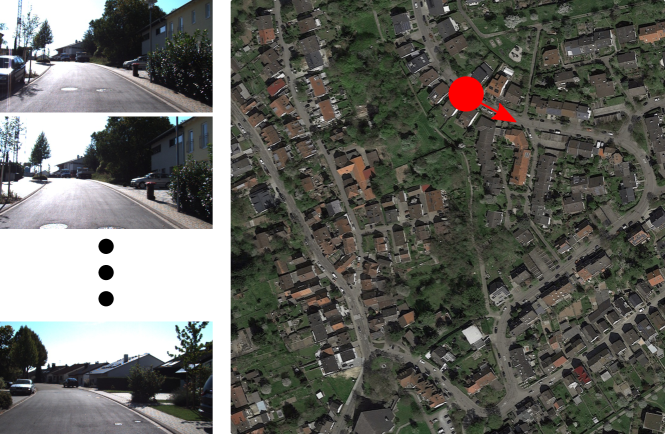
Figure 1: Our model estimates a vehicle’s pose on a georeferenced satellite image (right) given input of a sequence of ground-level images (left).

Satellite imagery provides an alternative source of information that can be employed as a reference for vehicle localization [9, 10, 11, 12, 13]. High resolution, georeferenced, satellite images that densely cover the world are becoming increasingly accessible and well-maintained, as exemplified by Google Maps. The goal is then to perform visual localization using satellite images as the only prior map of the environment. However, registering ground-level images to their corresponding location in a satellite image of the environment is challenging. The difference in their viewpoints means that content visible in one type of image is often not present in the other. For example, whereas ground-level images include building façades and tree trunks, satellite images include roofs and the tops of trees. Additionally, the dynamic nature of the scene means that objects will differ between views. In street scenes, for example, the same parked and stopped cars as well as pedestrians that make up a large fraction of the objects visible at ground-level are not present in satellite views. Meanwhile, satellite imagery may have been acquired at different times of the day and at different times of the year, resulting in appearance variations between ground-level and satellite images due to illumination, weather, and seasons.

In this paper, we describe a framework that employs multi-view learning to perform accurate vision-based localization using satellite imagery as the only prior knowledge of the environment. Our system takes as input a sequence of ground-level images acquired as a vehicle navigates and returns an estimate of its location and orientation in a georeferenced satellite image (Fig. 1). Rather than matching the query images to a prior map of geotagged ground-level images, as is typically done for visual place recognition, we describe a neural multi-view Siamese network that learns to associate novel ground images with their corresponding position and orientation in a satellite image of the scene. We investigate the use of both high-level features, which reduce viewpoint invariance, and mid-level features, which have been shown to exhibit greater invariance to appearance variations [8] as part of our network architecture. As we show, we can train this learned model on ground-satellite pairs from one environment and employ the model in a different environment, without the need for ground-level images for fine-tuning. The framework uses outputs of this learned matching function as observations in a particle filter that maintains a distribution over the vehicle’s pose. In this way, our approach exploits the availability of satellite images to enable visual localization in a manner that is robust to disparate viewpoints and appearance variations, without the need for a prior map of ground-level images. We evaluate our method on the KITTI [14] and St. Lucia [15] datasets, and demonstrate the ability to transfer our learned, hierarchical multi-view model to novel environments and thereby localize the vehicle, despite the challenges of severe viewpoint variations and appearance changes.

II Related Work

The problem of estimating the location of a query ground image is typically framed as one of finding the best match against a database (i.e., map) of geotagged images. In general, existing approaches broadly fall into one of two classes depending on the nature of the query and database images.

II-A Single-View Localization

Single-view approaches assume access to reference databases that consist of geotagged images of the target environment acquired from vantage points similar to that of the query image (i.e., other ground-level images). These databases may come in the form of collections of Internet-based geotagged images, such as those available via photo sharing websites [16, 17, 18] or Google Street View [19, 20], or maintained in maps of the environment (e.g., previously recorded using GPS information or generated via SLAM) [21, 22, 23, 1, 24, 2, 3, 4, 6, 7, 8]. The primary challenges to visual place recognition arise due to variations in viewpoint, variations in appearance that result from changes in environment structure, illumination, and seasons, as well as to perceptual aliasing. Much of the early work attempts to mitigate some of these challenges by using hand-crafted features that exhibit some robustness to transformations in scale and rotation, as well as to slight variations in illumination (e.g., SIFT [25] and SURF [26]), or a combination of visual and textual (i.e., image tags) features [18]. Place recognition then follows as image retrieval, i.e., image-to-image matching-based search against the database [27, 28, 29, 21].

These techniques have proven effective at identifying the location of query images over impressively large areas [17]. However, their reliance upon available reference images limits their use to regions with sufficient coverage and their accuracy depends on the spatial density of this coverage. Further, methods that use hand-crafted interest point-based features tend to fail when faced with significant viewpoint and appearance variations, such as due to large illumination changes (e.g., matching a query image taken at night to a database image taken during the day) and seasonal changes (e.g., matching a query image with snow to one taken during summer). Recent attention in visual place recognition [30, 31, 24, 32, 6, 33, 34, 7, 8] has focused on designing algorithms that exhibit improved invariance to the challenges of viewpoint and appearance variations. Motivated by their state-of-the-art performance on object detection and recognition tasks [35], a solution that has proven successful is to use deep convolutional networks to learn suitable feature representations. Sünderhauf et al. [8] present a thorough analysis of the robustness of different AlexNet [35] features to appearance and viewpoint variations. Based on these insights, Sünderhauf et al. [7] describe a framework that first detects candidate landmarks in an image and then employs mid-level features from a convolutional neural network (AlexNet) to perform place recognition despite significant changes in appearance and viewpoint. We also employ CNNs as a means of learning mid- and high-level features that exhibit improved robustness to viewpoint and appearance variations. Meanwhile, an alternative to single-view matching is to consider image sequences when performing recognition [36, 2, 3, 4, 5], whereby imposing joint consistency reduces the likelihood of false matches and improves robustness to appearance variations.

II-B Cross-View Localization

Cross-view methods identify the location of a query image by matching against a database of images taken from disparate viewpoints. As in our case, this typically involves localizing ground-level images using a database of georeferenced satellite images [9, 10, 11, 12, 12, 37, 38, 39, 13]. Bansal et al. [10] describe a method that localizes street view images relative to a collection of geotagged oblique aerial and satellite images. Their method uses the combination of satellite and aerial images to extract building façades and their locations. Localization then follows by matching these façades against those in the query ground image. Meanwhile, Lin et al. [11] leverage the availability of land use attributes and propose a cross-view learning approach that learns the correspondence between hand-crafted interest-point features from ground-level images, overhead images, and land cover data. Chu et al. [37] use a database of ground-level images paired with their corresponding satellite views to learn a dictionary of color, edge, and neural features that they use for retrieval at test time. Unlike our method, which requires only satellite images of the target environment, both approaches assume access to geotagged ground-level images from the test environment that are used for training and matching.

Viswanathan et al. [12] describe an algorithm that warps 360^∘ view ground images to obtain a projected top-down view that they then match to a grid of satellite locations using traditional hand-crafted features. As with our framework, they use the inferred poses as observations in a particle filter. The technique assumes that the ground-level and satellite images were acquired at similar times, and is thus not robust to the appearance variations that arise as a result of seasonal changes. Viswanathan et al. [13] overcome this limitation by incorporating ground vs. non-ground pixel classifications derived from available LIDAR scans, which improves robustness to seasonal changes. As with their previous work, they also employ a Bayesian filter to maintain an estimate of the vehicle’s pose. In contrast, our method uses only an odometer and a non-panoramic, forward-facing camera with a much narrower field-of-view. Rather than interest point features, we learn to separate location-discriminative feature representations for ground-level and satellite views. These features include an encoding of the scene’s semantic properties, serving a similar role to their ground labels.

Similar to our work is that of Lin et al. [38], who describe a Siamese Network architecture that uses two CNNs to transform ground-level and aerial images into a common feature space. Localizing a query ground image then corresponds to finding the closest georeferenced aerial image in this space. They train their network on a database of ground-aerial pairs and demonstrate the ability to localize test images from environments not encountered during training. Unlike our method, they match against 45^∘ aerial images, which share more content with ground-level images (e.g., building façades) than do satellite views. Additionally, whereas their Siamese network extends AlexNet [35] by using only the second-to-last connected layer (fc7) as the high-level feature, our network adapts VGG-16 [40] with modifications that consider the use of both mid-level and high-level features to improve robustness to changes in appearance.

III Proposed Approach

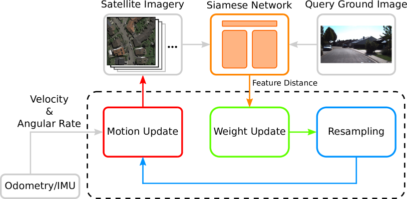
Figure 2: Our method takes as input a stream of ground-level images and maintains a distribution over the vehicle’s pose by comparing these images to a database of satellite images.

Our visual localization framework (Fig. 2) takes as input a stream of ground-level images $\mathcal{I}_{g}^{t}=\{\ldots,I_{t-2},I_{t-1},I_{t}\}$ from a camera mounted to the vehicle and proprioceptive measurements of the vehicle’s motion (e.g., from an odometer and IMU), and outputs a distribution over the vehicle’s pose $x_{t}$ relative to a database of georeferenced satellite images $\mathcal{I}_{s}$, which constitutes the only prior knowledge of the environment. The method consists of a Siamese network that learns feature embeddings suitable to matching ground-level imagery with their corresponding satellite view. These matches then serve as noisy observations of the vehicle’s position and orientation that are then incorporated into a particle filter to maintain a distribution over its pose as it navigates. Next, we describe these components in detail.

III-A Siamese Network

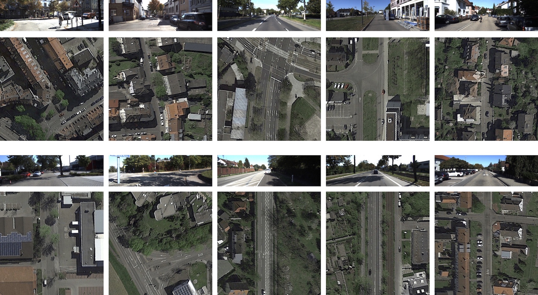
Figure 3: Examples of ground-level images (top rows) paired with their corresponding satellite views (bottom rows). Best viewed in electronic form.

Our method matches a query ground-level image to its corresponding satellite view using a Siamese network [41], which has proven effective at different multi-view learning tasks [42]. Siamese networks consist of two convolutional neural networks (CNNs), one for each of the two disparate views. The two networks operate in parallel, performing nonlinear transformation of their respective input (images) into a common embedding space, constituting a learned feature representations for each view. A query is then matched by finding the nearest cross-view in this embedding space.

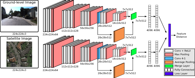
Figure 4: A visualization of our network architecture that consists of two independent CNNs that take as input ground-level and satellite images. Each CNN is an adaptation of VGG-16 CNNs in which mid-level conv4-1 features are downsampled and combined with the output of the last max-pooling layer as the high-level features via summation. The resulting outputs are then used as a measure of distance between ground-level and satellite views.

Our architecture extends a Siamese network to learn location-discriminative feature representations that differentiate between matched ground-satellite pairs and non-matched ground-satellite pairs. The network (Fig. 4) takes as input a pair of ground-level and satellite images that are fed into their respective convolutional neural networks, which output a $d$-dimensional feature embedding ($d=4096$) of each image. As we describe below, the network is trained to discriminate between positive and negative view-pairs using a loss that encourages positive matches to be nearby in the learned embedding space, and features to be distant for non-matching views. Figure 3 presents examples of ground-level images and their matching satellite views, demonstrating the challenging viewpoint and appearance variations. At test time, a query ground-level image is projected into this common space and paired with the satellite view whose embedding is closest in terms of Euclidean distance.

Our network consists of identical CNN architectures for each of the two views that take the form of VGG-16 networks [40], with modifications to improve robustness to variations in appearance. The first modification removes the softmax layer and the last fully connected layer from the original VGG-16 network and adds a batch normalization layer to arrive at the $4096$-dimensional high-level feature representation. The second modification that we consider incorporates additional mid-level features into the learned representation. Mid-level features have been shown to exhibit greater invariance to changes in appearance that result from differences in illumination, weather, and seasons, while high-level output features provide robustness to viewpoint variations [8]. Specifically, we use the output from the conv4-1 layer as the mid-level features and the output from the last max-pooling layer as the high-level feature representation. We note that conv4-1 features of VGG-16 are qualitatively similar to conv3 of AlexNet [35], which Sünderhauf et al. [8] use for place recognition, in terms of their input stimuli [43]. Additionally, high-level features encode semantic information, which is particularly useful for categorizing scenes, while mid-level features tend to be better suited to discriminating between instances of particular scenes. In this way, the two feature representations are complementary. We downsample the conv4-1 mid-level features to match the size of the output from the last max-pooling layer using average-pooling, and combine the two via summation. We evaluate the effect of combining these features in Section IV.

We train our network so as to learn nonlinear transformations of input pairs that bring embeddings of matching ground-level and satellite images closer together, while driving the embeddings associated with non-matching pairs farther apart. To that end, we use a contrastive loss [44]

$$\!\!L(I_{g},I_{s},\ell)=\ell d(I_{g},I_{s})^{2}+(1\!-\ell)\max(m-d(I_{g},I_{s}),0)^{2}$$ (1)

to define the loss between a pair of ground-level $I_{g}$ and satellite $I_{s}$ images, where $\ell$ is a binary-valued correspondence variable that indicates whether the pair match ($\ell=1$), $d(I_{g},I_{s})$ is the Euclidean distance between the image feature embeddings, and $m>0$ is a margin for non-matched pairs.

In the case of matching pairs of ground-level and satellite images $(\ell=1)$, the loss encourages the network to learn feature representations that are nearby in the common embedding space. In the case of non-matching pairs ($\ell=0$), the contrastive loss penalizes the network for transforming the images into features that are separated by a distance less than the margin $m$. In this way, training will tend to pull matching ground-level and satellite image pairs closer together, while keeping non-matching images at least a radius $m$ apart, which provides a form of regularization against trivial solutions [44].

The ground-level and satellite CNN networks can share model parameters or be trained separately. We chose to train the networks with separate parameters for each CNN, but note that previous efforts found little difference with the addition of parameter sharing in similar Siamese networks [38].

III-B Particle Filter

The learned distance function modeled by the convolutional neural network provides a good measure of the similarity between ground-level imagery and the database of satellite views. As a result of perceptual aliasing, however, it is possible that the match that minimizes the distance between the learned features does not correspond to the correct location. In order to mitigate the effect of this noise, we maintain a distribution over the vehicle’s pose as it navigates the environment

$$p(x_{t}|u^{t},z^{t}),$$ (2)

where $x_{t}$ is the pose of the vehicle and $u^{t}=\{u_{0},u_{1},\ldots,u_{t}\}$ denotes the history of proprioceptive measurements (i.e., forward velocity and angular rate). The term $z^{t}=\{z_{0},z_{1},\ldots,z_{t}\}$ corresponds to the history of image-based observations, each consisting of the distance $d(I_{g},I_{s})$ in the common embedding space between the transformed ground-level image $I_{t}$ and the satellite image $I_{s}\in\mathcal{I}_{s}$ with a position and orientation specified by $x_{t}$.

The posterior over the vehicle’s pose tends to be multimodal. Consequently, we represent the distribution using a set of weighted particles

$$\mathcal{P}_{t}=\left\{P_{t}^{(1)},P_{t}^{(2)},\ldots,P_{t}^{(n)}\right\},$$ (3)

where each particle $P_{t}^{(i)}=\{x_{t}^{(i)},w_{t}^{(i)}\}$ includes a sampled vehicle pose $x_{t}^{(i)}$ and the particle’s importance weight $w_{t}^{(i)}$.

We maintain the posterior distribution as new odometry and ground-level images arrive using a particle filter. Figure 2 provides a visual overview of this process. Given the posterior distribution $p(x_{t-1}|u^{t-1},z^{t-1})$ over the vehicle’s pose at time $t-1$, we first compute the prior distribution over $x_{t}$ by sampling from the motion model prior $p(x_{t}|x_{t-1},u^{t},z^{t-1})$, which we model as Gaussian.

After proposing a new set of particles, we update their weights to according to the ratio between the target (posterior) and proposal (prior) distributions

$$\tilde{w}_{t}^{(i)}=p(z_{t}|x_{t},u^{t},z^{t-1})\cdot w_{t-1}^{(i)},$$ (4)

where $\tilde{w}_{t}^{(i)}$ denotes the unnormalized weight at time $t$. We use the output of the Siamese network to define the measurement likelihood as an exponential distribution

$$p(z_{t}|x_{t},u^{t},z^{t-1})=\alpha e^{-\alpha d(I_{t},I_{s})},$$ (5)

where $d(I_{t},I_{s})$ is the Euclidean distance between the CNN embeddings of the current ground-level image $I_{t}$ and the satellite image $I_{s}$ corresponding to pose $x_{t}$, and $\alpha$ is a tuned parameter.

After having calculated and normalized the new importance weights, we periodically perform resampling in order to discourage particle depletion based on the effective number of particles

$$N_{\text{eff}}=\frac{1}{\sum\limits_{i=1}^{N}{w_{t}^{(i)}}^{2}}$$ (6)

Specifically, we use systematic resampling [45] when the effective number of particles $N_{\text{eff}}$ drops below a threshold.

IV Results

We evaluate our model through a series of experiments conducted on two benchmark, publicly available visual localization datasets. We consider two versions of our architecture: Ours-Mid uses both mid- and high-level features, while Ours uses only high-level features. The experiments analyze the ability of our framework to generalize to different test environments and to mitigate appearance variations that result from changes in semantic scene content and illumination.

IV-A Experimental Setup

Our evaluation involves training our network on pairs of ground-level and satellite images from a portion of the KITTI [14] dataset, and testing our method on a different region from KITTI and the St. Lucia dataset [15].

IV-A1 Baselines

We compare the performance of our model against two baselines that consider both hand-crafted and learned feature representations. The first baseline (SIFT) extracts SIFT features [25] from each ground-level and satellite image and computes the distance between a query ground-level image and the extracted satellite image as the average distance associated with the best-matching features. The second baseline (AlexNet-Places) employs a Siamese network comprised of two AlexNet deep convolutional networks [35] trained on the Places dataset [46]. We use the $4096$ dimensional output of the fc7 layer as the embedding when computing the distance used in the measurement update step of the particle filter.

IV-A2 Training Details

Our training data is drawn from the KITTI dataset, collected from a moving vehicle in Karlsruhe, Germany during the daytime in the months of September and October. The dataset consists of sequences that span variations of city, residential, and road scenes. Of these, we randomly sample $18$ sequences from the city, residential, and road categories as the training set, and $5$ from the city and road categories as the validation set, resulting in $14.8$k and $1.3$k ground-level images, respectively.

For each ground-level image in the training and validation sets, we sample a $270\times 400$ ($53\text{\,m}\times 78\text{\,m}$) satellite image at a position $5.0\text{\,m}$ in front of the camera with the long-axis oriented in the direction of the camera. We also include a randomly sampled set of non-matching satellite images. We define a pair of ground-level and satellite images $(I_{g},I_{s})$ to be a match $(\ell=1)$ if their distance is within $4$ m and their orientation within $30$ degrees. We consider non-matches $(\ell=0)$ as those that are more than $80$ m apart. The resulting training set then consists of $538$k pairs ($53$k positive pairs and $485$k negative pairs). Figure 3 presents samples drawn from the set of positive pairs, which demonstrate the challenge of matching these disparate views.

We trained our models from scratch using the contrastive loss (Eqn. 1) with a margin of $m=80$ (tuned on the validation set) using Adam [47] on an Nvidia Titan X. Meanwhile, we used the validation set to tune hyper-parameters including the early stopping criterion, as well as to explore different variations of our network architecture, including alternative methods for combining mid- and high-level features and the use of max-pooling instead of average-pooling.

IV-A3 Particle Filter Implementation

In each experiment, we used $N=5000$ particles representing samples of the vehicle’s position and orientation. We assumed that the vehicle’s initial pose was unknown (i.e., the kidnapped robot setting), and biased the initialization of each filter such that samples were more likely to be drawn on roadways. Particles were resampled using $N_{\text{eff}}=0.8N$ (tuned on a validation set). We determine a filter to have converged when the standard deviation of the estimates is less than $10$ m.

IV-B Experimental Results

We evaluate two versions of our method against the different baselines with regards to the effects of appearance variations due to changes in viewpoint, location, scene content, and illumination both between training and test as well as between the reference satellite and ground-level imagery. We analyze the performance in terms of precision-recall as well as retrieval. We then investigate the accuracy with which the particle filter is able to localize the vehicle as it navigates.

IV-B1 KITTI Experiment

We evaluate our method on KITTI using two residential sequences (KITTI-Test-A and KITTI-Test-B) as test sets. We note that there is no environment overlap between these sequences and those used for training or validation. The georeferenced satellite maps for KITTI-Test-A is $0.80\,\text{km}\times 1.10\,\text{km}$ and $0.53\,\text{km}\times 0.70\,\text{km}$ for KITTI-Test-B.

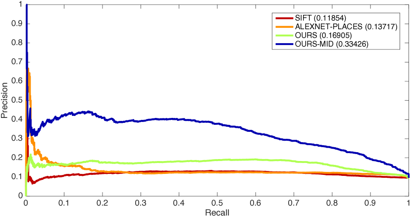
(a) Precision-Recall

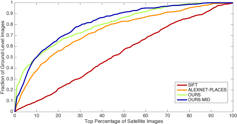
(b) Retrieval Accuracy

Figure 5: Results on the KITTI test set including 5(a) precision-recall curves with the average precision values in parentheses and 5(b) retrieval accuracy.

Figure 5(a) compares the precision-recall curve of our models against the two baseline for the two KITTI test sequences. The plot additionally includes the average precision for each model. The plot shows that Ours-Mid is the most effective at matching ground-level images with their corresponding satellite views. The use of a contrastive loss as a means of encouraging our network to bring positive pairs closer together facilitates accurate matching. Comparing against the performance of Ours demonstrates that the incorporation of mid-level features helps to mitigate the effects of appearance variations. Meanwhile, the AlexNet-Places baseline that uses the output of AlexNet trained on Places as the learned feature embeddings outperforms the SIFT baseline that relies upon hand-designed SIFT features to identify correspondences.

As another measure of the discriminative ability of our network architecture, we consider the frequency with which the correct satellite view is in the top-$X\%$ matches for a given ground-level image according to the feature embedding distance. Figure 5(b) plots the fraction of query ground-level images for which the corresponding satellite view is found in the top-$X\%$ of the satellite images. In the case of both Ours-Mid and Ours, the correct satellite view is in the top $10\%$ for more than $50\%$ of the ground-level images. When we increase the size of the candidate set, our method yields a slight increase in performance (around $4\%$). The AlexNet-Places baseline performs slightly worse, while all three significantly outperform the SIFT baseline, which is essentially equivalent to chance.

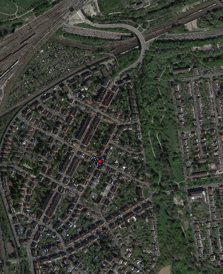
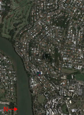
Figure 6: Particle filter localization for KITTI-Test-A (left), KITTI-Test-B (center), and St-Lucia (right) with blue circles denoting the position associated with each particle. The green and red circles indicate the mean position estimate and ground-truth, respectively. Note that St-Lucia is rotated.

TABLE I: Final mean position error and standard deviation (in meters)

	KITTI-Test-A	KITTI-Test-B	St-Lucia
SIFT	$656.70$ ($244.29$)	$243.08$ ($79.63$)	$554.35$ ($17.26$)
AlexNet-Places	$177.82$ $0$($25.68$)	$59.95$ ($38.99$)	$77.15$ ($52.61$)
Ours	$8.41$ ($5.56$)	$7.93$ ($2.14$)	$\mathbf{26.38}$ ($5.63$)
Ours-Mid	$\mathbf{7.69}$ ($5.14$)	$\mathbf{4.65}$ ($2.77$)	$35.81$ ($7.54$)

Next, we evaluate our method’s ability to estimate the vehicle’s pose as it navigates the environment by using the distance between the learned feature representations as observations in the particle filter. In Table I, we report the quantitative results for each of the two KITTI test environments. Note that the final position mean error and standard deviation is measured at the last ground-level image sequence using all of the particles. Figure 6 depicts the converged particle filter estimate of the vehicle’s position using Ours-Mid compared to the ground-truth position. For both KITTI-Test-A and KITTI-Test-B, the filter that uses Ours-Mid has smaller average position errors, compared to the one that uses Ours. Using Ours-Mid, the filter converged at $55.62$ s and $62.25$ s for KITTI-Test-A and KITTI-Test-B, respectively, and using Ours, the filter converged at $64.67$ s and $70.15$ s for KITTI-Test-A and KITTI-Test-B, respectively. Meanwhile, the SIFT baseline failed to converge with large average errors for both KITTI-Test-A and KITTI-Test-B. The AlexNet-Places baseline faired better, but the filter also did not converge for either of the test sets. The results support the argument that our method’s ability to learn mid- and high-level feature representations with a loss that brings ground-level image embeddings closer to their corresponding satellite representation results in measurements that are able to distinguish between correct and incorrect matches.

IV-B2 St. Lucia Experiment

Next, we consider the St. Lucia dataset [15] as a means of evaluating the method’s ability to generalize the model trained on KITTI to new environments with differing semantic content. The dataset was collected during August from a car driving through a suburb of Brisbane, Australia at different times during a single day and over different days during a two week period. We use the dataset collected on August $21$ at $12$:$10$ as the validation set and the dataset collected on August $19$ at $14$:$10$ as the test set. The two exhibit slight variations in viewpoint due to differences in the vehicle’s route. More pronounced appearance variations result from illumination changes and non-stationary objects in the environment (e.g., cars and pedestrians). Note that the dataset does not include the vehicle’s velocity or angular rate. As done elsewhere [31] we simulate visual odometry by interpolating the GPS differential, which is prone to significant noise and is thereby representative of the quality of data that visual odometry would yield. The georeferenced satellite map is $1.8$ km $\times 1.2$ km.

Table I compares the performance on the St. Lucia dataset. Figure 6 (right) presents the converged particle filter estimate maintained using our method (Ours-Mid), along with the ground-truth vehicle location during the run. Despite the viewpoint and appearance variations relative to the training set and between the ground-level and satellite views, both the filters using Ours-Mid and Ours maintain a converged estimate of the vehicle’s pose. The filter associated with Ours-Mid resulted in a larger final position error than that associated with Ours. Using Ours-Mid, the filter converged $17\%$ faster than that using Ours. Both the SIFT and AlexNet-Places baselines failed to converge.

IV-B3 Computational Efficiency

As with other approaches to visual localization [48, 7], the current implementation of our framework does not process images in real-time. Computing the CNN feature representations for a pair of ground-level and satellite images requires approximately $55$ ms on an Nvidia Titan X, though the two network components can be decoupled, thereby requiring that each ground-level image be embedded only once, which reduces overall computational cost. For the experiments presented in this paper, we cropped and processed the satellite image associated with each particle at every update step. This process can be made significantly more efficient by pre-processing satellite images corresponding to a discrete set of poses, in which case the primary cost is that of computing the ground-level image embeddings. Empirical results demonstrate that this results in a negligible decrease in accuracy.

V Conclusion

We described a method that is able to localize a ground vehicle by exploiting the availability of satellite imagery as the only prior map of the environment. Underlying our framework is a multi-view neural network that learns to match ground-level images with their corresponding satellite view. The architecture enables our method to learn feature representations that help to mitigate the challenge of severe viewpoint variation and that improve robustness to appearance variations resulting from changes in illumination and scene content. Distances in this common embedding space then serve as observations in a particle filter that maintain an estimate of the vehicle’s pose. We evaluate our model on benchmark visual localization datasets and demonstrate the ability to transfer our learned multi-view model to novel environments. Future work includes adaptations to the mult-view model that tolerate more severe appearance variations (e.g., due to seasonal changes).

VI Acknowledgements

We thank the NVIDIA corporation for the donation of Titan X GPUs used in this research.

References

- Churchill and Newman [2012] W. Churchill and P. Newman, “Practice makes perfect? Managing and leveraging visual experiences for lifelong navigation,” in Proc. IEEE Int’l Conf. on Robotics and Automation (ICRA), 2012.
- Milford and Wyeth [2012] M. J. Milford and G. F. Wyeth, “SeqSLAM: Visual route-based navigation for sunny summer days and stormy winter nights,” in Proc. IEEE Int’l Conf. on Robotics and Automation (ICRA), 2012.
- Johns and Yang [2013] E. Johns and G.-Z. Yang, “Feature co-occurrence maps: Appearance-based localisation throughout the day,” in Proc. IEEE Int’l Conf. on Robotics and Automation (ICRA), 2013.
- Sünderhauf et al. [2013] N. Sünderhauf, P. Neubert, and P. Protzel, “Are we there yet? Challenging SeqSLAM on a 3000 km journey across all four seasons,” in Proc. ICRA Work. on Long-Term Autonomy, 2013.
- Naseer et al. [2014] T. Naseer, L. Spinello, W. Burgard, and C. Stachniss, “Robust visual robot localization across seasons using network flows,” in Proc. Nat’l Conf. on Artificial Intelligence (AAAI), 2014.
- McManus et al. [2014a] C. McManus, W. Churchill, W. Maddern, A. D. Stewart, and P. Newman, “Shady dealings: Robust, long-term visual localisation using illumination invariance,” in Proc. IEEE Int’l Conf. on Robotics and Automation (ICRA), 2014.
- Sünderhauf et al. [2015a] N. Sünderhauf, S. Shirazi, A. Jacobson, F. Dayoub, E. Pepperell, B. Upcroft, and M. Milford, “Place recognition with ConvNet landmarks: Viewpoint-robust, condition-robust, training-free,” in Proc. Robotics: Science and Systems (RSS), 2015.
- Sünderhauf et al. [2015b] N. Sünderhauf, F. Dayoub, S. Shirazi, B. Upcroft, and M. Milford, “On the performance of ConvNet features for place recognition,” in Proc. IEEE/RSJ Int’l Conf. on Intelligent Robots and Systems (IROS), 2015.
- Jacobs et al. [2007] N. Jacobs, S. Satkin, N. Roman, and R. Speyer, “Geolocating static cameras,” in Proc. Int’l Conf. on Computer Vision (ICCV), 2007.
- Bansal et al. [2011] M. Bansal, H. S. Sawhney, H. Cheng, and K. Daniilidis, “Geo-localization of street views with aerial image databases,” in Proc. ACM Int’l Conf. on Multimedia (MM), 2011.
- Lin et al. [2013] T.-Y. Lin, S. Belongie, and J. Hays, “Cross-view image geolocalization,” in Proc. IEEE Conf. on Computer Vision and Pattern Recognition (CVPR), 2013.
- Viswanathan et al. [2014] A. Viswanathan, B. R. Pires, and D. Huber, “Vision based robot localization by ground to satellite matching in GPS-denied situations,” in Proc. IEEE/RSJ Int’l Conf. on Intelligent Robots and Systems (IROS), 2014.
- Viswanathan et al. [2016] ——, “Vision-based robot localization across seasons and in remote locations,” in Proc. IEEE Int’l Conf. on Robotics and Automation (ICRA), 2016.
- Geiger et al. [2013] A. Geiger, P. Lenz, C. Stiller, and R. Urtasun, “Vision meets robotics: The KITTI dataset,” Int’l J. of Robotics Research, vol. 32, no. 11, 2013.
- Warren et al. [2010] M. Warren, D. McKinnon, H. He, and B. Upcroft, “Unaided stereo vision based pose estimation,” in Proc. Australasian Conf. on Robotics and Automation, 2010.
- Zhang and Kosecka [2006] W. Zhang and J. Kosecka, “Image based localization in urban environments,” in Proc. Int’l Symp. on 3D Data Processing, Visualization, and Transmission, 2006.
- Hays and Efros [2008] J. Hays and A. A. Efros, “IM2GPS: Estimating geographic information from a single image,” in Proc. IEEE Conf. on Computer Vision and Pattern Recognition (CVPR), 2008.
- Crandall et al. [2009] D. J. Crandall, L. Backstrom, D. Huttenlocher, and J. Kleinberg, “Mapping the world’s photos,” in Proc. Int’l World Wide Web Conf. (WWW), 2009.
- Zamir and Shah [2010] A. R. Zamir and M. Shah, “Accurate image localization based on Google Maps Street View,” in Proc. European Conf. on Computer Vision (ECCV), 2010.
- Majdik et al. [2013] A. L. Majdik, Y. Albers-Schoenberg, and D. Scaramuzza, “MAV urban localization from Google Street View data,” in Proc. IEEE/RSJ Int’l Conf. on Intelligent Robots and Systems (IROS), 2013.
- Schindler et al. [2007] G. Schindler, M. Brown, and R. Szeliski, “City-scale location recognition,” in Proc. IEEE Conf. on Computer Vision and Pattern Recognition (CVPR), 2007.
- Cummins and Newman [2008] M. Cummins and P. Newman, “FAB-MAP: Probabilistic localization and mapping in the space of appearance,” International Journal of Robotics Research, vol. 27, no. 6, 2008.
- Chen et al. [2011] D. M. Chen, G. Baatz, K. Köser, S. S. Tsai, R. Vedantham, T. Pylvänäinen, K. Roimela, X. Chen, J. Bach, M. Pollefeys, B. Girod, and R. Grzeszczuk, “City-scale landmark identification on mobile devices,” in Proc. IEEE Conf. on Computer Vision and Pattern Recognition (CVPR), 2011.
- Badino et al. [2012] H. Badino, D. Huber, and T. Kanade, “Real-time topometric localization,” in Proc. IEEE Int’l Conf. on Robotics and Automation (ICRA), 2012.
- Lowe [2004] D. G. Lowe, “Distinctive image features from scale-invariant keypoints,” Int’l J. on Computer Vision, vol. 60, no. 2, 2004.
- Bay et al. [2006] H. Bay, T. Tuytelaars, and L. Van Gool, “Surf: Speeded up robust features,” in Proc. European Conf. on Computer Vision (ECCV), 2006.
- Wolf et al. [2005] J. Wolf, W. Burgard, and H. Burkhardt, “Robust vision- based localization by combining an image-retrieval system with monte carlo localization,” Trans. on Robotics, vol. 21, no. 2, 2005.
- Li and Kosecka [2006] F. Li and J. Kosecka, “Probabilistic location recognition using reduced feature set,” in Proc. IEEE Int’l Conf. on Robotics and Automation (ICRA), 2006.
- Filliat [2007] D. Filliat, “A visual bag of words method for interactive qualitative localization and mapping,” in Proc. IEEE Int’l Conf. on Robotics and Automation (ICRA), 2007.
- Valgren and Lilienthal [2007] C. Valgren and A. J. Lilienthal, “SIFT, SURF and seasons: Long-term outdoor localization using local features,” in Proc. European Conf. on Mobile Robotics (ECMR), 2007.
- Glover et al. [2010] A. J. Glover, W. P. Maddern, M. J. Milford, and G. F. Wyeth, “FAB-MAP + RatSLAM: Appearance-based SLAM for multiple times of day,” in Proc. IEEE Int’l Conf. on Robotics and Automation (ICRA), 2010.
- Neubert et al. [2013] P. Neubert, N. Sünderhauf, and P. Protzel, “Appearance change prediction for long-term navigation across seasons,” in Proc. European Conf. on Mobile Robotics (ECMR), 2013.
- Maddern et al. [2014] W. Maddern, A. Stewart, C. McManus, B. Upcroft, W. Churchill, and P. Newman, “Transforming morning to afternoon using linear regression techniques,” in Proc. IEEE Int’l Conf. on Robotics and Automation (ICRA), 2014.
- Lowry et al. [2014] S. M. Lowry, M. J. Milford, and G. F. Wyeth, “Transforming morning to afternoon using linear regression techniques,” in Proc. IEEE Int’l Conf. on Robotics and Automation (ICRA), 2014.
- Krizhevsky et al. [2012] A. Krizhevsky, I. Sutskever, and G. E. Hinton, “ImageNet classification with deep convolutional neural networks,” in Adv. Neural Information Processing Systems (NIPS), 2012.
- Koch et al. [2010] O. Koch, M. R. Walter, A. Huang, and S. Teller, “Ground robot navigation using uncalibrated cameras,” in Proc. IEEE Int’l Conf. on Robotics and Automation (ICRA), 2010.
- Chu et al. [2015] H. Chu, H. Mei, M. Bansal, and M. R. Walter, “Accurate vision-based vehicle localization using satellite imagery,” arXiv:1510.09171, 2015.
- Lin et al. [2015] T.-Y. Lin, Y. Cui, S. Belongie, and J. Hays, “Learning deep representations for ground-to-aerial geolocalization,” in Proc. IEEE Conf. on Computer Vision and Pattern Recognition (CVPR), 2015.
- Workman et al. [2015] S. Workman, R. Souvenir, and N. Jacobs, “Wide-area image geolocalization with aerial reference imagery,” in Proc. Int’l Conf. on Computer Vision (ICCV), 2015.
- Simonyan and Zisserman [2015] K. Simonyan and A. Zisserman, “Very deep convolutional networks for large-scale image recognition,” in Proc. Int’l Conf. on Learning Representations (ICLR), 2015.
- Chopra et al. [2005] S. Chopra, R. Hadsell, and Y. LeCun, “Learning a similarity metric discriminatively, with application to face verification,” in Proc. IEEE Conf. on Computer Vision and Pattern Recognition (CVPR), 2005.
- Taigman et al. [2014] Y. Taigman, M. Yang, M. Ranzato, and L. Wolf, “DeepFace: Closing the gap to human-level peformance in face verification,” in Proc. IEEE Conf. on Computer Vision and Pattern Recognition (CVPR), 2014.
- Zeiler and Fergus [2014] M. D. Zeiler and R. Fergus, “Visualizing and understanding convolutional networks,” in Proc. European Conf. on Computer Vision (ECCV), 2014.
- Hadsell et al. [2006] R. Hadsell, S. Chopra, and Y. LeCun, “Dimensionality reduction by learning an invariant mapping,” in Proc. IEEE Conf. on Computer Vision and Pattern Recognition (CVPR), 2006.
- Carpenter et al. [1999] J. Carpenter, P. Clifford, and P. Fearnhead, “Improved particle filter for nonlinear problems,” in Proc. Radar, Sonar, and Navigation, vol. 146, no. 1, 1999.
- Zhou et al. [2014] B. Zhou, A. Lapedriza, J. X. nd A. Torralba, and A. Oliva, “Learning deep features for scene recognition using the Places database,” in Adv. Neural Information Processing Systems (NIPS), 2014.
- Kingma and Ba [2015] D. Kingma and J. Ba, “Adam: A method for stochastic optimization,” in Proc. Int’l Conf. on Learning Representations (ICLR), 2015.
- McManus et al. [2014b] C. McManus, B. Upcroft, and P. Newman, “Scene signatures: Localised and point-less features for localisation,” in Proc. Robotics: Science and Systems (RSS), 2014.