figurec

See pages - of LukesSOFI2017ms.pdf

Supplementary Material for the article:

Quantifying protein densities on cell membranes using super-resolution optical fluctuation imaging

Tomáš Lukeš^1,2, Daniela Glatzová^3,4, Zuzana Kvíčalová³, Florian Levet^5,6, Aleš Benda^3,7,Tomáš Brdička⁴, Theo Lasser¹ & Marek Cebecauer<sup>3

1</sup>Laboratoire d’Optique Biomédicale, Ecole Polytechnique Fédérale de Lausanne, Lausanne, Switzerland
²Department of Radioelectronics, Faculty of Electrical Engineering, Czech Technical University in Prague, Prague, Czech Republic
³J. Heyrovsky Institute of Physical Chemistry, Academy of Sciences, Prague, Czech Republic
⁴Institute of Molecular Genetics, Czech Academy of Sciences, Prague, Czech Republic
⁵Interdisciplinary Institute for Neuroscience, UMR 5297 CNRS, Université de Bordeaux,
Bordeaux, France
⁶Bordeaux Imaging Center, UMS 3420 CNRS, Université de Bordeaux, US4 INSERM,
Bordeaux, France
⁷Imaging methods core facility, BIOCEV, Vestec u Prahy, Czech Republic

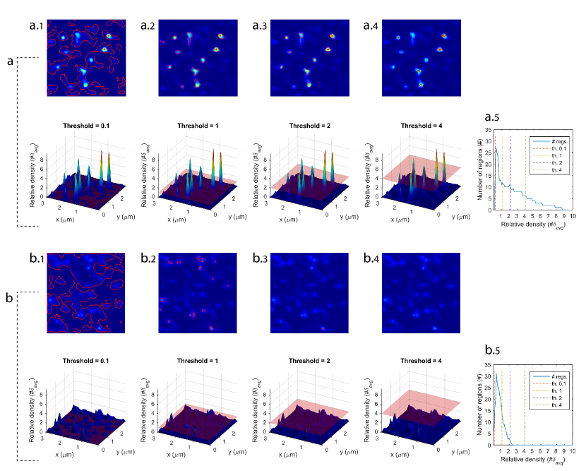
Figure 1:

SOFI-based molecular density analysis - threshold filtering.

Threshold filtering of simulated datasets containing (a) high density clusters, (b) randomly distributed emitters. First a mean density over the wall region of interests (ROIs) is calculated as $\delta_{\mathrm{avg}}=\frac{1}{KLN}\sum_{k=1}^{K}\sum_{l=1}^{N}\sum_{n=1}^{N}d(k,l,n)$, where $d(k,l,n)$ is a molecular density per pixel located in the k-th row and l-th column of n-th ROI, N is the total number of ROIs, k,l runs through all rows and columns of the ROI, respectively. The threshold parameter is given as a multiple of the mean density taken over the selected ROI. i.e. $threshold=2$ corresponds to $2\delta_{\mathrm{avg}}$. For each threshold setting, densities above the threshold determine the boundary of the density dependent area providing number of segments, area size and equivalent diameter. (a.1 - a.4) shows an example for threshold values: 0.1, 1, 2, and 4. Repeating this procedure step by step for the whole range of thesholds, we obtain charts that show number of HDRs as a function of the density threshold (a.5,b.5; blue line) for the case with HDRs (a.5) and with randomly distributed molecules (b.5). For the first case, 6 HDRs are detected at the density threshold 4 (a.5; green dashed line). For the second case, 0 HDRs is detected at this density threshold (b.5; green dashed line).

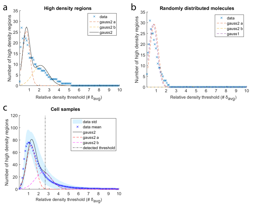
Figure 2:

SOFI-based molecular density analysis - threshold detection.

Number of high density regions (HDRs) as a function of density threshold for a simulated sample which (a) contains high density regions, or (b) contains randomly distributed molecules. Fitting a sum of two Gaussian functions reveals a component which corresponds to the random patterns (red dashed line) and a component corresponding to non random HDRs (yellow dashed line). (c) Number of HDRs as a function of density threshold averaged over all cell samples (i.e. 80 samples). Averaging across all samples allows us to obtain one density threshold for all samples and thus compare HDRs size of different CD4 variants at the same density level (Fig. 3). A sum of two Gaussian functions fitted to the data ("gauss2"). Vertical dash-dot line indicates the detected threshold where the value of the Gaussian function (red dashed line), which corresponds to randomly distributed molecules, falls below 1.

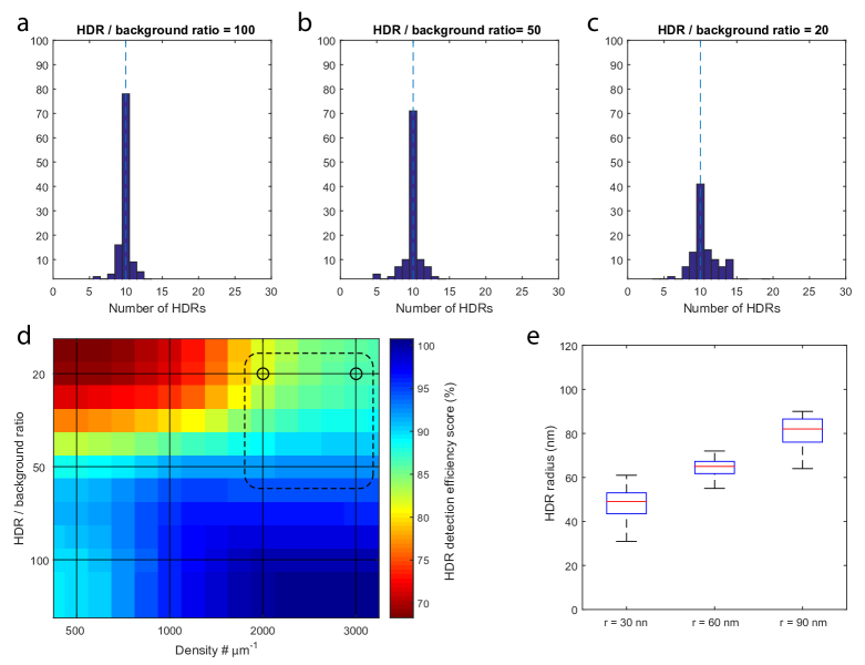
Figure 3:

Simulation of SOFI-based molecular density analysis under controlled conditions.

Estimation of number of high density regions (HDRs): 10 simulated HDR per ROI as ground truth. The HDR radius was in the range $\{30,60,90\}$ nm, the molecular density per cluster was in the range $\{500,1000,2000,3000\}$ molecules per $\mu m^{2}$. In between the HDRs, molecules were randomly distributed such that HDR/background ratio was equal to $\{100,50,20\}$. Each test scenario was repeated 10 times. In total, 360 datasets were generated and evaluated (120 datasets for each HDR/background case). The number of photons per emitter per frame was set to 100, which corresponds well to the experimental conditions. The number of frames of each image sequence was 5000. Dashed blue line in (a),(b),(c) marks the ground truth.
Overall, the simulation validates the algorithm and estimation under a broad range of conditions. (d) HDR detection efficiency score is a probability that the estimated number of HDRs is in the range (7-13). The accuracy of the estimation increases with increasing HDR/background ratio and increasing HDR density. The simulations were calculated for the grid points. The dashed line marks the conditions where the signal to noise ratio (SNR) and signal to background ratio (SBR) of simulated data correspond to SNR and SBR of the real cell datasets in our experiments. (e) Estimation of HDR radius for grid points marked in d by the circles.

Figure 4: Schematic representation of wild-type (WT) CD4 and its variants: palmitoylation mutant (CS1), mutant missing the extracellular domain (dD1D4) and mutant missing the intracellular domain (dCT). TM = transmembrane domain, Ig = four immunoglobulin type domains D1-D4, Palm = palmitoylations sites C419 and C422, Non-palm = non-palmitoylated variant with mutations C419,422S. Proportions are not in scale.

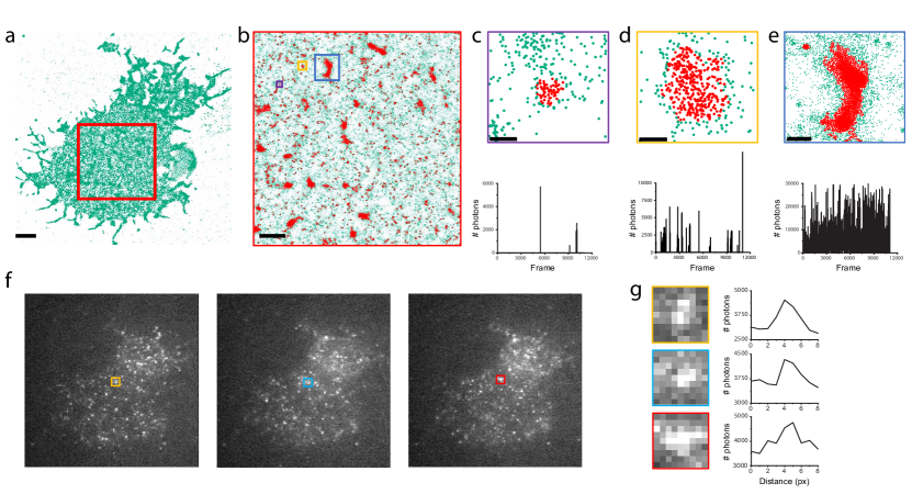
Figure 5:

SMLM analysis of the plasma membrane organisation of CD4 variants.

Plasma membrane organisation of the CD4 protein variants in resting T cells characterized using photo-activation localisation microscopy (PALM) followed by a Voronoï-based segmentation algorithm [1]. High density regions (HDRs) of irregular shape frequently forming networks of connected areas are identified. Yet, since the acquisition exhibited a high density of molecules with high blinking rates, the quantification of these HDRs can be affected by localization errors and under- or overcounting artifacts as described by Burgert et al. [2]. (a) Original dataset composed of 1,747,681 localizations, scale bar 2 $\mu$m. (b) Magnification of the central area of the cell. Segmented HDRs are displayed in red, scale bar 1 $\mu$m. (c) Zoom on a HDR composed of 65 localizations, scale bar 50 nm. As shown by its time trace, the localizations in this region are originating from a single fluorophore, making its blinking correction simple. (d-e) Zoom on a denser HDR (d, 384 localizations, scale bar 50 nm) and interconnected HDRs (e, 12,886 localizations, scale bar 200 nm) with their time trace. Even for a small HDR, the presence of multiple emitters complicates the blinking correction. The problem becomes even more apparent with interconnected HDRs because of their high-density of molecules. (f-g) Three frames of the original image acquisition, pixel size 105 nm. (g) Corresponding zoom to the region covered by one HDR. The high-density of molecules makes it difficult to properly separate each emitter, resulting in localization errors as well as under-counting.

Figure 6: Each row represents four selected ROIs of one CD4 variant. Colorbar represents relative density ($\#\delta_{avg}$). Scale bar 500 nm.

Supplementary Note: SOFI density estimation

The technical requirements for SOFI are a classical widefield microscope merged with a fast high sensitivity digital camera. SOFI image processing is based on higher order statistics and exploits the temporal sequence of blinking fluorescent emitters [3, 4]. Calculating spatio-temporal cross-cumulants allows SOFI to obtain a super-resolved, background-free and noise-reduced images. Higher-order cumulants contain information about the photo-physics of the emitters. Combining SOFI images of different cumulant orders, allows one to extract physical parameters like molecular density [5], which we applied to investigate plasma membrane distribution of proteins.

1.1 SOFI principle and theory

As stated by Dertinger et al. [3], the fluctuating emitters should switch between at least two optically distinguishable states (e.g. a dark and a bright state) repeatedly and independently in a stochastic manner. Images of stochastically blinking emitters are recorded such that the point-spread function (PSF) extends over several camera pixels. Acquiring a sequence of images results in a time dependent intensity trace for each pixel. Assuming N independently fluctuating emitters, the detected intensity is given as

$$I(\mathbf{r},t)=\sum_{k=1}^{N}\epsilon_{k}U(\mathbf{r-r}_{k})s_{k}(t)+b(\mathbf{r})+n(\mathbf{r},t),$$ (1)

where $\epsilon_{k}$ is the molecular brightness, $U(\mathbf{r-r}_{k})$ is the PSF at the position $\mathbf{r}_{k}$, $s_{k}(t)$ denotes a switching function (normalized fluctuation sequence, $s_{k}(t)\in\{0,1\}$), $b(\mathbf{r})$ is a constant background, and $n(\mathbf{r},t)$ represents an additive noise contribution.

For each pixel, an $n^{th}$ order cumulant is calculated for disentangling emitters inside the PSF. By applying the $n^{th}$ order cumulant to Eq. (1), we obtain

$${\kappa{}}_{n}\{I(\mathbf{r},t)\}(\tau{})={\kappa{}}_{n}\left\{\sum_{k=1}^{M}{\epsilon{}}_{k}U(\mathbf{r}-{\mathbf{r}}_{k})s_{k}(t)+b(\mathbf{r})+n(\mathbf{r},t)\right\}(\tau{}).$$ (2)

Using additivity and semi-invariance properties of cumulants [6], the $n^{th}$ order cumulant with zero time lag can be written as

$$\kappa_{n}\{I(\mathbf{r},t)\}=\sum_{k=1}^{N}\epsilon_{k}^{n}U^{n}(\mathbf{r-r}_{k})\kappa_{n}\{s_{k}(t)\}+\kappa_{n}\{b(\mathbf{r})\}+\kappa_{n}\{n(\mathbf{r},t)\}.$$ (3)

For ($n\geq 2$), the Gaussian noise ($\kappa\{n(\mathbf{r},t)\}$)) and stationary background ($\kappa\{b(\mathbf{r})\}$ ) terms are eliminated by the cumulant analysis as an intrinsic property of cumulants. For an $n^{th}$ order cumulant, the PSF is raised to the $n^{th}$ power (see Eq. 3). As a consequence, the PSF is narrowed and the spatial resolution is improved by a factor of $\sqrt{n}$ [3]. Therefore, increasing the cumulant order yields an image with an enhanced spatial resolution. Since a multiplication in the spatial domain corresponds to a convolution in the frequency domain, the cut-off frequency of the spectrum $\tilde{U}^{n}\left(\mathbf{k}\right)$ is n-times higher than that of $\tilde{U}\left(\mathbf{k}\right)$. By applying a deconvolution and a subsequent rescaling, the $n^{th}$ order cumulant image exhibits an up to n-fold resolution improvement [4]. As shown in [4], virtual pixels can be calculated in between the physical pixels using cross-cumulants and followed by a flattening operation i.e. assigning proper weights to these virtual pixels [4, 7, 8].

SOFI assumes a blinking model where the fluorophores reversibly switch between a bright and a dark state. In Deschout et al. [9], SOFI was applied to the PALM photo-physical model. In the PALM photo-physical model, the emitter activation is assumed as non-reversible, however, once the emitter is activated, it exhibits several fast blinking events prior to the final bleaching event [10]. The emitter fluctuates between two different states (an on-state $S_{\mathrm{on}}$ and a dark state $S_{\mathrm{off}}$), which is expressed by the on-time ratio as

$$\rho=\frac{\tau_{\mathrm{on}}}{\tau_{\mathrm{on}}+\tau_{\mathrm{off}}},$$ (4)

where $\tau_{\mathrm{on}}$ and $\tau_{\mathrm{off}}$ are the characteristic lifetimes of the $S_{\mathrm{on}}$ and $S_{\mathrm{off}}$ states. The $n^{th}$ order cumulant $\kappa_{n}\{s_{k}(t)\}$ is in this model described by a Bernoulli distribution with probability $\rho_{\mathrm{on}}$ [5] and approximated by an $n^{th}$ order polynomial function for the on-time ratio as

$$f_{n}(\rho_{\mathrm{on}})=\rho_{\mathrm{on}}(1-\rho_{\mathrm{on}})\frac{\partial f_{n-1}}{\partial\rho_{\mathrm{on}}}.$$ (5)

Under these conditions, the $n^{th}$ order cumulant can be approximated as [5]

$$\kappa_{n}\{I(\mathbf{r,t})\}\approx\epsilon^{n}f_{n}(\rho_{\mathrm{on}})\sum_{k=1}^{N}U^{n}(\mathbf{r-r}_{k}).$$ (6)

1.2 Estimation of density maps

Geissbuehler et al. [5] used three cumulant images ($2^{\text{nd}}$, $3^{\text{rd}}$, and $4^{\text{th}}$ order) to estimate molecular parameters: on-time ratio, brightness and molecular density. Here, we generalize this concept to any three cumulant images of distinct orders. If we assume spatially varying but locally constant on-time ratios and molecular brightness, the cumulants (for the cumulant order $n>1$) can be approximated by [5]

$$g_{n}(\mathbf{r})\approx\epsilon^{n}(\mathbf{r})f_{n}(\rho_{\mathrm{on}})N(\mathbf{r})\mathcal{E}_{V}\{U^{n}(\mathbf{r})\}.$$ (7)

where $\mathcal{E}_{V}\{U^{n}(\mathbf{r})\}$ is the expectation value of $U^{n}(\mathbf{r})$, $N(\mathbf{r})$ is the number of emitters inside a detection volume V. Approximating the PSF near the interface in a total internal reflection (TIR) configuration by a lateral 2D Gaussian profile combined with an axial exponential profile, we obtain

$$\mathcal{E}_{V}\{U_{\mathrm{TIR}}^{n}(\mathbf{r})\}=\frac{c(\sigma_{x,y},\sigma_{z},d_{z})}{n^{2}},$$ (8)

where $d_{z}$ represents the exponential decay of the TIR illumination [11].

Using 3 consecutive cumulant images of orders $n,(n-1),(n-2)$, we obtain for the ratios

$$K_{1}=\frac{g_{n-1}}{g_{n-2}}=\frac{f_{n-1}(\rho_{\mathrm{on}}(\mathbf{r}))}{f_{n-2}(\rho_{\mathrm{on}}(\mathbf{r}))}\epsilon(\mathbf{r})\frac{\mu_{n-1}}{\mu_{n-2}}$$ (9)

$$K_{2}=\frac{g_{n}}{g_{n-2}}=\frac{f_{n}(\rho_{\mathrm{on}}(\mathbf{r}))}{f_{n-2}(\rho_{\mathrm{on}}(\mathbf{r}))}\epsilon^{2}(\mathbf{r})\frac{\mu_{n}}{\mu_{n-2}}$$ (10)

$$K_{3}=\frac{g_{n}}{g_{n-1}}=\frac{f_{n}(\rho_{\mathrm{on}}(\mathbf{r}))}{f_{n-1}(\rho_{\mathrm{on}}(\mathbf{r}))}\epsilon(\mathbf{r})\frac{\mu_{n}}{\mu_{n-1}},$$ (11)

where $\mu_{n}=\mathcal{E}_{V}\{U^{n}(\mathbf{r})\}$. Substitution of Eq. (11) into Eq. (9) leads to

$$\frac{g_{n}g_{n-2}}{g_{n-1}^{2}}=\frac{f_{n}(\rho_{\mathrm{on}}(\mathbf{r}))f_{n-2}(\rho_{\mathrm{on}}(\mathbf{r}))}{f_{n-1}^{2}(\rho_{\mathrm{on}}(\mathbf{r}))}.$$ (12)

$$\left\{\epsilon(\mathbf{r})=\frac{g_{n}}{g_{n-1}}\frac{f_{3}(\rho_{\mathrm{on}}(\mathbf{r}))}{f_{n}(\rho_{\mathrm{on}}(\mathbf{r}))}\frac{\mu_{n-1}}{\mu_{n}},N(\mathbf{r})=\frac{g_{n}(\mathbf{r})}{\epsilon^{n}(\mathbf{r})f_{n}(\rho_{\mathrm{on}})\mu_{n}}\right\}.$$ (13)

Building up the ratios $K_{1}$ and $K_{2}$ from the Eq. (14) for cumulants of $2^{nd},3^{rd},$ and $4^{th}$ order, we obtain

$$K_{1}(\mathbf{r})=\frac{\mu_{2}g_{3}}{\mu_{3}g_{2}}(\mathbf{r})=\epsilon(\mathbf{r})(1-2\rho_{\mathrm{on}}(\mathbf{r}))$$ (14)

$$K_{2}(\mathbf{r})=\frac{\mu_{2}g_{4}}{\mu_{4}g_{2}}(\mathbf{r})=\epsilon^{2}(\mathbf{r})(1-6\rho_{\mathrm{on}}(\mathbf{r})+6\rho_{\mathrm{on}}^{2}(\mathbf{r})),$$ (15)

Solving for molecular brightness $\epsilon$, on-time ratio $\rho_{\mathrm{on}}$, we obtain two solutions for the on-time ratio $\rho_{\mathrm{on}}$, and molecular brightness $\epsilon$

$$\left\{\rho_{\mathrm{on}}(\mathbf{r})=\frac{3K_{1}^{2}\pm K_{1}\sqrt{3K_{1}^{2}-2K_{2}}-2K_{2}}{2(3K_{1}^{2}-2K_{2})},\epsilon(\mathbf{r})=\mp\sqrt{3K_{1}^{2}-2K_{2}}\right\},$$ (16)

where the first solution corresponds to a negative brightness and will be discarded. The molecular density (number of molecules $N$ per pixel area) is

$$N(\mathbf{r})=\frac{g_{2}(\mathbf{r})}{\epsilon^{2}(\mathbf{r})\rho_{\mathrm{on}(\mathbf{r})}(1-\rho_{\mathrm{on}}(\mathbf{r}))}.$$ (17)

For cumulants of $3^{rd},4^{th},$ and $5^{th}$ order, the ratios $K_{1}$ and $K_{2}$ become

$$K_{1}(\mathbf{r})=\frac{\epsilon(\mathbf{r})(1-6\rho_{\mathrm{on}}+6\rho_{\mathrm{on}}^{2})}{(1-2\rho_{\mathrm{on}}(\mathbf{r}))}$$ (18)

$$K_{2}(\mathbf{r})=\epsilon^{2}(\mathbf{r})(12\rho_{\mathrm{on}}^{2}-12\rho_{\mathrm{on}}+1)$$ (19)

which ends in four solutions. Two correspond to positive molecular brightness

$$\rho_{\mathrm{on}}(\mathbf{r})_{1,2}=\frac{12K_{1}^{3}\pm\sqrt{3}\sqrt{K_{1}^{2}(4K_{1}^{2}-3K_{2})}\sqrt{4K_{1}^{2}\mp 2\sqrt{K_{1}^{2}(4K_{1}^{2}-3K_{2})}-3K_{2}}-9K_{1}K_{2}}{6K_{1}(4K_{1}^{2}-3K_{2})},$$ (20)

$$\epsilon(\mathbf{r})_{1,2}=\frac{\sqrt{4K_{1}^{2}\mp 2\sqrt{K_{1}^{2}(4K_{1}^{2}-3K_{2})}-3K_{2}}}{\sqrt{3}}.$$ (21)

Using a combination of higher order cumulants for molecular parameters can theoretically provide higher spatial resolution of the molecular parameter maps assuming high enough SNR of the cumulant images used. For the combination of $4^{th},5^{th},6^{th}$ order cumulant, it is also possible to find a solution in a closed form, but due to its complexity, a numerical approach might be preferred.

Therefore SOFI extracts density without counting individual events in the image. Density simply results from a correlation/cumulant analysis of intensity time traces.

- [1] I. Chamma, F. Levet, J.-B. Sibarita, M. Sainlos, and O. Thoumine, “Nanoscale organization of synaptic adhesion proteins revealed by single-molecule localization microscopy,” Neurophotonics, vol. 3, p. 041810, 2016.
- [2] A. Burgert, S. Letschert, S. Doose, and M. Sauer, “Artifacts in single-molecule localization microscopy,” Histochemistry and Cell Biology, vol. 144, pp. 123–131, 2015.
- [3] T. Dertinger and R. Colyer, “Fast, background-free, 3D super-resolution optical fluctuation imaging (SOFI),” Proceedings of the …, vol. 106, no. 52, 2009.
- [4] T. Dertinger, R. Colyer, R. Vogel, J. Enderlein, and S. Weiss, “Achieving increased resolution and more pixels with Superresolution Optical Fluctuation Imaging (SOFI).,” Optics express, vol. 18, pp. 18875–85, Aug. 2010.
- [5] S. Geissbuehler, N. L. Bocchio, C. Dellagiacoma, C. Berclaz, M. Leutenegger, and T. Lasser, “Mapping molecular statistics with balanced super-resolution optical fluctuation imaging (bSOFI),” Optical Nanoscopy, vol. 1, no. 1, 2012.
- [6] J. M. Mendel, “Tutorial on Higher-Order Statistics (Spectra) in Signal Processing and System Theory: Theoretical Results and Some Applications,” Proceedings of the IEEE, vol. 79, pp. 278–305, 1991.
- [7] S. C. Stein, A. Huss, D. Hähnel, I. Gregor, and J. Enderlein, “Fourier interpolation stochastic optical fluctuation imaging.,” Optics express, vol. 23, pp. 16154–63, 2015.
- [8] W. Vandenberg, S. Duwé, M. Leutenegger, B. Krajnik, T. Lasser, and P. Dedecker, “Model-free uncertainty estimation in Stochastical Optical Fluctuation Imaging ( SOFI ) leads to a doubled temporal resolution,” vol. 2402, pp. 1347–1355, 2015.
- [9] H. Deschout, T. Lukes, A. Sharipov, D. Szlag, L. Feletti, W. Vandenberg, P. Dedecker, J. Hofkens, M. Leutenegger, T. Lasser, and A. Radenovic, “Complementarity of PALM and SOFI for super-resolution live-cell imaging of focal adhesions,” Nature Communications, vol. 7, p. 13693, 2016.
- [10] N. Durisic, L. Laparra-Cuervo, A. Sandoval-Álvarez, J. S. Borbely, and M. Lakadamyali, “Single-molecule evaluation of fluorescent protein photoactivation efficiency using an in vivo nanotemplate.,” Nature methods, vol. 11, pp. 156–62, 2014.
- [11] K. Hassler, T. Anhut, R. Rigler, M. Gösch, and T. Lasser, “High Count Rates with Total Internal Reflection Fluorescence Correlation Spectroscopy,” Biophysical journal, vol. 88, pp. L01–L03, 2005.