New Planar P-time Computable Six-Vertex Models and a Complete Complexity Classification

Abstract

We discover new P-time computable six-vertex models on planar graphs beyond Kasteleyn’s algorithm for counting planar perfect matchings. We further prove that there are no more: Together, they exhaust all P-time computable six-vertex models on planar graphs, assuming #P is not P. This leads to the following exact complexity classification: For every parameter setting in ${\mathbb{C}}$ for the six-vertex model, the partition function is either (1) computable in P-time for every graph, or (2) #P-hard for general graphs but computable in P-time for planar graphs, or (3) #P-hard even for planar graphs. The classification has an explicit criterion. The new P-time cases in (2) provably cannot be subsumed by Kasteleyn’s algorithm. They are obtained by a non-local connection to #CSP, defined in terms of a “loop space”.

This is the first substantive advance toward a planar Holant classification with not necessarily symmetric constraints. We introduce Möbius transformation on ${\mathbb{C}}$ as a powerful new tool in hardness proofs for counting problems.

1 Introduction

Partition functions are Sum-of-Product computations. In physics, one considers a set of particles connected by some bonds. Then physical laws impose various local constraints, with suitable weights for valid local configurations. If a global configuration $\sigma$ satisfies all local constraints, the product of local weights is the weight of $\sigma$, and the sum over all such $\sigma$ is the value of the partition function. The partition function encodes much information about a physical system.

By definition, a partition function is an exponential sized sum. But in some cases, clever algorithms exist that can compute it in P-time. Well-known examples of partition functions from physics include the Ising model, Potts model, hardcore gas and the six-vertex model [6, 5]. Most of these are spin systems [33, 29, 28, 39]. If particles take $+$/$-$ spins, each can be modeled by a Boolean variable, and local constraints are expressed by edge (binary) constraint functions. These are nicely modeled by the #CSP framework [8, 25, 9, 12, 11]. Some physical systems are more naturally described as orientation problems, and these can be modeled by Holant problems [20], of which #CSP is a special case. In this paper we study the six-vertex model, which consists of orientation problems.

The six-vertex model has a long history in physics. Pauling in 1935 introduced the six-vertex model to account for the residual entropy of water ice [44]. Consider a large number of oxygen and hydrogen atoms in a 1 to 2 ratio. Each oxygen atom (O) is connected by a bond to four other neighboring oxygen atoms (O), and each bond is occupied by one hydrogen atom (H). Physical constraint requires that each (H) is closer to exactly one of the two neighboring (O). Pauling argued [44] that, furthermore, the allowed configurations are such that at each oxygen (O) site, exactly two hydrogen (H) are closer to it, and the other two are farther away. This can be naturally represented by a 4-regular graph. The constraint on the placement of hydrogen atoms (H) can be represented by an orientation of the edges of the graph, such that at every vertex (O), the in-degree and out-degree are both 2. In other words, this is an Eulerian orientation [42, 16]. Since there are ${4\choose 2}=6$ local valid configurations, this is called the six-vertex model. In addition to water ice, potassium dihydrogen phosphate KH₂PO₄ (KDP) also satisfies this model.

(a)

(b)

(c)

(d)

(e)

(f)

Figure 1.1: Valid configurations of the six-vertex model

The valid local configurations of the six-vertex model are illustrated in Figure 1.1. The energy $E$ of the system is determined by six parameters $\epsilon_{1},\epsilon_{2},\ldots,\epsilon_{6}$ associated with each type of local configuration. If there are $n_{i}$ sites in local configurations of type $i$, then $E=n_{1}\epsilon_{1}+n_{2}\epsilon_{2}+\ldots+n_{6}\epsilon_{6}$. Then the partition function is $Z_{\rm Six}=\sum e^{-E/k_{B}T}$, where the sum is over all valid configurations, $k_{B}$ is Boltzmann’s constant, and $T$ is the system’s temperature. This is a sum-of-product computation where the sum is over all Eulerian orientations of the graph, and the product is over all vertices where each contributes a factor $c_{i}=c^{\epsilon_{i}}$ if it is in configuration $i$ ($1\leq i\leq 6$) for some constant $c$.

Some choices of the parameters are well-studied. For modeling ice ($\epsilon_{1}=\ldots=\epsilon_{6}=0$) on the square $N\times N$ lattice graph, Lieb [40] famously showed that, the value of the “partition function per vertex” $W=Z^{1/N^{2}}$ approaches $\left(\frac{4}{3}\right)^{3/2}\approx 1.5396007\ldots$ (Lieb’s square ice constant). This matched experimental data $1.540\pm 0.001$ so well that it is considered a triumph. Other well-known six-vertex models include: the KDP model of a ferroelectric ($\epsilon_{1}=\epsilon_{2}=0$, and $\epsilon_{3}=\epsilon_{4}=\epsilon_{5}=\epsilon_{6}>0$), the Rys $F$ model of an antiferroelectric ($\epsilon_{1}=\epsilon_{2}=\epsilon_{3}=\epsilon_{4}>0$, and $\epsilon_{5}=\epsilon_{6}=0$). Historically these are widely considered among the most significant applications ever made of statistical mechanics to real substances. In classical statistical mechanics the parameters are real numbers. However, it’s meaningful to consider parameters over complex values. In quantum theory the parameters are generally complex valued. Even in classical theory, for example, Baxter generalized the parameters to complex values to develop the “commuting transfer matrix” for tackling the six-vertex model [5]. Some other models can be transformed to a six-vertex model with complex weights. There are books with sections (e.g., see section 2.5.2 of [30]) that are dedicated to this, for example, the Hamiltonian of a one dimensional spin chain is simply an extension of the Hamiltonian of a six-vertex model with complex Boltzmann weights.

The six-vertex model has broad connections to combinatorics. The resolution of the famous Alternating Sign Matrix conjecture is one example [36, 43, 51, 37, 7]. Also, the Tutte polynomial on a planar graph at the point $(3,3)$ is precisely $1/2$ of $Z_{\rm Six}$ on its medial graph which is also a planar graph with a specific weight assignment [38].

Although Pauling most likely did not think of it in such terms, the six-vertex model can be expressed perfectly as a family of Holant problems with 6 parameters, expressed by signatures of arity 4. Previously, without being able to account for the planar restriction, it has been proved [18] that there is a complexity dichotomy where the problem on general graphs is either in P or #P-hard. However, the more interesting problem is what happens on planar structures where physicists had discovered some remarkable algorithms, such as the FKT algorithm [46, 35, 34]. Due to the presence of nontrivial algorithms, a complete complexity classification in the planar case is more difficult to achieve. Not only are reductions to FKT expected to give planar P-time computable cases that are #P-hard in general, but also a more substantial obstacle awaits us. It turns out that there is another planar P-time computable case that had not been discovered for the six-vertex model in all these decades, till now. (Since our algorithm and its proof that it runs in P-time is valid for all planar graphs, this certainly also applies to the grid case, which is traditionally the main concern for physicists.)

The main theorem in this paper is a complexity trichotomy for the six-vertex model: According to the 6 parameters from $\mathbb{C}$, the partition function $Z_{\rm Six}$ is either (1) computable in P-time, or (2) #P-hard on general graphs but computable in P-time on planar graphs, or (3) remains #P-hard on planar graphs. The classification has an explicit criterion. The planar tractable class (2) includes those that depend on FKT, and a previously unknown family. Functions that are expressible as matchgates (denoted by $\mathscr{M}$) or those that are transformable to matchgates (denoted by $\widehat{\mathscr{M}}$) do constitute a family of $Z_{\rm Six}$ in class (2). This follows from the FKT and Valiant’s holographic algorithms [50]. However, beyond these, we discover an additional family of P-time computable $Z_{\rm Six}$ on planar graphs. The P-time tractability is via a non-local reduction to P-time computable #CSP, where the variables in #CSP correspond to carefully defined circuits in $G$. The fact that this #CSP problem is in P depends crucially on the global topological constraint imposed by the planarity of $G$ (but the #CSP instances that this produces is not planar in general.) The new tractable class provably cannot be subsumed by FKT (even with a holographic transformation).

After carving out this last tractable family, we prove that everything else is #P-hard, even for the planar case. A powerful tool in hardness proofs is interpolation [47]. Typically an interpolation proof can succeed when certain quantities (such as ratios of eigenvalues) are not roots of unity, lest the iteration repeat after a bounded number of steps. A sufficient condition is that these quantities have complex norm not equal to $1$. However, for some constraint functions, we can show that these constructions only produce such quantities of norm equal to $1$. To overcome this difficulty we introduce a new technique in hardness proofs: Möbius transformations. We explore properties of Möbius transformations that map unit circle to unit circle on $\mathbb{C}$, and obtain a suitable Möbius transformation that generates an infinite group. This allows our interpolation proof to succeed.

The classification of the six-vertex model is not only interesting in its own right, more importantly, it serves as a basic building block in the classification program for Holant problems on asymmetric signatures. For Holant problems over general graphs, complexity dichotomies [21, 23, 3, 4, 17] were proved when certain signatures of odd arity (e.g. unary signatures) are present. When it comes to signature sets of only even arities, the situation is more difficult. The six-vertex model is precisely an inductive base case for Holant problems with asymmetric signatures of even arity. Very recently a full dichotomy for real-valued Holant problems on asymmetric signatures was achieved [45]. This theorem is for general graphs without addressing planar tractability. The very first step to achieve this dichotomy  [45] is the dichotomy of the six-vertex model without planarity [18]. After that, complexity dichotomies were proved for eight-vertex models [13], and for counting weighed Eulerian orientation problems with a reversal symmetry condition [16]. Lin and Wang proved a dichotomy for nonnegative valued Holant [41]. The dichotomy [45] is built on top of all that; see Figure 1.2.

However, from the very beginning [50] the additional planar tractability afforded by the likes of the FKT algorithm is at the very heart of Holant problems. One can say this is the raison d’être of holographic algorithms. This classification is already done for symmetric signatures [15]. We hope that the present work will serve as the beginning step toward achieving a classification of Holant problems including planar tractability, without the symmetry assumption.

Figure 1.2: A partial map of the complexity classification program for Holant problems

2 Preliminaries and Notations

In this paper, ${\mathfrak{i}}$ denotes $\sqrt{-1}$, a square root of $-1$.

2.1 Definitions and Notations

A constraint function $f$, or a signature, of arity $k$ is a map $\{0,1\}^{k}\rightarrow\mathbb{C}$. Fix a set $\mathcal{F}$ of constraint functions. A signature grid $\Omega=(G,\pi)$ is a tuple, where $G=(V,E)$ is a graph, $\pi$ labels each $v\in V$ with a function $f_{v}\in\mathcal{F}$ of arity ${\operatorname{deg}(v)}$, and the incident edges $E(v)$ at $v$ with input variables of $f_{v}$. We consider all 0-1 edge assignments $\sigma$, each gives an evaluation $\prod\limits_{v\in V}f_{v}(\sigma|_{E(v)})$, where $\sigma|_{E(v)}$ denotes the restriction of $\sigma$ to $E(v)$. The counting problem on the instance $\Omega$ is to compute

$$\operatorname{Holant}_{\Omega}=\operatorname{Holant}(\Omega;\mathcal{F})=\sum\limits_{\sigma:E\rightarrow\{0,1\}}\prod_{v\in V}f_{v}(\sigma|_{E_{(v)}}).$$

The Holant problem parameterized by the set $\mathcal{F}$ is denoted by Holant$(\mathcal{F})$. If $\mathcal{F}=\{f\}$ is a single set, for simplicity, we write $\{f\}$ as $f$ directly, and also we write $\{f,g\}$ as $f,g$. When $G$ is a planar graph, the corresponding signature grid is called a planar signature grid. We use $\operatorname{Holant}\left(\mathcal{F}\mid\mathcal{G}\right)$ to denote the Holant problem over signature grids with a bipartite graph $H=(U,V,E)$, where each vertex in $U$ or $V$ is assigned a signature in $\mathcal{F}$ or $\mathcal{G}$ respectively. We list the values of a signature $f:\{0,1\}^{k}\rightarrow\mathbb{C}$ as a vector of dimension $2^{k}$ in lexicographic order. Signatures in $\mathcal{F}$ are considered as row vectors (or covariant tensors); signatures in $\mathcal{G}$ are considered as column vectors (or contravariant tensors). Similarly, $\operatorname{Pl-Holant}\left(\mathcal{F}\mid\mathcal{G}\right)$ denotes the Holant problem over signature grids with a planar bipartite graph.

A signature $f$ of arity 4 has the signature matrix $M(f)=M_{x_{1}x_{2},x_{4}x_{3}}(f)=\left[\begin{smallmatrix}f_{0000}&f_{0010}&f_{0001}&f_{0011}\\ f_{0100}&f_{0110}&f_{0101}&f_{0111}\\ f_{1000}&f_{1010}&f_{1001}&f_{1011}\\ f_{1100}&f_{1110}&f_{1101}&f_{1111}\end{smallmatrix}\right]$. Notice the order reversal $x_{4}x_{3}$; this is for the convenience of composing these signatures in a planar fashion. If $(i,j,k,\ell)$ is a permutation of $(1,2,3,4)$, then the $4\times 4$ matrix $M_{x_{i}x_{j},x_{\ell}x_{k}}(f)$ lists the 16 values with row index $x_{i}x_{j}\in\{0,1\}^{2}$ and column index $x_{\ell}x_{k}\in\{0,1\}^{2}$ in lexicographic order.

The planar six-vertex model is Pl-Holant$(\not=_{2}\mid f)$, where $M(f)=\left[\begin{smallmatrix}0&0&0&a\\ 0&b&c&0\\ 0&z&y&0\\ x&0&0&0\end{smallmatrix}\right]$. The outer matrix of $M(f)$ is the submatrix $\left[\begin{smallmatrix}M(f)_{1,1}&M(f)_{1,4}\\ M(f)_{4,1}&M(f)_{4,4}\end{smallmatrix}\right]=\left[\begin{smallmatrix}0&a\\ x&0\end{smallmatrix}\right]$, and is denoted by $M_{\rm{Out}}(f)$. The inner matrix of $M(f)$ is $\left[\begin{smallmatrix}M(f)_{2,2}&M(f)_{2,3}\\ M(f)_{3,2}&M(f)_{3,3}\end{smallmatrix}\right]=\left[\begin{smallmatrix}b&c\\ z&y\end{smallmatrix}\right]$, and is denoted by $M_{\rm{In}}(f)$. A binary signature $g$ has the signature matrix $M(g)=M_{x_{1},x_{2}}(g)=\left[\begin{smallmatrix}g_{00}&g_{01}\\ g_{10}&g_{11}\\ \end{smallmatrix}\right].$ Switching the order, $M_{x_{2},x_{1}}(g)=\left[\begin{smallmatrix}g_{00}&g_{10}\\ g_{01}&g_{11}\\ \end{smallmatrix}\right].$ We use $(\neq_{2})$ to denote binary Disequality signature $(0,1,1,0)^{T}$. It has the signature matrix $\left[\begin{smallmatrix}0&1\\ 1&0\end{smallmatrix}\right]$. Let $N=\left[\begin{smallmatrix}0&1\\ 1&0\end{smallmatrix}\right]\otimes\left[\begin{smallmatrix}0&1\\ 1&0\end{smallmatrix}\right]=\left[\begin{smallmatrix}0&0&0&1\\ 0&0&1&0\\ 0&1&0&0\\ 1&0&0&0\\ \end{smallmatrix}\right]$. Note that $N$ is the double Disequality $(x_{1}\not=x_{4})\wedge(x_{2}\not=x_{3})$, which is the function of connecting two pairs of edges by $(\not=_{2})$. A function is symmetric if its value depends only on the Hamming weight of its input. A symmetric function $f$ on $k$ Boolean variables can be expressed as $[f_{0},f_{1},\ldots,f_{k}]$, where $f_{w}$ is the value of $f$ on inputs of Hamming weight $w$. For example, $(=_{k})$ is the Equality signature $[1,0,\ldots,0,1]$ (with $k-1$ many 0’s) of arity $k$. The support of a signature $f$ is the set of inputs on which $f$ is nonzero.

Counting constraint satisfaction problems (#CSP) can be defined as a special case of Holant problems. An instance of $\operatorname{\#CSP}(\mathcal{F})$ is presented as a bipartite graph. There is one node for each variable and for each occurrence of constraint functions respectively. Connect a constraint node to a variable node if the variable appears in that occurrence of constraint, with a labeling on the edges for the order of these variables. This bipartite graph is also known as the constraint graph. If we attach each variable node with an Equality function, and consider every edge as a variable, then the #CSP is just the Holant problem on this bipartite graph. Thus $\operatorname{\#CSP}(\mathcal{F})\equiv_{T}\operatorname{Holant}\left(\mathcal{EQ}\mid\mathcal{F}\right)$, where $\mathcal{EQ}=\{{=}_{1},{=}_{2},{=}_{3},\dotsc\}$ is the set of Equality signatures of all arities. By restricting to planar constraint graphs, we have the planar #CSP framework, which we denote by $\operatorname{Pl-\#CSP}$. The construction above also shows that $\operatorname{Pl-\#CSP}(\mathcal{F})\equiv_{T}\operatorname{Pl-Holant}\left(\mathcal{EQ}\mid\mathcal{F}\right)$.

2.2 Gadget Construction

One basic tool used throughout the paper is gadget construction. An $\mathcal{F}$-gate is similar to a signature grid $(G,\pi)$ for $\operatorname{Holant}(\mathcal{F})$ except that $G=(V,E,D)$ is a graph with internal edges $E$ and dangling edges $D$. The dangling edges $D$ define input variables for the $\mathcal{F}$-gate. We denote the regular edges in $E$ by $1,2,\dotsc,m$ and the dangling edges in $D$ by $m+1,\dotsc,m+n$. Then the $\mathcal{F}$-gate defines a function $f$

$$f(y_{1},\dotsc,y_{n})=\sum_{\sigma:E\rightarrow\{0,1\}}\prod_{v\in V}f_{v}(\hat{\sigma}\mid_{E(v)})$$

where $(y_{1},\dotsc,y_{n})\in\{0,1\}^{n}$ is an assignment on the dangling edges, $\hat{\sigma}$ is the extension of $\sigma$ on $E$ by the assignment $(y_{1},\ldots,y_{m})$, and $f_{v}$ is the signature assigned at each vertex $v\in V$. (See Figure 2.1 for an example.) This function $f$ is called the signature of the $\mathcal{F}$-gate. We say a signature $f$ is realizable from a signature set $\mathcal{F}$ by gadget construction if $f$ is the signature of an $\mathcal{F}$-gate.

Figure 2.1: (Figure 1 in [31]) An $\mathcal{F}$-gate with 5 dangling edges.

An $\mathcal{F}$-gate is planar if the underlying graph $G$ is a planar graph, and the dangling edges, ordered counterclockwise corresponding to the order of the input variables, are in the outer face in a planar embedding. A planar $\mathcal{F}$-gate can be used in a planar signature grid as if it is just a single vertex with the particular signature. If $f$ is realizable by a planar $\mathcal{F}$-gate, then we can freely add $f$ into $\mathcal{F}$ while preserving the complexity of the planar Holant problem, i.e., $\operatorname{Pl-Holant}(\mathcal{F},f)\equiv_{T}\operatorname{Pl-Holant}(\mathcal{F})$. The reduction from the right to the left is trivial. The reduction in the other direction is also simple. Given an instance of $\operatorname{Pl-Holant}(\mathcal{F},f)$, by replacing every occurrence of $f$ with the $\mathcal{F}$-gate, we get an instance of $\operatorname{Pl-Holant}(\mathcal{F})$.

In this paper, we focus on planar graphs, and we assume the edges incident to a vertex are ordered counterclockwise. When connecting two signatures, we need to keep the counterclockwise order of the edges incident to each vertex. Given a signature $f$ with signature matrix $M_{x_{1}x_{2},x_{4}x_{3}}(f)$, we can rotate it to obtain, for any cyclic permutations $(i,j,k,\ell)$ of $(1,2,3,4)$, the signature $f^{\prime}$ with signature matrix $M_{x_{1}x_{2},x_{4}x_{3}}(f^{\prime})=M_{x_{i}x_{j},x_{\ell}x_{k}}(f)$. There are four cyclic permutations of $(1,2,3,4)$, so correspondingly, a signature $f$ has four rotated forms, with $4\times 4$ signature matrices $M_{x_{1}x_{2},x_{4}x_{3}}(f)=\left[\begin{smallmatrix}0&0&0&a\\ 0&b&c&0\\ 0&z&y&0\\ x&0&0&0\end{smallmatrix}\right]$, $M_{x_{2}x_{3},x_{1}x_{4}}(f)=\left[\begin{smallmatrix}0&0&0&y\\ 0&a&z&0\\ 0&c&x&0\\ b&0&0&0\end{smallmatrix}\right]$, $M_{x_{3}x_{4},x_{2}x_{1}}(f)=\left[\begin{smallmatrix}0&0&0&x\\ 0&y&c&0\\ 0&z&b&0\\ a&0&0&0\end{smallmatrix}\right]$, and $M_{x_{4}x_{1},x_{3}x_{2}}(f)=\left[\begin{smallmatrix}0&0&0&b\\ 0&x&z&0\\ 0&c&a&0\\ y&0&0&0\end{smallmatrix}\right]$. These are denoted as $f$, $f^{\frac{\pi}{2}}$, $f^{{\pi}}$ and $f^{\frac{3\pi}{2}}$, respectively. Thus $M_{x_{1}x_{2},x_{4}x_{3}}(f^{\frac{\pi}{2}})=M_{x_{2}x_{3},x_{1}x_{4}}(f)$, etc. Without other specification, $M(f)$ denotes $M_{x_{1}x_{2},x_{4}x_{3}}(f)$. Once we get one form, all four rotation forms can be freely used. In the proof, after one construction, we may use this property to get a similar construction and conclude by quoting this rotational symmetry. The movement of signature entries under a rotation is illustrated in Figure 2.2 (Figure 2 in [15]). Note that no matter in which signature matrix, the pair $(c,z)$ (and only $(c,z)$) is always in the inner matrix. We call $(c,z)$ the inner pair, and $(a,x)$, $(b,y)$ the outer pairs.

(a) A clockwise rotation $(x_{1},x_{2},x_{3},x_{4})\rightarrow(x_{2},x_{3},x_{4},x_{1})$. The variables are ordered counterclockwise, starting with $x_{1}$ indicated by the diamond.

(b) Movement of signature matrix entries under a clockwise rotation of $\frac{\pi}{2}$.

Figure 2.2: (Figure 2 in [15]) The movement of the entries in the signature matrix of an arity 4 signature under a clockwise rotation of the input edges. The Hamming weight two entries are in the two solid cycles (one has length 4 and the other one is a swap).

There are three common gadgets we will use in this paper. The first gadget construction is as follows. Suppose $f_{1}$ and $f_{2}$ have signature matrices $M_{x_{i}x_{j},x_{\ell}x_{k}}(f_{1})$ and $M_{x_{s}x_{t},x_{v}x_{u}}(f_{2})$, where $(i,j,k,\ell)$ and $(s,t,u,v)$ are permutations of $(1,2,3,4)$. By connecting $x_{\ell}$ with $x_{s}$, $x_{k}$ with $x_{t}$, both using Disequality $(\not=_{2})$, we get a signature of arity 4 with the signature matrix $M_{x_{i}x_{j},x_{\ell}x_{k}}(f_{1})NM_{x_{s}x_{t},x_{v}x_{u}}(f_{2})$ by matrix product with row index $x_{i}x_{j}$ and column index $x_{v}x_{u}$ (See Figure 2.3).

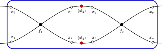
Figure 2.3: Connect variables $x_{\ell}$, $x_{k}$ of $f_{1}$ with variables $x_{s}$, $x_{t}$ of $f_{2}$ both using $(\neq_{2})$.

A binary signature $g$ has the signature vector $g(x_{1},x_{2})=(g_{00},g_{01},g_{10},g_{11})^{T}$, and also $g(x_{2},x_{1})=(g_{00},g_{10},g_{01},g_{11})^{T}$. Without other specification, $g$ denotes $g(x_{1},x_{2})$. Let $f$ be a signature of arity $4$ with the signature matrix $M_{x_{i}x_{j},x_{\ell}x_{k}}(f)$ and $(s,t)$ be a permutation of $(1,2)$. The second gadget construction is as follows. By connecting $x_{\ell}$ with $x_{s}$ and $x_{k}$ with $x_{t}$, both using Disequality $(\neq_{2})$, we get a binary signature with the signature matrix $M_{x_{i}x_{j},x_{k}x_{\ell}}Ng{(x_{s},x_{t})}$ as a matrix product with index $x_{i}x_{j}$ (See Figure 2.4). If $g_{00}=g_{11}$, then $N(g_{00},g_{01},g_{10},g_{11})^{T}=(g_{11},g_{10},g_{01},g_{00})^{T}=(g_{00},g_{10},g_{01},g_{11})^{T}$, and similarly, $N(g_{00},g_{10},g_{01},g_{11})^{T}=(g_{00},g_{01},g_{10},g_{11})^{T}$. Therefore, $M_{x_{i}x_{j},x_{\ell}x_{k}}Ng{(x_{s},x_{t})}=M_{x_{i}x_{j},x_{\ell}x_{k}}g{(x_{t},x_{s})}$, which means that connecting variables $x_{\ell}$, $x_{k}$ of $f$ with, respectively, variables $x_{s}$, $x_{t}$ of $g$ using $N$ is equivalent to connecting them directly without $N$. Hence, in the setting Pl-Holant$(\not=_{2}\mid f,g)$ we can form $M_{x_{i}x_{j},x_{\ell}x_{k}}(f)g{(x_{t},x_{s})}$, which is technically $M_{x_{i}x_{j},x_{\ell}x_{k}}Ng{(x_{s},x_{t})}$, provided that $g_{00}=g_{11}$. Note that for a binary signature $g$, we can rotate it by $180^{\circ}$ without violating planarity, and so both $g(x_{s},x_{t})$ and $g(x_{t},x_{s})$ can be freely used once we get one of them.

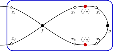
Figure 2.4: Connect variables $x_{\ell}$, $x_{k}$ of $f$ with variables $x_{s}$, $x_{t}$ of $g$ both using $(\neq_{2})$.

A signature $f$ of arity $4$ also has the $2\times 8$ signature matrix

$$M_{x_{1},x_{2}x_{4}x_{3}}(f)=\left[\begin{matrix}f_{0000}&f_{0010}&f_{0001}&f_{0011}&f_{0100}&f_{0110}&f_{0101}&f_{0111}\\ f_{1000}&f_{1010}&f_{1001}&f_{1011}&f_{1100}&f_{1110}&f_{1101}&f_{1111}\end{matrix}\right].$$

Suppose the signature matrix of $g$ is $M_{x_{s},x_{t}}(g)$ and the signature matrix of $f$ is $M_{x_{i},x_{j}x_{\ell}x_{k}}(f)$. Our third gadget construction is as follows. By connecting $x_{t}$ with $x_{i}$ using Disequality $(\neq_{2})$, we get a signature $h$ of arity $4$ with the signature matrix $M_{x_{s},x_{t}}(g)M(\neq_{2})M_{x_{i},x_{j}x_{\ell}x_{k}}(f)$ by matrix product with row index $x_{s}$ and column index $x_{j}x_{\ell}x_{k}$ (See Figure 2.5). We may change this form to a signature matrix with row index $x_{s}x_{j}$ and column index $x_{\ell}x_{k}$.

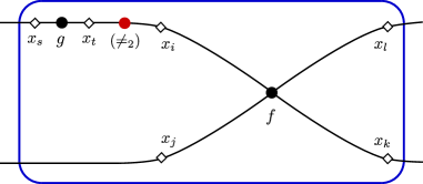
Figure 2.5: Connect variable $x_{t}$ of $g$ with variable $x_{i}$ of $f$ using $(\neq_{2})$.

In particular, if $M_{y_{1},y_{2}}(g)=\left[\begin{smallmatrix}0&1\\ t&0\\ \end{smallmatrix}\right]$, then connecting $y_{2}$ with $x_{1}$ via $(\neq_{2})$ gives

$$M_{y_{1},x_{2}x_{4}x_{3}}(h) =M_{y_{1},y_{2}}(g)M(\neq_{2})M_{x_{1},x_{2}x_{4}x_{3}}(f)$$

$$=\left[\begin{matrix}0&1\\ t&0\\ \end{matrix}\right]\left[\begin{matrix}0&1\\ 1&0\\ \end{matrix}\right]\left[\begin{matrix}f_{0000}&f_{0010}&f_{0001}&f_{0011}&f_{0100}&f_{0110}&f_{0101}&f_{0111}\\ f_{1000}&f_{1010}&f_{1001}&f_{1011}&f_{1100}&f_{1110}&f_{1101}&f_{1111}\end{matrix}\right]$$

$$=\left[\begin{matrix}f_{0000}&f_{0010}&f_{0001}&f_{0011}&f_{0100}&f_{0110}&f_{0101}&f_{0111}\\ tf_{1000}&tf_{1010}&tf_{1001}&tf_{1011}&tf_{1100}&tf_{1110}&tf_{1101}&tf_{1111}\end{matrix}\right].$$

If we rename the variable $y_{1}$ by $x_{1}$, then $M_{x_{1}x_{2},x_{4}x_{3}}(h)=\left[\begin{smallmatrix}f_{0000}&f_{0010}&f_{0001}&f_{0011}\\ f_{0100}&f_{0110}&f_{0101}&f_{0111}\\ tf_{1000}&tf_{1010}&tf_{1001}&tf_{1011}\\ tf_{1100}&tf_{1110}&tf_{1101}&tf_{1111}\end{smallmatrix}\right]$. That is, the new signature has the matrix obtained from multiplying $t$ to the last two rows of $M_{x_{1}x_{2},x_{4}x_{3}}(f)$ corresponding to $x_{1}=1$. Similarly we can modify the last two columns of $M_{x_{1}x_{2},x_{4}x_{3}}(f)$. Given $g=(0,1,t,0)^{T}$, we call the modification from $M_{x_{1}x_{2},x_{4}x_{3}}(f)$ to

$$\left[\begin{matrix}f_{0000}&f_{0010}&f_{0001}&f_{0011}\\ f_{0100}&f_{0110}&f_{0101}&f_{0111}\\ tf_{1000}&tf_{1010}&tf_{1001}&tf_{1011}\\ tf_{1100}&tf_{1110}&tf_{1101}&tf_{1111}\end{matrix}\right]$$

the operation of $t$ scaling on $x_{1}=1$. Similarly we call the modification from $M_{x_{1}x_{2},x_{4}x_{3}}(f)$ to

$$\left[\begin{matrix}f_{0000}&f_{0010}&tf_{0001}&tf_{0011}\\ f_{0100}&f_{0110}&tf_{0101}&tf_{0111}\\ f_{1000}&f_{1010}&tf_{1001}&tf_{1011}\\ f_{1100}&f_{1110}&tf_{1101}&tf_{1111}\end{matrix}\right]$$

the operation of $t$ scaling on $x_{4}=1$.

For any scalar $c\neq 0$ and any set of signatures $\mathcal{F}$, we have $\operatorname{Holant}(\mathcal{F}\cup\{f\})\equiv_{T}\operatorname{Holant}(\mathcal{F}\cup\{cf\})$, and $\operatorname{Pl-Holant}(\mathcal{F}\cup\{f\})\equiv_{T}\operatorname{Pl-Holant}(\mathcal{F}\cup\{cf\})$. Thus a scalar $c\neq 0$ does not change the complexity of a Holant problem. Hence we can normalize any particular nonzero signature entry to be 1.

2.3 Holographic Transformation

To introduce the idea of holographic transformation, it is convenient to consider bipartite graphs. For a general graph, we can always transform it into a bipartite graph while preserving the Holant value, as follows. For each edge in the graph, we replace it by a path of length two. (This operation is called the 2-stretch of the graph and yields the edge-vertex incidence graph.) Each new vertex is assigned the binary Equality signature $=_{2}$. Thus, we have $\operatorname{Holant}\left(=_{2}\mid\mathcal{F}\right)\equiv_{T}\operatorname{Holant}(\mathcal{F})$.

For an invertible $2$-by-$2$ matrix $T\in{\rm GL}_{2}({\mathbb{C}})$ and a signature $f$ of arity $n$, written as a column vector (contravariant tensor) $f\in\mathbb{C}^{2^{n}}$, we denote by $T^{-1}f=(T^{-1})^{\otimes n}f$ the transformed signature. For a signature set $\mathcal{F}$, define $T^{-1}\mathcal{F}=\{T^{-1}f\mid f\in\mathcal{F}\}$ the set of transformed signatures. For signatures written as row vectors (covariant tensors) we define $fT$ and $\mathcal{F}T$ similarly. Whenever we write $T^{-1}f$ or $T^{-1}\mathcal{F}$, we view the signatures as column vectors; similarly for $fT$ or $\mathcal{F}T$ as row vectors. In the special case of the Hadamard matrix $H_{2}=\frac{1}{\sqrt{2}}\left[\begin{smallmatrix}1&1\\ 1&-1\end{smallmatrix}\right]$, we also define $\widehat{\mathcal{F}}=H_{2}\mathcal{F}$. Note that $H_{2}$ is orthogonal. Since constant factors are immaterial, for convenience we sometime drop the factor $\frac{1}{\sqrt{2}}$ when using $H_{2}$.

Let $T\in{\rm GL}_{2}({\mathbb{C}})$. The holographic transformation defined by $T$ is the following operation: given a signature grid $\Omega=(H,\pi)$ of $\operatorname{Holant}\left(\mathcal{F}\mid\mathcal{G}\right)$, for the same bipartite graph $H$, we get a new signature grid $\Omega^{\prime}=(H,\pi^{\prime})$ of $\operatorname{Holant}\left(\mathcal{F}T\mid T^{-1}\mathcal{G}\right)$ by replacing each signature in $\mathcal{F}$ or $\mathcal{G}$ with the corresponding signature in $\mathcal{F}T$ or $T^{-1}\mathcal{G}$. Valiant’s Holant Theorem [50] states that the instances $\Omega$ and $\Omega^{\prime}$ have the same Holant value. This result also holds for planar instances.

Theorem 2.1 ([50]).

For every $T\in{\rm GL}_{2}({\mathbb{C}})$, $\operatorname{Pl-Holant}(\mathcal{F}\mid\mathcal{G})\equiv_{T}\operatorname{Pl-Holant}(\mathcal{F}T\mid T^{-1}\mathcal{G}).$

Definition 2.2.

We say a signature set $\mathcal{F}$ is $\mathscr{C}$-transformable if there exists a $T\in\rm{GL}_{2}(\mathbb{C})$ such that $(0,1,1,0)T^{\otimes 2}\in\mathscr{C}$ and $T^{-1}\mathcal{F}\subseteq\mathscr{C}$.

This definition is important because if $\operatorname{Pl-Holant}(\mathscr{C})$ is tractable, then $\operatorname{Pl-Holant}(\neq_{2}\mid\mathcal{F})$ is tractable for any $\mathscr{C}$-transformable set $\mathcal{F}$.

2.4 Polynomial Interpolation

Polynomial interpolation is a powerful technique to prove #P-hardness for counting problems. We use polynomial interpolation to prove the following lemmas.

Lemma 2.3.

Let $f$ be a 4-ary signature with the signature matrix $M(f)=\left[\begin{smallmatrix}0&0&0&1\\ 0&b&0&0\\ 0&0&b&0\\ 1&0&0&0\\ \end{smallmatrix}\right]$, where $b\neq 0$ is not a root of unity. Let $\chi_{1}$ be a 4-ary signature with the signature matrix $M(\chi_{1})=\left[\begin{smallmatrix}0&0&0&1\\ 0&1&0&0\\ 0&0&1&0\\ 1&0&0&0\\ \end{smallmatrix}\right].$ Then for any signature set $\mathcal{F}$ containing $f$, we have

$$\operatorname{Pl-Holant}(\neq_{2}\mid\mathcal{F}\cup\{\chi_{1}\})\leqslant_{T}\operatorname{Pl-Holant}(\neq_{2}\mid\mathcal{F}).$$

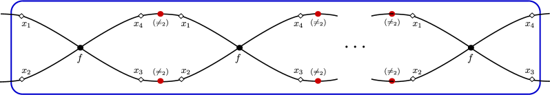
Figure 2.6: A chain of $2s+1$ many copies of $f$ linked by double Disequality $N$

Proof. We construct a series of gadgets $f_{2s+1}$ by a chain of $2s+1$ many copies of $f$ linked by the double Disequality $N$ (See Figure 2.6). Clearly $f_{2s+1}$ has the following signature matrix

$$M(f_{2s+1})=M(f)(NM(f))^{2s}=\left[\begin{matrix}0&0&0&1\\ 0&b^{2s+1}&0&0\\ 0&0&b^{2s+1}&0\\ 1&0&0&0\\ \end{matrix}\right].$$

The matrix $M(f_{2s+1})$ has a good form for polynomial interpolation. Suppose $\chi_{1}$ appears $m$ times in an instance $\Omega$ of $\operatorname{Pl-Holant}(\neq_{2}\mid\mathcal{F}\cup\{\chi_{1}\})$. We replace each appearance of $\chi_{1}$ by a copy of the gadget $f_{2s+1}$ to get an instance $\Omega_{2s+1}$ of $\operatorname{Pl-Holant}(\neq_{2}\mid\mathcal{F}\cup\{f_{2s+1}\})$, which is also an instance of $\operatorname{Pl-Holant}(\neq_{2}\mid\mathcal{F})$. We divide $\Omega_{2s+1}$ into two parts. One part consists of $m$ signatures $f_{2s+1}$ and its signature is represented by $(M(f_{2s+1}))^{\otimes{m}}$. Here we rewrite $(M(f_{2s+1}))^{\otimes{m}}$ as a column vector. The other part is the rest of $\Omega_{2s+1}$ and its signature is represented by $A$ which is a tensor expressed as a row vector. Then, the Holant value of $\Omega_{2s+1}$ is the dot product $\langle A,(M(f_{2s+1}))^{\otimes{m}}\rangle$, which is a summation over $4m$ bits. That is, a sum over all $0,1$ values for the $4m$ edges connecting the two parts. We can stratify all $0,1$ assignments of these $4m$ bits having a nonzero evaluation of a term in Pl-Holant${}_{\Omega_{2s+1}}$ into the following categories:

• There are $i$ many copies of $f_{2s+1}$ receiving inputs $0011$ or $1100$;

• There are $j$ many copies of $f_{2s+1}$ receiving inputs $0110$ or $1001$;

where $i+j=m$.

For any assignment in the category with parameter $(i,j)$, the evaluation of $(M(f_{2s+1}))^{\otimes m}$ is clearly $b^{(2s+1)j}$. Let $a_{ij}$ be the summation of values of the part $A$ over all assignments in the category $(i,j)$. Note that $a_{ij}$ is independent from the value of $s$ since we view the gadget $f_{2s+1}$ as a block. Since $i+j=m$, we can denote $a_{ij}$ by $a_{j}$. Then, we rewrite the dot product summation and get

$$\operatorname{Pl-Holant}_{\Omega_{2s+1}}=\langle A,(M(f_{2s+1}))^{\otimes{m}}\rangle=\sum_{0\leqslant j\leqslant m}a_{j}b^{(2s+1)j}.$$

Under this stratification, the Holant value of $\operatorname{Pl-Holant}(\Omega,\neq_{2}\mid\mathcal{F}\cup\{\chi_{1}\})$ can be represented as

$$\operatorname{Pl-Holant}_{\Omega}=\langle A,(M(\chi_{1}))^{\otimes{m}}\rangle=\sum_{0\leqslant j\leqslant m}a_{j}.$$

Since $b\neq 0$ is not a root of unity, the linear equation system has a nonsingular Vandermonde matrix

$$\left[\begin{matrix}b^{0}&b^{1}&\cdots&b^{m}\\ (b^{3})^{0}&(b^{3})^{1}&\cdots&(b^{3})^{m}\\ \vdots&\vdots&\vdots&\vdots\\ (b^{2m+1})^{0}&(b^{2m+1})^{1}&\cdots&(b^{2m+1})^{m}\\ \end{matrix}\right].$$

By oracle querying the values of $\operatorname{Pl-Holant}_{\Omega_{2s+1}}$, we can solve the coefficients $a_{j}$ in polynomial time and obtain the value of $p(x)=\sum\limits_{0\leqslant j\leqslant m}a_{j}x^{j}$ for any $x$. Let $x=1$, we get $\operatorname{Pl-Holant}_{\Omega}$. Therefore, we have $\operatorname{Pl-Holant}(\neq_{2}\mid\mathcal{F}\cup\{\chi_{1}\})\leqslant_{T}\operatorname{Pl-Holant}(\neq_{2}\mid\mathcal{F}).$∎

Corollary 2.4.

Let $f$ be a 4-ary signature with the signature matrix $M(f)=\left[\begin{smallmatrix}0&0&0&1\\ 0&b&0&0\\ 0&0&b&0\\ -1&0&0&0\\ \end{smallmatrix}\right]$, where $b\neq 0$ is not a root of unity. Let $\chi_{2}$ be a 4-ary signature with the signature matrix $M(\chi_{2})=\left[\begin{smallmatrix}0&0&0&1\\ 0&1&0&0\\ 0&0&1&0\\ -1&0&0&0\\ \end{smallmatrix}\right].$ Then for any signature set $\mathcal{F}$ containing $f$, we have

$$\operatorname{Pl-Holant}(\neq_{2}\mid\mathcal{F}\cup\{\chi_{2}\})\leqslant_{T}\operatorname{Pl-Holant}(\neq_{2}\mid\mathcal{F}).$$

Proof. We still construct a series of gadgets $f_{2s+1}$ by a chain of odd many copies of $f$ linked by the double Disequality $N$. Clearly $f_{2s+1}$ has the following signature matrix

$$M(f_{2s+1})=M(f)(NM(f))^{2s}=\left[\begin{matrix}0&0&0&1\\ 0&b^{2s+1}&0&0\\ 0&0&b^{2s+1}&0\\ -1&0&0&0\\ \end{matrix}\right].$$

Suppose $\chi_{2}$ appears $m$ times in an instance $\Omega$ of $\operatorname{Pl-Holant}(\neq_{2}\mid f\cup\chi_{2})$. We replace each appearance of $\chi_{2}$ by a copy of the gadget $f_{2s+1}$ to get an instance $\Omega_{2s+1}$ of $\operatorname{Pl-Holant}(\neq_{2}\mid\mathcal{F}\cup\{f_{2s+1}\})$. In the same way as in the proof of Lemma 2.3, we divide $\Omega_{2s+1}$ into two parts. One part is represented by $(M(f_{2s+1}))^{\otimes{m}}$ and the other part is represented by $A$. Then, the Holant value of $\Omega_{2s+1}$ is the dot product $\langle A,(M(f_{2s+1}))^{\otimes{m}}\rangle$. We can stratify all $0,1$ assignments of these $4m$ bits having a nonzero evaluation of a term in Pl-Holant${}_{\Omega_{2s+1}}$ into the following categories:

• There are $i$ many copies of $f_{2s+1}$ receiving inputs $0011$;

• There are $j$ many copies of $f_{2s+1}$ receiving inputs $0110$ or $1001$;

• There are $k$ many copies of $f_{2s+1}$ receiving inputs $1100$;

where $i+j+k=m$.

For any assignment in those categories with parameters $(i,j,k)$ where $k\equiv 0\pmod{2}$, the evaluation of $(M(f_{2s+1}))^{\otimes m}$ is clearly $(-1)^{k}b^{(2s+1)j}=b^{(2s+1)j}$. And for any assignment in those categories with parameters $(i,j,k)$ where $k\equiv 1\pmod{2}$, the evaluation of $(M(f_{2s+1}))^{\otimes m}$ is clearly $(-1)^{k}b^{(2s+1)j}=-b^{(2s+1)j}$. Since $i+j+k=m$, the index $i$ is determined by $j$ and $k$. Let $a_{j0}$ be the summation of values of the part $A$ over all assignments in those categories $(i,j,k)$ where $k\equiv 0\pmod{2}$, and $a_{j1}$ be the summation of values of the part $A$ over all assignments in those categories $(i,j,k)$ where $k\equiv 1\pmod{2}$. Note that $a_{j0}$ and $a_{j1}$ are independent from the value of $s$. Let $a_{j}=a_{j0}-a_{j1}$. Then, we rewrite the dot product summation and get

$$\operatorname{Pl-Holant}_{\Omega_{2s+1}}=\langle A,(M(f_{2s+1}))^{\otimes{m}}\rangle=\sum_{0\leqslant j\leqslant m}(a_{j0}b^{(2s+1)j}-a_{j1}b^{(2s+1)j})=\sum_{0\leqslant j\leqslant m}a_{j}b^{(2s+1)j}.$$

Under this stratification, the Holant value of $\operatorname{Pl-Holant}\left(\Omega;\neq_{2}\mid f\cup\chi_{2}\right)$ can be represented as

$$\operatorname{Pl-Holant}_{\Omega}=\langle A,(M(\chi_{2}))^{\otimes{m}}\rangle=\sum_{0\leqslant j\leqslant m}(a_{j0}-a_{j1})=\sum_{0\leqslant j\leqslant m}a_{j}.$$

Since $b\neq 0$ is not a root of unity, the Vandermonde coefficient matrix has full rank. Hence we can solve for all the values $a_{j}$ in polynomial time and obtain the value $\sum\limits_{0\leqslant j\leqslant m}a_{j}$, and so we get $\operatorname{Pl-Holant}_{\Omega}$. Therefore, we have $\operatorname{Pl-Holant}(\neq_{2}\mid\mathcal{F}\cup\{\chi_{2}\})\leqslant_{T}\operatorname{Pl-Holant}(\neq_{2}\mid\mathcal{F}).$∎

Lemma 2.5.

Let $g=(0,1,t,0)^{T}$ be a binary signature, where $t\neq 0$ is not a root of unity. Then for any binary signature $g^{\prime}$ of the form $(0,1,t^{\prime},0)^{T}$ and any signature set $\mathcal{F}$ containing $g$, we have

$$\operatorname{Pl-Holant}\left(\neq_{2}\mid\mathcal{F}\cup\{g^{\prime}\}\right)\leqslant_{T}\operatorname{Pl-Holant}\left(\neq_{2}\mid\mathcal{F}\right).$$

Inductively, for any finite signature set $\mathcal{B}$ consisting of binary signatures of the form $(0,1,t^{\prime},0)^{T}$ and any signature set $\mathcal{F}$ containing $g$, we have

$$\operatorname{Pl-Holant}\left(\neq_{2}\mid\mathcal{F}\cup\mathcal{B}\right)\leqslant_{T}\operatorname{Pl-Holant}\left(\neq_{2}\mid\mathcal{F}\right).$$

Proof. Note that $M(g)=\left[\begin{smallmatrix}0&1\\ t&0\\ \end{smallmatrix}\right]$. Connecting the variable $x_{2}$ of a copy of $g$ with the variable $x_{1}$ of another copy of $g$ using $(\neq_{2})$, we get a signature $g_{2}$ with the signature matrix

$$M(g_{2})=M_{x_{1},x_{2}}(g)M(\neq_{2})M_{x_{1},x_{2}}(g)=\left[\begin{matrix}0&1\\ t&0\\ \end{matrix}\right]\left[\begin{matrix}0&1\\ 1&0\\ \end{matrix}\right]\left[\begin{matrix}0&1\\ t&0\\ \end{matrix}\right]=\left[\begin{matrix}0&1\\ t^{2}&0\\ \end{matrix}\right].$$

That is, $g_{2}=(0,1,t^{2},0)^{T}.$ Recursively, we can construct $g_{s}=(0,1,t^{s},0)^{T}$ for $s\geq 1$. Here, $g_{1}$ denotes $g$. Given an instance $\Omega^{\prime}$ of $\operatorname{Pl-Holant}\left(\neq_{2}\mid\mathcal{F}\cup\{g^{\prime}\}\right)$, in the same way as in the proof of Lemma 2.3, we can replace each appearance of $g^{\prime}$ by $g_{s}$ and get an instance $\Omega_{s}$ of $\operatorname{Pl-Holant}\left(\neq_{2}\mid\mathcal{F}\right)$. Similarly, the Holant value of $\Omega_{s}$ can be represented as

$$\operatorname{Pl-Holant}_{\Omega_{s}}=\sum_{0\leqslant j\leqslant m}a_{j}(t^{s})^{j},$$

while the Holant value of $\Omega^{\prime}$ can be represented as

$$\operatorname{Pl-Holant}_{\Omega^{\prime}}=\sum_{0\leqslant j\leqslant m}a_{j}(t^{\prime})^{j}.$$

Since $t\neq 0$ is not a root of unity, all $t^{s}$ are distinct, and so the Vandermonde coefficient matrix has full rank. Hence, we can solve for all $a_{j}$, and then compute $\sum\limits_{0\leqslant j\leqslant m}a_{j}(t^{\prime})^{j}$. So we get $\operatorname{Pl-Holant}_{\Omega^{\prime}}$. Therefore, we have $\operatorname{Pl-Holant}(\neq_{2}\mid\mathcal{F}\cup\{g^{\prime}\})\leqslant_{T}\operatorname{Pl-Holant}(\neq_{2}\mid\mathcal{F}).$ The second part of this lemma follows directly by the first part. ∎

Remark: Note that the reason why the interpolation can succeed is that we can construct polynomially many binary signatures $g_{s}$ of the form $(0,1,t_{s},0)^{T}$, where all $t_{s}$ are distinct such that the Vandermonde coefficient matrix has full rank. According to this, we have the following corollary.

Corollary 2.6.

Given a signature set $\mathcal{F}$, if we can use $\mathcal{F}$ to construct polynomially many distinct binary signatures $g_{s}=(0,1,t_{s},0)^{T}$, then for any finite signature set $\mathcal{B}$ consisting of binary signatures of the form $(0,1,t^{\prime},0)^{T}$, we have

$$\operatorname{Pl-Holant}\left(\neq_{2}\mid\mathcal{F}\cup\mathcal{B}\right)\leqslant_{T}\operatorname{Pl-Holant}\left(\neq_{2}\mid\mathcal{F}\right).$$

In Lemma 6.4, we will show how to construct polynomially many distinct binary signatures $g_{s}=(0,1,t_{s},0)^{T}$ using Möbius transformations [2]. A Möbius transformation of the extended complex plane $\widehat{\mathbb{C}}=\mathbb{C}\cup\{\infty\}$, the complex plane plus a point at infinity, is a rational function of the form $\mathfrak{z}\mapsto\dfrac{a\mathfrak{z}+b}{c\mathfrak{z}+d}$ of a complex variable $\mathfrak{z}$, where the coefficients $a,b,c,d$ are complex numbers satisfying $\det\left[\begin{smallmatrix}a&b\\ c&d\\ \end{smallmatrix}\right]=ad-bc\neq 0$. It is a bijective conformal map. In particular, a Möbius transformation mapping the unit circle $S^{1}=\{z\mid|z|=1\}$ to itself is of the form $\varphi(\mathfrak{z})=e^{\mathfrak{i}\theta}\dfrac{(\mathfrak{z}+\alpha)}{1+\bar{\alpha}\mathfrak{z}}$ denoted by $\mathcal{M}(\alpha,e^{\mathfrak{i}\theta})$, where $|\alpha|\neq 1$, or $\varphi(\mathfrak{z})=e^{\mathfrak{i}\theta}/{\mathfrak{z}}$. When $|\alpha|<1$, it maps the interior of $S^{1}$ to the interior, while when $|\alpha|>1$, it maps the interior of $S^{1}$ to the exterior. A Möbius transformation is completely determined by its values on any $3$ distinct points of $\widehat{\mathbb{C}}$.

An interpolation proof based on a lattice structure will be given in Lemma 6.1, where the following lemma is used.

Lemma 2.7.

[18] Suppose $\alpha,\beta\in\mathbb{C}-\{0\}$, and the lattice $L=\{(j,k)\in\mathbb{Z}^{2}\mid\alpha^{j}\beta^{k}=1\}$ has the form $L=\{(ns,nt)\mid n\in\mathbb{Z}\}$, where $s,t\in\mathbb{Z}$ and $(s,t)\neq(0,0)$. Let $\phi$ and $\psi$ be any numbers satisfying $\phi^{s}\psi^{t}=1$. If we are given the values $N_{\ell}=\sum_{j,k\geq 0,\leavevmode\nobreak\ j+k\leq m}(\alpha^{j}\beta^{k})^{\ell}x_{j,k}$ for ${\ell}=1,2,\ldots{m+2\choose 2}$, then we can compute $\sum_{j,k\geq 0,\leavevmode\nobreak\ j+k\leq m}\phi^{j}\psi^{k}x_{j,k}$ in polynomial time.

2.5 Tractable Signature Sets

We give some sets of signatures that are known to define tractable counting problems. These are called tractable signatures. There are three families: affine signatures, product-type signatures, and matchgate signatures  [14].

Affine Signatures

Definition 2.8.

For a signature $f$ of arity $n$, the support of $f$ is

$$\operatorname{supp}(f)=\{(x_{1},x_{2},\ldots,x_{n})\in\mathbb{Z}_{2}^{n}\mid f(x_{1},x_{2},\ldots,x_{n})\neq 0\}.$$

Definition 2.9.

A signature $f(x_{1},\ldots,x_{n})$ of arity $n$ is affine if it has the form

$$\lambda\cdot\chi_{AX=0}\cdot{\mathfrak{i}}^{Q(X)},$$

where $\lambda\in\mathbb{C}$, $X=(x_{1},x_{2},\dotsc,x_{n},1)$, $A$ is a matrix over $\mathbb{Z}_{2}$, $Q(x_{1},x_{2},\ldots,x_{n})\in\mathbb{Z}_{4}[x_{1},x_{2},\ldots,x_{n}]$ is a quadratic (total degree at most 2) multilinear polynomial with the additional requirement that the coefficients of all cross terms are even, i.e., $Q$ has the form

$$Q(x_{1},x_{2},\ldots,x_{n})=a_{0}+\displaystyle\sum_{k=1}^{n}a_{k}x_{k}+\displaystyle\sum_{1\leq i<j\leq n}2b_{ij}x_{i}x_{j},$$

and $\chi$ is a 0-1 indicator function such that $\chi_{AX=0}$ is $1$ iff $AX=0$. We use $\mathscr{A}$ to denote the set of all affine signatures.

The following two lemmas follow directly from the definition.

Lemma 2.10.

Let $g$ be a binary signature with support of size $4$. Then, $g\in\mathscr{A}$ iff $g$ has the signature matrix $M(g)=\lambda\left[\begin{smallmatrix}\mathfrak{i}^{a}&\mathfrak{i}^{b}\\ \mathfrak{i}^{c}&\mathfrak{i}^{d}\end{smallmatrix}\right]$, for some nonzero $\lambda\in\mathbb{C}$, $a,b,c,d\in\mathbb{N}$ and $a+b+c+d\equiv 0\pmod{2}$.

Lemma 2.11.

Let $h$ be a unary signature with support of size $2$. Then, $h\in\mathscr{A}$ iff $h$ has the form $M(h)=\lambda\left[\begin{matrix}\mathfrak{i}^{a}&\mathfrak{i}^{b}\end{matrix}\right]$, for some nonzero $\lambda\in\mathbb{C}$, and $a,b\in\mathbb{N}$.

Product-Type Signatures

Definition 2.12.

A signature on a set of variables $X$ is of product type if it can be expressed as a product of unary functions, binary equality functions $([1,0,1])$, and binary disequality functions $([0,1,0])$, each on one or two variables of $X$. We use $\mathscr{P}$ to denote the set of product-type functions.

Note that the variables of the functions in the product need not be distinct. E.g., let $f(x,y,z)$ be listed as $\left[\begin{smallmatrix}f_{000}&f_{001}&f_{010}&f_{011}\\ f_{100}&f_{101}&f_{110}&f_{111}\end{smallmatrix}\right]=\left[\begin{smallmatrix}0&a&0&0\\ 0&0&b&0\end{smallmatrix}\right]$. $f$ is the product of $(=_{2})(x,y)$, $(\neq_{2})(x,z)$ and $[a,b](x)$. Let $g$ be $\left[\begin{smallmatrix} g_{00}&g_{01}\\  g_{10}&g_{11}\end{smallmatrix}\right]=\left[\begin{smallmatrix}0&c\\ d&0\end{smallmatrix}\right]$, and $h(x,y,z,w)=f(x,y,z)g(z,w)$, sharing a variable $z$. Then $f,g,h\in\mathscr{P}$.

The following theorem is known [22], since $(\neq_{2})\in\mathscr{A}\cap\mathscr{P}$.

Theorem 2.13.

Let $\mathcal{F}$ be any set of complex-valued signatures in Boolean variables. If $\mathcal{F}\subseteq\mathscr{A}$ or $\mathcal{F}\subseteq\mathscr{P}$, then $\operatorname{Holant}(\neq_{2}\mid\mathcal{F})$ is tractable.

Matchgate Signatures

Matchgates were introduced by Valiant [49, 48] to give polynomial-time algorithms for a collection of counting problems over planar graphs. As the name suggests, problems expressible by matchgates can be reduced to computing a weighted sum of perfect matchings. The latter problem is tractable over planar graphs by Kasteleyn’s algorithm [34], a.k.a. the FKT algorithm [46, 35]. These counting problems are naturally expressed in the Holant framework using matchgate signatures. We use $\mathscr{M}$ to denote the set of all matchgate signatures; thus $\operatorname{Pl-Holant}(\mathscr{M})$ is tractable, as well as $\operatorname{Pl-Holant}(\neq_{2}\mid\mathscr{M})$.

The parity of a signature is even (resp. odd) if its support is on entries of even (resp. odd) Hamming weight. We say a signature satisfies the even (resp. odd) Parity Condition if all entries of odd (resp. even) weight are zero. For signatures of arity at most $4$, the matchgate signatures are characterized by the following lemma.

Lemma 2.14 ([48, 10]).

If $f$ has arity $\leqslant 3$, then $f\in\mathscr{M}$ iff $f$ satisfies the Parity Condition.

If $f$ has arity 4 and $f$ satisfies the even Parity Condition, i.e.,

$$M_{x_{1}x_{2},x_{4}x_{3}}(f)=\begin{bmatrix}f_{0000}&0&0&f_{0011}\\ 0&f_{0110}&f_{0101}&0\\ 0&f_{1010}&f_{1001}&0\\ f_{1100}&0&0&f_{1111}\\ \end{bmatrix},$$

then $f\in\mathscr{M}$ iff

$$\det M_{\rm{Out}}(f)=\det M_{\rm{In}}(f).$$

By this matchgate identity, we have the following corollary.

Corollary 2.15.

Given a signature $f$ of arity $4$, two $2$-by-$2$ matrices $D_{\lambda}=\left[\begin{smallmatrix}1&0\\ 0&\lambda\\ \end{smallmatrix}\right](\lambda\neq 0)$ and $M(\neq_{2})=\left[\begin{smallmatrix}0&1\\ 1&0\\ \end{smallmatrix}\right]$, if $f\in\mathscr{M}$, then $D_{\lambda}f$ and $M(\neq_{2})f\in\mathscr{M}$.

Proof. Since $f\in\mathscr{M}$, by Lemma 2.14 we know $f$ satisfies the Parity Condition. We only consider that $f$ satisfies even parity. The proof for $f$ satisfying odd parity is similar and we omitted it here. Suppose $f$ has the signature matrix $M(f)=\left[\begin{smallmatrix}d&0&0&a\\ 0&b&c&0\\ 0&z&y&0\\ x&0&0&w\\ \end{smallmatrix}\right]$. Then, we have $M(D_{\lambda}f)=\left[\begin{smallmatrix}d&0&0&\lambda^{2}a\\ 0&\lambda^{2}b&\lambda^{2}c&0\\ 0&\lambda^{2}z&\lambda^{2}y&0\\ \lambda^{2}x&0&0&\lambda^{4}w\\ \end{smallmatrix}\right]$ and $M(M(\neq_{2})f)=\left[\begin{smallmatrix}w&0&0&x\\ 0&y&z&0\\ 0&c&b&0\\ a&0&0&d\\ \end{smallmatrix}\right]$. Clearly, $D_{\lambda}f$ and $M(\neq_{2})f$ also satisfy even parity. Moreover, we have

$$\det M_{\rm{Out}}(D_{\lambda}f)=\lambda^{4}\det M_{\rm{Out}}(f),\det M_{\rm{In}}(D_{\lambda}f)=\lambda^{4}\det M_{\rm{In}}(f),$$

and

$$\det M_{\rm{Out}}(M(\neq_{2})f)=\det M_{\rm{Out}}(f),\det M_{\rm{In}}(M(\neq_{2})f)=\det M_{\rm{In}}(f).$$

Since $\det M_{\rm{Out}}(f)=\det M_{\rm{In}}(f),$ we have

$$\det M_{\rm{Out}}(D_{\lambda}f)=\det M_{\rm{In}}(D_{\lambda}f),\text{ and }\det M_{\rm{Out}}(M(\neq_{2})f)=\det M_{\rm{In}}(M(\neq_{2})f).$$

That is, $D_{\lambda}f$ and $M(\neq_{2})f\in\mathscr{M}.$ ∎

Holographic transformations extend the reach of the FKT algorithm further, as stated below. By Definition 2.2, a signature set $\mathcal{F}$ is $\mathscr{M}$-transformable if there exists a $T\in\rm{GL}_{2}(\mathbb{C})$ such that $(0,1,1,0)T^{\otimes 2}\in\mathscr{M}$ and $T^{-1}\mathcal{F}\subseteq\mathscr{M}$.

Theorem 2.16.

Let $\mathcal{F}$ be any set of complex-valued signatures in Boolean variables. If $\mathcal{F}$ is $\mathscr{M}$-transformable, then $\operatorname{Pl-Holant}(\neq_{2}\mid\mathcal{F})$ is tractable.

We will show that for the six-vertex model, $\mathscr{M}$-transformable signatures are exactly characterized by $\mathscr{M}$ and $\widehat{\mathscr{M}}$. Recall the signature class $\widehat{\mathscr{M}}=H_{2}\mathscr{M}$, where $H_{2}=\frac{1}{\sqrt{2}}\left[\begin{smallmatrix}1&1\\ 1&-1\end{smallmatrix}\right]$. We first give the following simple lemma.

Lemma 2.17.

For any signature $f$ with the signature matrix $M(f)=\left[\begin{smallmatrix}0&0&0&a\\ 0&b&c&0\\ 0&z&y&0\\ x&0&0&0\end{smallmatrix}\right]$, and a $2$-by-$2$ matrix $D_{\lambda}=\left[\begin{smallmatrix}1&0\\ 0&\lambda\\ \end{smallmatrix}\right]$, where $\lambda\neq 0$, we have $f\in\mathscr{\widehat{M}}$ iff $(D_{\lambda})^{\otimes 4}f\in\mathscr{\widehat{M}}$.

Proof. Note that $M((D_{\lambda})^{\otimes 4}f)=\left[\begin{smallmatrix}0&0&0&\lambda^{2}a\\ 0&\lambda^{2}b&\lambda^{2}c&0\\ 0&\lambda^{2}z&\lambda^{2}y&0\\ \lambda^{2}x&0&0&0\end{smallmatrix}\right]=\lambda^{2}M(f).$ That is, $(D_{\lambda})^{\otimes 4}f=\lambda^{2}f$. Thus, $f\in\mathscr{\widehat{M}}$ is equivalent to $(D_{\lambda})^{\otimes 4}f=\lambda^{2}f\in\mathscr{\widehat{M}}$. ∎

Lemma 2.18.

A signature $f$ with the signature matrix $M(f)=\left[\begin{smallmatrix}0&0&0&a\\ 0&b&c&0\\ 0&z&y&0\\ x&0&0&0\end{smallmatrix}\right]$ is $\mathscr{M}$-transformable iff $f\in\mathscr{\widehat{M}}$.

Proof. The reverse direction is obvious, since $(\not=_{2})I^{\otimes 2}\in\mathscr{{M}}$, and $(\not=_{2})H_{2}^{\otimes 2}\in\mathscr{{M}}$.

Suppose $f$ is $\mathscr{M}$-transformable. By definition, there is $T\in\rm{GL}_{2}(\mathbb{C})$ such that

$$(0,1,1,0)T^{\otimes 2}\in\mathscr{M}\leavevmode\nobreak\ \leavevmode\nobreak\ \leavevmode\nobreak\ \mbox{and}\leavevmode\nobreak\ \leavevmode\nobreak\ \leavevmode\nobreak\ (T^{-1})^{\otimes 4}f\in\mathscr{M}.$$

Let $T=\left[\begin{smallmatrix}\lambda&\mu\\ \nu&\xi\\ \end{smallmatrix}\right]$. We have

$$(0,1,1,0)T^{\otimes 2}=(2\lambda\nu,\lambda\xi+\mu\nu,\lambda\xi+\mu\nu,2\mu\xi)\in\mathscr{M}.$$

By Lemma 2.14, we have $\lambda\nu=\mu\xi=0$ or $\lambda\xi+\mu\nu=0$.

If $\lambda\nu=\mu\xi=0$, since $T\in\rm{GL}_{2}(\mathbb{C})$, we have $\mu=\nu=0$ while $\lambda,\xi\neq 0$, or $\lambda=\xi=0$ while $\mu,\nu\neq 0$. That is, $T=\left[\begin{smallmatrix}\lambda&0\\ 0&\xi\\ \end{smallmatrix}\right]$ $(\lambda,\xi\neq 0)$, or $T=\left[\begin{smallmatrix}0&\mu\\ \nu&0\\ \end{smallmatrix}\right]$ $(\mu,\nu\neq 0)$. By normalization, we may assume $\lambda=1$ or $\mu=1$. That is,

$$T=\left[\begin{matrix}1&0\\ 0&\xi\\ \end{matrix}\right](\xi\neq 0),\text{ or }T=\left[\begin{matrix}0&1\\ \nu&0\\ \end{matrix}\right]=\left[\begin{matrix}1&0\\ 0&\nu\\ \end{matrix}\right]\left[\begin{matrix}0&1\\ 1&0\\ \end{matrix}\right](\nu\neq 0).$$

For any $\alpha\neq 0$, we use $D_{\alpha}$ to denote the matrix $\left[\begin{smallmatrix}1&0\\ 0&\alpha\\ \end{smallmatrix}\right]$ and we know $D_{\alpha}^{-1}=D_{1/\alpha}.$ Then, $T=D_{\xi}$ or $T=D_{\nu}M(\neq_{2})$. By Corollary 2.15, we know $f\in\mathscr{M}$ given $T^{-1}f\in\mathscr{M}$.

Otherwise, $\lambda\xi+\mu\nu=0$. Since $T\in\rm{GL}_{2}(\mathbb{C})$, we know $\det T=\lambda\xi-\mu\nu\neq 0$. Thus, $\lambda\xi\mu\nu\neq 0$. By normalization, we may assume $\lambda=1$ and hence, $\xi=-\mu\nu$. That is

$$T=\left[\begin{matrix}1&\mu\\ \nu&-\mu\nu\\ \end{matrix}\right]=\left[\begin{matrix}1&0\\ 0&\nu\\ \end{matrix}\right]\left[\begin{matrix}1&1\\ 1&-1\\ \end{matrix}\right]\left[\begin{matrix}1&0\\ 0&\mu\\ \end{matrix}\right]=D_{\nu}H_{2}D_{\mu}.$$

Hence, we have $T^{-1}=\frac{1}{2}D_{1/\mu}H_{2}D_{1/\nu}$ and we know $D_{1/\mu}H_{2}D_{1/\nu}f\in\mathscr{M}$. We have $D_{\mu}\mathscr{M}=\mathscr{M}$. Hence $H_{2}D_{1/\nu}f\in\mathscr{M}$. Thus, we have

$$D_{1/\nu}f\in\widehat{\mathscr{M}}.$$

By Lemma 2.17, we have $f\in\widehat{\mathscr{M}}$ given $D_{1/\nu}^{\otimes 4}f\in\widehat{\mathscr{M}}$. ∎

For signatures of special forms, we give the following three characterizations of $\widehat{\mathscr{M}}$. They follow directly from the definition.

Lemma 2.19.

A binary signature $g$ with the signature matrix $M(g)=\left[\begin{smallmatrix}g_{00}&g_{01}\\ g_{10}&g_{11}\\ \end{smallmatrix}\right]$ is in $\mathscr{\widehat{M}}$ iff $g_{00}=\epsilon g_{11}$ and $g_{01}=\epsilon g_{10}$, where $\epsilon=\pm 1$.

Lemma 2.20.

A signature $f$ with the signature matrix $M(f)=\left[\begin{smallmatrix}0&0&0&0\\ 0&b&c&0\\ 0&z&y&0\\ 0&0&0&0\end{smallmatrix}\right]$ is in $\mathscr{\widehat{M}}$ iff $b=\epsilon y$ and $c=\epsilon z$, where $\epsilon=\pm 1$.

Lemma 2.21.

If $f$ has the signature matrix $M(f)=\left[\begin{smallmatrix}0&0&0&a\\ 0&b&0&0\\ 0&0&y&0\\ x&0&0&0\end{smallmatrix}\right]$, where $abxy\neq 0$, then $f\notin\mathscr{\widehat{M}}$.

2.6 Known Dichotomies and Hardness Results

Definition 2.22.

A 4-ary signature is non-singular redundant iff in one of its four $4\times 4$ signature matrices, the middle two rows are identical and the middle two columns are identical, and the determinant

$$\det\left[\begin{matrix}f_{0000}&f_{0010}&f_{0011}\\ f_{0100}&f_{0110}&f_{0111}\\ f_{1100}&f_{1110}&f_{1111}\end{matrix}\right]\not=0.$$

Theorem 2.23.

[19] If $f$ is a non-singular redundant signature, then $\operatorname{Pl-Holant}(\neq_{2}|f)$ is ${\#\rm{P}}$-hard.

Theorem 2.24.

[38] Let $G$ be a connected plane graph and $\mathcal{EO}(H)$ be the set of all Eulerian orientations of the medial graph $H=H(G)$ which is a 4-regular planar graph. Then

$$\sum_{O\in\mathcal{EO}(H)}2^{\beta(O)}=2T(G;3,3),$$

where $T$ is the Tutte polynomial, and $\beta(O)$ is the number of saddle vertices in the orientation $O$, i.e., vertices in which the edges are oriented “in, out, in, out” in cyclic order.

Remark: Note that $\sum_{O\in\mathcal{EO}(H)}2^{\beta(O)}$ can be expressed as Pl-Holant$(\neq_{2}\mid f)$ on $H$, where $f$ has the signature matrix $M(f)=\left[\begin{smallmatrix}0&0&0&1\\ 0&1&2&0\\ 0&2&1&0\\ 1&0&0&0\end{smallmatrix}\right]$. Therefore, Pl-Holant$(\neq_{2}\mid f)$ is ${\#\rm{P}}$-hard.

Theorem 2.25.

[14] Let $\mathcal{F}$ be any set of complex-valued signatures in Boolean variables. Then $\operatorname{Pl-\#CSP}(\mathcal{F})$ is ${\#\rm{P}}$-hard unless $\mathcal{F}\subseteq\mathscr{A}$, $\mathcal{F}\subseteq\mathscr{P}$, or $\mathcal{F}\subseteq\widehat{\mathscr{M}}$, in which case the problem is computable in polynomial time. If $\mathcal{F}\subseteq\mathscr{A}$ or $\mathcal{F}\subseteq\mathscr{P}$, then #CSP$(\mathcal{F})$ is computable in polynomial time without planarity; otherwise #CSP$(\mathcal{F})$ is ${\#\rm{P}}$-hard.

Theorem 2.26.

[18] Let $f$ be a 4-ary signature with the signature matrix $M(f)=\left[\begin{smallmatrix}0&0&0&a\\ 0&b&c&0\\ 0&z&y&0\\ x&0&0&0\end{smallmatrix}\right]$, then $\operatorname{Holant}\left(\neq_{2}\mid f\right)$ is #P-hard except for the following cases:

• $f\in\mathscr{P}$;

• $f\in\mathscr{A}$;

• there is a zero in each pair $(a,x),(b,y),(c,z)$;

in which cases $\operatorname{Holant}\left(\neq_{2}\mid f\right)$ is computable in polynomial time.

3 Main Theorem, Proof Outline and Sample Problems

Theorem 3.1.

Let $f$ be a signature with the signature matrix $M(f)=\left[\begin{smallmatrix}0&0&0&a\\ 0&b&c&0\\ 0&z&y&0\\ x&0&0&0\end{smallmatrix}\right]$, where $a,b,c,x,y,z\in\mathbb{C}$. Then $\operatorname{Pl-Holant}(\neq_{2}\mid f)$ is polynomial time computable in the following cases, and #P-hard otherwise:

1. $f\in\mathscr{P}$ or $\mathscr{A}$;

2. There is a zero in each pair $(a,x)$, $(b,y)$, $(c,z)$;

3. $f\in\mathscr{M}$ or $\widehat{\mathscr{M}}$;

4. $c=z=0$ and

   • $(ax)^{2}=(by)^{2}$, or

   • $x=a\mathfrak{i}^{\alpha},b=a\sqrt{\mathfrak{i}}^{\beta}$, and $y=a\sqrt{\mathfrak{i}}^{\gamma}$, where $\alpha,\beta,\gamma\in\mathbb{N}$, and $\beta\equiv\gamma\pmod{2};$

If $f$ satisfies condition 1 or 2, then $\operatorname{Holant}(\neq_{2}\mid f)$ is computable in polynomial time without the planarity restriction; otherwise (the non-planar) $\operatorname{Holant}(\neq_{2}\mid f)$ is #P-hard.

Let ${\sf N}$ be the number of zeros among $a,b,c,x,y,z$. The following division of all cases into Cases I, II, III and IV may not appear to be the most obvious, but it is done to simplify the organization of the proof. We define:

Case I: There is exactly one zero in each pair.

Case II: There is a zero pair.

Case III: ${\sf N}=2$ and having no zero pair, or ${\sf N}=1$ and the zero is in an outer pair.

Case IV: ${\sf N}=1$ and the zero is in an inner pair, or ${\sf N}=0$.

Cases I, II, III and IV are clearly disjoint. To see that they cover all cases, note that if ${\sf N}\geqslant 3$, then either there is a zero pair (in Case II), or ${\sf N}=3$ and each pair has exactly one zero (in Case I). If ${\sf N}=2$, then either it has a zero pair (in Case II), or it has no zero pair (in Case III). If ${\sf N}=1$, then either the single zero is in an outer pair (in Case III), or the single zero is in an inner pair (Case IV). If ${\sf N}=0$ it is in Case IV.

Also note that if ${\sf N}=2$ and it has no zero pair, then the two zeros are in different pairs, which implies that there is a zero in an outer pair. So in Case III, there is a zero in an outer pair regardless ${\sf N}=1$ or ${\sf N}=2$. In Case III an outer pair has exactly one zero, and the other two pairs together have at most one zero.

In Case II, depending on whether the zero pair is inner or outer we have two different connections to #CSP. A previously established connection to #CSP (see [18]) can be adapted in the planar setting to handle the case with a zero outer pair. This connection is a local transformation, and we observe that it preserves planarity. A significantly more involved non-local connection to #CSP is discovered in this paper when the inner pair is zero (and no outer pair is zero). We show that by the support structure of the signature we can define a set of circuits, which forms a partition of the edge set. There are exactly two valid configurations along each such circuit, corresponding to its two cyclic orientations. These circuits may intersect in complicated ways, including self-intersections. But we can define a #CSP problem, where the variables are these circuits, and their edge functions exactly account for the intersections. We show that $\operatorname{Pl-Holant}(\neq_{2}\mid f)$ is equivalent to these #CSP problems, which are non-planar in general. However, crucially, because $\operatorname{Pl-Holant}(\neq_{2}\mid f)$ is planar, every two such circuits must intersect an even number of times. Due to the planarity of $\operatorname{Pl-Holant}(\neq_{2}\mid f)$ we can exactly carve out a new class of tractable problems via this non-local #CSP connection, by the kind of constraint functions they produce in the #CSP problems.

For the proof of #P-hardness in this paper, one particularly difficult case is in Lemma 6.4. This is where we introduce Möbius transformations to prove dichotomy theorems for counting problems. In this case, all constructible binary signatures correspond to points on the unit circle $S^{1}$, and any iteration of the construction amounts to mapping this point by a Möbius transformation which preserves $S^{1}$.

The following is an outline on how Case I to Case IV are handled.

1. There is exactly one zero in each pair. In this case, $\operatorname{Holant}\left(\neq_{2}\mid f\right)$ is tractable, proved in [18].

2. There is a zero pair:

   1. An outer pair $(a,x)$ or $(b,y)$ is a zero pair. We prove that $\operatorname{Pl-Holant}(\neq_{2}\mid f)$ is tractable if $f\in\mathscr{P},\mathscr{A},\mathscr{M}$ or $\widehat{\mathscr{M}}$, and is #P-hard otherwise.

      In this Case ii@.1, we can rotate the signature $f$ such that the matrix $M_{\text{Out}}(f)$ is the zero matrix. Let $M(\widetilde{f}_{\rm{In}})=M_{\rm{In}}(f)\left[\begin{smallmatrix}0&1\\ 1&0\\ \end{smallmatrix}\right]$. We reduce Pl-#CSP$(\widetilde{f}_{\rm In})$ to $\operatorname{Pl-Holant}\left(\neq_{2}\mid f\right)$ via a local replacement (Lemma 4.2). We apply the dichotomy of Pl-#CSP to get #P-hardness (Theorem 4.3). Tractability of $\operatorname{Pl-Holant}\left(\neq_{2}\mid f\right)$ follows from known tractable signatures.

   2. The inner pair $(c,z)$ is a zero pair and no outer pair is a zero pair. We prove that $\operatorname{Pl-Holant}(\neq_{2}\mid f)$ is #P-hard unless $f$ satisfies condition 4, in which case it is tractable.

      This is the non-local reduction described above. The tractable condition 4 is previously unknown. (Curiously, in Case ii@.2, condition 4 subsumes $f\in\mathscr{M}$.)

3. 1. There are exactly two zeros and they are in different pairs;

   2. There is exactly one zero and it is in an outer pair.

   We prove that $\operatorname{Pl-Holant}(\neq_{2}\mid f)$ is #P-hard unless $f\in\mathscr{M}$, in which case it is tractable.

   In Case III, there exists an outer pair which contains a single zero. By connecting two copies of the signature $f$, we can construct a $4$-ary signature $f_{1}$ such that one outer pair is a zero pair. When $f\notin\mathscr{M}$, we can realize a signature $M(g)=\left[\begin{smallmatrix}0&0&0&0\\ 0&0&1&0\\ 0&1&0&0\\ 0&0&0&0\\ \end{smallmatrix}\right]$ by interpolation using $f_{1}$ (Lemma 5.1). This $g$ can help us “extract” the inner matrix of $M(f)$. By connecting $f$ and $g$, we can construct a signature that belongs to Case ii@. We then prove #P-hardness using the result of Case ii@ (Theorem 5.2).

4. 1. There is exactly one zero and it is in the inner pair;

   2. All values in $\{a,x,b,y,c,z\}$ are nonzero.

   We prove that $\operatorname{Pl-Holant}(\neq_{2}\mid f)$ is #P-hard unless $f\in\mathscr{M}$, in which case it is tractable.

   Assume $f\not\in\mathscr{M}$. The main idea is to use Möbius transformations. However, there are some settings where we cannot do so, either because we don’t have the initial signature to start the process, or the matrix that would define the Möbius transformation is singular. So we first treat the following two special cases.

   • If $a=\epsilon x$, $b=\epsilon y$ and $c=\epsilon z$, where $\epsilon=\pm 1$, by interpolation based on a lattice structure, either we can realize a non-singular redundant signature or reduce from the evaluation of the Tutte polynomial at $(3,3)$, both of which are #P-hard (Lemma 6.1).

   • If $\det\left[\begin{smallmatrix}b&c\\ z&y\end{smallmatrix}\right]=0$ or $\det\left[\begin{smallmatrix}a&z\\ c&x\end{smallmatrix}\right]=0$, then either we can realize a non-singular redundant signature or a signature that is #P-hard by Lemma 6.1 (Lemma 6.2).

   If $f$ does not belong to the above two cases, we want to realize binary signatures of the form $(0,1,t,0)^{T}$, for arbitrary values of $t$. If this can be done, by carefully choosing the values of $t$, we can construct a signature that belongs to Case iii@ and it is #P-hard when $f\notin\mathscr{M}$ (Lemma 6.3). We realize binary signatures by connecting $f$ with $(\neq_{2})$. This corresponds naturally to a Möbius transformation. By discussing the following different forms of binary signatures we get, we can either realize arbitrary $(0,1,t,0)^{T}$ or a signature belonging to Case ii@.2 that does not satisfy condition 4, therefore is #P-hard (Theorem 6.8).

   • If we can get a signature of the form $g=(0,1,t,0)^{T}$ where $t\neq 0$ is not a root of unity, then by connecting a chain of $g$, we can get polynomially many distinct binary signatures $g_{i}=(0,1,t^{i},0)^{T}$. Then, by interpolation, we can realize arbitrary binary signatures of the form $(0,1,t^{\prime},0)^{T}$.

   • Suppose we can get a signature of the form $(0,1,t,0)^{T}$, where $t\neq 0$ is an $n$-th primitive root of unity $(n\geqslant 5)$. Now, we only have $n$ many distinct signatures $g_{i}=(0,1,t^{i},0)^{T}$. But we can relate $f$ to two Möbius transformations due to $\det\left[\begin{smallmatrix}b&c\\ z&y\end{smallmatrix}\right]\not=0$ and $\det\left[\begin{smallmatrix}a&z\\ c&x\end{smallmatrix}\right]\not=0$. For each Möbius transformation $\varphi$, we can realize the signatures $g=(0,1,\varphi(t^{i}),0)^{T}$. If $|\varphi(t^{i})|\neq 0,1$ or $\infty$ for some $i$, then this is treated above, as this $\varphi(t^{i})$ is nonzero and not a root of unity. Otherwise, since $\varphi$ is a bijection on the extended complex plane $\widehat{\mathbb{C}}$, it can map at most two points of $S^{1}$ to $0$ or $\infty$. Hence, $|\varphi(t^{i})|=1$ for at least three distinct $t^{i}$. But a Möbius transformation is determined by any three distinct points. This implies that $\varphi$ maps $S^{1}$ to itself. Such mappings $\varphi$ have a known special form $e^{\mathfrak{i}\theta}\dfrac{\mathfrak{z}+\alpha}{1+\bar{\alpha}\mathfrak{z}}$ (or $e^{\mathfrak{i}\theta}/\mathfrak{z}$, but the latter form actually cannot occur in our context.) By exploiting its property we can construct a signature $f^{\prime}$ such that its corresponding Möbius transformation $\varphi^{\prime}$ defines an infinite group. This implies that $\varphi^{\prime k}(t)$ are all distinct. Then, we can get polynomially many distinct binary signatures $(0,1,\varphi^{\prime k}(t),0)$, and realize arbitrary binary signatures of the form $(0,1,t^{\prime},0)^{T}$ (Lemma 6.4).

   • Suppose we can get a signature of the form $(0,1,t,0)^{T}$ where $t\neq 0$ is an $n$-th primitive root of unity $(n=3,4)$. Then we can either relate it to two Möbius transformations mapping the unit circle to itself, or realize a double pinning $(0,1,0,0)^{T}=(1,0)^{T}\otimes(0,1)^{T}$ (Corollary 6.5).

   • Suppose we can get a signature of the form $(0,1,0,0)^{T}$. By connecting $f$ with it, we can get new signatures of the form $(0,1,t,0)^{T}$. Similarly, by analyzing the value of $t$, we can either realize arbitrary binary signatures of the form $(0,1,s,0)^{T}$, or realize a signature that belongs to Case ii@.2, which is #P-hard (Lemma 6.6).

   • Suppose we can only get signatures of the form $(0,1,\pm 1,0)$. That implies $a=\epsilon x$, $b=\epsilon y$ and $c=\epsilon z$, where $\epsilon=\pm 1$. This has been treated before.

As Case I has already been proved tractable in [18], we only deal with Cases II, III and IV, and they are each dealt with in the next three sections. Before we start the proof, we first illustrate the scope of Theorem 3.1 by several concrete problems.

$\mathbf{Problem\leavevmode\nobreak\ 1:}$ #EO on 4-Regular Planar Graphs.

$\mathbf{Input:}$ A 4-regular planar graph $G$.

$\mathbf{Output:}$ The number of Eulerian orientations of $G$, i.e., the number of orientations of $G$ such that at every vertex the in-degree and out-degree are equal.

This problem can be expressed as Pl-Holant$(\neq_{2}|f)$, where $f$ has the signature matrix $M(f)=\left[\begin{smallmatrix}0&0&0&1\\ 0&1&1&0\\ 0&1&1&0\\ 1&0&0&0\end{smallmatrix}\right]$. Huang and Lu proved this problem is #P-complete [32]. Theorem 3.1 confirms this.

$\mathbf{Problem\leavevmode\nobreak\ 2:}$ Pl-$T(G;3,3)$.

$\mathbf{Input:}$ A planar graph $G$.

$\mathbf{Output:}$ The value of the Tutte polynomial $T(G;x,y)$ at $(3,3)$.

Let $G_{m}$ be the medial graph of $G$, then $G_{m}$ is a 4-regular planar graph. By Theorem 2.24, we have

$$\sum_{O\in\mathcal{EO}(G_{m})}2^{\beta(O)}=2T(G;3,3),$$

where $\beta(O)$ is the number of saddle vertices in the orientation $O$. Note that $\sum_{O\in\mathcal{EO}(G_{m})}2^{\beta(O)}$ can be expressed as Pl-Holant$(\neq_{2}|f)$, where $f$ has the signature matrix $M(f)=\left[\begin{smallmatrix}0&0&0&1\\ 0&1&2&0\\ 0&2&1&0\\ 1&0&0&0\end{smallmatrix}\right]$. Theorem 3.1 confirms that this problem is #P-hard.

Compared to the six-vertex model over general graphs, the planar version has new tractable problems due to the FKT algorithm under holographic transformations. This tractable class can give highly nontrivial problems. For example, we consider the following problem.

$\mathbf{Problem\leavevmode\nobreak\ 3:}$ SmallPell

$\mathbf{Input:}$ A planar 4-regular graph $G$ and a 4-ary signature $f$, where $f$ has the signature matrix

$$M(f)=\left[\begin{smallmatrix}317830805723707970&-283823304736008960{\mathfrak{i}}&283823304736008960{\mathfrak{i}}&317830805723707968\\ -283823304736008960{\mathfrak{i}}&-253454564065438270&253454564065438272&-283823304736008960{\mathfrak{i}}\\ 283823304736008960{\mathfrak{i}}&253454564065438272&-253454564065438270&283823304736008960{\mathfrak{i}}\\ 317830805723707968&-283823304736008960{\mathfrak{i}}&283823304736008960{\mathfrak{i}}&317830805723707970\end{smallmatrix}\right].$$

$\mathbf{Output:}$ The evaluation of $\operatorname{Pl-Holant}(f)$ on $G$.

By the holographic transformation $Z=\frac{1}{\sqrt{2}}\left[\begin{smallmatrix}1&1\\ \mathfrak{i}&-\mathfrak{i}\end{smallmatrix}\right]$, we have

$$\operatorname{Pl-Holant}(f)\equiv_{T}\operatorname{Pl-Holant}(\neq_{2}|\widehat{f}),$$

where

$$M(\widehat{f})=\left[\begin{smallmatrix}0&0&0&1\\ 0&569465989630582080&32188120829134849&0\\ 0&32188120829134849&1819380158564160&0\\ 1&0&0&0\end{smallmatrix}\right].$$

Since $(32188120829134849,1819380158564160)$ is a solution of Pell’s equation $x^{2}-313y^{2}=1$, we have $\widehat{f}\in\mathscr{M}$ by Matchgate Identities [48]. By Theorem 3.1, $\operatorname{Pl-Holant}(f)$ can be computed in polynomial time.

In addition to matchgates and matchgates-transformable signatures, Theorem 3.1 gives a new class of tractable problems on planar graphs. They are provably not contained in any previously known tractable classes. For example, we consider the following problem.

$\mathbf{Problem\leavevmode\nobreak\ 4:}$ Pl-Holant$(\neq_{2}|f)$, where $f$ has the signature matrix $M({f})=\left[\begin{smallmatrix}0&0&0&1\\ 0&\sqrt{\mathfrak{i}}&0&0\\ 0&0&\sqrt{\mathfrak{i}}&0\\ 1&0&0&0\end{smallmatrix}\right]$.

$\mathbf{Input:}$ An instance of Pl-Holant$(\neq_{2}|f)$.

$\mathbf{Output:}$ The evaluation of this instance.

By Theorem 3.1 (condition 4 (ii)), Pl-Holant$(\neq_{2}|f)$ can be computed in polynomial time. Note that Holant$(\neq_{2}|{f})$ is #P-hard without the planar restriction. It can be shown that ${f}$ is neither in $\mathscr{M}$ nor $\mathscr{M}$-transformable. By Lemma 2.14 we know ${f}\not\in\mathscr{M}$, and by Lemma 2.21 we know ${f}\not\in\widehat{\mathscr{M}}$. By Lemma 2.18, this implies ${f}$ is neither in $\mathscr{M}$ nor $\mathscr{M}$-transformable.

Therefore, the tractability is not derivable from the Kasteleyn’s algorithm or a holographic transformation to it. Hence, condition 4 of Theorem 3.1 defines a new component of planar tractability complementing the Kasteleyn’s algorithm. Furthermore, it is an essential component because with it the picture is complete.

4 Case ii@: One Zero Pair

If an outer pair is a zero pair, by rotational symmetry, we may assume $(a,x)$ is a zero pair.

Definition 4.1.

Given a 4-ary signature $f$ with the signature matrix

$$M(f)=\left[\begin{matrix}0&0&0&0\\ 0&b&c&0\\ 0&z&y&0\\ 0&0&0&0\\ \end{matrix}\right],$$ (4.1)

we denote by $\widetilde{f}_{\rm{In}}$ the binary signature with $M(\widetilde{f}_{\rm{In}})=M_{\rm{In}}(f)\left[\begin{smallmatrix}0&1\\ 1&0\\ \end{smallmatrix}\right]=\left[\begin{smallmatrix}c&b\\ y&z\\ \end{smallmatrix}\right].$ Given a set $\mathcal{F}$ consisting of signatures of the form (4.1), we define $\mathcal{\widetilde{F}}_{\rm{In}}=\{\widetilde{f}_{\rm{In}}\mid f\in\mathcal{F}\}$.

Lemma 4.2.

For any set $\mathcal{F}$ of signatures of the form (4.1),

$$\operatorname{Pl-\#CSP}(\mathcal{\widetilde{F}}_{\rm In})\leqslant_{T}\operatorname{Pl-Holant}\left(\neq_{2}\mid\mathcal{F}\right).$$

Proof. We adapt a proof from [18], making sure that the reduction preserves planarity. This need to preserve planarity necessitates the twist introduced in the definition of $\widetilde{f}_{\rm{In}}$ and $\mathcal{\widetilde{F}}_{\rm{In}}$. We prove this reduction in two steps. In each step, we begin with a signature grid and end with a new signature grid such that the Holant values of both signature grids are the same.

For step one, let $G=(U,V,E)$ be a planar bipartite graph representing an instance of

$$\operatorname{Pl-\#CSP}(\mathcal{\widetilde{F}}_{\rm In})=\operatorname{Pl-Holant}\left(\mathcal{EQ}\mid\mathcal{\widetilde{F}}_{\rm In}\right),$$

where each $u\in U$ is a variable, and each $v\in V$ has degree two and is labeled by some $\widetilde{f}_{\rm{In}}\in\mathcal{\widetilde{F}}_{\rm In}$. We define a cyclic order of the edges incident to each vertex $u\in U$, and split $u$ into $k=\deg(u)$ vertices. Then we connect the $k$ edges originally incident to $u$ to these $k$ new vertices so that each vertex is incident to exactly one edge. We also connect these $k$ new vertices in a cycle according to the cyclic order (see Figure 4.1b).

(a)

(b)

(c)

Figure 4.1: The reduction from #Pl-CSP$(\mathcal{\widetilde{F}}_{\rm In})$ to Pl-Holant$(\neq_{2}\mid\mathcal{F})$. The circle vertices are labeled by $(=_{d})$, where $d$ is the degree of the corresponding vertex, the diamond vertices are labeled by some $\widetilde{f}_{\rm{In}}\in\mathcal{\widetilde{F}}_{\rm In}$, the triangle vertices are labeled by the corresponding $f\in\mathcal{F}$, and the square vertices are labeled by $(\neq_{2})$.

Thus, in effect we have replaced $u$ by a cycle of length $k=\deg(u)$. (If $k=1$ then there is a self-loop. If $k=2$ then the cycle consists of two parallel edges.) Each of $k$ vertices has degree 3, and we label them by $(=_{3})$. This defines a signature grid for a planar holant problem, since the construction preserves planarity. Also clearly this does not change the value of the partition function. The resulting graph has the following properties: (1) every vertex has either degree 2 or degree 3; (2) each degree 2 vertex is connected to degree 3 vertices; (3) each degree 3 vertex is connected to exactly one degree 2 vertex.

(a) ${\scriptstyle{\widetilde{f}_{{\rm In}00}}\leftrightarrow f_{0101}=c}$

(b) ${\scriptstyle{{\widetilde{f}}_{{\rm In}{01}}}\leftrightarrow f_{0110}=b}$

(c) ${\scriptstyle{{\widetilde{f}}_{{\rm In}10}}\leftrightarrow f_{1001}=y}$

(d) ${\scriptstyle{{\widetilde{f}}_{{\rm In}11}}\leftrightarrow f_{1010}=z}$

Figure 4.2: Assign input variables of $f$: Suppose the binary signature $g$ is applied to (the ordered pair) $(u,u^{\prime})$. The variables $u$ and $u^{\prime}$ have been replaced by cycles of length $\deg(u)$ and $\deg(u^{\prime})$ respectively. For the cycle $C_{u}$ representing a variable $u$, we associate the value $u=0$ with a clockwise orientation, and $u=1$ with a counterclockwise orientation. Then by the support of $f$, which is contained in $(x_{1}\not=x_{2})\wedge(x_{3}\not=x_{4})$, $(x_{1},x_{2})$ can only take assignment $(0,1)$ or $(1,0)$, and similarly $(x_{3},x_{4})$ can only take assignment $(0,1)$ or $(1,0)$. We associate $(x_{1},x_{2})=(0,1)$ to $u=0$ (clockwise orientation), and $(x_{1},x_{2})=(1,0)$ to $u=1$ (counterclockwise orientation). Consistently, $(x_{3},x_{4})=(0,1)$ when $u^{\prime}=0$, and $(x_{3},x_{4})=(1,0)$ when $u^{\prime}=1$.

Now step two. For every $v\in V$, $v$ has degree 2 and is labeled by some $\widetilde{f}_{\rm{In}}\in\mathcal{\widetilde{F}}_{\rm In}$. We contract the two edges incident to $v$ to produce a new vertex $v^{\prime}$. The resulting graph $G^{\prime}=(V^{\prime},E^{\prime})$ is 4-regular and planar. We put a node on every edge of $G^{\prime}$ (these are all edges of the cycles created in step one) and label it by $(\neq_{2})$ (see Figure 4.1c). Next, we assign a copy of the corresponding $f$ to every $v^{\prime}\in V^{\prime}$. The input variables $x_{1},x_{2},x_{3},x_{4}$ are carefully assigned at each copy of $f$ (as illustrated in Figure 4.2) such that there are exactly two configurations to each original cycle, which correspond to cyclic orientations, due to the $(\neq_{2})$ on it and the support set of $f$. These cyclic orientations correspond to the $\{0,1\}$ assignments at the original variable $u\in U$. Under this one-to-one correspondence, the value of $\widetilde{f}_{\rm In}$ is perfectly mirrored by the value of $f$. Therefore, we have $\operatorname{Pl-\#CSP}(\mathcal{\widetilde{F}}_{\rm In})\leqslant_{T}\operatorname{Pl-Holant}\left(\neq_{2}\mid\mathcal{F}\right).$

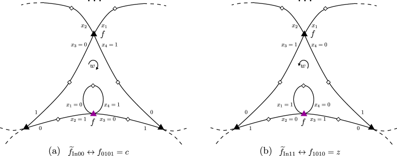
Figure 4.3: A self-loop on the cycle representing variable $w$ is created for each constraint ${\widetilde{f}}_{\rm In}(w,w)$. This creates a degree 4 vertex labeled by $f$, with four input variables $(x_{1},x_{2},x_{3},x_{4})$ as described. Note that the self-loop is created locally on the cycle such that it does not affect anything having to do with other cycles. Base on the support of $f$, the values $x_{1}\not=x_{2}$ and $x_{3}\not=x_{4}$. By the $(\neq)$ on the loop, we also have $x_{1}\not=x_{4}$. Hence $(x_{1},x_{2})=(x_{3},x_{4})=(0,1)$ or $(1,0)$. It is clear that the former corrresponds to $w=0$ (clockwise orientation), and the latter corrresponds to $w=1$ (counterclockwise orientation). This is consistent with the association in Figure 4.2.

There is also the possibility that the binary constraint ${\widetilde{f}}_{\rm In}$ is applied to a single variable, say $w$, resulting in a unary constraint that takes value ${\widetilde{f}}_{\rm In}(0,0)=c$ if $w=0$ and ${\widetilde{f}}_{\rm In}(1,1)=z$ if $w=1$. To reflect that, we simply introduce a self-loop on the cycle representing the variable $w$ for every such occurrence, as illustrated in Figure 4.3. It is clear that the values $c$ and $z$ are perfectly mirrored by the values that the local copy $f$ takes under the two orientations for the cycle corresponding to $w=0$ and $1$. ∎

Theorem 4.3.

Let $f$ be a 4-ary signature of the form (4.1). Then $\operatorname{Pl-Holant}(\neq_{2}\mid f)$ is #P-hard unless $f\in\mathscr{P}$, $f\in\mathscr{A}$, or $f\in\mathscr{\widehat{M}}$, in which cases the problem is tractable.

Proof. Tractability follows from Theorems 2.13 and 2.16. For any $f$ of the form (4.1), note that the support of $f$ is contained in $(x_{1}\neq x_{2})\wedge(x_{3}\neq x_{4})$. We have

$$f(x_{1},x_{2},x_{3},x_{4})=\widetilde{f}_{\rm In}(x_{1},x_{3})\cdot\chi_{x_{1}\neq x_{2}}\cdot\chi_{x_{3}\neq x_{4}},$$

where $\chi$ is the 0-1 indicator function. Thus, ${\widetilde{f}_{\rm In}}\in\mathscr{P}$ or $\mathscr{A}$ is equivalent to ${f}\in\mathscr{P}$ or $\mathscr{A}$. In addition, by Lemmas 2.19 and 2.20, ${\widetilde{f}_{\rm In}}\in\mathscr{\widehat{M}}$ is equivalent to $f\in\mathscr{\widehat{M}}$. Therefore, if $f\notin$ $\mathscr{P},\mathscr{A}$ or $\mathscr{\widehat{M}}$, then ${\widetilde{f}_{\rm In}}$ $\notin$ $\mathscr{P},\mathscr{A}$ or $\mathscr{\widehat{M}}$. By Theorem 2.25, $\operatorname{Pl-\#CSP}({\widetilde{f}_{\rm In}})$ is #P-hard, and then by Lemma 4.2, $\operatorname{Pl-Holant}\left(\neq_{2}\mid f\right)$ is #P-hard. ∎

Remark: One may observe that if $f\in\mathscr{M}$, then $\operatorname{Pl-Holant}\left(\neq_{2}\mid f\right)$ is also tractable as $f$ and $(=_{2})$ are both realized by matchgates. However, Theorem 4.3 already accounted for this case because for signature $f$ of the form (4.1), $f\in\mathscr{M}$ implies $f\in\mathscr{P}$.

Now, we consider the case that the inner pair is a zero pair and no outer pair is a zero pair. Note that a signature in the form (4.2) has support contained in $(x_{1}\neq x_{3})\wedge(x_{2}\neq x_{4})$.

Definition 4.4.

Given a 4-ary signature $f$ with the signature matrix

$$M(f)=\left[\begin{matrix}0&0&0&a\\ 0&b&0&0\\ 0&0&y&0\\ x&0&0&0\\ \end{matrix}\right],$$ (4.2)

where $(a,x)\neq(0,0)$ and $(b,y)\neq(0,0)$, let $\mathcal{G}_{f}$ denote the set of all binary signatures $g_{{}_{f}}$ of the form

$$M(g_{{}_{f}})=\left[\begin{matrix}a^{k_{1}+\ell_{1}}y^{k_{2}+\ell_{2}}x^{k_{3}+\ell_{3}}b^{k_{4}+\ell_{4}}&a^{k_{2}+\ell_{4}}y^{k_{3}+\ell_{1}}x^{k_{4}+\ell_{2}}b^{k_{1}+\ell_{3}}\\ a^{k_{4}+\ell_{2}}y^{k_{1}+\ell_{3}}x^{k_{2}+\ell_{4}}b^{k_{3}+\ell_{1}}&a^{k_{3}+\ell_{3}}y^{k_{4}+\ell_{4}}x^{k_{1}+\ell_{1}}b^{k_{2}+\ell_{2}}\\ \end{matrix}\right],$$

satisfying $k=\ell$, where $k=\sum_{i=1}^{4}k_{i},\ell=\sum_{i=1}^{4}\ell_{i}$ and $k_{1},k_{2},k_{3},k_{4},\ell_{1},\ell_{2},\ell_{3},\ell_{4}\in\mathbb{N}$. Let $\mathcal{H}_{f}$ denote the set of all unary signatures $h_{{}_{f}}$ of the form

$$M(h_{{}_{f}})=\left[\begin{matrix}a^{m_{1}}y^{m_{2}}x^{m_{3}}b^{m_{4}}&a^{m_{3}}y^{m_{4}}x^{m_{1}}b^{m_{2}}\end{matrix}\right],$$

where $m_{1},m_{2},m_{3},m_{4}\in\mathbb{N}$.

Let $k=k_{1}=\ell_{1}=\ell=1$, we get a specific signature $g_{1_{f}}\in\mathcal{G}_{f}$, with $M(g_{1_{f}})=\left[\begin{smallmatrix}a^{2}&by\\ by&x^{2}\\ \end{smallmatrix}\right]$. Let $k=k_{1}=\ell_{3}=\ell=1$, we get another specific signature $g_{2_{f}}\in\mathcal{G}_{f}$, with $M(g_{2_{f}})=\left[\begin{smallmatrix}ax&b^{2}\\ y^{2}&ax\\ \end{smallmatrix}\right]$.

Remark: For any $i,j\in\{1,2,3,4\}$, let $k=k_{i}=\ell_{j}=\ell=1$, we can get $16$ signatures in $\mathcal{G}_{f}$ that have similar signature matrices to $M(g_{1_{f}})$ and $M(g_{2_{f}})$. For example, Choosing $k=k_{3}=\ell_{1}=\ell=1$, we get $g^{\prime}_{2_{f}}(x_{1},x_{2})$ with the signature matrix $M(g^{\prime}_{2_{f}})=\left[\begin{smallmatrix}ax&y^{2}\\ b^{2}&ax\\ \end{smallmatrix}\right]$. Indeed $g^{\prime}_{2_{f}}(x_{1},x_{2})=g_{2_{f}}(x_{2},x_{1})$. In fact, $\mathcal{G}_{f}$ is the closure by the Hadamard product (entry-wise product) of these 16 basic signature matrices.

Lemma 4.5.

Let $f$ be a signature of the form (4.2). Then,

$$\operatorname{Pl-Holant}(\neq_{2}\mid f)\leqslant_{T}\operatorname{\#CSP}(\mathcal{G}_{f}\cup\mathcal{H}_{f}),$$ (4.3)

If $a^{2}=x^{2}\neq 0$, $b^{2}=y^{2}\neq 0$ and $\left(\frac{b}{a}\right)^{8}\neq 1$, then

$$\operatorname{\#CSP}(g_{1_{f}},g_{2_{f}})\leqslant_{T}\operatorname{Pl-Holant}(\neq_{2}\mid f).$$ (4.4)

Proof. We divide the proof into two parts: We show the reduction (4.3) in Part i@, and the reduction (4.4) in Part ii@.

Part i@: Suppose $\Omega=(G,\pi)$ is a given instance of $\operatorname{Pl-Holant}(\neq_{2}\mid f)$, where $G=(U,V,E)$ is a plane bipartite graph. Every vertex $v\in V$ has degree 4, and we list its incident four edges in counterclockwise order. Two edges both incident to a vertex $v\in V$ are called adjacent if they are adjacent in this cyclic order, and non-adjacent otherwise. Two edges in $G$ are called $2$-ary edge twins if they are both incident to a vertex $u\in U$ (of degree $2$), and $4$-ary edge twins if they are non-adjacent but both incident to a vertex $v\in V$ (of degree $4$). Both $2$-ary edge twins and $4$-ary edge twins are called edge twins.

Each edge has a unique $2$-ary edge twin at its endpoint in $U$ of degree $2$ and a unique $4$-ary edge twin at its endpoint in $V$ of degree $4$. The reflexive and transitive closure of the symmetric binary relation edge twin forms a partition of $E$ as an edge disjoint union of circuits: $C_{1},C_{2},\ldots,C_{k}$. Note that $C_{i}$ may include repeated vertices called self-intersection vertices, but no repeated edges. We arbitrarily pick an edge $e_{i}$ of $C_{i}$ to be the leader edge of $C_{i}$. Given the leader edge $e_{i}=(u,v)$ of $C_{i}$, with $u\in U$ and $v\in V$, the direction from $u$ to $v$ defines an orientation of the circuit $C_{i}$. For any edge twins $\{e,e^{\prime}\}$, this orientation defines one edge, say $e^{\prime}$, as the successor of the other if $e^{\prime}$ comes right after $e$ in the orientation. When we list the assignments of edges in a circuit, we list successive values of successors, starting with the leader edge.

For any nonzero term in the sum

$$\operatorname{Pl-Holant}_{\Omega}=\sum_{\sigma:E\rightarrow\{0,1\}}\prod_{w\in U\cup V}f_{w}(\sigma\mid_{E_{(w)}}),$$

the assignment of all edges $\sigma:E\rightarrow\{0,1\}$ can be uniquely extended from its restriction on leader edges $\sigma^{\prime}:\{e_{1},e_{2},\cdots e_{k}\}\rightarrow\{0,1\}$. This is because the support of $f$ is contained in $(x_{1}\neq x_{3})\wedge(x_{2}\neq x_{4})$. Thus, at each vertex $v\in V$, $f_{v}(\sigma\mid_{E_{(v)}})\neq 0$ only if each pair of edge twins in $E_{(v)}$ is assigned value $(0,1)$ or $(1,0)$. The same is true for any vertex $u\in U$ of degree 2, which is labeled $(\neq_{2})$. Thus, if the leader edge $e_{i}$ in $C_{i}$ takes value $0$ or 1 respectively, then all edges on $C_{i}$ must take values $(0,1,0,1,\cdots,0,1)$ or $(1,0,1,0,\cdots,1,0)$ respectively on successive successor edges, starting with $e_{i}$. In particular, all pairs of $4$-ary edge twins in $C_{i}$ take assignment $(0,1)$ when $e_{i}=0$ and $(1,0)$ when $e_{i}=1$ (listing the value of the successor second). Then, we have

$$\operatorname{Pl-Holant}_{\Omega}=\sum_{\sigma^{\prime}:\{e_{1},\cdots,e_{k}\}\rightarrow\{0,1\}}\prod_{v\in V}f_{v}(\widehat{\sigma^{\prime}}\mid_{E_{(v)}}),$$

where $\widehat{\sigma^{\prime}}$ denotes the unique extension of $\sigma^{\prime}$.

For all $1\leq i<j\leq k$, let $V_{i,j}=C_{i}\cap C_{j}$ denote the set of all intersection vertices between $C_{i}$ and $C_{j}$. Denote by $\sigma^{\prime}_{(e_{i},e_{j})}$ an assignment $\{e_{i},e_{j}\}\rightarrow\{0,1\}$. Define a binary function $g_{i,j}$ on $e_{i}$ and $e_{j}$ as follows: For any $b,b^{\prime}\in\{0,1\}$, let

$$g_{i,j}(b,b^{\prime})=\prod_{v\in V_{i,j}}f_{v}(\widehat{\sigma^{\prime}_{(e_{i},e_{j})}}\mid_{E_{(v)}}),$$

where $\widehat{\sigma^{\prime}_{(e_{i},e_{j})}}$ is the unique extension of $\sigma^{\prime}_{(e_{i},e_{j})}$ on the union of edge sets of $C_{i}$ and $C_{j}$ as described above, and $\sigma^{\prime}_{(e_{i},e_{j})}$ is the unique assignment on $\{e_{i},e_{j}\}$ such that $e_{i}\mapsto b$ and $e_{j}\mapsto b^{\prime}$. Since all edges incident to vertices in $V_{i,j}$ are either in $C_{i}$ or $C_{j}$, the assignment values of these edges are determined by $\sigma^{\prime}_{(e_{i},e_{j})}$. Hence, $g_{i,j}$ is well-defined.

We show that $g_{i,j}\in\mathcal{G}_{f}$ by induction on the number $n$ of self-intersection vertices in $C_{i}$. Note that in this proof, $i$ and $j$ (with $i<j$) are not treated symmetrically.

For each vertex $v\in V_{i,j}$, consider the two pairs of edge twins incident to it. We label the edge twins in $C_{i}$ by the variables $(x_{1},x_{3})$ such that $x_{3}$ is the successor of $x_{1}$ in the orientation of $C_{i}$. Hence, for all $v\in V_{i,j}$, these variables $(x_{1},x_{3})$ take the same assignment $(0,1)$ when $e_{i}=0$ and $(1,0)$ when $e_{i}=1$. Then, label the edge twins in $C_{j}$ at $v$ by $(x_{2},x_{4})$ so that the 4 edges at $v$ are ordered $(x_{1},x_{2},x_{3},x_{4})$ in counterclockwise order. This choice of $(x_{2},x_{4})$ is unique given the labeling $(x_{1},x_{3})$.

As we traverse $C_{i}$ according to the orientation of $C_{i}$, locally there is a notion of the left side of $C_{i}$. At any vertex $v\in C_{i}\cap C_{j}$, if we take the traversal of $C_{j}$ according to the orientation of $C_{j}$, it either comes into or goes out of the left side of $C_{i}$. We call $v\in C_{i}\cap C_{j}$ of the former kind “entry-vertices”, and the latter kind “exit-vertices” (see Figure 4.4).

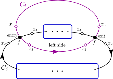
Figure 4.4: Intersection vertices between $C_{i}$ and $C_{j}$

At any entry-vertex $v\in V_{i,j}$, the variable $x_{4}$ is the successor of $x_{2}$, while at any exit-vertex $x_{2}$ is the successor of $x_{4}$. Therefore, at entry-vertices, variables $(x_{2},x_{4})$ take assignment $(0,1)$ when $e_{j}=0$ and $(1,0)$ when $e_{j}=1$, while at exit-vertices they take assignment $(1,0)$ and $(0,1)$ respectively instead.

$(e_{i},e_{j})$	entry-vertices					exit-vertices
	$(x_{1},x_{2},x_{3},x_{4})$	$f$	$f^{\frac{\pi}{2}}$	$f^{\pi}$	$f^{\frac{3\pi}{2}}$	$(x_{1},x_{2},x_{3},x_{4})$	$f$	$f^{\frac{\pi}{2}}$	$f^{\pi}$	$f^{\frac{3\pi}{2}}$
$(0,0)$	$(0,0,1,1)$	$a$	$y$	$x$	$b$	$(0,1,1,0)$	$b$	$a$	$y$	$x$
$(0,1)$	$(0,1,1,0)$	$b$	$a$	$y$	$x$	$(0,0,1,1)$	$a$	$y$	$x$	$b$
$(1,1)$	$(1,1,0,0)$	$x$	$b$	$a$	$y$	$(1,0,0,1)$	$y$	$x$	$b$	$a$
$(1,0)$	$(1,0,0,1)$	$y$	$x$	$b$	$a$	$(1,1,0,0)$	$x$	$b$	$a$	$y$

Table 4.1: The values of $f$ and its rotated copies at intersection vertices

Table 4.1 summarizes the values of $f$ and its rotated copies at intersection vertices $V_{i,j}$. According to the 4 different assignments of $(e_{i},e_{j})$ as listed in column 1 of the table, column 2 and column 7 (indexed by $(x_{1},x_{2},x_{3},x_{4})$) list the assignments of $(x_{1},x_{2},x_{3},x_{4})$ at entry-vertices and exit-vertices separately. With respect to this local labeling of $(x_{1},x_{2},x_{3},x_{4})$, the signature $f$ has four rotated forms:

$$M(f)=\left[\begin{smallmatrix}0&0&0&a\\ 0&b&0&0\\ 0&0&y&0\\ x&0&0&0\\ \end{smallmatrix}\right],M(f^{\frac{\pi}{2}})=\left[\begin{smallmatrix}0&0&0&y\\ 0&a&0&0\\ 0&0&x&0\\ b&0&0&0\\ \end{smallmatrix}\right],M(f^{\pi})=\left[\begin{smallmatrix}0&0&0&x\\ 0&y&0&0\\ 0&0&b&0\\ a&0&0&0\\ \end{smallmatrix}\right]\text{ and }M(f^{\frac{3\pi}{2}})=\left[\begin{smallmatrix}0&0&0&b\\ 0&x&0&0\\ 0&0&a&0\\ y&0&0&0\\ \end{smallmatrix}\right].$$

columns 3, 4, 5, 6 and columns 8, 9, 10, 11 list the corresponding values of the signature $f$ in four forms $f$, $f^{\frac{\pi}{2}}$, $f^{\pi}$ and $f^{\frac{3\pi}{2}}$ respectively.

Suppose there are $k_{1},k_{2},k_{3}$ and $k_{4}$ many entry-vertices assigned $f$, $f^{\frac{\pi}{2}}$, $f^{\pi}$, and $f^{\frac{3\pi}{2}}$, respectively, and there are $\ell_{1},\ell_{2},\ell_{3}$ and $\ell_{4}$ many exit-vertices assigned $f^{\frac{\pi}{2}}$, $f^{\pi}$, $f^{\frac{3\pi}{2}}$ and $f$, respectively. Then, according to the assignments of $(e_{i},e_{j})$, the values of $g_{i,j}$ are listed in Table 4.2, and its signature matrix is given below:

$$M(g_{i,j})=\left[\begin{matrix}a^{k_{1}+\ell_{1}}y^{k_{2}+\ell_{2}}x^{k_{3}+\ell_{3}}b^{k_{4}+\ell_{4}}&a^{k_{2}+\ell_{4}}y^{k_{3}+\ell_{1}}x^{k_{4}+\ell_{2}}b^{k_{1}+\ell_{3}}\\ a^{k_{4}+\ell_{2}}y^{k_{1}+\ell_{3}}x^{k_{2}+\ell_{4}}b^{k_{3}+\ell_{1}}&a^{k_{3}+\ell_{3}}y^{k_{4}+\ell_{4}}x^{k_{1}+\ell_{1}}b^{k_{2}+\ell_{2}}\\ \end{matrix}\right].$$

$(e_{i},e_{j})$	$g_{i,j}(e_{i},e_{j})=f^{k_{1}}(f^{\frac{\pi}{2}})^{k_{2}}(f^{\pi})^{k_{3}}(f^{\frac{3\pi}{2}})^{k_{4}}(f^{\frac{\pi}{2}})^{\ell_{1}}(f^{\pi})^{\ell_{2}}(f^{\frac{3\pi}{2}})^{\ell_{3}}f^{\ell_{4}}$
$(0,0)$	$a^{k_{1}}y^{k_{2}}x^{k_{3}}b^{k_{4}}a^{\ell_{1}}y^{\ell_{2}}x^{\ell_{3}}b^{\ell_{4}}$
$(0,1)$	$b^{k_{1}}a^{k_{2}}y^{k_{3}}x^{k_{4}}y^{\ell_{1}}x^{\ell_{2}}b^{\ell_{3}}a^{\ell_{4}}$
$(1,1)$	$x^{k_{1}}b^{k_{2}}a^{k_{3}}y^{k_{4}}x^{\ell_{1}}b^{\ell_{2}}a^{\ell_{3}}y^{\ell_{4}}$
$(1,0)$	$y^{k_{1}}x^{k_{2}}b^{k_{3}}a^{k_{4}}b^{\ell_{1}}a^{\ell_{2}}y^{\ell_{3}}x^{\ell_{4}}$

Table 4.2: The values of $g_{i,j}$

Our proof that $g_{i,j}\in\mathcal{G}_{f}$ is based on the assertion that the number of “entry-vertices” and “exit-vertices” are equal, namely $\sum_{i=1}^{4}k_{i}=\sum_{i=1}^{4}\ell_{i}$.

• First, consider the base case $n=0$. That is, $C_{i}$ is a simple cycle without self-intersection. By the Jordan Curve Theorem, $C_{i}$ divides the plane into two regions, an interior region and an exterior region. In this case, as we traverse $C_{i}$ according to the orientation of $C_{i}$, the left side of the traversal is always the same region; we call it ${\sf L}_{i}$ (which could be either the interior or the exterior region, depending on the choice of the leader edge $e_{i}$). If we traverse $C_{j}$ according to the orientation of $C_{j}$, we enter and exit the region ${\sf L}_{i}$ an equal number of times. Therefore there is an equal number of “entry-vertices” and “exit-vertices”. Hence $\sum_{i=1}^{4}k_{i}=\sum_{i=1}^{4}\ell_{i}$. It follows that $g_{i,j}\in\mathcal{G}_{f}$ by the definition of $\mathcal{G}_{f}$.

• Inductively, suppose $g_{i,j}\in\mathcal{G}_{f}$ holds for any circuit $C_{i}$ with at most $n$ self-intersections. Let $C_{i}$ have $n+1$ self-intersections. We decompose $C_{i}$ into two edge-disjoint circuits, each of which has at most $n$ self-intersections (See Figure 4.5).

  

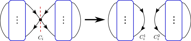
  Figure 4.5: Decompose $C_{i}$ into $C^{1}_{i}$ and $C^{2}_{i}$.

  Take any self-intersection vertex $v^{*}$ of $C_{i}$. There are two pairs of 4-ary edge twins $\{e,e^{\prime}\}$ and $\{\overline{e},\overline{e}^{\prime}\}$, where $e^{\prime}$ is the successor of $e$ and $\overline{e}^{\prime}$ is the successor of $\overline{e}$. Note that $e$ and $\overline{e}$ are oriented toward $v^{*}$, and $e^{\prime}$ and $\overline{e}^{\prime}$ are oriented away from $v^{*}$. By the definition of edge twins, $\{e,\overline{e}\}$ are adjacent, and $\{e^{\prime},\overline{e}^{\prime}\}$ are adjacent. We can break $C_{i}$ into two oriented circuits $C^{1}_{i}$ and $C^{2}_{i}$, by splitting $v^{*}$ into two vertices, and let $e^{\prime}$ follow $\overline{e}$ and let $\overline{e}^{\prime}$ follow $e$. Let the mapping $\gamma:[0,1]\rightarrow\mathbb{R}^{2}$, such that $\gamma(0)=\gamma(1/2)=\gamma(1)=v^{*}$, represent the traversal of $C_{i}$. Then we can define two mappings $\gamma^{1},\gamma^{2}:[0,1]\rightarrow\mathbb{R}^{2}$, such that $\gamma^{1}(t)=\gamma(t/2)$ and $\gamma^{2}(t)=\gamma((t+1)/2)$. Then $\{\gamma^{1},\gamma^{2}\}$ represent $\{C^{1}_{i},C^{2}_{i}\}$ respectively. It follows that $C_{i}$ is the edge disjoint union of $C^{1}_{i}$ and $C^{2}_{i}$ and they both inherit the same orientation from that of $C_{i}$. Any vertex in $V_{i,j}$ is distinct from a self intersection point of $C_{i}$ and thus $V_{i,j}$ is a disjoint union $V^{1}_{i,j}\cup V^{2}_{i,j}$, where $V^{1}_{i,j}=C^{1}_{i}\cap C_{j}$ and $V^{2}_{i,j}=C^{2}_{i}\cap C_{j}$.

  Since $C^{1}_{i}$ inherits the orientation from $C_{i}$, the orientation on $C^{1}_{i}$ is consistent with the orientation starting by choosing a leader edge on $C^{1}_{i}$. The same is true for the orientation on $C^{2}_{i}$. Thus, by induction, on each $C^{1}_{i}\cap C_{j}$ and $C^{2}_{i}\cap C_{j}$ there are an equal number of “entry-vertices” and “exit-vertices”. Hence $\sum_{i=1}^{4}k_{i}=\sum_{i=1}^{4}\ell_{i}$, and so $g_{i,j}\in\mathcal{G}_{f}$, completing the induction.

Let $V_{i}$ be the set of all self-intersections of $C_{i}$. Let $\sigma^{\prime}_{(e_{i})}$ denote the restriction of $\sigma^{\prime}$ on $\{e_{i}\}$. Define a unary function $h_{i}$ on $e_{i}$ as follows: For any $b\in\{0,1\}$, let

$$h_{i}(b)=\prod_{v\in V_{i}}f_{v}(\widehat{\sigma^{\prime}_{(e_{i})}})\mid_{E_{(v)}}),$$

where $\widehat{\sigma^{\prime}_{(e_{i})}}$ is the unique extension of $\sigma^{\prime}_{(e_{i})}$ on the edge set of $C_{i}$, and $\sigma^{\prime}_{(e_{i})}$ is the unique assignment on $\{e_{i}\}$ such that $e_{i}\mapsto b$. The assignment of those edges incident to vertices in $V_{i}$ can be uniquely extended from the assignment $\sigma^{\prime}_{(e_{i})}$. Hence, $h_{i}$ is well-defined. We show that $h_{i}\in\mathcal{H}_{f}$.

For each vertex in $V_{i}$, since it is a self-intersection vertex, the two pairs of edge twins incident to it are both in $C_{i}$. We still first label each pair of edge twins by a pair of variables $(x_{1},x_{3})$ obeying the orientation of $C_{i}$. That is, $x_{3}$ is always the successor of $x_{1}$. Now by the definition of 4-ary edge twins, the two edges labeled $x_{1}$ are adjacent. Hence at each vertex in $V_{i}$, starting from one $x_{1}$, the four incident edges are labeled by $(x_{1},x_{1},x_{3},x_{3})$ in counterclockwise order. We pick the pair of variables $(x_{1},x_{3})$ that appear in the second and fourth positions in this listing and change them to $(x_{2},x_{4})$, so that the four edges are now labeled by $(x_{1},x_{2},x_{3},x_{4})$ in counterclockwise order. Clearly, $(x_{2},x_{4})$ and $(x_{1},x_{3})$ take the same assignment. That is, at each vertex in $V_{i}$, the assignment of $(x_{1},x_{2},x_{3},x_{4})$ is $(0,0,1,1)$ when $e_{i}=0$, and $(1,1,0,0)$ when $e_{i}=1$. Under this labeling, the signature $f$ still has four rotated forms. The values of these four forms are listed in Table 4.3.

$e_{i}$	$(x_{1},x_{2},x_{3},x_{4})$	$f$	$f^{\frac{\pi}{2}}$	$f^{\pi}$	$f^{\frac{3\pi}{2}}$
$0$	$(0,0,1,1)$	$a$	$y$	$x$	$b$
$1$	$(1,1,0,0)$	$x$	$b$	$a$	$y$

Table 4.3: The values of $f$ and its rotated forms at self-intersection vertices

Suppose on $V_{i}$ there are $m_{1},m_{2},m_{3}$ and $m_{4}$ many vertices assigned $f$, $f^{\frac{\pi}{2}}$, $f^{\pi}$ and $f^{\frac{3\pi}{2}}$ respectively. Then, we have

$$M(h_{i})=[\begin{matrix}a^{m_{1}}y^{m_{2}}x^{m_{3}}b^{m_{4}}&a^{m_{3}}y^{m_{4}}x^{m_{1}}b^{m_{2}}\end{matrix}].$$

It follows that $h_{i}\in\mathcal{H}_{f}$.

For any vertex $v\in V$, it is either in some $V_{i,j}$ or some $V_{i}$. Thus,

$$\operatorname{Pl-Holant}_{\Omega} =\sum_{\sigma^{\prime}:\{e_{1},\cdots,e_{k}\}\rightarrow\{0,1\}}\Bigg{(}\prod_{\begin{subarray}{c}v\in V_{i,j}\\ 1\leqslant i<j\leqslant k\end{subarray}}f_{v}(\sigma^{\prime}|E_{(v)})\Bigg{)}\Bigg{(}\prod_{\begin{subarray}{c}v\in V_{i}\\ 1\leqslant i\leqslant k\end{subarray}}f_{v}(\sigma^{\prime}|E_{(v)})\Bigg{)}$$

$$=\sum_{\sigma^{\prime}:\{e_{1},\cdots,e_{k}\}\rightarrow\{0,1\}}\Bigg{(}\prod_{1\leqslant i<j\leqslant k}g_{i,j}(\sigma^{\prime}(e_{i}),\sigma^{\prime}(e_{j}))\Bigg{)}\Bigg{(}\prod_{1\leqslant i\leqslant k}h_{i}(\sigma^{\prime}(e_{i}))\Bigg{)},$$

where $g_{i,j}\in\mathcal{G}_{f}\text{ and }h_{i}\in\mathcal{H}_{f}$. Therefore, Pl-Holant$(\neq_{2}\mid f)\leqslant_{T}$#CSP$(\mathcal{G}_{f}\cup\mathcal{H}_{f}).$

Here, we give some examples for the reduction (4.3).

Example 1. The signature grid $\Omega=(G,\pi)$ for $\operatorname{Pl-Holant}\left(\neq_{2}\mid f\right)$ in Figure 4.6 has two circuits $C_{1}$ (the Square) and $C_{2}$ (the Horizontal Eight) in $G$. We have chosen (arbitrarily) a leader edge $e_{i}$ for each circuit $C_{i}$. In Figure 4.6 they are near the top left corner. Given the leader, the direction from its endpoint of degree $2$ to the endpoint of degree $4$ gives a default orientation of the circuit. Given a nonzero term in the sum Pl-Holant_Ω, as a consequence of the support of $f$, the assignment of edges in each circuit is uniquely determined by the assignment of its leader. That is, any assignment of the leaders $\sigma^{\prime}:\{e_{1},e_{2}\}\rightarrow\{0,1\}$ can be uniquely extended to an assignment of all edges $\sigma:E\rightarrow\{0,1\}$ such that on each circuit the values of $0,1$ alternate.

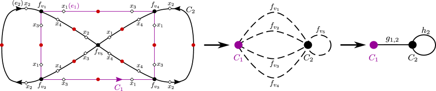
Figure 4.6: A simple example for the reduction (4.3)

Consider the signatures $f_{v_{1}},f_{v_{2}},f_{v_{3}}\text{ and }f_{v_{4}}$ on the intersection vertices between $C_{1}$ and $C_{2}$. Assume $C_{1}$ does not have self-intersection (as is The Square); otherwise, we will decompose $C_{1}$ further and reason inductively. Without self-intersection, $C_{1}$ has an interior and exterior region by the Jordan Curve Theorem. For the chosen orientation of $C_{1}$, its left side happens to be the interior region. With respect to $C_{1}$, the circuit $C_{2}$ enters and exits the interior of $C_{1}$ alternately. Thus, we can divide the intersection vertices into an equal number of “entry-vertices” and “exit-vertices”. In this example, $f_{v_{1}}$ and $f_{v_{4}}$ are on “entry-vertices”, while $f_{v_{2}}$ and $f_{v_{3}}$ are on “exit-vertices”. By analyzing the values of each $f$ when $e_{1}$ and $e_{2}$ take assignment $0$ or $1$, we can view each $f$ as a binary constraint on $(C_{1},C_{2})$. Depending on the $4$ different rotation forms of $f$ and whether $f$ is on “entry-vertices” or “exit-vertices”, the resulting binary constraint has $8$ different forms (See Table 4.1). By multiplying these constraints, we get the binary constraint $g_{1,2}$. This can be viewed as a binary edge function on the circuits $C_{1}$ and $C_{2}$. The property of $g_{1,2}$ crucially depends on there are an equal number of “entry-vertices” and “exit-vertices”. For any $b,b^{\prime}\in\{0,1\}$,

$$g_{1,2}(b,b^{\prime})=\prod_{1\leqslant i\leqslant 4}f_{v_{i}}(\widehat{\sigma^{\prime}_{(e_{1},e_{2})}}\mid_{E_{(v_{i})}}),$$

where $\widehat{\sigma^{\prime}_{(e_{1},e_{2})}}$ uniquely extends to $C_{1}$ and $C_{2}$ the assignment $\sigma^{\prime}_{(e_{1},e_{2})}(e_{1})=b$ and $\sigma^{\prime}_{(e_{1},e_{2})}(e_{2})=b^{\prime}$.

If the placement of $f_{v_{1}}$ were to be rotated clockwise $\frac{\pi}{2}$, then $f_{v_{1}}$ will be changed to $f^{\frac{\pi}{2}}_{v_{1}}$ in the above formula, where $M_{x_{1}x_{2},x_{4}x_{3}}(f^{\frac{\pi}{2}}_{v_{1}})=M_{x_{2}x_{3},x_{1}x_{4}}(f_{v_{1}})$.

For the self-intersection vertex $f_{v_{5}}$, the notions of “entry-vertex” and “exit-vertex” do not apply. $f_{v_{5}}$ gives rise to a unary constraint $h_{2}$ on $e_{2}$. Depending on the $4$ different rotation forms of $f$, $h_{2}$ has $4$ different forms (see Table 3). For any $b\in\{0,1\}$,

$$h_{2}(b)=f_{v_{5}}(\widehat{\sigma^{\prime}_{(e_{2})}}\mid_{E_{(v_{5})}}),$$

where $\widehat{\sigma^{\prime}_{(e_{2})}}$ uniquely extends to $C_{2}$ the assignment $\sigma^{\prime}_{(e_{2})}(e_{2})=b$.

Therefore, we have

$$\operatorname{Pl-Holant}_{\Omega} =\sum_{\sigma:E\rightarrow\{0,1\}}\prod_{v\in V(G)}f_{v}(\sigma\mid_{E_{(v)}})$$

$$=\sum_{\sigma^{\prime}:\{e_{1},e_{2}\}\rightarrow\{0,1\}}\Bigg{(}\prod_{1\leqslant i\leqslant 4}f_{v_{i}}(\sigma^{\prime}|E_{(v_{i})})\Bigg{)}f_{v_{5}}(\sigma^{\prime}|E_{(v_{5})})$$

$$=\sum_{\sigma^{\prime}:\{e_{1},e_{2}\}\rightarrow\{0,1\}}g_{1,2}(\sigma^{\prime}(e_{1}),\sigma^{\prime}(e_{2}))h_{2}(\sigma^{\prime}(e_{2})).$$

Example 2. Figure 4.7 is a more complicated example for the reduction (4.3). The graph in Figure 4.7 (a) is an instance of $\operatorname{Pl-Holant}\left(\neq_{2}\mid f\right)$, where all intersection points are degree 4 vertices labeled by $f$ and we omit the degree 2 vertices labeled by $\neq_{2}$. This graph can be divided into 4 circuits colored by red, blue, purple and green (see Figure 4.7 (b)). Each circuit can be viewed as a Boolean variable for a #CSP problem (see Figure 4.7 (c), edges are constraints).

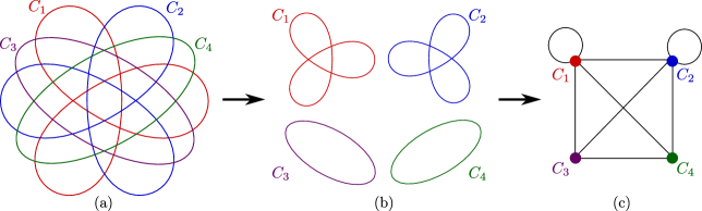
Figure 4.7: A complicated example for the reduction (4.3).

The $0$-$1$ assignment of edges on a circuit $C_{i}$ is uniquely determined by the assignment of its leader edge $e_{i}$, corresponding to two orientations of this circuit. The binary constraint $g_{i,j}$ on $C_{i}$ and $C_{j}$ (for $i<j$) is determined by the placement of signatures $f$ on intersection vertices between circuits $C_{i}$ and $C_{j}$.

Part ii@: Suppose $I$ is a given instance of $\operatorname{\#CSP}(g_{1_{f}},g_{2_{f}})$. Each constraint $g_{1_{f}}$ and $g_{2_{f}}$ is applied on certain pairs of variables. It is possible that they are applied to a single variable, resulting in two unary constraints. We will deal with such constraints later. We first consider the case that every constraint is applied on two distinct variables.

For any pair $i<j$, consider all binary constraints on variables $x_{i}$ and $x_{j}$ $(i<j)$. Note that $g_{1_{f}}$ is symmetric, that is, $g_{1_{f}}(x_{i},x_{j})=g_{1_{f}}(x_{j},x_{i})$. We assume all the constraints between $x_{i}$ and $x_{j}$ are: $s_{i,j}$ many constraints $g_{1_{f}}(x_{i},x_{j})$, $t_{i,j}$ many constraints $g_{2_{f}}(x_{i},x_{j})$ and $t^{\prime}_{i,j}$ many constraints $g_{2_{f}}(x_{j},x_{i})$. Let $g_{i,j}(x_{i},x_{j})$ be the function product of these constraints. That is,

$$g_{i,j}(x_{i},x_{j})=g_{1_{f}}^{s_{i,j}}(x_{i},x_{j})g_{2_{f}}^{t_{i,j}}(x_{i},x_{j})g_{2_{f}}^{t^{\prime}_{i,j}}(x_{j},x_{i}).$$

Then, we have

$$\operatorname{\#CSP}(I)=\sum_{\sigma:\{x_{1},\ldots,x_{k}\}\rightarrow\{0,1\}}\prod_{1\leqslant i<j\leqslant n}g_{i,j}(\sigma(x_{i}),\sigma(x_{j})).$$

We prove the reduction (4.4) in two steps. We first reduce $\operatorname{\#CSP}(I)$ to both instances $\Omega_{i}$ (for $i=1,2$) of $\operatorname{Pl-Holant}\left(\neq_{2}\mid f,\chi_{i}\right)$ respectively, where $\chi_{1}=$ $\left[\begin{smallmatrix}0&0&0&1\\ 0&1&0&0\\ 0&0&1&0\\ 1&0&0&0\\ \end{smallmatrix}\right]$ and $\chi_{2}=$ $\left[\begin{smallmatrix}0&0&0&1\\ 0&1&0&0\\ 0&0&1&0\\ -1&0&0&0\\ \end{smallmatrix}\right]$. The instance $\Omega_{i}$ is constructed as follows:

1. Draw a cycle $D_{1}$, i.e., a homeomorphic image of $S^{1}$, on the plane. For $2\leqslant j\leqslant k$ successively draw cycles $D_{j}$, and for all $1\leqslant i<j$ let $D_{j}$ intersect transversally with $D_{i}$ at least $2(s_{i,j}+t_{i,j}+t^{\prime}_{i,j})$ many times. This can be done since we can let $D_{j}$ enter and exit the interiors of $D_{i}$ successively. A concrete realization is as follows: Place $k$ vertices $D_{i}$ on a semi-circle in the order of $i=1,\ldots,k$. For $1\leqslant i<j\leqslant k$, connect $D_{i}$ and $D_{j}$ by a straight line segment $L_{ij}$. Now thicken each vertex $D_{i}$ into a small disk, and deform the boundary circle of $D_{j}$ so that, for every $1\leqslant i<j$, it reaches across to $D_{i}$ along the line segment $L_{ij}$, and intersects the boundary circle of $D_{i}$ exactly $2(s_{i,j}+t_{i,j}+t^{\prime}_{i,j})$ many times. (There are also other intersections between these cycles $D_{i}$’s due to crossing intersections between those line segments. This is why we say “at least” this many intersections in the overall description. We will deal with those extra intersection vertices later.) We can draw these cycles to satisfy the following conditions:

   1. There is no self-intersection for each $D_{i}$.

   2. Every intersection point is between exactly two cycles. They intersect transversally. Each intersection creates a vertex of degree $4$.

   These intersecting cycles define a planar 4-regular graph $G^{\prime}$, where intersection points are the vertices.

2. Replace each edge of $G^{\prime}$ by a path of length two. We get a planar bipartite graph $G=(V,E)$. On one side, all vertices have degree 2, and on the other side, all vertices have degree 4. We can still define edge twins as in Part i@. Moreover, we still divide the graph into some circuits $C_{1},\ldots,C_{k}$. In fact, $C_{i}$ is just the cycle $D_{i}$ after the replacement of each edge by a path of length two.

   Let $V_{i,j}=C_{i}\cap C_{j}$ $(i<j)$ be the intersection vertices between $C_{i}$ and $C_{j}$. Clearly, $|V_{i,j}|$ is even and at least $2(s_{i,j}+t_{i,j}+t^{\prime}_{i,j})$. Since there is no self-intersection, each circuit is a simple cycle. As we did in Part i@, we pick an edge $e_{i}$ as the leader edge of $C_{i}$ and this gives an orientation of $C_{i}$. We can define “entry-vertices” and “exit-vertices” as in Part i@. Among $V_{i,j}$, half are entry-vertices and the other half are exit-vertices. (This notion is defined in terms of $C_{j}$ with respect to $C_{i}$; the roles of $i$ and $j$ are not symmetric.) List the edges in $C_{i}$ according to the orientation of $C_{i}$ starting with the leader edge $e_{i}$. After we place copies of $f$ on each vertex, the support of $f$, which is contained in $(x_{1}\not=x_{3})\wedge(x_{2}\not=x_{4})$, ensures that every 4-ary twins can only take values $(0,1)$ or $(1,0)$, since the 4-ary twin edges are non-adjacent. Then all edges in $C_{i}$ can only take assignment $(0,1,0,1,\cdots,0,1)$ when $e_{i}=0$ and $(1,0,1,0,\cdots,1,0)$ when $e_{i}=1$.

3. Label all vertices of degree 2 by $(\neq_{2})$. For any vertex in $V_{i,j}$ ($i<j$), as we showed in Part i@, we can label the four edges incident to it by variables $(x_{1},x_{2},x_{3},x_{4})$ in a way such that when $\sigma^{\prime}:(e_{i},e_{j})\mapsto(b,b^{\prime})\in\{0,1\}^{2}$, we have $(x_{1},x_{2},x_{3},x_{4})=(b,b^{\prime},1-b,1-b^{\prime})$ at any entry-vertex, and $(x_{1},x_{2},x_{3},x_{4})=(b,1-b^{\prime},1-b,b^{\prime})$ at any exit-vertex (See Table 4.1). Note that $f$ has four rotation forms under this labeling. We have (at least) $s_{i,j}+t_{i,j}+t^{\prime}_{i,j}$ many entry-vertices and as many exit-vertices. Let $V^{\prime}_{i,j}$ be the set of these $2(s_{i,j}+t_{i,j}+t^{\prime}_{i,j})$ vertices. For vertices in $V^{\prime}_{i,j}$, we label $s_{i,j}$ many entry-vertices by $f$ and $s_{i,j}$ many exit-vertices by $f^{\frac{\pi}{2}}$, $t_{i,j}$ many entry-vertices by $f$ and $t_{i,j}$ many exit-vertices by $f^{\frac{3\pi}{2}}$, and $t^{\prime}_{i,j}$ many entry-vertices by $f^{\pi}$ and $t^{\prime}_{i,j}$ many exit-vertices by $f^{\frac{\pi}{2}}$. Refer to Table 4.2, this choice amounts to taking

   $$k_{1}=s_{i,j}+t_{i,j},\leavevmode\nobreak\ \leavevmode\nobreak\ \leavevmode\nobreak\ \leavevmode\nobreak\ k_{3}=t^{\prime}_{i,j},\leavevmode\nobreak\ \leavevmode\nobreak\ \leavevmode\nobreak\ \leavevmode\nobreak\ \mbox{and,}\leavevmode\nobreak\ \leavevmode\nobreak\ \leavevmode\nobreak\ \leavevmode\nobreak\ \ell_{1}=s_{i,j}+t^{\prime}_{i,j},\leavevmode\nobreak\ \leavevmode\nobreak\ \leavevmode\nobreak\ \leavevmode\nobreak\ \ell_{3}=t_{i,j},$$

   and all other $k_{i}$, $\ell_{i}$’s equal to 0. Recall that $g_{1_{f}}(x_{1},x_{2})$ corresponds to choosing $k_{1}=\ell_{1}=1$ and the others all 0, $g_{2_{f}}(x_{1},x_{2})$ corresponds to choosing $k_{1}=\ell_{3}=1$ and the others all 0, and $g_{2_{f}}(x_{2},x_{1})$ corresponds to choosing $k_{3}=\ell_{1}=1$ and the others all 0, then we have

   $$\prod_{v\in V^{\prime}_{ij}}f_{v}({\sigma^{\prime}_{(e_{i},e_{j})}}\mid_{E_{(v)}})=g_{1_{f}}^{s_{i,j}}(e_{i},e_{j})g_{2_{f}}^{t_{i,j}}(e_{i},e_{j})g_{2_{f}}^{t^{\prime}_{i,j}}(e_{j},e_{i})=g_{i,j}(e_{i},e_{j}).$$

   For all vertices in $V_{i,j}\backslash V^{\prime}_{i,j}$, if we label them by an auxiliary signature $\chi_{1}=\left[\begin{smallmatrix}0&0&0&1\\ 0&1&0&0\\ 0&0&1&0\\ 1&0&0&0\\ \end{smallmatrix}\right],$ then, referring to Table 4.2 (Here $a=x=b=y=1$), we have

   $$\prod_{v\in V_{i,j}\backslash V^{\prime}_{ij}}\chi_{1}(\sigma^{\prime}_{(e_{i},e_{j})}\mid_{E_{(v)}})=1,$$

   for all assignments $\sigma^{\prime}$ on $\{e_{i},e_{j}\}$. We can also label the vertices in $V_{i,j}\backslash V^{\prime}_{i,j}$ by an auxiliary signature $\chi_{2}=\left[\begin{smallmatrix}0&0&0&1\\ 0&1&0&0\\ 0&0&1&0\\ -1&0&0&0\\ \end{smallmatrix}\right].$ By our (semi-circle) construction, in $V_{i,j}\backslash V^{\prime}_{i,j}$, the number of entry-vertices is equal to the number of exit-vertices. We label all entry-vertices by $\chi_{2}$ and label all exit-vertices by its rotated form $\chi^{\frac{\pi}{2}}_{2}=\left[\begin{smallmatrix}0&0&0&1\\ 0&1&0&0\\ 0&0&-1&0\\ 1&0&0&0\\ \end{smallmatrix}\right].$ Refer to Table 4.2 (here $a=b=y=1,x=-1,$ and $k=k_{1}=\ell_{1}=\ell$, and the crucial equation is $g_{i,j}(1,1)=x^{k_{1}+\ell_{1}}=(-1)^{2}=1$), we have

   $$\prod_{v\in V_{i,j}\backslash V^{\prime}_{ij}}\chi_{2}(\sigma^{\prime}_{(e_{i},e_{j})}\mid_{E_{(v)}})=1,$$

   for all assignments $\sigma^{\prime}$ on $\{e_{i},e_{j}\}$.

Then, consider the case that $g_{1_{f}}$ and $g_{2_{f}}$ are applied to the pair variables $(w,w)$, in which case $g_{1_{f}}$ and $g_{2_{f}}$ effectively become unary constraints $[a^{2},x^{2}]$ and $[ax,ax]$ on the variable $x_{i}$. The latter is a constant multiple of $[1,1]$ and can be ignored. The unary constraint $[a,x]$, and hence also $[a^{2},x^{2}]$, can be easily realized by $f$ in $\operatorname{Pl-Holant}(\neq_{2}\mid f,\chi_{i})$, by creating a self-loop for the cycle representing the variable $w$, denoted by $C_{w}$ (See Figure 4.8). Note that the self-loop is created locally on the cycle $C_{w}$ such that it does not affect other cycles. As we did in Part I, we label the four edges incident to a self-intersection vertex by $(x_{1},x_{2},x_{3},x_{4})$ such that $x_{3}$ is the successor of $x_{1}$ and $x_{4}$ is the successor of $x_{2}$ depending on the default orientation of $C_{w}$, and $(x_{1},x_{2},x_{3},x_{4})$ are labeled in counterclockwise order. Then, we have $(x_{1},x_{3})=(x_{2},x_{4})=(0,1)$ when $w=0$ and $(1,0)$ when $w=1$. That is, ${g_{1}}_{f}(0,0)=a^{2}=f^{2}_{0011}$ and ${g_{1}}_{f}(1,1)=x^{2}=f^{2}_{1100}$.

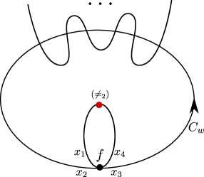
Figure 4.8: Creating self-loop locally on cycle $C_{w}$

Now, we get an instance $\Omega_{s}$ $(s=1,2)$ for each problem $\operatorname{Pl-Holant}\left(\neq_{2}\mid f,\chi_{s}\right)$ respectively. Note that $\chi_{s}$ has the support $(x_{1}\neq x_{3})\wedge(x_{2}\neq x_{4})$ as $f$. As we have showed in Part i@, for any nonzero term in the sum $\operatorname{Pl-Holant}_{\Omega_{s}}$, the assignment of all edges $\sigma:E\rightarrow\{0,1\}$ can be uniquely extended from the assignment of all leader edges $\sigma^{\prime}:\{e_{1},e_{2},\ldots,e_{k}\}\rightarrow\{0,1\}$. Therefore, we have

$$\operatorname{\#CSP}(I) =\sum_{\sigma^{\prime}:\{e_{1},\cdots,e_{k}\}\rightarrow\{0,1\}}\prod_{1\leqslant i<j\leqslant n}g_{i,j}(\sigma^{\prime}(e_{i}),\sigma^{\prime}(e_{j}))$$

$$=\sum_{\sigma^{\prime}:\{e_{1},\cdots,e_{k}\}\rightarrow\{0,1\}}\Bigg{(}\prod_{\begin{subarray}{c}v\in V^{\prime}_{i,j}\\ 1\leqslant i<j\leqslant n\end{subarray}}f_{v}(\sigma^{\prime}|_{E_{(v)}})\Bigg{)}\Bigg{(}\prod_{\begin{subarray}{c}v\in V_{i,j}\backslash V^{\prime}_{i,j}\\ 1\leqslant i<j\leqslant n\end{subarray}}{\chi_{s}}_{v}(\sigma^{\prime}|_{E_{(v)}})\Bigg{)}$$

$$=\operatorname{Pl-Holant}_{\Omega_{s}}$$

for $s=1,2$. That is, $\operatorname{\#CSP}(g_{1_{f}},g_{2_{f}})\leqslant_{T}\operatorname{Pl-Holant}\left(\neq_{2}\mid f,\chi_{s}\right)$, ($s=1,2$).

From the hypothesis of the reduction (4.4), we have $a=\pm x\not=0,b=\pm y\not=0$, and $(b/a)^{8}\not=1$. We show by interpolation

$$\operatorname{Pl-Holant}(\neq_{2}\mid f,\chi_{1})\leqslant_{T}\operatorname{Pl-Holant}(\neq_{2}\mid f)$$

when $a=\epsilon x,b=\epsilon y,$ and

$$\operatorname{Pl-Holant}(\neq_{2}\mid f,\chi_{2})\leqslant_{T}\operatorname{Pl-Holant}(\neq_{2}\mid f)$$

when $a=\epsilon x,b=-\epsilon y$, where $\epsilon=\pm 1$.

• If $a=x$ and $b=y$, since they are all nonzero, and $(\frac{b}{a})^{8}\neq 1$, by normalization we may assume $M(f)=\left[\begin{smallmatrix}0&0&0&1\\ 0&b&0&0\\ 0&0&b&0\\ 1&0&0&0\\ \end{smallmatrix}\right]$, where $b\neq 0$ and $b^{8}\neq 1$.

  If $b$ is not a root of unity, by Lemma 2.3, we have $\operatorname{Pl-Holant}(\neq_{2}\mid f,\chi_{1})\leqslant_{T}\operatorname{Pl-Holant}(\neq_{2}\mid f).$ Otherwise, $b$ is a root of unity. Construct a gadget $f_{\boxtimes}$ as shown in Figure 4.9. Given an assignment $(x_{1},x_{2},x_{3},x_{4})$ to $f_{\boxtimes}$, and suppose $f_{\boxtimes}(x_{1},x_{2},x_{3},x_{4})\neq 0$. Then because of the support of $f_{v_{1}},f_{v_{5}}$ and $f_{v_{3}}$ we must have $x_{1}\neq x_{3}$. Similarly $x_{2}\neq x_{4}$. Also $f_{v_{5}}$ receives the same input as $f_{\boxtimes}$. Hence the support of $f_{\boxtimes}$ is contained in $(x_{1}\neq x_{3})\wedge(x_{2}\neq x_{4})$, i.e., contained in $\{(0,0,1,1),(1,1,0,0),(0,1,1,0),(1,0,0,1)\}$. In particular, the edges on each Diagonal Line of this gadget can only take assignments $(0,1,0,1,0,1)$ or $(1,0,1,0,1,0)$, otherwise the we get zero. On the other hand, the Square cycle in this gadget is a circuit itself, so that the edges in it can only take two assignments $(0,1,0,1,0,1,0,1)$ or $(1,0,1,0,1,0,1,0)$. We simplify the notation to $(0,1)$ and $(1,0)$ respectively. On $(x_{1}\neq x_{3})\wedge(x_{2}\neq x_{4})$, the value of $f_{\boxtimes}$ is the sum over these two terms.

  

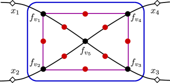
  Figure 4.9: The Square gadget

  For the signature $f$, if one pair of its edge twins flips its assignment between $(0,1)$ and $(1,0)$, then the value of $f$ changes from $1$ to $b$, or from $b$ to $1$. If both pairs of edge twins flip their assignments, then the value of $f$ does not change. According to this property, we give the Table 4.4. Here, we place a suitably rotated copy of $f$ at vertices $v_{i}$ to get $f_{v_{i}}$ (for $1\leq i\leq 5$) so that the values of $f_{v_{i}}$ are all $1$ under the assignment $(x_{1},x_{2},x_{3},x_{4})=(0,0,1,1)$ and the Square is assigned $=(0,1)$ (row 2 of Table 4.4). When the assignment of Square flips from $(0,1)$ to $(1,0)$, one pair of edge twins of each vertex except $v_{5}$ flips its assignment. So the values of $f$ on these vertices except $v_{5}$ change from $1$ to $b$ (row 3). When $(x_{1},x_{3})$ flips its assignment, one pair of edge twins of $v_{1},v_{3}$ and $v_{5}$ flip their assignments. When $(x_{2},x_{4})$ flips its assignment, one pair of edge twins of $v_{2},v_{4}$ and $v_{5}$ flip their assignments. Using this fact, we get other rows correspondingly.

  $(x_{1},x_{2},x_{3},x_{4})$	Square	$f_{v_{1}}$	$f_{v_{2}}$	$f_{v_{3}}$	$f_{v_{4}}$	$f_{v_{5}}$	$f_{\boxtimes}$
  $(0,0,1,1)$	$(0,1)$	$1$	$1$	$1$	$1$	$1$	$1+b^{4}$
  	$(1,0)$	$b$	$b$	$b$	$b$	$1$
  $(1,1,0,0)$	$(0,1)$	$b$	$b$	$b$	$b$	$1$	$1+b^{4}$
  	$(1,0)$	$1$	$1$	$1$	$1$	$1$
  $(0,1,1,0)$	$(0,1)$	$1$	$b$	$1$	$b$	$b$	$2b^{3}$
  	$(1,0)$	$b$	$1$	$b$	$1$	$b$
  $(1,0,0,1)$	$(0,1)$	$b$	$1$	$b$	$1$	$b$	$2b^{3}$
  	$(1,0)$	$1$	$b$	$1$	$b$	$b$

  Table 4.4: The values of gadget $f_{\boxtimes}$ when $a=x=1$ and $b=y$

  Hence, $f_{\boxtimes}$ has the signature matrix $M(f_{\boxtimes})=\left[\begin{smallmatrix}0&0&0&1+b^{4}\\ 0&2b^{3}&0&0\\ 0&0&2b^{3}&0\\ 1+b^{4}&0&0&0\\ \end{smallmatrix}\right]$. Since $b^{8}\neq 1$, we have $1+b^{4}\neq 0$, by normalization we can write $M(f_{\boxtimes})=\left[\begin{smallmatrix}0&0&0&1\\ 0&\frac{2b^{3}}{1+b^{4}}&0&0\\ 0&0&\frac{2b^{3}}{1+b^{4}}&0\\ 1&0&0&0\\ \end{smallmatrix}\right]$. Since $|b|=1$ and $b^{4}\neq 1$, we have $|1+b^{4}|<2$. Then $|\frac{2b^{3}}{1+b^{4}}|>|b^{3}|=1$, which means $\frac{2b^{3}}{1+b^{4}}$ is not a root of unity. By Lemma 2.3, we have $\operatorname{Pl-Holant}(\neq_{2}\mid f,\chi_{1})\leqslant_{T}\operatorname{Pl-Holant}(\neq_{2}\mid f,f_{\boxtimes})$. Since $f_{\boxtimes}$ is constructed by $f$, we have $\operatorname{Pl-Holant}(\neq_{2}\mid f,\chi_{1})\leqslant_{T}\operatorname{Pl-Holant}(\neq_{2}\mid f).$

• If $a=-x$ and $b=-y$, then $M(f)=\left[\begin{smallmatrix}0&0&0&a\\ 0&b&0&0\\ 0&0&-b&0\\ -a&0&0&0\\ \end{smallmatrix}\right]$. Connect the variable $x_{4}$ with $x_{3}$ of $f$ using $(\neq_{2})$, and we get a binary signature $g^{\prime}$, where

  $$g^{\prime}=M_{x_{1}x_{2},x_{4}x_{3}}(0,1,1,0)^{T}=(0,b,-b,0)^{T}.$$

  Since $b\neq 0$, $g^{\prime}$ can be normalized as $(0,1,-1,0)^{T}$. Modifying $x_{1}=1$ of $f$ by $-1$ scaling, we get a signature $f^{\prime}$ with the signature matrix $M(f^{\prime})=\left[\begin{smallmatrix}0&0&0&a\\ 0&b&0&0\\ 0&0&b&0\\ a&0&0&0\\ \end{smallmatrix}\right].$ As we have proved above, $\operatorname{Pl-Holant}(\neq_{2}\mid f,{\chi_{1}})\leqslant_{T}\operatorname{Pl-Holant}(\neq_{2}\mid f,f^{\prime})$. Since $f^{\prime}$ is constructed by $f$, we have $\operatorname{Pl-Holant}(\neq_{2}\mid f,{\chi_{1}})\leqslant_{T}\operatorname{Pl-Holant}(\neq_{2}\mid f).$

• If $a=-x$, $b=y$ or $a=x$, $b=-y$, by normalization and rotational symmetry, we may assume $M(f)=\left[\begin{smallmatrix}0&0&0&1\\ 0&b&0&0\\ 0&0&b&0\\ -1&0&0&0\\ \end{smallmatrix}\right]$, where $b\neq 0$ and $b^{8}\neq 1$.

  If $b$ is not a root of unity, by Corollary 2.4, we have $\operatorname{Pl-Holant}(\neq_{2}\mid f,{\chi_{2}})\leqslant_{T}\operatorname{Pl-Holant}(\neq_{2}\mid f)$. Otherwise, $b$ is a root of unity. Construct the gadget $f_{\boxtimes}$ in the same way as shown above. Our discussion on the support of $f_{\boxtimes}$ still holds: It is contained in $(x_{1}\neq x_{3})\wedge(x_{2}\neq x_{4})$; on $(x_{1},x_{2},x_{3},x_{4})$ with $(x_{1}\neq x_{3})\wedge(x_{2}\neq x_{4})$, $f_{v_{5}}$ receives the same input, and the value of $f_{\boxtimes}$ is the sum over two assignments $(0,1)$ and $(1,0)$ for the Square.

  For the signature $f$, if one pair of its edge twins flips its assignment between $(0,1)$ and $(1,0)$, then the value of $f$ changes from $\pm 1$ to $b$, or $b$ to $\mp 1$. If two pairs of edge twins both flip their assignments, then the value of $f$ does not change if the value is $b$, or changes its sign if the value is $\pm 1$. According to this property, we have the following Table 4.5. Here, we place a suitably rotated copy of $f$ at vertices $v_{i}$ to get $f_{v_{i}}$ (for $1\leq i\leq 5$) so that the values of $f_{v_{i}}$ are all $1$ under the assignment $(x_{1},x_{2},x_{3},x_{4})=(0,0,1,1)$ and the Square is assigned $=(0,1)$ (row 2 of Table 4.5). When the assignment of Square flips from $(0,1)$ to $(1,0)$, one pair of edge twins at each vertex except $v_{5}$ flips its assignment. So the values of $f$ at these vertices except $v_{5}$ change from $1$ to $b$ (row 3). When $(x_{1},x_{3})$ flips its assignment, one pair of edge twins at $v_{1},v_{3}$ and $v_{5}$ flips their assignments. When $(x_{2},x_{4})$ flips its assignment, one pair of edge twins at $v_{2},v_{4}$ and $v_{5}$ flips their assignments. Using this fact, we get other rows correspondingly.

  $(x_{1},x_{2},x_{3},x_{4})$	Square	$f_{v_{1}}$	$f_{v_{2}}$	$f_{v_{3}}$	$f_{v_{4}}$	$f_{v_{5}}$	$f_{\boxtimes}$
  $(0,0,1,1)$	$(0,1)$	$1$	$1$	$1$	$1$	$1$	$1+b^{4}$
  	$(1,0)$	$b$	$b$	$b$	$b$	$1$
  $(1,1,0,0)$	$(0,1)$	$b$	$b$	$b$	$b$	$-1$	$-(1+b^{4})$
  	$(1,0)$	$-1$	$-1$	$-1$	$-1$	$-1$
  $(0,1,1,0)$	$(0,1)$	$1$	$b$	$1$	$b$	$b$	$2b^{3}$
  	$(1,0)$	$b$	$-1$	$b$	$-1$	$b$
  $(1,0,0,1)$	$(0,1)$	$b$	$1$	$b$	$1$	$b$	$2b^{3}$
  	$(1,0)$	$-1$	$b$	$-1$	$b$	$b$

  Table 4.5: The values of gadget $f_{\boxtimes}$ when $a=-x=1$ and $b=y$

  Hence, $f_{\boxtimes}$ has the signature matrix $\left[\begin{smallmatrix}0&0&0&1+b^{4}\\ 0&2b^{3}&0&0\\ 0&0&2b^{3}&0\\ -(1+b^{4})&0&0&0\\ \end{smallmatrix}\right]$. Since $|b|=1$ and $b^{8}\neq 1$, we have $b^{4}\neq\pm 1$, therefore $0<|1+b^{4}|<2$, and so $\frac{2b^{3}}{1+b^{4}}$ is not a root of unity. By Corollary 2.4, $\operatorname{Pl-Holant}(\neq_{2}\mid f,\chi_{2})\leqslant_{T}\operatorname{Pl-Holant}(\neq_{2}\mid f,f_{\boxtimes})$, and hence $\operatorname{Pl-Holant}(\neq_{2}\mid f,\chi_{2})\leqslant_{T}\operatorname{Pl-Holant}(\neq_{2}\mid f).$

In summary, we have

Therefore, we have $\operatorname{\#CSP}(g_{1_{f}},g_{2_{f}})\leqslant_{T}\operatorname{Pl-Holant}\left(\neq_{2}\mid f\right)$ when $a^{2}=x^{2}\neq 0$, $b^{2}=y^{2}\neq 0$ and $(\frac{b}{a})^{8}\neq 1$. ∎

Remark: A crucial point in the reduction (4.3) is the fact that the given instance graph $G$ of $\operatorname{Pl-Holant}\left(\neq_{2}\mid f\right)$ is planar so that $\sum_{i}k_{i}=\sum_{i}\ell_{i}$. Otherwise this does not hold in general; for example the latitudinal and longitudinal closed cycles on a torus intersect at a single point. The equation $\sum_{i}k_{i}=\sum_{i}\ell_{i}$ is crucial to obtain tractability in the following theorem.

Theorem 4.6.

Let $f$ be a 4-ary signature of the form (4.2), where $(a,x)\neq(0,0)$ and $(b,y)\neq(0,0)$. Then $\operatorname{Pl-Holant}(\neq_{2}\mid f)$ is #P-hard unless

1. $(ax)^{2}=(by)^{2}$, or

2. $x=a\mathfrak{i}^{\alpha},b=a\sqrt{\mathfrak{i}}^{\beta},y=a\sqrt{\mathfrak{i}}^{\gamma}$, where $\alpha,\beta,\gamma\in\mathbb{N}$, and $\beta\equiv\gamma\pmod{2},$

in which cases, the problem is tractable in polynomial time.

Proof of Tractability:

• In case (i), if $ax=by=0$, then $f$ has support of size at most $2$. So we have $f\in\mathscr{P}$, and hence $\operatorname{Pl-Holant}(\neq_{2}\mid f)$ is tractable by Theorem 2.13. Otherwise, $(ax)^{2}=(by)^{2}\neq 0$. For any signature $g$ in $\mathcal{G}_{f}$, we have $g_{00}\cdot g_{11}=(ax)^{k_{1}+\ell_{1}+k_{3}+\ell_{3}}(by)^{k_{2}+\ell_{2}+k_{4}+\ell_{4}}$ and $g_{01}\cdot g_{10}=(ax)^{k_{2}+\ell_{2}+k_{4}+\ell_{4}}(by)^{k_{1}+\ell_{1}+k_{3}+\ell_{3}}$. Since $(k_{1}+\ell_{1}+k_{3}+\ell_{3})-(k_{2}+\ell_{2}+k_{4}+\ell_{4})\equiv k+\ell\equiv 0\pmod{2}$, we have

  $$\dfrac{g_{00}\cdot g_{11}}{g_{01}\cdot g_{10}}=\left(\dfrac{ax}{by}\right)^{(k_{1}+\ell_{1}+k_{3}+\ell_{3})-(k_{2}+\ell_{2}+k_{4}+\ell_{4})}=\left(\dfrac{(ax)^{2}}{(by)^{2}}\right)^{\frac{(k_{1}+\ell_{1}+k_{3}+\ell_{3})-(k_{2}+\ell_{2}+k_{4}+\ell_{4})}{2}}=1.$$

  That is, $g\in\mathscr{P}$. Since any signature $h$ in $\mathcal{H}_{f}$ is unary, $h\in\mathscr{P}$. Hence, we have $\mathcal{G}_{f}\cup\mathcal{H}_{f}\subseteq\mathscr{P}$. By Theorem 2.25, #CSP$(\mathcal{G}_{f}\cup\mathcal{H}_{f})$ is tractable. By reduction (4.3) of Lemma 4.5, we have $\operatorname{Pl-Holant}(\neq_{2}\mid f)$ is tractable.

• In case (ii), for any signature $g\in\mathcal{G}_{f}$ defined in Definition 4.4, $M(g)$ is of the form

  $$a^{k+\ell}\left[\begin{matrix}\sqrt{\mathfrak{i}}^{\beta(k_{4}+\ell_{4})+\gamma(k_{2}+\ell_{2})+2\alpha(k_{3}+\ell_{3})}&\sqrt{\mathfrak{i}}^{\beta(k_{1}+\ell_{3})+\gamma(k_{3}+\ell_{1})+2\alpha(k_{4}+\ell_{2})}\\ \sqrt{\mathfrak{i}}^{\beta(k_{3}+\ell_{1})+\gamma(k_{1}+\ell_{3})+2\alpha(k_{2}+\ell_{4})}&\sqrt{\mathfrak{i}}^{\beta(k_{2}+\ell_{2})+\gamma(k_{4}+\ell_{4})+2\alpha(k_{1}+\ell_{1})}\\ \end{matrix}\right]=a^{k+\ell}\left[\begin{matrix}\sqrt{\mathfrak{i}}^{p_{00}}&\sqrt{\mathfrak{i}}^{p_{01}}\\ \sqrt{\mathfrak{i}}^{p_{10}}&\sqrt{\mathfrak{i}}^{p_{11}}\\ \end{matrix}\right],$$

  where $p_{00},p_{01},p_{10}$ and $p_{11}$ denote the integer exponents of $\sqrt{\mathfrak{i}}$ in the respective entries of $g$. Since $\beta\equiv\gamma\pmod{2}$, if they are both even, then $p_{00}\equiv p_{01}\equiv p_{10}\equiv p_{11}\equiv 0\pmod{2};$ if they are both odd, then $p_{00}\equiv p_{11}\equiv k_{2}+\ell_{2}+k_{4}+\ell_{4}\equiv k_{1}+\ell_{1}+k_{3}+\ell_{3}\equiv p_{01}\equiv p_{10}\pmod{2}.$ If these exponents are all odd, we can take out a $\sqrt{\mathfrak{i}}$. Hence, $g$ is of the form $a^{\prime}(\mathfrak{i}^{q_{00}},\mathfrak{i}^{q_{01}},\mathfrak{i}^{q_{10}},\mathfrak{i}^{q_{11}})^{T}$, where $a^{\prime}=a^{k+\ell}$ or $a^{k+\ell}\sqrt{\mathfrak{i}}$, and either $q_{ij}=\frac{p_{ij}}{2}$ for all $i,j\in\{0,1\}$ are integers, or $q_{ij}=\frac{p_{ij}-1}{2}$ for all $i,j\in\{0,1\}$ are integers. Thus,

  $$q_{00}+q_{01}+q_{10}+q_{11}\equiv(p_{00}+p_{01}+p_{10}+p_{11})/2\pmod{2}.$$

  Moreover, since $p_{00}+p_{01}+p_{10}+p_{11}=(k+\ell)(\beta+\gamma+2\alpha)\equiv 0\pmod{4},$ using the assumption that $\beta\equiv\gamma\pmod{2}$ and $k\equiv\ell\pmod{2}$, we conclude that $q_{00}+q_{01}+q_{10}+q_{11}\equiv 0\pmod{2}$. Therefore, $g\in\mathscr{A}$ by Lemma 2.10.

  In this case, for any signature $h$ in $\mathcal{H}_{f}$, $M(h)$ is of the form

  $$a^{m}\left[\begin{matrix}\sqrt{\mathfrak{i}}^{\beta m_{4}+\gamma m_{2}+2\alpha m_{3}}&\sqrt{\mathfrak{i}}^{\beta m_{2}+\gamma m_{4}+2\alpha m_{1}}\end{matrix}\right].$$

  Since $\beta\equiv\gamma\pmod{2}$, we have $\beta m_{4}+\gamma m_{2}\equiv\beta m_{2}+\gamma m_{4}\pmod{2}$. Hence, $h$ is of the form $a^{\prime\prime}[\mathfrak{i}^{q_{0}},\mathfrak{i}^{q_{1}}]$, for some integers $q_{0},q_{1}$, where $a^{\prime\prime}=a^{m}$ or $a^{m}\sqrt{\mathfrak{i}}$. That is, $h\in\mathscr{A}$ by Lemma 2.11. Hence, $\mathcal{G}_{f}\cup\mathcal{H}_{f}\subseteq\mathscr{A}$. By Theorem 2.25, #CSP$(\mathcal{G}_{f}\cup\mathcal{H}_{f})$ is tractable. By reduction (4.3) of Lemma 4.5, we have $\operatorname{Pl-Holant}(\neq_{2}\mid f)$ is tractable.

Proof of Hardness: We are given that $f$ does not belong to case (i) or case (ii). Note that $M_{x_{4}x_{1},x_{3}x_{2}}(f)=\left[\begin{smallmatrix}0&0&0&b\\ 0&x&0&0\\ 0&0&a&0\\ y&0&0&0\\ \end{smallmatrix}\right]$ and $M_{x_{2}x_{3},x_{1}x_{4}}(f)=\left[\begin{smallmatrix}0&0&0&y\\ 0&a&0&0\\ 0&0&x&0\\ b&0&0&0\\ \end{smallmatrix}\right]$. Connect variables $x_{3},x_{2}$ of a copy of the signature $f$ with variables $x_{2},x_{3}$ of another copy of signature $f$ both using $(\neq_{2})$. We get a signature $f_{1}$ with the signature matrix

$$M(f_{1})=M_{x_{4}x_{1},x_{3}x_{2}}(f)NM_{x_{2}x_{3},x_{1}x_{4}}(f)=\left[\begin{matrix}0&0&0&by\\ 0&0&x^{2}&0\\ 0&a^{2}&0&0\\ by&0&0&0\\ \end{matrix}\right].$$

Similarly, connect $x_{3},x_{2}$ of a copy of signature $f$ with $x_{4},x_{1}$ of another copy of signature $f$ both using $(\neq_{2})$. We get a signature $f_{2}$ with the signature matrix

$$M(f_{2})=M_{x_{4}x_{1},x_{3}x_{2}}(f)NM_{x_{4}x_{1},x_{3}x_{2}}(f)=\left[\begin{matrix}0&0&0&b^{2}\\ 0&0&ax&0\\ 0&ax&0&0\\ y^{2}&0&0&0\\ \end{matrix}\right].$$

Notice that $M(f^{\frac{\pi}{2}}_{1})=\left[\begin{smallmatrix}0&0&0&0\\ 0&by&a^{2}&0\\ 0&x^{2}&by&0\\ 0&0&0&0\\ \end{smallmatrix}\right]$, $M(f^{\frac{\pi}{2}}_{2})=\left[\begin{smallmatrix}0&0&0&0\\ 0&b^{2}&ax&0\\ 0&ax&y^{2}&0\\ 0&0&0&0\\ \end{smallmatrix}\right]$, $M(g_{1_{f}})=\left[\begin{smallmatrix}a^{2}&by\\ by&x^{2}\\ \end{smallmatrix}\right]$ and $M(g_{2_{f}})=\left[\begin{smallmatrix}ax&b^{2}\\ y^{2}&ax\\ \end{smallmatrix}\right]$. Recall that $M\left(\widetilde{f^{\frac{\pi}{2}}_{i}}_{\rm{In}}\right)=M_{\rm{In}}(f^{\frac{\pi}{2}}_{i})\left[\begin{smallmatrix}0&1\\ 1&0\\ \end{smallmatrix}\right]$. We have $g_{i_{f}}=\widetilde{{f}^{\frac{\pi}{2}}_{i}}_{\rm{In}}$. That is, $f_{i}(x_{1},x_{2},x_{3},x_{4})=g_{i_{f}}(x_{2},x_{4})\cdot\chi_{x_{1}\neq x_{4}}\cdot\chi_{x_{2}\neq x_{3}}$. Now, we analyze $g_{1_{f}}$ and $g_{2_{f}}$.

• If $\{g_{1_{f}},g_{2_{f}}\}\subseteq\mathscr{P}$, then either $(ax)^{2}=(by)^{2}$ if either signature is degenerate, or $g_{1_{f}}$ and $g_{2_{f}}$ are each generalized Equality or generalized Disequality respectively. In the latter case, since $(a,x)\neq(0,0)$ and $(b,y)\neq(0,0)$, it forces that $ax=by=0$. So we still have $(ax)^{2}=(by)^{2}$. That is, $\{a,b,x,y\}$ belongs to case (i). A contradiction.

• If $\{g_{1_{f}},g_{2_{f}}\}\subseteq\mathscr{A}$, there are two subcases. Note that the support of a function in $\mathscr{A}$ has size a power of 2.

  • If both $g_{1_{f}}$ and $g_{2_{f}}$ have support of size at most $2$, then we have $ax=by=0$ due to $(a,x)\neq(0,0)$ and $(b,y)\neq(0,0)$. This belongs to case (i). A contradiction.

  • Otherwise, at least one of $g_{1_{f}}$ or $g_{2_{f}}$ has support of size $4$. Then $abxy\neq 0$ and therefore both $g_{1_{f}}$ and $g_{2_{f}}$ have support of size $4$. Let $x^{\prime}=\frac{x}{a},b^{\prime}=\frac{b}{a}$ and $y^{\prime}=\frac{y}{a}$. By normalization, we have

    $$M(g_{1_{f}})=a^{2}\left[\begin{matrix}1&b^{\prime}y^{\prime}\\ b^{\prime}y^{\prime}&x^{\prime 2}\\ \end{matrix}\right].$$

    Since $g_{1_{f}}\in\mathscr{A}$, by Lemma 2.10, $x^{\prime 2}$ and $b^{\prime}y^{\prime}$ are both powers of $\mathfrak{i}$, and the sum of all exponents is even. It forces that $x^{\prime 2}=\mathfrak{i}^{2\alpha}$ for some $\alpha\in\mathbb{N}$. Then, we can choose $\alpha$ such $x^{\prime}=\mathfrak{i}^{\alpha}.$ Also, we have

    $$M(g_{2_{f}})=a^{2}\left[\begin{matrix}x^{\prime}&b^{\prime 2}\\ y^{\prime 2}&x^{\prime}\\ \end{matrix}\right].$$

    Since $g_{2_{f}}\in\mathscr{A}$ and $x^{\prime}$ is already a power of $\mathfrak{i}$, $y^{\prime 2}$ and $b^{\prime 2}$ are both powers of $\mathfrak{i}$. That is, $b^{\prime}=\sqrt{\mathfrak{i}}^{\beta}$ and $y^{\prime}=\sqrt{\mathfrak{i}}^{\gamma}$. Also, since $g_{1_{f}}\in\mathscr{A}$, $b^{\prime}y^{\prime}=\sqrt{\mathfrak{i}}^{\beta+\gamma}$ is a power of $\mathfrak{i}$, which means $\beta\equiv\gamma\pmod{2}.$ That is, $\{a,b,x,y\}$ belongs to case (ii). A contradiction.

• If $\{g_{1_{f}},g_{2_{f}}\}\subseteq\mathscr{\widehat{M}}$, then by Lemma 2.19, we have both $a^{2}=\epsilon x^{2},by=\epsilon by$ and $ax=\epsilon^{\prime}ax,y^{2}=\epsilon^{\prime}b^{2}$, for some $\epsilon,\epsilon^{\prime}\in\{1,-1\}$. If $\epsilon=-1$ then $by=0$, and then by the second set of equations $b=y=0$, contrary to assumption that $(b,y)\neq(0,0)$. So $\epsilon=1$. Similarly $\epsilon^{\prime}=1$. Hence

  $$a^{2}=x^{2}\leavevmode\nobreak\ \leavevmode\nobreak\ \leavevmode\nobreak\ \leavevmode\nobreak\ b^{2}=y^{2},$$ (4.5)

  and it also follows that all 4 entries are nonzero.

Therefore, if $\{a,b,x,y\}$ does not satisfy (4.5) then $\{g_{1_{f}},g_{2_{f}}\}\nsubseteq\mathscr{P},\mathscr{A}$ or $\mathscr{\widehat{M}}$. By Theorem 2.25, Pl-#CSP$(g_{1_{f}},g_{2_{f}})$ is #P-hard. Then by Lemma 4.2, $\operatorname{Pl-Holant}(\neq_{2}\mid f^{\frac{\pi}{2}}_{1},f^{\frac{\pi}{2}}_{2})$ is #P-hard, and hence $\operatorname{Pl-Holant}(\neq_{2}\mid f)$ is #P-hard.

Otherwise, the 4 nonzero entries $\{a,b,x,y\}$ satisfy (4.5). If $(\frac{b}{a})^{8}=1$, i.e., $b=a\sqrt{\mathfrak{i}}^{\beta}$ for some $\gamma\in\mathbb{N}$, then $x=\pm a=a{\mathfrak{i}}^{\alpha}$, and $y=\pm b=a\sqrt{\mathfrak{i}}^{\beta+4\delta}$ for some $\alpha,\delta\in\mathbb{N}$. It follows that $\{a,b,x,y\}$ satisfies (ii), a contradiction.

So $(\frac{b}{a})^{8}\neq 1$, and we can apply reduction (4.4) of Lemma 4.5. By the reduction (4.4), we have $\operatorname{\#CSP}(g_{1_{f}},g_{2_{f}})\leqslant_{T}\operatorname{Pl-Holant}(\neq_{2}\mid f).$ Moreover, since $\{a,b,x,y\}$ does not belong to case (i) or case (ii), we have $\{g_{1_{f}},g_{2_{f}}\}\nsubseteq\mathscr{P}$ or $\mathscr{A}$. By Theorem 2.25, $\operatorname{\#CSP}(g_{1_{f}},g_{2_{f}})$ is #P-hard. Therefore, we have $\operatorname{Pl-Holant}(\neq_{2}\mid f)$ is #P-hard. ∎

Corollary 4.7.

Let $f$ be a 4-ary signature of the form (4.2), where $(a,x)\neq(0,0)$ and $(b,y)\neq(0,0)$. If $|ax|\not=|by|$ then $\operatorname{Pl-Holant}(\neq_{2}\mid f)$ is #P-hard.

5 Case iii@: ${\sf N}=2$ with No Zero Pair or ${\sf N}=1$ with Zero in an Outer Pair

If there are exactly two zeros ${\sf N}=2$ with no zero pair, then the two zeros are in different pairs, at least one of them must be in an outer pair. So in Case iii@ there is a zero in an outer pair regardless ${\sf N}=1$ or ${\sf N}=2$. By rotational symmetry, we may assume $a=0$, and we prove this case in Theorem 5.2. We first give the following lemma.

Lemma 5.1.

Let $f$ be a 4-ary signature with the signature matrix $M(f)=\left[\begin{smallmatrix}0&0&0&0\\ 0&b&c&0\\ 0&z&y&0\\ 0&0&0&0\\ \end{smallmatrix}\right]$, where $\det M_{\rm{In}}(f)=by-cz\neq 0$. Let $g$ be a 4-ary signature with the signature matrix $M(g)=\left[\begin{smallmatrix}0&0&0&0\\ 0&0&1&0\\ 0&1&0&0\\ 0&0&0&0\\ \end{smallmatrix}\right].$ Then for any signature set $\mathcal{F}$ containing $f$, we have

$$\operatorname{Pl-Holant}(\neq_{2}\mid\mathcal{F}\cup\{g\})\leqslant_{T}\operatorname{Pl-Holant}(\neq_{2}\mid\mathcal{F}).$$

Proof. We construct a series of gadgets $f_{s}$ by a chain of $s$ copies of $f$ linked by double Disequality $N$. $f_{s}$ has the signature matrix

$$M(f_{s})=M(f)(NM(f))^{s-1}=N(NM(f))^{s}=N\left[\begin{array}[]{cccc}0&\bf{0}&0\\ \mathbf{0}&{\left[\begin{array}[]{cc}z&y\\ b&c\end{array}\right]^{s}}&\mathbf{0}\\ 0&\bf{0}&0\end{array}\right].$$

The inner matrix of $NM(f)$ is $N_{\text{In}}M_{\text{In}}(f)=\left[\begin{smallmatrix}z&y\\ b&c\end{smallmatrix}\right]$. Suppose its spectral decomposition is $Q^{-1}\Lambda Q$, where $\Lambda=[\begin{smallmatrix}\lambda_{1}&\mu\\ 0&\lambda_{2}\\ \end{smallmatrix}]$ is the Jordan Canonical Form. Note that $\lambda_{1}\lambda_{2}=\det\Lambda=\det(N_{\text{In}}M_{\text{In}}(f))\neq 0$. We have $M(f_{s})=NP^{-1}\Lambda_{s}P$, where

$$P=\left[\begin{array}[]{ccc}1&\bf{0}&0\\ \mathbf{0}&Q&\mathbf{0}\\ 0&\bf{0}&1\end{array}\right]\leavevmode\nobreak\ \leavevmode\nobreak\ \leavevmode\nobreak\ \leavevmode\nobreak\ \mbox{and}\leavevmode\nobreak\ \leavevmode\nobreak\ \leavevmode\nobreak\ \leavevmode\nobreak\ \Lambda_{s}=\left[\begin{array}[]{cccc}0&\bf{0}&0\\ \mathbf{0}&{\left[\begin{array}[]{cc}\lambda_{1}&\mu\\ 0&\lambda_{2}\end{array}\right]^{s}}&\mathbf{0}\\ 0&\bf{0}&0\end{array}\right].$$

1. Suppose $\mu=0$, and $\frac{\lambda_{2}}{\lambda_{1}}$ is a root of unity, with $(\frac{\lambda_{2}}{\lambda_{1}})^{n}=1$. Then $\Lambda_{n}=\left[\begin{smallmatrix}0&0&0&0\\ 0&\lambda_{1}^{n}&0&0\\ 0&0&\lambda_{2}^{n}&0\\ 0&0&0&0\end{smallmatrix}\right]=\left[\begin{smallmatrix}0&0&0&0\\ 0&\lambda_{1}^{n}&0&0\\ 0&0&\lambda_{1}^{n}&0\\ 0&0&0&0\end{smallmatrix}\right]$, and $M(f_{n})=\left[\begin{smallmatrix}0&0&0&0\\ 0&0&\lambda_{1}^{n}&0\\ 0&\lambda_{1}^{n}&0&0\\ 0&0&0&0\end{smallmatrix}\right]=\lambda_{1}^{n}\left[\begin{smallmatrix}0&0&0&0\\ 0&0&1&0\\ 0&1&0&0\\ 0&0&0&0\end{smallmatrix}\right].$ After normalization, we can realize the signature $g$.

2. Suppose $\mu=0$, and $\frac{\lambda_{2}}{\lambda_{1}}$ is not a root of unity. The matrix $\Lambda_{s}=\left[\begin{smallmatrix}0&0&0&0\\ 0&\lambda_{1}^{s}&0&0\\ 0&0&\lambda_{2}^{s}&0\\ 0&0&0&0\end{smallmatrix}\right]$ has a good form for interpolation. Suppose $g$ appears $m$ times in an instance $\Omega$ of $\operatorname{Pl-Holant}(\neq_{2}\mid\mathcal{F}\cup\{g\})$. Replace each appearance of $g$ by a copy of the gadget $f_{s}$ to get an instance $\Omega_{s}$ of $\operatorname{Pl-Holant}(\neq_{2}\mid\mathcal{F}\cup\{f_{s}\})$, which is also an instance of $\operatorname{Pl-Holant}(\neq_{2}\mid\mathcal{F})$. We can treat each of the $m$ appearances of $f_{s}$ as a new gadget composed of four functions in sequence $N$, $P^{-1}$, $\Lambda_{s}$ and $P$, and denote this new instance by $\Omega^{\prime}_{s}$. We divide $\Omega^{\prime}_{s}$ into two parts. One part consists of $m$ signatures $\Lambda_{s}^{\otimes{m}}$. Here $\Lambda_{s}^{\otimes{m}}$ is expressed as a column vector. The other part is the rest of $\Omega^{\prime}_{s}$ and its signature is represented by $A$ which is a tensor expressed as a row vector. Then the Holant value of $\Omega^{\prime}_{s}$ is the dot product $\langle A,\Lambda_{s}^{\otimes{m}}\rangle$, which is a summation over $4m$ bits. That is, the value of the $4m$ edges connecting the two parts. We can stratify all $0,1$ assignments of these $4m$ bits having a nonzero evaluation of a term in Pl-Holant${}_{\Omega^{\prime}_{s}}$ into the following categories:

   • There are $i$ many copies of $\Lambda_{s}$ receiving inputs $0110$;

   • There are $j$ many copies of $\Lambda_{s}$ receiving inputs $1001$;

   where $i+j=m$.

   For any assignment in the category with parameter $(i,j)$, the evaluation of $\Lambda_{s}^{\otimes m}$ is clearly $\lambda^{si}_{1}\lambda^{sj}_{2}=\lambda_{1}^{sm}\left(\frac{\lambda_{2}}{\lambda_{1}}\right)^{sj}$. Let $a_{ij}$ be the summation of values of the part $A$ over all assignments in the category $(i,j)$. Note that $a_{ij}$ is independent from the value of $s$ since we view the gadget $\Lambda_{s}$ as a block. Since $i+j=m$, we can denote $a_{ij}$ by $a_{j}$. Then we rewrite the dot product summation and get

   $$\operatorname{Pl-Holant}_{\Omega_{s}}=\operatorname{Pl-Holant}_{\Omega^{\prime}_{s}}=\langle A,\Lambda_{s}^{\otimes{m}}\rangle=\lambda_{1}^{sm}\sum_{0\leqslant j\leqslant m}a_{j}\left(\frac{\lambda_{2}}{\lambda_{1}}\right)^{sj}.$$

   Note that $M(g)=NP^{-1}(NM(g))P$, where $NM(g)=\left[\begin{smallmatrix}0&0&0&0\\ 0&1&0&0\\ 0&0&1&0\\ 0&0&0&0\end{smallmatrix}\right]$. Similarly, divide $\Omega$ into two parts. Under this stratification, we have

   $$\operatorname{Pl-Holant}_{\Omega}=\langle A,(NM(g))^{\otimes{m}}\rangle=\sum_{0\leqslant j\leqslant m}a_{j}.$$

   Since $\frac{\lambda_{2}}{\lambda_{1}}$ is not a root of unity, the Vandermonde coefficient matrix

   $$\left[\begin{matrix}\rho^{0}&\rho^{1}&\cdots&\rho^{m}\\ \rho^{0}&\rho^{2}&\cdots&\rho^{2m}\\ \vdots&\vdots&\vdots&\vdots\\ \rho^{0}&\rho^{m+1}&\cdots&\rho^{(m+1)m}\end{matrix}\right],$$

   has full rank, where $\rho=\frac{\lambda_{2}}{\lambda_{1}}$. Hence, by oracle querying the values of $\operatorname{Pl-Holant}_{\Omega_{s}}$, we can solve for $a_{j}$, and thus obtain the value of $\operatorname{Pl-Holant}_{\Omega}$ in polynomial time.

3. Suppose $\mu=1$, and $\lambda_{1}=\lambda_{2}$ denoted by $\lambda$. Then $\Lambda_{s}=\left[\begin{smallmatrix}0&0&0&0\\ 0&\lambda^{s}&s\lambda^{s-1}&0\\ 0&0&\lambda^{s}&0\\ 0&0&0&0\end{smallmatrix}\right].$ We use this form to give a polynomial interpolation. As in the case above, we can stratify the assignments of $\Lambda_{s}^{\otimes{m}}$ of these $4m$ bits having a nonzero evaluation of a term in Pl-Holant${}_{\Omega^{\prime}_{s}}$ into the following categories:

   • There are $i$ many copies of $\Lambda_{s}$ receiving inputs $0110$ or $1001$;

   • There are $j$ many copies of $\Lambda_{s}$ receiving inputs $0101$;

   where $i+j=m$.

   For any assignment in the category with parameter $(i,j)$, the evaluation of $\Lambda_{s}^{\otimes m}$ is clearly $\lambda^{si}(s\lambda^{s-1})^{j}=\lambda^{sm}(\frac{s}{\lambda})^{j}$. Let $a_{ij}$ be the summation of values of the part $A$ over all assignments in the category $(i,j)$. $a_{ij}$ is independent from $s$. Since $i+j=m$, we can denote $a_{ij}$ by $a_{j}$. Then, we rewrite the dot product summation and get

   $$\operatorname{Pl-Holant}_{\Omega_{s}}=\operatorname{Pl-Holant}_{\Omega^{\prime}_{s}}=\langle A,\Lambda_{s}^{\otimes{m}}\rangle=\lambda^{sm}\sum_{0\leqslant j\leqslant m}a_{j}\left(\frac{s}{\lambda}\right)^{j},$$

   for $s\geq 1$. We consider this as a linear system for $1\leq s\leq m+1$. Similarly, divide $\Omega$ into two parts. Under this stratification, we have

   $$\operatorname{Pl-Holant}_{\Omega}=\langle A,(NM(g))^{\otimes{m}}\rangle=a_{0}.$$

   The Vandermonde coefficient matrix

   $$\left[\begin{matrix}\rho_{1}^{0}&\rho_{1}^{1}&\cdots&\rho_{1}^{m}\\ \rho_{2}^{0}&\rho_{2}^{1}&\cdots&\rho_{2}^{m}\\ \vdots&\vdots&\vdots&\vdots\\ \rho_{m+1}^{0}&\rho_{m+1}^{1}&\cdots&\rho_{m}\end{matrix}\right],$$

   has full rank, where $\rho_{s}=s/\lambda$ are all distinct. Hence, we can solve $a_{0}$ in polynomial time and it is the value of $\operatorname{Pl-Holant}_{\Omega}$.

Therefore, we have $\operatorname{Pl-Holant}(\neq_{2}\mid\mathcal{F}\cup\{g\})\leqslant_{T}\operatorname{Pl-Holant}(\neq_{2}\mid\mathcal{F}).$ ∎

Theorem 5.2 gives a classification for Case III.

Theorem 5.2.

Let $f$ be a 4-ary signature with the signature matrix

$M(f)=\left[\begin{matrix}0&0&0&0\\ 0&b&c&0\\ 0&z&y&0\\ x&0&0&0\\ \end{matrix}\right]$,

where $x\neq 0$ and there is at most one number in $\{b,c,y,z\}$ that is $0$. Then $\operatorname{Pl-Holant}(\neq_{2}\mid f)$ is #P-hard unless $f\in\mathscr{M}$, in which case the problem is tractable.

Proof. Tractability follows from Theorem 2.16.

Suppose $f\notin\mathscr{M}$. By Lemma 2.14, $\det M_{\text{{In}}}(f)\neq\det M_{\text{Out}}(f)=0$, that is $\det\left[\begin{smallmatrix}b&c\\ z&y\\ \end{smallmatrix}\right]=by-cz\neq 0$. Note that $M_{x_{1}x_{2},x_{4}x_{3}}(f)=\left[\begin{smallmatrix}0&0&0&0\\ 0&b&c&0\\ 0&z&y&0\\ x&0&0&0\\ \end{smallmatrix}\right]$, $M_{x_{3}x_{4},x_{2}x_{1}}(f)=\left[\begin{smallmatrix}0&0&0&x\\ 0&y&c&0\\ 0&z&b&0\\ 0&0&0&0\\ \end{smallmatrix}\right]$, and $M_{x_{2}x_{3},x_{1}x_{4}}(f)=\left[\begin{smallmatrix}0&0&0&y\\ 0&0&z&0\\ 0&c&x&0\\ b&0&0&0\\ \end{smallmatrix}\right].$ Connect variables $x_{4},x_{3}$ of a copy of signature $f$ with variables $x_{3},x_{4}$ of another copy of signature $f$ both using $(\neq_{2})$. We get a signature $f_{1}$ with the signature matrix

$$M(f_{1})=M_{x_{1}x_{2},x_{4}x_{3}}(f)NM_{x_{3}x_{4},x_{2}x_{1}}(f)=\left[\begin{matrix}0&0&0&0\\ 0&b_{1}&c_{1}&0\\ 0&z_{1}&y_{1}&0\\ 0&0&0&0\\ \end{matrix}\right],$$

where $\left[\begin{smallmatrix}b_{1}&c_{1}\\ z_{1}&y_{1}\\ \end{smallmatrix}\right]=\left[\begin{smallmatrix}b&c\\ z&y\\ \end{smallmatrix}\right]\cdot\left[\begin{smallmatrix}z&b\\ y&c\\ \end{smallmatrix}\right].$ This $f_{1}$ has the form in Lemma 5.1. Here, $\det\left[\begin{smallmatrix}b_{1}&c_{1}\\ z_{1}&y_{1}\\ \end{smallmatrix}\right]=-(by-cz)^{2}\neq 0$. By Lemma 5.1, we have

$$\operatorname{Pl-Holant}(\neq_{2}\mid f,g)\leqslant_{T}\operatorname{Pl-Holant}(\neq_{2}\mid f,f_{1}),$$

where $g$ has the signature matrix $M(g)=\left[\begin{smallmatrix}0&0&0&0\\ 0&0&1&0\\ 0&1&0&0\\ 0&0&0&0\\ \end{smallmatrix}\right].$

• If $bcyz\neq 0$, connect variables $x_{1},x_{4}$ of signature $f$ with variables $x_{1},x_{2}$ of signature $g$ both using $(\neq_{2})$. We get a signature $f_{2}$ with the signature matrix

  $$M(f_{2})=M_{x_{2}x_{3},x_{1}x_{4}}(f)NM_{x_{1}x_{2},x_{4}x_{3}}(g)=\left[\begin{matrix}0&0&0&0\\ 0&0&z&0\\ 0&c&x&0\\ 0&0&0&0\\ \end{matrix}\right].$$

• Otherwise, connect variables $x_{4},x_{3}$ of signature $f$ with variables $x_{1},x_{2}$ of signature $g$ both using $(\neq_{2})$. We get a signature $f_{2}$ with the signature matrix

  $$M(f_{2})=M_{x_{1}x_{2},x_{4}x_{3}}(f)NM_{x_{1}x_{2},x_{4}x_{3}}(g)=\left[\begin{matrix}0&0&0&0\\ 0&b&c&0\\ 0&z&y&0\\ 0&0&0&0\\ \end{matrix}\right],$$

  and there is exactly one entry in $\{b,c,y,z\}$ that is zero.

In both cases, the support of $f_{2}$ has size $3$, which means $f_{2}\notin\mathscr{P},\mathscr{A}$ or $\mathscr{\widehat{M}}$. By Theorem 4.3, $\operatorname{Pl-Holant}(\neq_{2}\mid f_{2})$ is #P-hard. Since

$$\operatorname{Pl-Holant}(\neq_{2}\mid f_{2})\leqslant_{T}\operatorname{Pl-Holant}(\neq_{2}\mid f,g)\leqslant_{T}\operatorname{Pl-Holant}(\neq_{2}\mid f,f_{1})\leqslant_{T}\operatorname{Pl-Holant}(\neq_{2}\mid f),$$

we have $\operatorname{Pl-Holant}(\neq_{2}\mid f)$ is #P-hard. ∎

6 Case iv@: ${\sf N}=1$ with Zero in the Inner Pair or ${\sf N}=0$

By rotational symmetry, if there is one zero in the inner pair, we may assume it is $c=0$, and $abxyz\not=0$. We first consider the case that $x=\epsilon a,y=\epsilon b$ and $z=\epsilon c$, where $\epsilon=\pm 1$.

Lemma 6.1.

Let $f$ be a 4-ary signature with the signature matrix

$$M(f)=\left[\begin{matrix}0&0&0&a\\ 0&b&c&0\\ 0&\epsilon c&\epsilon b&0\\ \epsilon a&0&0&0\\ \end{matrix}\right],\leavevmode\nobreak\ \leavevmode\nobreak\ \leavevmode\nobreak\ \leavevmode\nobreak\ \mbox{ where }\epsilon=\pm 1\mbox{ and }abc\neq 0.$$

Then $\operatorname{Pl-Holant}(\neq_{2}\mid f)$ is #P-hard if $f\notin\mathscr{M}$.

Proof. If $\epsilon=-1$ we first transform the case to $\epsilon=1$ as follows. Connecting the variable $x_{4}$ with $x_{3}$ of $f$ using $(\neq_{2})$ we get a binary signature $g_{1}$, where

$$g_{1}=M_{x_{1}x_{2},x_{4}x_{3}}(f)(0,1,1,0)^{T}=(0,b+c,-(b+c),0)^{T}.$$

Also connecting the variable $x_{1}$ with $x_{2}$ of $f$ using $(\neq_{2})$ we get a binary signature $g_{2}$, where

$$g_{2}=((0,1,1,0)M_{x_{1}x_{2},x_{4}x_{3}}(f))^{T}=(0,b-c,-(b-c),0)^{T}.$$

Since $bc\neq 0$, $b+c$ and $b-c$ cannot be both zero. Without loss of generality, suppose $b+c\neq 0$. By normalization, we have $g_{1}=(0,1,-1,0)^{T}.$ Then, modifying $x_{1}=1$ of $f$ with $-1$ scaling we get a signature with the signature matrix $\left[\begin{smallmatrix}0&0&0&a\\ 0&b&c&0\\ 0&c&b&0\\ a&0&0&0\\ \end{smallmatrix}\right].$ Therefore, it suffices to show #P-hardness for the case $\epsilon=1$.

Since $f\notin\mathscr{M}$, by Lemma 2.14, $c^{2}-b^{2}\neq a^{2}$. We prove #P-hardness in the following three Cases depending on the values of $a,b$ and $c$.

Case 1: Either $c^{2}-b^{2}\neq 0$ and $|c+b|\neq|c-b|$, or $c^{2}-a^{2}\neq 0$ and $|c+a|\neq|c-a|$. By rotational symmetry, we may assume $c^{2}-b^{2}\neq 0$ and $|c+b|\neq|c-b|$. We may normalize $a=1$ and assume $M(f)=\left[\begin{smallmatrix}0&0&0&1\\ 0&b&c&0\\ 0&c&b&0\\ 1&0&0&0\\ \end{smallmatrix}\right]$, where $c^{2}-b^{2}\neq 0$ or $1$.

We construct a series of gadgets $f_{s}$ by a chain of $s$ copies of $f$ linked by double Disequality $N$. $f_{s}$ has the signature matrix

$$M(f_{s})=M(f)(NM(f))^{s-1}=N(NM(f))^{s}=N\left[\begin{array}[]{cccc}1&\bf{0}&0\\ \mathbf{0}&{\left[\begin{array}[]{cc}c&b\\ b&c\end{array}\right]^{s}}&\mathbf{0}\\ 0&\bf{0}&1\end{array}\right].$$

We diagonalize $\left[\begin{smallmatrix}c&b\\ b&c\end{smallmatrix}\right]^{s}$ using $H=\frac{1}{\sqrt{2}}\left[\begin{smallmatrix}1&1\\ 1&-1\end{smallmatrix}\right]$ (note that $H^{-1}=H$), and get $M(f_{s})=NP\Lambda_{s}P$, where

$$P=\left[\begin{array}[]{ccc}1&\bf{0}&0\\ \mathbf{0}&H&\mathbf{0}\\ 0&\bf{0}&1\end{array}\right],\leavevmode\nobreak\ \leavevmode\nobreak\ \leavevmode\nobreak\ \leavevmode\nobreak\ \mbox{and}\leavevmode\nobreak\ \leavevmode\nobreak\ \leavevmode\nobreak\ \leavevmode\nobreak\ \Lambda_{s}=\left[\begin{array}[]{cccc}1&0&0&0\\ 0&(c+b)^{s}&0&0\\ 0&0&(c-b)^{s}&0\\ 0&0&0&1\end{array}\right].$$

The signature matrix $\Lambda_{s}$ has a good form for polynomial interpolation. In the following, we will reduce $\operatorname{Pl-Holant}(\neq_{2}\mid\hat{f})$ to $\operatorname{Pl-Holant}(\neq_{2}\mid f)$, for suitably chosen $M(\hat{f})=\left[\begin{smallmatrix}0&0&0&1\\ 0&\hat{b}&\hat{c}&0\\ 0&\hat{c}&\hat{b}&0\\ 1&0&0&0\\ \end{smallmatrix}\right]$, and use that to prove that $\operatorname{Pl-Holant}(\neq_{2}\mid f)$ is #P-hard.

Suppose $\hat{f}$ appears $m$ times in an instance $\hat{\Omega}$ of $\operatorname{Pl-Holant}(\neq_{2}\mid\hat{f})$. We replace each appearance of $\hat{f}$ by a copy of the gadget $f_{s}$ to get an instance $\Omega_{s}$ of $\operatorname{Pl-Holant}(\neq_{2}\mid f)$. We can treat each of the $m$ appearances of $f_{s}$ as a new gadget composed of four functions in sequence $N$, $P$, $\Lambda_{s}$ and $P$, and denote this new instance by $\Omega^{\prime}_{s}$. We divide $\Omega^{\prime}_{s}$ into two parts. One part consists of $m$ occurrences of $\Lambda_{s}$, which is $\Lambda_{s}^{\otimes{m}}$, and is written as a column vector of dimension $2^{4m}$. The other part is the rest of $\Omega^{\prime}_{s}$ and its signature is expressed by a tensor $A$, written as a row vector of dimension $2^{4m}$. Then the Holant value of $\Omega^{\prime}_{s}$ is the dot product $\langle A,\Lambda_{s}^{\otimes{m}}\rangle$, which is a summation over $4m$ bits, i.e., the values of the $4m$ edges connecting the two parts. We can stratify all $0,1$ assignments of these $4m$ bits having a nonzero evaluation of a term in Pl-Holant${}_{\Omega^{\prime}_{s}}$ into the following categories:

• There are $i$ many copies of $\Lambda_{s}$ receiving inputs $0000$ or $1111$;

• There are $j$ many copies of $\Lambda_{s}$ receiving inputs $0110$;

• There are $k$ many copies of $\Lambda_{s}$ receiving inputs $1001$;

where $i+j+k=m$.

For any assignment in the category with parameter $(i,j,k)$, the evaluation of $\Lambda_{s}^{\otimes m}$ is clearly $(c+b)^{sj}(c-b)^{sk}$. Let $a_{ijk}$ be the summation of values of the part $A$ over all assignments in the category $(i,j,k)$. Note that $a_{ijk}$ is independent of the value of $s$. Since $i+j+k=m$, we can denote $a_{ijk}$ by $a_{jk}$. Then we rewrite the dot product summation and get

$$\operatorname{Pl-Holant}_{\Omega_{s}}=\operatorname{Pl-Holant}_{\Omega^{\prime}_{s}}=\langle A,\Lambda_{s}^{\otimes{m}}\rangle=\sum_{0\leqslant j+k\leqslant m}a_{jk}(c+b)^{sj}(c-b)^{sk}.$$

Under this stratification, correspondingly we can define $\hat{\Omega}^{\prime}$ and $\hat{\Lambda}$ from $\hat{\Omega}$. Then we have

$$\operatorname{Pl-Holant}_{\hat{\Omega}}=\operatorname{Pl-Holant}_{\hat{\Omega}^{\prime}}=\langle A,\hat{\Lambda}^{\otimes{m}}\rangle=\sum_{0\leqslant j+k\leqslant m}a_{jk}(\hat{c}+\hat{b})^{j}(\hat{c}-\hat{b})^{k},$$

where the same set of values $a_{jk}$ appear. Let $\phi=\hat{c}+\hat{b}$ and $\psi=\hat{c}-\hat{b}$. If we can obtain the value of $p(\phi,\psi)=\sum\limits_{0\leqslant j+k\leqslant m}a_{jk}\phi^{j}\psi^{k}$ from oracle queries to $\operatorname{Pl-Holant}_{\Omega_{s}}$ (for $s\geq 1$) in polynomial time, then we will have proved

$$\operatorname{Pl-Holant}(\neq_{2}\mid\hat{f})\leqslant_{T}\operatorname{Pl-Holant}(\neq_{2}\mid f).$$

Let $\alpha=c+b$ and $\beta=c-b$. Since $c^{2}-b^{2}\neq 0$ or $1$, we have $\alpha\neq 0$, $\beta\neq 0$ and $\alpha\beta\neq 1$. Also, by assumption $|c+b|\neq|c-b|$, we have $|\alpha|\neq|\beta|$. Define $L=\{(j,k)\in\mathbb{Z}^{2}\mid\alpha^{j}\beta^{k}=1\}$. This is a sublattice of $\mathbb{Z}^{2}$. Every lattice has a basis. There are 3 cases depending on the rank of $L$.

• $L=\{(0,0)\}$. All $\alpha^{j}\beta^{k}$ are distinct. It is an interpolation reduction in full power. That is, we can interpolate $p(\phi,\psi)$ for any $\phi$ and $\psi$ in polynomial time. Let $\phi=4$ and $\psi=0$, that is $\hat{b}=2$ and $\hat{c}=2$, and hence $M(\hat{f})=\left[\begin{smallmatrix}0&0&0&1\\ 0&2&2&0\\ 0&2&2&0\\ 1&0&0&0\end{smallmatrix}\right].$ That is, $\hat{f}$ is non-singular redundant. By Theorem 2.23, Pl-Holant$(\neq_{2}\mid\hat{f})$ is #P-hard, and hence Pl-Holant$(\neq_{2}\mid f)$ is #P-hard.

• $L$ contains two independent vectors $(j_{1},k_{1})$ and $(j_{2},k_{2})$ over $\mathbb{Q}$. Then the nonzero vectors $j_{2}(j_{1},k_{1})-j_{1}(j_{2},k_{2})=(0,j_{2}k_{1}-j_{1}k_{2})$ and $k_{2}(j_{1},k_{1})-k_{1}(j_{2},k_{2})=(k_{2}j_{1}-k_{1}j_{2},0)$ are in $L$. Hence, both $\alpha$ and $\beta$ are roots of unity. This implies that $|\alpha|=|\beta|=1$, a contradiction.

• $L=\{(ns,nt)\mid n\in\mathbb{Z}\}$, where $s,t\in\mathbb{Z}$ and $(s,t)\neq(0,0)$. Without loss of generality, we may assume $t\geqslant 0$, and $s>0$ when $t=0$. Also, we have $s+t\neq 0$, otherwise $|{\alpha}|=|{\beta}|$, a contradiction. By Lemma 2.7, for any numbers $\phi$ and $\psi$ satisfying $\phi^{s}\psi^{t}=1$, we can obtain $p(\phi,\psi)$ in polynomial time. Since $\phi=\hat{c}+\hat{b}$ and $\psi=\hat{c}-\hat{b}$, we have $\hat{b}=\frac{\phi-\psi}{2}$ and $\hat{c}=\frac{\phi+\psi}{2}$. That is $M(\hat{f})=\left[\begin{smallmatrix}0&0&0&1\\ 0&\frac{\phi-\psi}{2}&\frac{\phi+\psi}{2}&0\\ 0&\frac{\phi+\psi}{2}&\frac{\phi-\psi}{2}&0\\ 1&0&0&0\end{smallmatrix}\right].$ There are three cases depending on the values of $s$ and $t$.

  • $s\geqslant 0$ and $s+t\geqslant 2$. Consider the function $q(x)=(2-x)^{s}x^{t}-1$. Since $s\geqslant 0$ and $t\geqslant 0$, $q(x)$ is a polynomial. Clearly, $1$ is a root and $0$ is not a root. If $q(x)$ has no other roots, then for some constant $\lambda\neq 0$,

    $$q(x)=\lambda(x-1)^{s+t}=(-1)^{s+t}\lambda((2-x)-1)^{s+t}.$$

    (In fact by comparing leading coefficients, $\lambda=(-1)^{s}$.) Notice that $x^{t}|q(x)+1$, while $x^{t}\nmid\lambda(x-1)^{s+t}+1$ for $t\geqslant 2$. Also, notice that $(2-x)^{s}|q(x)+1$, while $(2-x)^{s}\nmid(-1)^{s+t}\lambda((2-x)-1)^{s+t}$ for $s\geqslant 2$. Hence, $t=s=1$, which means $\alpha\beta=1$. Contradiction.

    Therefore, $q(x)$ has a root $x_{0}$, with $x_{0}\neq 1$ or $0$. Let $\psi=x_{0}$ and $\phi=2-x_{0}$. Then $\phi^{s}\psi^{t}=1$ and $M(\hat{f})=\left[\begin{smallmatrix}0&0&0&1\\ 0&1-x_{0}&1&0\\ 0&1&1-x_{0}&0\\ 1&0&0&0\end{smallmatrix}\right].$ Note that $M_{x_{2}x_{3},x_{1}x_{4}}(\hat{f})=\left[\begin{smallmatrix}0&0&0&1-x_{0}\\ 0&1&1&0\\ 0&1&1&0\\ 1-x_{0}&0&0&0\end{smallmatrix}\right]$. Since $1-x_{0}\neq 0$, $\hat{f}$ is non-singular redundant. By Theorem 2.23, $\operatorname{Pl-Holant}(\neq_{2}\mid\hat{f})$ is #P-hard and hence $\operatorname{Pl-Holant}\left(\neq_{2}\mid f\right)$ is #P-hard.

  • $s<0$ and $t>0$. (Note that $s<0$ implies $t>0$.) Consider the function $q(x)=x^{t}-(2-x)^{-s}$. Since $t>0$ and $-s>0$, it is a polynomial. Clearly, $1$ is a root, but neither $0$ nor $2$ is a root. Since $t+s\neq 0$, the highest order term of $q(x)$ is either $x^{t}$ or $-(-x)^{-s}$, which means the coefficient of the highest order term is $\pm 1$. While the constant term of $q(x)$ is $-2^{-s}\neq\pm 1$. Hence, $q(x)$ cannot be of the form $\lambda(x-1)^{\max(t,-s)}$ for some constant $\lambda\neq 0$. Moreover, since $t+s\neq 0$, $\max(t,-s)\geqslant 2$, which means $q(x)$ has a root $x_{0}$, where $x_{0}\neq 0,1,2$. Dividing by the nonzero term $(2-x_{0})^{-s}$ we have $(2-x_{0})^{s}x_{0}^{t}=1$. Now we let $\psi=x_{0}$ and $\phi=2-x_{0}$, and we have $\operatorname{Pl-Holant}\left(\neq_{2}\mid f\right)$ is #P-hard by the same proof as above.

  • $s\geqslant 0$ and $s+t=1$. In this case, we have $(s,t)=(0,1)$ or $(1,0)$ since $t\geqslant 0$.

    • $(s,t)=(1,0)$. Let $\phi=1$ and $\psi=\frac{1}{2}$. Then we have $\phi^{1}\psi^{0}=1$ and $M(\hat{f})=\left[\begin{smallmatrix}0&0&0&1\\ 0&\frac{1}{4}&\frac{3}{4}&0\\ 0&\frac{3}{4}&\frac{1}{4}&0\\ 1&0&0&0\end{smallmatrix}\right]$. Let $M(f^{\prime})=4M_{x_{2}x_{3},x_{1}x_{4}}(\hat{f})=\left[\begin{smallmatrix}0&0&0&1\\ 0&4&3&0\\ 0&3&4&0\\ 1&0&0&0\end{smallmatrix}\right].$ Clearly, $\operatorname{Pl-Holant}(\neq_{2}\mid f^{\prime})\leqslant_{T}\operatorname{Pl-Holant}\left(\neq_{2}\mid f\right)$. For $M(f^{\prime})$, correspondingly we define $\alpha^{\prime}=3+4=7$ and $\beta^{\prime}=3-4=-1$. Obviously, $\alpha^{\prime}\neq 0$, $\beta^{\prime}\neq 0$, $\alpha^{\prime}\beta^{\prime}\neq 1$, and $|\alpha^{\prime}|\neq|\beta^{\prime}|$. Let $L^{\prime}=\{(j,k)\in\mathbb{Z}^{2}\mid\alpha^{\prime j}\beta^{\prime k}=1\}$. Then we have $L^{\prime}=\{(ns^{\prime},nt^{\prime})\mid n\in\mathbb{Z}\}$, where $s^{\prime}=0$ and $t^{\prime}=2$. Therefore, $s^{\prime}\geqslant 0$ and $s^{\prime}+t^{\prime}\geqslant 2$. As we have showed above, we have $\operatorname{Pl-Holant}\left(\neq_{2}\mid f^{\prime}\right)$ is #P-hard, and hence $\operatorname{Pl-Holant}\left(\neq_{2}\mid f\right)$ is #P-hard.

    • $(s,t)=(0,1)$. Let $\phi=3$ and $\psi=1$. Then we have $\phi^{0}\psi^{1}=1$ and $M(\hat{f})=\left[\begin{smallmatrix}0&0&0&1\\ 0&1&2&0\\ 0&2&1&0\\ 1&0&0&0\end{smallmatrix}\right]$. By Theorem 2.24, $\operatorname{Pl-Holant}(\neq_{2}\mid\hat{f})$ is #P-hard, and hence $\operatorname{Pl-Holant}\left(\neq_{2}\mid f\right)$ is #P-hard.

Case 2: If $c^{2}-b^{2}\neq 0$ and $|c+b|=|c-b|$, or $c^{2}-a^{2}\neq 0$ and $|c+a|=|c-a|$. By rotational symmetry, we may assume $c^{2}-b^{2}\neq 0$ and $|c+b|=|c-b|$. Normalizing $f$ by assuming $c=1$, we have $M(f)=\left[\begin{smallmatrix}0&0&0&a\\ 0&b&1&0\\ 0&1&b&0\\ a&0&0&0\\ \end{smallmatrix}\right]$, where $1^{2}-b^{2}\neq 0$ and $1^{2}-b^{2}\neq a^{2}$ due to $f\notin\mathscr{M}$. Since $|1+b|=|1-b|$, $b$ is a pure imaginary number (as $b\not=0$).

Connect variables $x_{4}$, $x_{3}$ of a copy of signature $f$ with variables $x_{1}$, $x_{2}$ of another copy of signature $f$ both using $(\neq_{2})$. We get a signature $f_{1}$ with the signature matrix

$$M(f_{1})=M_{x_{1}x_{2},x_{4}x_{3}}(f)NM_{x_{1}x_{2},x_{4}x_{3}}(f)=\left[\begin{matrix}0&0&0&a^{2}\\ 0&2b&b^{2}+1&0\\ 0&b^{2}+1&2b&0\\ a^{2}&0&0&0\\ \end{matrix}\right].$$

1. If $c^{2}-a^{2}=0$, that is $a^{2}=1$, and then $M(f_{1})=\left[\begin{smallmatrix}0&0&0&1\\ 0&2b&b^{2}+1&0\\ 0&b^{2}+1&2b&0\\ 1&0&0&0\\ \end{smallmatrix}\right].$ Since $b^{2}<0$, we have $(b^{2}+1)^{2}-(2b)^{2}=(b^{2}-1)^{2}>1=(a^{2})^{2}$, which means $f_{1}\notin\mathscr{M}$.

   • If $b^{2}=-1$, then $M(f_{1})=\left[\begin{smallmatrix}0&0&0&1\\ 0&\pm 2\mathfrak{i}&0&0\\ 0&0&\pm 2\mathfrak{i}&0\\ 1&0&0&0\\ \end{smallmatrix}\right]$. By Corollary 4.7, $\operatorname{Pl-Holant}(\neq_{2}\mid f_{1})$ is #P-hard, and hence $\operatorname{Pl-Holant}(\neq_{2}\mid f)$ is #P-hard.

   • If $b^{2}=-2$, then $M(f_{1})=\left[\begin{smallmatrix}0&0&0&1\\ 0&\pm 2\sqrt{2}\mathfrak{i}&-1&0\\ 0&-1&\pm 2\sqrt{2}\mathfrak{i}&0\\ 1&0&0&0\\ \end{smallmatrix}\right].$ Connect two copies of $f_{1}$, and we have a signature $f_{2}$ with the signature matrix

     $$M(f_{2})=M_{x_{1}x_{2},x_{4}x_{3}}(f_{1})NM_{x_{1}x_{2},x_{4}x_{3}}(f_{1})=\left[\begin{matrix}0&0&0&1\\ 0&\mp 4\sqrt{2}\mathfrak{i}&-7&0\\ 0&-7&\mp 4\sqrt{2}\mathfrak{i}&0\\ 1&0&0&0\\ \end{matrix}\right].$$

     It is easy to check that $f_{2}\notin\mathscr{M}$, by Lemma 2.14. Then, $f_{2}$ belongs to Case 1. Therefore, $\operatorname{Pl-Holant}(\neq_{2}\mid f_{2})$ is #P-hard, and hence $\operatorname{Pl-Holant}(\neq_{2}\mid f)$ is #P-hard.

   • If $b^{2}\neq-1$ or $-2$, then $b^{2}+1\neq\pm 1$ due to $b\neq 0$, hence $1^{2}-(b^{2}+1)^{2}\neq 0$. Also, since $b^{2}+1$ is a real number and $b^{2}+1\neq 0$, we have $|(b^{2}+1)+1|\neq|(b^{2}+1)-1|$. Then $f_{1}$, which is not in $\mathscr{M}$ as shown above, has a signature matrix of the form $\left[\begin{smallmatrix}0&0&0&a_{1}\\ 0&b_{1}&c_{1}&0\\ 0&c_{1}&b_{1}&0\\ a_{1}&0&0&0\\ \end{smallmatrix}\right],$ where $a_{1}=a^{2}=1$, $b_{1}=2b$, and $c_{1}=b^{2}+1$, and $a_{1}b_{1}c_{1}\neq 0$, $c_{1}^{2}-a_{1}^{2}\neq 0$ and $|c_{1}+a_{1}|\neq|c_{1}-a_{1}|$. That is, $f_{1}$ belongs to Case 1. Therefore, $\operatorname{Pl-Holant}(\neq_{2}\mid f_{1})$ is #P-hard, and hence $\operatorname{Pl-Holant}(\neq_{2}\mid f)$ is #P-hard.

2. If $c^{2}-a^{2}\neq 0$ and $|c+a|=|c-a|$, i.e., $|1+a|=|1-a|$, then $a\neq 0$ is also a pure imaginary number. Connect variables $x_{1}$, $x_{4}$ of a copy of signature $f$ with variables $x_{2}$, $x_{3}$ of another copy of signature $f$. We get a signature $f_{3}$ with the signature matrix

   $$M(f_{3})=M_{x_{2}x_{3},x_{1}x_{4}}(f)NM_{x_{2}x_{3},x_{1}x_{4}}(f)=\left[\begin{matrix}0&0&0&b^{2}\\ 0&2a&a^{2}+1&0\\ 0&a^{2}+1&2a&0\\ b^{2}&0&0&0\\ \end{matrix}\right].$$

   Note that $f_{3}\in\mathscr{M}$ implies $(a^{2}-1)^{2}=(b^{2})^{2}$. Since $f\notin\mathscr{M}$, $1-a^{2}\neq b^{2}$. Hence, $f_{3}\in\mathscr{M}$ implies $a^{2}-1=b^{2}$. Similarly, $f_{1}\in\mathscr{M}$ implies $b^{2}-1=a^{2}$. Clearly, $f_{1}$ and $f_{3}$ cannot both be in $\mathscr{M}$. Without loss of generality, we may assume $f_{3}\notin\mathscr{M}$.

   • If $a^{2}\neq-1$, then there are two subcases.

     • $(a^{2}+1)^{2}-(b^{2})^{2}=0$. Since $a$ is a pure imaginary number, $|a^{2}+1+2a|=|a+1|^{2}=|a-1|^{2}=|a^{2}+1-2a|$. Then $f_{3}$ has the signature matrix of the form $\left[\begin{smallmatrix}0&0&0&a_{3}\\ 0&b_{3}&c_{3}&0\\ 0&c_{3}&b_{3}&0\\ a_{3}&0&0&0\\ \end{smallmatrix}\right],$ where $a_{3}b_{3}c_{3}\neq 0$, $c_{3}^{2}-b_{3}^{2}=(a^{2}-1)^{2}\neq 0$ since $a$ is pure imaginary, $|c_{3}+b_{3}|=|c_{3}-b_{3}|$ and $c_{3}^{2}-a_{3}^{2}=0$. That is, $f_{3}$ belongs to Case 2.a. Therefore, $\operatorname{Pl-Holant}(\neq_{2}\mid f_{3})$ is #P-hard, and hence $\operatorname{Pl-Holant}(\neq_{2}\mid f)$ is #P-hard.

     • $(a^{2}+1)^{2}-(b^{2})^{2}\neq 0$. Since $a^{2}+1$ and $b^{2}$ are both nonzero real numbers due to $a$ and $b$ are both pure imaginary numbers, we have $|a^{2}+1+b^{2}|\neq|a^{2}+1-b^{2}|$. Then $f_{3}$ has the signature matrix of the form $\left[\begin{smallmatrix}0&0&0&a_{3}\\ 0&b_{3}&c_{3}&0\\ 0&c_{3}&b_{3}&0\\ a_{3}&0&0&0\\ \end{smallmatrix}\right],$ where $a_{3}b_{3}c_{3}\neq 0$, $c_{3}^{2}-a_{3}^{2}\neq 0$ and $|c_{3}+a_{3}|\neq|c_{3}-a_{3}|$. That is, $f_{3}$ belongs to Case 1. Therefore, $\operatorname{Pl-Holant}(\neq_{2}\mid f_{3})$ is #P-hard, and hence $\operatorname{Pl-Holant}(\neq_{2}\mid f)$ is #P-hard.

   • If $a^{2}=-1$ and $b^{2}\neq-2$, then $M(f_{3})=\left[\begin{smallmatrix}0&0&0&b^{2}\\ 0&2a&0&0\\ 0&0&2a&0\\ b^{2}&0&0&0\\ \end{smallmatrix}\right]$, where $|2a|=2\neq|b^{2}|$. By Corollary 4.7, $\operatorname{Pl-Holant}(\neq_{2}\mid f_{3})$ is #P-hard, and hence $\operatorname{Pl-Holant}(\neq_{2}\mid f)$ is #P-hard.

   • If $a^{2}=-1$ and $b^{2}=-2$, then $M(f_{1})=\left[\begin{smallmatrix}0&0&0&-1\\ 0&\pm 2\sqrt{2}\mathfrak{i}&-1&0\\ 0&-1&\pm 2\sqrt{2}\mathfrak{i}&0\\ -1&0&0&0\\ \end{smallmatrix}\right].$ Note that $M_{x_{2}x_{3},x_{1}x_{4}}(f_{1})=\left[\begin{smallmatrix}0&0&0&\pm 2\sqrt{2}\mathfrak{i}\\ 0&-1&-1&0\\ 0&-1&-1&0\\ \pm 2\sqrt{2}\mathfrak{i}&0&0&0\\ \end{smallmatrix}\right],$ which means $f_{1}$ is non-singular redundant. Therefore, we have $\operatorname{Pl-Holant}(\neq_{2}\mid f_{1})$ is #P-hard, and hence $\operatorname{Pl-Holant}(\neq_{2}\mid f)$ is #P-hard.

3. If $c^{2}-a^{2}\neq 0$ and $|c+a|\neq|c-a|$. This is Case 1. Done.

Case 3: $c^{2}-b^{2}=0$ and $c^{2}-a^{2}=0$. If $c=b$ or $c=a$, then $f$ is non-singular redundant, and hence $\operatorname{Pl-Holant}(\neq_{2}\mid f)$ is #P-hard. Otherwise, $a=b=-c$. By normalization, we have $M(f)=\left[\begin{smallmatrix}0&0&0&-1\\ 0&-1&1&0\\ 0&1&-1&0\\ -1&0&0&0\\ \end{smallmatrix}\right]$, and then $M(f_{1})=\left[\begin{smallmatrix}0&0&0&1\\ 0&-2&2&0\\ 0&2&-2&0\\ 1&0&0&0\\ \end{smallmatrix}\right]$. Notice that $2^{2}-1^{2}\neq 0$ and $|2+1|\neq|2-1|$. That is, $f_{1}$ belongs to Case 1. Therefore, $\operatorname{Pl-Holant}(\neq_{2}\mid f_{1})$ is #P-hard, and hence $\operatorname{Pl-Holant}(\neq_{2}\mid f)$ is #P-hard.

Case 1 to Case 3 cover all cases for $(a,b,c)$: Suppose $(a,b,c)$ does not satisfy Case 3. Then either $c^{2}-b^{2}\not=0$ or $c^{2}-a^{2}\not=0$. If $c^{2}-b^{2}\not=0$, then either $|c+b|\not=|c-b|$ (Case 1) or $|c+b|=|c-b|$ (Case 2). Similarly if $c^{2}-a^{2}\not=0$ it is either Case 1 or Case 2. This completes the proof of the lemma. ∎

Lemma 6.2.

Let $f$ be a 4-ary signature with the signature matrix

$M(f)=\left[\begin{matrix}0&0&0&a\\ 0&b&c&0\\ 0&z&y&0\\ x&0&0&0\\ \end{matrix}\right]$,    where   $abcxyz\neq 0$.

If $by-cz=0$ or $ax-cz=0$, then $\operatorname{Pl-Holant}(\neq_{2}\mid f)$ is #P-hard.

Proof. By rotational symmetry, we assume $by-cz=0$. By normalization, we assume $b=1$, and then $y=cz$. That is, $M_{x_{1}x_{2},x_{4}x_{3}}(f)=\left[\begin{smallmatrix}0&0&0&a\\ 0&1&c&0\\ 0&z&cz&0\\ x&0&0&0\\ \end{smallmatrix}\right]$.

• If $1+c\neq 0$. Connecting the variables $x_{4}$ with $x_{3}$ of $f$ using $(\neq_{2})$ we get a binary signature $g_{1}$, where

  $$g_{1}=M_{x_{1}x_{2},x_{4}x_{3}}(f)(0,1,1,0)^{T}=(0,1+c,(1+c)z,0)^{T}.$$

  Note that $g_{1}(x_{1},x_{2})$ can be normalized as $(0,z^{-1},1,0)^{T}$. That is $g(x_{2},x_{1})=(0,1,z^{-1},0)^{T}$. Modifying $x_{1}=1$ of $f$ with $z^{-1}$ scaling we get a signature $f_{1}$ with the signature matrix $\left[\begin{smallmatrix}0&0&0&a\\ 0&1&c&0\\ 0&1&c&0\\ x/z&0&0&0\\ \end{smallmatrix}\right].$ Connecting the variable $x_{1}$ with $x_{2}$ of $f_{1}$ using $(\neq_{2})$ we get a binary signature $g_{2}$, where

  $$g_{2}=((0,1,1,0)M_{x_{1}x_{2},x_{4}x_{3}}(f))^{T}=(0,2,2c,0)^{T},$$

  and $g_{2}(x_{1},x_{2})$ can be normalized to $g_{2}(x_{2},x_{1})=(0,1,c^{-1},0)^{T}$. Modifying $x_{4}=1$ of $f_{1}$ with $c^{-1}$ scaling we get a signature $f_{2}$ with the signature matrix $\left[\begin{smallmatrix}0&0&0&a/c\\ 0&1&1&0\\ 0&1&1&0\\ x/z&0&0&0\\ \end{smallmatrix}\right].$ It is non-singular redundant. By Lemma 2.23, we have $\operatorname{Pl-Holant}(\neq_{2}\mid f_{2})$ is #P-hard, and hence $\operatorname{Pl-Holant}(\neq_{2}\mid f)$ is #P-hard.

• If $1+z\neq 0$, then connecting the variable $x_{1}$ with $x_{2}$ of $f$ using $(\neq_{2})$ we get a binary signature $g^{\prime}_{1}$, where

  $$g^{\prime}_{1}=((0,1,1,0)M_{x_{1}x_{2},x_{4}x_{3}})^{T}=(0,1+z,(1+z)c,0)^{T}.$$

  $g^{\prime}_{1}(x_{1},x_{2})$ can be normalized to $(0,c^{-1},1,0)^{T}$. By the same analysis as in the case $1+c\neq 0$, we have $\operatorname{Pl-Holant}(\neq_{2}\mid f)$ is #P-hard.

• Otherwise, $1+c=0$ and $1+z=0$, that is $c=z=-1$. Then $M_{x_{1}x_{2},x_{4}x_{3}}(f)=\left[\begin{smallmatrix}0&0&0&a\\ 0&1&-1&0\\ 0&-1&1&0\\ x&0&0&0\\ \end{smallmatrix}\right]$, and $M_{x_{3}x_{4},x_{2}x_{1}}(f)=\left[\begin{smallmatrix}0&0&0&x\\ 0&1&-1&0\\ 0&-1&1&0\\ a&0&0&0\\ \end{smallmatrix}\right]$. Connecting variables $x_{4},x_{3}$ of a copy of signature ${f}$ with variables $x_{3},x_{4}$ of another copy of signature $f$, we get a signature ${f_{3}}$ with the signature matrix

  $$M(f_{3})=M_{x_{1}x_{2},x_{4}x_{3}}(f)NM_{x_{3}x_{4},x_{2}x_{1}}(f)=\left[\begin{matrix}0&0&0&ax\\ 0&-2&2&0\\ 0&2&-2&0\\ ax&0&0&0\\ \end{matrix}\right],$$

  Clearly, $ax\neq 0$ and so $f_{3}\notin\mathscr{M}$ by Lemma 2.14. By Lemma 6.1, $\operatorname{Pl-Holant}\left(\neq_{2}\mid f_{3}\right)$ is #P-hard and hence $\operatorname{Pl-Holant}\left(\neq_{2}\mid f\right)$ is #P-hard. ∎

In the following Lemmas 6.3, 6.4, 6.6 and Corollaries 6.5, 6.7, let $f$ be a 4-ary signature with the signature matrix

$$M(f)=\left[\begin{matrix}0&0&0&a\\ 0&b&c&0\\ 0&z&y&0\\ x&0&0&0\\ \end{matrix}\right],$$ (6.6)

where $abxyz\neq 0$, $\det\left[\begin{smallmatrix}b&c\\ z&y\\ \end{smallmatrix}\right]=by-cz\neq 0$ and $\det\left[\begin{smallmatrix}a&z\\ c&x\\ \end{smallmatrix}\right]=ax-cz\neq 0$. Moreover $f\notin\mathscr{M}$, that is $cz-by\neq ax$. These lemmas handle “generic” cases of this section and will culminate in Theorem 6.8, which is a classification for Case iv@. It is here we will use Möbius transformations to handle interpolations where it is particularly difficult to get desired signatures of “infinite order”.

Lemma 6.3.

Let $g=(0,1,t,0)^{T}$ be a binary signature, where $t\neq 0$ is not a root of unity. Then $\operatorname{Pl-Holant}(\neq_{2}\mid f,g)$ is #P-hard.

Proof. Let $\mathcal{B}=\{g_{1},g_{2},g_{3}\}$ be a set of three binary signatures $g_{i}=(0,1,t_{i},0)^{T}$, for some $t_{i}\in\mathbb{C}$. By Lemma 2.5, we have $\operatorname{Pl-Holant}\left(\neq_{2}\mid\{f\}\cup\mathcal{B}\right)\leqslant\operatorname{Pl-Holant}\left(\neq_{2}\mid f,g\right).$ We will show that $\operatorname{Pl-Holant}\left(\neq_{2}\mid\{f\}\cup\mathcal{B}\right)$ is #P-hard and it follows that $\operatorname{Pl-Holant}\left(\neq_{2}\mid f,g\right)$ is #P-hard.

Modifying $x_{1}=1$ of $f$ with $t_{i}$ $(i=1,2)$ scaling separately, we get two signatures $f_{t_{i}}$ with the signature matrices $M(f_{t_{i}})=\left[\begin{smallmatrix}0&0&0&a\\ 0&b&c&0\\ 0&t_{i}z&t_{i}y&0\\ t_{i}x&0&0&0\\ \end{smallmatrix}\right]$. Note that

$$\det M_{\text{In}}(f_{t_{i}})=t_{i}\det M_{\text{In}}(f)\leavevmode\nobreak\ \leavevmode\nobreak\ \leavevmode\nobreak\ \mbox{ and }\leavevmode\nobreak\ \leavevmode\nobreak\ \leavevmode\nobreak\ \det M_{\text{Out}}(f_{t_{i}})=t_{i}\det M_{\text{Out}}(f).$$

Connecting variables $x_{4},x_{3}$ of $f$ with variables $x_{1}$, $x_{2}$ of $f_{t_{1}}$ both using $(\neq_{2})$, we get a signature $f_{1}$ with the signature matrix

$$M(f_{1})=\left[\begin{matrix}0&0&0&a_{1}\\ 0&b_{1}&c_{1}&0\\ 0&z_{1}&y_{1}&0\\ x_{1}&0&0&0\\ \end{matrix}\right]=M(f)NM(f_{t_{1}})=\left[\begin{matrix}0&0&0&a^{2}\\ 0&t_{1}bz+bc&t_{1}by+c^{2}&0\\ 0&t_{1}z^{2}+yb&t_{1}yz+yc&0\\ t_{1}x^{2}&0&0&0\\ \end{matrix}\right].$$

We first show that there is a $t_{1}\neq 0$ such that $b_{1}y_{1}c_{1}z_{1}\neq 0$ and $(b_{1}z)(y_{1}c)-(c_{1}b)(z_{1}y)\neq 0$. Consider the quadratic polynomial

$$p(t)=(tbz+bc)(tyz+yc)cz-(tby+c^{2})(tz^{2}+yb)by.$$

We have $p(t_{1})=(b_{1}z)(y_{1}c)-(c_{1}b)(z_{1}y)$. Notice that the coefficient of the quadratic term in $p(t)$ is $byz^{2}(cz-by)$. It is not equal to zero since $byz^{2}\neq 0$ and $cz-by\neq 0$. That is, $p(t)$ has degree $2$, and hence it has at most two roots. Also we have the following three implications by the definitions of $b_{1},y_{1},c_{1},z_{1}$: $b_{1}y_{1}=0\Longrightarrow t_{1}=-\frac{c}{z}$, $c_{1}=0\Longrightarrow t_{1}=-\frac{c^{2}}{by}$, and $z_{1}=0\Longrightarrow t_{1}=-\frac{yb}{z^{2}}$. Therefore we can choose such a $t_{1}$ that does not take these values $0,-\frac{c}{z},-\frac{c^{2}}{by}$ and $-\frac{yb}{z^{2}}$, and $t_{1}$ is not a root of $p(t)$. Then, we have $t_{1}\neq 0$, $b_{1}y_{1}c_{1}z_{1}\neq 0$ and $(b_{1}z)(y_{1}c)-(c_{1}b)(z_{1}y)\neq 0$.

Connecting variables $x_{4},x_{3}$ of $f_{1}$ with variables $x_{1}$, $x_{2}$ of $f_{t_{2}}$ both using $(\neq_{2})$, we get a signature $f_{2}$ with the signature matrix

$$M(f_{2})=\left[\begin{matrix}0&0&0&a_{2}\\ 0&b_{2}&c_{2}&0\\ 0&z_{2}&y_{2}&0\\ x_{2}&0&0&0\\ \end{matrix}\right]=M(f_{1})NM(f_{t_{2}})=\left[\begin{matrix}0&0&0&a_{1}a\\ 0&t_{2}b_{1}z+c_{1}b&t_{2}b_{1}y+c_{1}c&0\\ 0&t_{2}z_{1}z+y_{1}b&t_{2}z_{1}y+y_{1}c&0\\ t_{2}x_{1}x&0&0&0\\ \end{matrix}\right].$$

Since $b_{1}z\neq 0$ and $c_{1}b\neq 0$, we can let $t_{2}=-\frac{c_{1}b}{b_{1}z}$ and $t_{2}\neq 0$. Then $b_{2}=t_{2}b_{1}z+c_{1}b=0$. Since $(b_{1}z)(y_{1}c)-(c_{1}b)(z_{1}y)\neq 0$, we have $y_{2}=t_{2}z_{1}y+y_{1}c\neq 0$. Notice that

$$\det M_{\text{In}}(f_{2}) =\det M_{\text{In}}(f_{1})\cdot(-1)\cdot\det M_{\text{In}}(f_{t_{2}})$$

$$=\det M_{\text{In}}(f)\cdot(-1)\cdot\det M_{\text{In}}(f_{t_{1}})\cdot(-1)\cdot\det M_{\text{In}}(f_{t_{2}})$$

$$=t_{1}t_{2}\det M_{\text{In}}(f)^{3}$$

$$\neq 0.$$

We have $\det M_{\text{In}}(f_{2})=b_{2}y_{2}-c_{2}z_{2}=-c_{2}z_{2}\neq 0$. Similarly, we have $\det M_{\text{Out}}(f_{2})=-a_{2}x_{2}=t_{1}t_{2}\det M_{\text{Out}}(f)^{3}\neq 0$. Therefore, $M(f_{2})$ is of the form $\left[\begin{smallmatrix}0&0&0&a_{2}\\ 0&0&c_{2}&0\\ 0&z_{2}&y_{2}&0\\ x_{2}&0&0&0\\ \end{smallmatrix}\right]$, where $a_{2}x_{2}y_{2}c_{2}z_{2}\neq 0$. That is, $f_{2}$ is a signature in Case iii@. If $f_{2}\notin\mathscr{M}$, then $\operatorname{Pl-Holant}\left(\neq_{2}\mid f_{2}\right)$ is #P-hard by Theorem 5.2, and hence $\operatorname{Pl-Holant}\left(\neq_{2}\mid\{f\}\cup\mathcal{B}\right)$ is #P-hard.

Otherwise, $f_{2}\in\mathscr{M}$, which means $\dfrac{\det M_{\text{In}}(f_{2})}{\det M_{\text{Out}}(f_{2})}=1.$ Thus $\dfrac{\det M_{\text{In}}(f)^{3}}{\det M_{\text{Out}}(f)^{3}}=1.$ Since $f\notin\mathscr{M}$, $\dfrac{\det M_{\text{In}}(f)}{\det M_{\text{Out}}(f)}\neq 1$, and hence $\dfrac{\det M_{\text{In}}(f)^{7}}{\det M_{\text{Out}}(f)^{7}}\neq 1$. Similar to the construction of $f_{1}$, we construct $f_{3}$. First, modify $x_{1}=1$ of $f_{1}$ with $t_{3}$ scaling. We get a signature $f_{1t_{3}}$ with the signature matrix $M(f_{1t_{3}})=\left[\begin{smallmatrix}0&0&0&a_{1}\\ 0&b_{1}&c_{1}&0\\ 0&t_{3}z_{1}&t_{3}y_{1}&0\\ t_{3}x_{1}&0&0&0\\ \end{smallmatrix}\right]$. Note that $\det M_{\text{In}}(f_{1t_{3}})=t_{3}\det M_{\text{In}}(f_{1})$ and $\det M_{\text{Out}}(f_{1t_{3}})=t_{3}\det M_{\text{Out}}(f_{1})$. Then connect variables $x_{4},x_{3}$ of $f_{1}$ with variables $x_{1}$, $x_{2}$ of $f_{1t_{3}}$ both using $(\neq_{2})$. We get a signature $f_{3}$ with the signature matrix

$$M(f_{3})=\left[\begin{matrix}0&0&0&a_{3}\\ 0&b_{3}&c_{3}&0\\ 0&z_{3}&y_{3}&0\\ x_{3}&0&0&0\\ \end{matrix}\right]=M(f_{1})NM(f_{1t_{3}})=\left[\begin{matrix}0&0&0&a^{2}\\ 0&t_{3}b_{1}z_{1}+b_{1}c_{1}&t_{3}b_{1}y_{1}+c_{1}^{2}&0\\ 0&t_{3}z_{1}^{2}+y_{1}b_{1}&t_{3}y_{1}z_{1}+y_{1}c_{1}&0\\ t_{3}x_{1}^{2}&0&0&0\\ \end{matrix}\right].$$

Since $c_{1}\neq 0$ and $z_{1}\neq 0$, we can define $t_{3}=-\frac{c_{1}}{z_{1}}$ and $t_{3}\neq 0$. Then $b_{3}=b_{1}(t_{3}z_{1}+c_{1})=0$ and $y_{3}=y_{1}(t_{3}z_{1}+c_{1})=0$. Notice that

$$\det M_{\text{In}}(f_{3}) =\det M_{\text{In}}(f_{1})\cdot(-1)\cdot\det M_{\text{In}}(f_{1t_{3}})$$

$$=-\det M_{\text{In}}(f_{1})\cdot t_{3}\det M_{\text{In}}(f_{1})$$

$$=-t_{3}\left[\det M_{\text{In}}(f)\cdot(-1)\cdot\det M_{\text{In}}(f_{t_{1}})\right]^{2}$$

$$=-t_{3}t_{1}^{2}\det M_{\text{In}}(f)^{4}$$

$$\neq 0$$

We have $\det M_{\text{In}}(f_{3})=-c_{3}z_{3}\neq 0$ and similarly, $\det M_{\text{Out}}(f_{3})=-a_{3}x_{3}=-t_{3}t_{1}^{2}\det M_{\text{Out}}(f)^{4}\neq 0$. That is, $M(f_{3})$ is of the form $\left[\begin{smallmatrix}0&0&0&a_{3}\\ 0&0&c_{3}&0\\ 0&z_{3}&0&0\\ x_{3}&0&0&0\\ \end{smallmatrix}\right]$ where $a_{3}x_{3}c_{3}z_{3}\neq 0$.

Connect variables $x_{4},x_{3}$ of $f_{2}$ with variables $x_{1}$, $x_{2}$ of $f_{3}$ both using $(\neq_{2})$. We get a signature $f_{4}$ with the signature matrix

$$M(f_{4})=\left[\begin{matrix}0&0&0&a_{4}\\ 0&b_{4}&c_{4}&0\\ 0&z_{4}&y_{4}&0\\ x_{4}&0&0&0\\ \end{matrix}\right]=M(f_{2})NM(f_{3})=\left[\begin{matrix}0&0&0&a_{2}a_{3}\\ 0&0&c_{2}c_{3}&0\\ 0&z_{2}z_{3}&y_{2}c_{3}&0\\ x_{2}x_{3}&0&0&0\\ \end{matrix}\right].$$

Clearly, $f_{4}$ is a signature in Case iii@. Also, notice that

$$\det M_{\text{In}}(f_{4}) =\det M_{\text{In}}(f_{2})\cdot(-1)\cdot\det M_{\text{In}}(f_{3})$$

$$=t_{1}t_{2}\det M_{\text{In}}(f)^{3}\cdot t_{3}t_{1}^{2}\det M_{\text{In}}(f)^{4}$$

$$=t_{3}t_{2}t_{1}^{3}\det M_{\text{In}}(f)^{7}.$$

and

$$\det M_{\text{Out}}(f_{4})=t_{3}t_{2}t_{1}^{3}\det M_{\text{Out}}(f)^{7}.$$

We have

$$\dfrac{\det M_{\text{In}}(f_{4})}{\det M_{\text{Out}}(f_{4})}=\dfrac{\det M_{\text{In}}(f)^{7}}{\det M_{\text{Out}}(f)^{7}}\neq 1,$$

which means $f_{4}\notin\mathscr{M}$. By Theorem 5.2, $\operatorname{Pl-Holant}\left(\neq_{2}\mid f_{4}\right)$ is #P-hard, and hence $\operatorname{Pl-Holant}\left(\neq_{2}\mid\{f\}\cup\mathcal{B}\right)$ is #P-hard. ∎

Lemma 6.4.

Let $g=(0,1,t,0)^{T}$ be a binary signature where $t$ is an $n$-th primitive root of unity, and $n\geq 5$. Then $\operatorname{Pl-Holant}(\neq_{2}\mid f,g)$ is #P-hard.

Proof. Note that $M_{x_{1},x_{2}}(g)=\left[\begin{smallmatrix}0&1\\ t&0\\ \end{smallmatrix}\right]$. Connect the variable $x_{2}$ of a copy of signature $g$ with the variable $x_{1}$ of another copy of signature $g$ using $(\neq_{2})$. We get a signature $g_{2}$ with the signature matrix

$$M_{x_{1},x_{2}}(g_{2})=\left[\begin{matrix}0&1\\ t&0\\ \end{matrix}\right]\left[\begin{matrix}0&1\\ 1&0\\ \end{matrix}\right]\left[\begin{matrix}0&1\\ t&0\\ \end{matrix}\right]=\left[\begin{matrix}0&1\\ t^{2}&0\\ \end{matrix}\right].$$

That is, $g_{2}=(0,1,t^{2},0)^{T}.$ Similarly, we can construct $g_{i}=(0,1,t^{i},0)^{T}$ for $1\leqslant i\leqslant 5$. Here, $g_{1}$ denotes $g$. Since the order $n\geqslant 5$, $g_{i}$ are distinct ($1\leq i\leq 5$).

Connect variables $x_{4}$, $x_{3}$ of signature $f$ with variables $x_{1}$, $x_{2}$ of $g_{i}$ for $1\leqslant i\leqslant 5$ respectively. We get binary signatures ${h}_{i}$, where

$$h_{i}=M_{x_{1}x_{2},x_{4}x_{3}}(f)g_{i}=\left[\begin{matrix}0&0&0&a\\ 0&b&c&0\\ 0&z&y&0\\ x&0&0&0\\ \end{matrix}\right]\left(\begin{matrix}0\\ 1\\ t^{i}\\ 0\\ \end{matrix}\right)=\left(\begin{matrix}0\\ b+ct^{i}\\ z+yt^{i}\\ 0\\ \end{matrix}\right).$$

Let $\varphi(\mathfrak{z})=\dfrac{z+y\mathfrak{z}}{b+c\mathfrak{z}}$. Since $\det\left[\begin{smallmatrix}b&c\\ z&y\end{smallmatrix}\right]=by-cz\neq 0$, $\varphi(\mathfrak{z})$ is a Möbius transformation of the extended complex plane $\mathbb{\widehat{C}}$. We rewrite ${h}_{i}$ in the form of $(b+ct^{i})(0,1,\varphi(t^{i}),0)^{T}$, with the understanding that if $b+ct^{i}=0$, then $\varphi(t^{i})=\infty$, and we define $(b+ct^{i})(0,1,\varphi(t^{i}),0)^{T}$ to be $(0,1,z+yt^{i},0)^{T}$. If there is a $t^{i}$ such that $\varphi(t^{i})$ is not a root of unity, and $\varphi(t^{i})\neq 0$ and $\varphi(t^{i})\neq\infty$, by Lemma 6.3, we have $\operatorname{Pl-Holant}\left(\neq_{2}\mid f,{h}_{i}\right)$ is #P-hard, and hence $\operatorname{Pl-Holant}\left(\neq_{2}\mid f,{g_{1}}\right)$ is #P-hard. Otherwise, $\varphi(t^{i})$ is $0$, $\infty$ or a root of unity for $1\leqslant i\leqslant 5$. Since $\varphi(\mathfrak{z})$ is a bijection of $\mathbb{\widehat{C}}$, there is at most one $t^{i}$ such that $\varphi(t^{i})=0$ and at most one $t^{i}$ such that $\varphi(t^{i})=\infty$. That means, there are at least three $t^{i}$ such that $|\varphi(t^{i})|=1$. Since a Möbius transformation is determined by any $3$ distinct points, mapping $3$ distinct points from $S^{1}$ to $S^{1}$ implies that this $\varphi(\mathfrak{z})$ maps $S^{1}$ homeomorphically onto $S^{1}$ (so in fact there is no $t^{i}$ such that $\varphi(t^{i})=0$ or $\infty$). Such a Möbius transformation has a special form: $\mathcal{M}(\alpha,e^{\mathfrak{i}\theta})=e^{\mathfrak{i}\theta}\dfrac{(\mathfrak{z}+\alpha)}{1+\bar{\alpha}\mathfrak{z}}$, where $|\alpha|\neq 1$. (It cannot be of the form $e^{\mathfrak{i}\theta}/\mathfrak{z}$, since $b\not=0$.)

By normalization in signature $f$, we may assume $b=1$. Compare the coefficients, we have $c=\bar{\alpha}$, $y=e^{\mathfrak{i}\theta}$ and $z=\alpha e^{\mathfrak{i}\theta}$. Here $\alpha\neq 0$ due to $z\neq 0$. Also, since $M_{x_{2}x_{3},x_{1}x_{4}}(f)=\left[\begin{smallmatrix}0&0&0&y\\ 0&a&z&0\\ 0&c&x&0\\ b&0&0&0\\ \end{smallmatrix}\right]$ and $\det\left[\begin{smallmatrix}a&z\\ c&x\end{smallmatrix}\right]=ax-cz\neq 0$, we have another Möbius transformation $\psi(\mathfrak{z})=\dfrac{c+x\mathfrak{z}}{a+z\mathfrak{z}}$. Plug in $c=\bar{\alpha}$ and $z=\alpha e^{\mathfrak{i}\theta}$, we have

$$\psi(\mathfrak{z})=\dfrac{\bar{\alpha}+x\mathfrak{z}}{a+\alpha e^{\mathfrak{i}\theta}\mathfrak{z}}=\dfrac{\frac{\bar{\alpha}}{a}+\frac{x}{a}\mathfrak{z}}{1+\frac{\alpha e^{\mathfrak{i}\theta}}{a}\mathfrak{z}}.$$

By the same proof for $\varphi({\mathfrak{z}})$, we get $\operatorname{Pl-Holant}\left(\neq_{2}\mid f,g\right)$ is #P-hard, unless $\psi({\mathfrak{z}})$ also maps $S^{1}$ to $S^{1}$. Hence, we can assume $\psi({\mathfrak{z}})$ has the form $\mathcal{M}(\beta,e^{\mathfrak{i}\theta^{\prime}})=e^{\mathfrak{i}\theta^{\prime}}\dfrac{(\mathfrak{z}+\beta)}{1+\bar{\beta}\mathfrak{z}}$, where $|\beta|\neq 1$. (It is clearly not of the form $e^{\mathfrak{i}\theta^{\prime}}/\mathfrak{z}$.) Compare the coefficients, we have

$$\left\{\begin{aligned} {\alpha e^{\mathfrak{i}\theta}}/{a}&=\bar{\beta}\\ {\bar{\alpha}}/{a}&=e^{\mathfrak{i}\theta^{\prime}}\beta\\ {x}/{a}\ &=e^{\mathfrak{i}\theta^{\prime}}\end{aligned}\right..$$

Solving these equations, we get $a=e^{\mathfrak{i}\theta}{\alpha}/{\bar{\beta}}$ and $x={\bar{\alpha}}/{\beta}$. Let $\gamma={\alpha}/{\bar{\beta}}$, and we have $a=\gamma e^{\mathfrak{i}\theta}$ and $x=\bar{\gamma}$, where $|\gamma|\neq|\alpha|$ since $|\beta|\neq 1$ and $\gamma\neq 0$ since $x\neq 0$. Then, we have signature matrices $M_{x_{1}x_{2},x_{4}x_{3}}(f)=\left[\begin{smallmatrix}0&0&0&\gamma e^{\mathfrak{i}\theta}\\ 0&1&\bar{\alpha}&0\\ 0&\alpha e^{\mathfrak{i}\theta}&e^{\mathfrak{i}\theta}&0\\ \bar{\gamma}&0&0&0\\ \end{smallmatrix}\right],$ $M_{x_{2}x_{3},x_{1}x_{4}}(f)=\left[\begin{smallmatrix}0&0&0&e^{\mathfrak{i}\theta}\\ 0&\gamma e^{\mathfrak{i}\theta}&\alpha e^{\mathfrak{i}\theta}&0\\ 0&\bar{\alpha}&\bar{\gamma}&0\\ 1&0&0&0\\ \end{smallmatrix}\right],$ $M_{x_{3}x_{4},x_{2}x_{1}}(f)=\left[\begin{smallmatrix}0&0&0&\bar{\gamma}\\ 0&e^{\mathfrak{i}\theta}&\bar{\alpha}&0\\ 0&\alpha e^{\mathfrak{i}\theta}&1&0\\ \gamma e^{\mathfrak{i}\theta}&0&0&0\\ \end{smallmatrix}\right]$ and $M_{x_{4}x_{1},x_{3}x_{2}}(f)=\left[\begin{smallmatrix}0&0&0&1\\ 0&\bar{\gamma}&\alpha e^{\mathfrak{i}\theta}&0\\ 0&\bar{\alpha}&\gamma e^{\mathfrak{i}\theta}&0\\ e^{\mathfrak{i}\theta}&0&0&0\\ \end{smallmatrix}\right]$. Connect variables $x_{4},x_{3}$ of a copy of signature $f$ with variables $x_{3},x_{4}$ of another copy of signature $f$ using $(\neq_{2})$. We get a signature $f_{1}$ with the signature matrix

$$M(f_{1})=M_{x_{1}x_{2},x_{4}x_{3}}(f)NM_{x_{3}x_{4},x_{2}x_{1}}(f)=\left[\begin{matrix}0&0&0&\gamma\bar{\gamma}e^{\mathfrak{i}\theta}\\ 0&(\alpha+\bar{\alpha})e^{\mathfrak{i}\theta}&1+{\bar{\alpha}}^{2}&0\\ 0&(1+\alpha^{2})e^{\mathfrak{i}2\theta}&(\alpha+\bar{\alpha})e^{\mathfrak{i}\theta}&0\\ \gamma\bar{\gamma}e^{\mathfrak{i}\theta}&0&0&0\\ \end{matrix}\right].$$

• If $\alpha+\bar{\alpha}\neq 0$, normalizing $M_{x_{1}x_{2},x_{4}x_{3}}(f_{1})$ by dividing by $(\alpha+\bar{\alpha})e^{\mathfrak{i}\theta}$, we have

  $$M(f_{1})=\left[\begin{matrix}0&0&0&\dfrac{\gamma\bar{\gamma}}{(\alpha+\bar{\alpha})}\\ 0&1&\dfrac{(1+{\bar{\alpha}}^{2})e^{-\mathfrak{i}\theta}}{(\alpha+\bar{\alpha})}&0\\ 0&\dfrac{(1+\alpha^{2})e^{\mathfrak{i}\theta}}{(\alpha+\bar{\alpha})}&1&0\\ \dfrac{\gamma\bar{\gamma}}{(\alpha+\bar{\alpha})}&0&0&0\\ \end{matrix}\right].$$

  Note that $\dfrac{(1+\alpha^{2})e^{\mathfrak{i}\theta}}{(\alpha+\bar{\alpha})}$ and $\dfrac{(1+{\bar{\alpha}}^{2})e^{-\mathfrak{i}\theta}}{(\alpha+\bar{\alpha})}$ are conjugates. Let $\delta=\dfrac{(1+\alpha^{2})e^{\mathfrak{i}\theta}}{(\alpha+\bar{\alpha})}$, and then $\bar{\delta}=\dfrac{(1+{\bar{\alpha}}^{2})e^{-\mathfrak{i}\theta}}{(\alpha+\bar{\alpha})}$. We have $|\delta|^{2}=\delta\bar{\delta}=\dfrac{(1+\alpha^{2})(1+{\bar{\alpha}^{2})}}{(\alpha+\bar{\alpha})^{2}}\neq 1$ due to $\det M_{\text{In}}(f_{1})\neq 0$, and $\delta\neq 0$ due to $|\alpha|\neq 1$. Consider the inner matrix of $M(f_{1})$, we have $M_{\text{In}}(f_{1})=\left[\begin{smallmatrix}1&\bar{\delta}\\ {\delta}&1\\ \end{smallmatrix}\right].$ Notice that the two eigenvalues of $M_{\text{In}}(f_{1})$ are $1+|\delta|$ and $1-|\delta|$, and obviously $\left|\frac{1-|\delta|}{1+|\delta|}\right|\neq 1$, which means there is no integer $n>0$ and complex number $C$ such that $M^{n}_{\text{In}}(f_{1})=CI$. Note that $\varphi_{1}(\mathfrak{z})=\dfrac{\delta+\mathfrak{z}}{1+\bar{\delta}\mathfrak{z}}$ is a Möbius transformation of the form $\mathcal{M}(\delta,1)$ mapping $S^{1}$ to $S^{1}$.

  Connect variables $x_{4}$, $x_{3}$ of signature $f_{1}$ with variables $x_{1}$, $x_{2}$ of signatures $g_{i}$. We get binary signatures ${g_{(i,{\varphi_{1}})}}$, where

  $$g_{(i,{\varphi_{1}})}=M_{x_{1}x_{2},x_{4}x_{3}}(f_{1})g_{i}=\left[\begin{matrix}0&0&0&*\\ 0&1&\bar{\delta}&0\\ 0&\delta&1&0\\ *&0&0&0\\ \end{matrix}\right]\left(\begin{matrix}0\\ 1\\ t^{i}\\ 0\\ \end{matrix}\right)=\left(\begin{matrix}0\\ 1+\bar{\delta}t^{i}\\ \delta+t^{i}\\ 0\\ \end{matrix}\right)=(1+\bar{\delta}t^{i})\left(\begin{matrix}0\\ 1\\ \varphi_{1}(t^{i})\\ 0\\ \end{matrix}\right).$$

  Since $\varphi_{1}$ is a Möbius transformation mapping $S^{1}$ to $S^{1}$ and $|t^{i}|=1$, we have $|\varphi_{1}(t^{i})|=1$, which means $1+\bar{\delta}t^{i}\neq 0$. Hence, ${g_{(i,\varphi_{1})}}$ can be normalized as $(0,1,\varphi_{1}(t^{i}),1)^{T}$. Successively construct binary signatures $g_{(i,\varphi_{1}^{n})}$ by connecting $f_{1}$ with $g_{(i,\varphi_{1}^{n-1})}$. We have

  $$g_{(i,\varphi_{1}^{n})}=M(f_{1})g_{(i,\varphi_{1}^{n-1})}=M^{n}(f_{1})g_{i}=C_{(i,n)}(0,1,\varphi_{1}^{n}(t^{i}),0)^{T},$$

  where $C_{(i,n)}=\prod\limits_{0\leqslant k\leqslant n-1}\left(1+\bar{\delta}\varphi_{1}^{k}(t^{i})\right)$. We know $C_{(i,n)}\neq 0$, because for any $k$, $1+\bar{\delta}\varphi_{1}^{k-1}(t^{i})\neq 0$ due to $|\varphi_{1}^{k}(t^{i})|=\dfrac{|\delta+\varphi_{1}^{k-1}(t^{i})|}{|1+\bar{\delta}\varphi_{1}^{k-1}(t^{i})|}=1$. Hence, $g_{(i,\varphi_{1}^{n})}$ can be normalized as $(0,1,\varphi_{1}^{n}(t^{i}),0)^{T}$. Notice that the nonzero entries $(1,\varphi_{1}^{n}(t^{i}))^{T}$ of ${g_{(i,\varphi_{1}^{n})}}$ are completely decided by the inner matrix $M_{\text{In}}(f_{1})$. That is

  $$M^{n}_{\text{In}}(f_{1})\left(\begin{matrix}1\\ t^{i}\\ \end{matrix}\right)=C_{(i,n)}\left(\begin{matrix}1\\ \varphi_{1}^{n}(t^{i})\\ \end{matrix}\right).$$

  If for each $i\in\{1,2,3\}$, there is some $n_{i}\geqslant 1$ such that $(1,\varphi_{1}^{n_{i}}(t^{i}))^{T}=(1,t^{i})^{T}$, then $\varphi_{1}^{n_{0}}(t^{i})=t^{i}$, where $n_{0}=n_{1}n_{2}n_{3}$ for $1\leqslant i\leqslant 3$, i.e., the Möbius transformation $\varphi_{1}^{n_{0}}$ fixes three distinct complex numbers $t,t^{2},t^{3}$. So the Möbius transformation is the identity map, i.e., $\varphi_{1}^{n_{0}}(\mathfrak{z})=\mathfrak{z}$ for all $\mathfrak{z}\in\mathbb{C}$. This implies that $M^{n_{0}}_{\text{In}}(f_{1})=C\left[\begin{smallmatrix}1&0\\ 0&1\\ \end{smallmatrix}\right]$ for some constant $C\not=0$. This contradicts the fact that the ratio of the eigenvalues of $M_{\text{In}}$ is not a root of unity. Therefore, there is an $i$ such that $(1,\varphi_{1}^{n}(t^{i}))^{T}$ are all distinct for $n\in\mathbb{N}$. Then, we can realize polynomially many distinct binary signatures of the form $(0,1,\varphi_{1}^{n}(t^{i}),1)^{T}$. By Lemma 2.6, we have $\operatorname{Pl-Holant}(\neq_{2}\mid f,g)$ is #P-hard.

• Otherwise $\alpha+\bar{\alpha}=0$, which means $\alpha$ is a pure imaginary number. We already have $\alpha\neq 0$ due to $z\neq 0$. Also $|\alpha|\neq 1$ from the form of $\mathcal{M}(\alpha,e^{\mathfrak{i}\theta})$. Let $\alpha=r\mathfrak{i}$, where $r\in\mathbb{R}$ and $|r|\neq 0$ or $1$. Connect variables $x_{1}$, $x_{4}$ of a copy of signature $f$ with variables $x_{4}$, $x_{1}$ of another copy of signature $f$, we get a signature $f_{2}$ with the signature matrix

  $$M(f_{2}) =M_{x_{2}x_{3},x_{1}x_{4}}(f)NM_{x_{4}x_{1},x_{3}x_{2}}(f)$$

  $$=\left[\begin{matrix}0&0&0&e^{\mathfrak{i}\theta}\\ 0&\gamma e^{\mathfrak{i}\theta}&r\mathfrak{i}e^{\mathfrak{i}\theta}&0\\ 0&-r\mathfrak{i}&\bar{\gamma}&0\\ 1&0&0&0\\ \end{matrix}\right]\left[\begin{matrix}0&0&0&1\\ 0&0&1&0\\ 0&1&0&0\\ 1&0&0&0\\ \end{matrix}\right]\left[\begin{matrix}0&0&0&1\\ 0&\bar{\gamma}&\ r\mathfrak{i}e^{\mathfrak{i}\theta}&0\\ 0&-r\mathfrak{i}&\gamma e^{\mathfrak{i}\theta}&0\\ e^{\mathfrak{i}\theta}&0&0&0\\ \end{matrix}\right]$$

  $$=\left[\begin{matrix}0&0&0&e^{\mathfrak{i}\theta}\\ 0&(-\gamma+\bar{\gamma})r\mathfrak{i}e^{\mathfrak{i}\theta}&(\gamma^{2}-r^{2})e^{\mathfrak{i}2\theta}&0\\ 0&\bar{\gamma}^{2}-r^{2}&(-\gamma+\bar{\gamma})r\mathfrak{i}e^{\mathfrak{i}\theta}&0\\ e^{\mathfrak{i}\theta}&0&0&0\\ \end{matrix}\right].$$

  • If $-\gamma+\bar{\gamma}\neq 0$, normalizing $M(f_{2})$ by dividing the quantity $(-\gamma+\bar{\gamma})r\mathfrak{i}e^{\mathfrak{i}\theta}$, we have

    $$M_{\text{In}}(f_{2})=\left[\begin{matrix}1&\dfrac{(\gamma^{2}-r^{2})e^{\mathfrak{i}\theta}}{(-\gamma+\bar{\gamma})r\mathfrak{i}}\\ \dfrac{(\bar{\gamma}^{2}-r^{2})e^{-\mathfrak{i}\theta}}{(-\gamma+\bar{\gamma})r\mathfrak{i}}&1\\ \end{matrix}\right].$$

    Note that $\dfrac{(\gamma^{2}-r^{2})e^{\mathfrak{i}\theta}}{(-\gamma+\bar{\gamma})r\mathfrak{i}}$ and $\dfrac{(\bar{\gamma}^{2}-r^{2})e^{-\mathfrak{i}\theta}}{(-\gamma+\bar{\gamma})r\mathfrak{i}}$ are conjugates. Let $\zeta=\dfrac{(\bar{\gamma}^{2}-r^{2})e^{-\mathfrak{i}\theta}}{(-\gamma+\bar{\gamma})r\mathfrak{i}}$, and then $|\zeta|\neq 1$ due to $\det M_{\text{In}}(f_{2})\neq 0$, and $\zeta\neq 0$ due to $|\gamma|\neq|\alpha|=|r|$ (as $|\beta|\neq 1$). With the same analysis as for $M_{\text{In}}(f_{1})$ in the case $\alpha+\bar{\alpha}\neq 0$, the ratio of the two eigenvalues of $M_{\text{In}}(f_{2})=\left[\begin{smallmatrix}1&\bar{\zeta}\\ \zeta&1\end{smallmatrix}\right]$ is also not equal to 1, which means there is no integer $n$ and complex number $C$ such that $M^{n}_{\text{In}}(f_{2})=CI$. Notice that $\varphi_{2}(\mathfrak{z^{\prime}})=\dfrac{\zeta+\mathfrak{z^{\prime}}}{1+\bar{\zeta}\mathfrak{z^{\prime}}}$ is also a Möbius transformation of the form $\mathcal{M}(\zeta,1)$ mapping $S^{1}$ to $S^{1}$. Similarly, we can realize polynomially many distinct binary signatures, and hence $\operatorname{Pl-Holant}(\neq_{2}\mid f,g)$ is #P-hard.

  • Otherwise, $-\gamma+\bar{\gamma}=0$, which means $\gamma$ is a real number. We have $\gamma\in\mathbb{R}$, $|\gamma|\neq 0$ or $|r|$. Connect variables $x_{4}$, $x_{3}$ of a copy of signature $f$ with variables $x_{1}$, $x_{2}$ of another copy of signature $f$, we get a signature $f^{\prime}$ with the signature matrix

    $$M(f^{\prime}) =M_{x_{1}x_{2},x_{4}x_{3}}(f)NM_{x_{1}x_{2},x_{4}x_{3}}(f)$$

    $$=\left[\begin{matrix}0&0&0&\gamma e^{\mathfrak{i}\theta}\\ 0&1&-r\mathfrak{i}&0\\ 0&r\mathfrak{i}e^{\mathfrak{i}\theta}&e^{\mathfrak{i}\theta}&0\\ \gamma&0&0&0\\ \end{matrix}\right]\left[\begin{matrix}0&0&0&1\\ 0&0&1&0\\ 0&1&0&0\\ 1&0&0&0\\ \end{matrix}\right]\left[\begin{matrix}0&0&0&\gamma e^{\mathfrak{i}\theta}\\ 0&1&-r\mathfrak{i}&0\\ 0&r\mathfrak{i}e^{\mathfrak{i}\theta}&e^{\mathfrak{i}\theta}&0\\ \gamma&0&0&0\\ \end{matrix}\right]$$

    $$=\left[\begin{matrix}0&0&0&\gamma^{2}e^{\mathfrak{i}2\theta}\\ 0&(e^{\mathfrak{i}\theta}-1)r\mathfrak{i}&e^{\mathfrak{i}\theta}-r^{2}&0\\ 0&e^{\mathfrak{i}\theta}-e^{\mathfrak{i}2\theta}r^{2}&(e^{\mathfrak{i}2\theta}-e^{\mathfrak{i}\theta})r\mathfrak{i}&0\\ \gamma^{2}&0&0&0\\ \end{matrix}\right].$$

    • If $e^{\mathfrak{i}\theta}=1$, then $M(f)=\left[\begin{smallmatrix}0&0&0&\gamma\\ 0&1&\bar{\alpha}&0\\ 0&\alpha&1&0\\ \bar{\gamma}&0&0&0\\ \end{smallmatrix}\right]$, and $M_{\text{In}}(f)=\left[\begin{smallmatrix}1&\bar{\alpha}\\ \alpha&1\\ \end{smallmatrix}\right].$ Since $|\alpha|\neq 1$, same as the analysis of $M_{\text{In}}(f_{1})$, we can realize polynomially many binary signatures, and hence $\operatorname{Pl-Holant}(\neq_{2}\mid f,g)$ is #P-hard.

    • Otherwise $e^{\mathfrak{i}\theta}\neq 1$, normalizing $M(f^{\prime})$ by dividing by $(e^{\mathfrak{i}\theta}-1)r\mathfrak{i}$, we have

      $$M(f^{\prime})=\left[\begin{matrix}0&0&0&\dfrac{\gamma^{2}e^{\mathfrak{i}\theta}}{(e^{\mathfrak{i}\theta}-1)r\mathfrak{i}}\cdot e^{\mathfrak{i}\theta}\\ 0&1&\dfrac{e^{\mathfrak{i}\theta}-r^{2}}{(e^{\mathfrak{i}\theta}-1)r\mathfrak{i}}&0\\ 0&\dfrac{1-e^{\mathfrak{i}\theta}r^{2}}{(e^{\mathfrak{i}\theta}-1)r\mathfrak{i}}\cdot e^{\mathfrak{i}\theta}&e^{\mathfrak{i}\theta}&0\\ \dfrac{\gamma^{2}}{(e^{\mathfrak{i}\theta}-1)r\mathfrak{i}}&0&0&0\\ \end{matrix}\right].$$

      Note that $\dfrac{1-e^{\mathfrak{i}\theta}r^{2}}{(e^{\mathfrak{i}\theta}-1)r\mathfrak{i}}$ and $\dfrac{e^{\mathfrak{i}\theta}-r^{2}}{(e^{\mathfrak{i}\theta}-1)r\mathfrak{i}}$ are conjugates, and $\dfrac{\gamma^{2}e^{\mathfrak{i}\theta}}{(e^{\mathfrak{i}\theta}-1)r\mathfrak{i}}$ and $\dfrac{\gamma^{2}}{(e^{\mathfrak{i}\theta}-1)r\mathfrak{i}}$ are conjugates. Let $\alpha^{\prime}=\dfrac{1-e^{\mathfrak{i}\theta}r^{2}}{(e^{\mathfrak{i}\theta}-1)r\mathfrak{i}}$ and $\gamma^{\prime}=\dfrac{\gamma^{2}e^{\mathfrak{i}\theta}}{(e^{\mathfrak{i}\theta}-1)r\mathfrak{i}}$. Then

      $$M(f^{\prime})=\left[\begin{matrix}0&0&0&{\gamma^{\prime}}e^{\mathfrak{i}\theta}\\ 0&1&\bar{\alpha^{\prime}}&0\\ 0&\alpha^{\prime}e^{\mathfrak{i}\theta}&e^{\mathfrak{i}\theta}&0\\ \bar{\gamma^{\prime}}&0&0&0\\ \end{matrix}\right].$$

      Notice that $M(f^{\prime})$ and $M(f)$ have the same form. Similar to the construction of $f_{2}$, we can construct a signature $f^{\prime}_{2}$ using $f^{\prime}$ instead of $f$. Since $-\gamma^{\prime}+\bar{\gamma^{\prime}}=-\dfrac{\gamma^{2}e^{\mathfrak{i}\theta}}{(e^{\mathfrak{i}\theta}-1)r\mathfrak{i}}+\dfrac{\gamma^{2}}{(e^{\mathfrak{i}\theta}-1)r\mathfrak{i}}=-\dfrac{\gamma^{2}}{r\mathfrak{i}}\neq 0$, by the analysis of $f_{2}$, we can still realize polynomially many binary signatures and hence $\operatorname{Pl-Holant}(\neq_{2}\mid f,g)$ is #P-hard. ∎

Remark: The order $n\geqslant 5$ promises that there are at least three points mapped to points on $S^{1}$, since at most one point can be mapped to $0$ and at most one can be mapped to $\infty$. When the order $n$ is $3$ or $4$, if no point is mapped to $0$ or $\infty$, then there are still at least three points mapped to points on $S^{1}$. So, we have the following corollary.

Corollary 6.5.

Let $g=(0,1,t,0)^{T}$ be a binary signature where $t$ is an $n$-th primitive root of unity, and $n=3$ or $4$. Let $g_{m}$ denote $(0,1,t^{m},0)^{T}$. For any cyclic permutation $(i,j,k,\ell)$ of $(1,2,3,4)$, if there is no $g_{m}$ such that $M_{x_{i}x_{j},x_{\ell}x_{k}}(f)g_{m}=d_{1}(0,1,0,0)^{T}$ or $d_{2}(0,0,1,0)^{T}$, where $d_{1},d_{2}\in\mathbb{C}$ , then $\operatorname{Pl-Holant}(\neq_{2}\mid f,g)$ is #P-hard.

We normalize $f$ by setting $b=1$ in Lemma 6.6.

Lemma 6.6.

Let $g=(0,1,0,0)^{T}$ be a binary signature. Then $\operatorname{Pl-Holant}(\neq_{2}\mid f,g)$ is #P-hard.

Proof. Connecting variables $x_{4}$, $x_{3}$ of the signature $f$ with variables $x_{2}$ and $x_{1}$ of $g$ both using $(\neq_{2})$ we get a binary signature ${g_{1}}$, where

$$g_{1}=M_{x_{1}x_{2},x_{4}x_{3}}(f)(0,1,0,0)^{T}=(0,1,z,0)^{T}.$$

$g_{1}(x_{1},x_{2})$ can be normalized to $(0,z^{-1},1,0)^{T}$ since $z\neq 0$. So we have $g_{1}(x_{2},x_{1})=(0,1,z^{-1},0)$. Then, modifying $x_{1}=1$ of $f$ with $z^{-1}$ scaling, we get a signature $f_{1}$ with the signature matrix $M(f_{1})=\left[\begin{smallmatrix}0&0&0&a\\ 0&1&c&0\\ 0&1&y/z&0\\ x/z&0&0&0\\ \end{smallmatrix}\right]$. We denote it by $\left[\begin{smallmatrix}0&0&0&a\\ 0&1&c&0\\ 0&1&y_{1}&0\\ x_{1}&0&0&0\\ \end{smallmatrix}\right]$, where $x_{1}y_{1}\neq 0$.

• If $c=0$, connecting variables $x_{4}$, $x_{3}$ of $f_{1}$ with variables $x_{1}$, $x_{2}$ of $g$ both using $(\neq_{2})$ we get a binary signature ${h_{1}}$, where

  $$h_{1}=M_{x_{1}x_{2},x_{4}x_{3}}(f_{1})(0,0,1,0)^{T}=(0,1,y_{1},0)^{T}.$$

  Also, connecting the variable $x_{4}$ with $x_{3}$ of $f_{1}$ using $(\neq_{2})$ we get a binary signature $h_{2}$, where

  $$h_{2}=M_{x_{1}x_{2},x_{4}x_{3}}(f_{1})(0,1,1,0)^{T}=(0,2,y_{1},0)^{T}.$$

  $h_{2}$ can be normalized to $(0,1,\frac{y_{1}}{2},0)^{T}.$ Clearly, $|y_{1}|\neq|\frac{y_{1}}{2}|$, so they cannot both be roots of unity. By Lemma 6.3, $\operatorname{Pl-Holant}\left(\neq_{2}\mid f,h_{1},h_{2}\right)$ is #P-hard, and we conclude that $\operatorname{Pl-Holant}\left(\neq_{2}\mid f,g\right)$ is #P-hard.

• Otherwise $c\neq 0$. Connecting variables $x_{2}$, $x_{1}$ of $g$ with variables $x_{1}$, $x_{2}$ of $f$ both using $(\neq_{2})$ we get a binary signature ${g_{2}}$, where

  $$g_{2}=((0,1,0,0)M_{x_{1}x_{2},x_{4}x_{3}}(f_{1}))^{T}=(0,1,c,0)^{T}.$$

  which can be normalized to $g_{2}(x_{2},x_{1})=(0,1,c^{-1},0)^{T}$. Then, modifying $x_{4}=1$ of $f_{1}$ with $c^{-1}$ scaling, we get a signature $f_{2}$ with the signature matrix $M(f_{2})=\left[\begin{smallmatrix}0&0&0&\frac{a}{c}\\ 0&1&1&0\\ 0&1&\frac{y}{zc}&0\\ \frac{x}{z}&0&0&0\\ \end{smallmatrix}\right]$ which we denote by $\left[\begin{smallmatrix}0&0&0&a_{2}\\ 0&1&1&0\\ 0&1&y_{2}&0\\ x_{2}&0&0&0\\ \end{smallmatrix}\right]$, where $a_{2}x_{2}y_{2}\neq 0$. Notice that $M_{x_{2}x_{3},x_{1}x_{4}}(f_{2})=\left[\begin{smallmatrix}0&0&0&y_{2}\\ 0&a_{2}&1&0\\ 0&1&x_{2}&0\\ 1&0&0&0\\ \end{smallmatrix}\right]$. Connect variables $x_{1}$, $x_{4}$ of signature $f_{2}$ with variables $x_{2}$, $x_{1}$ of $g$ both using $(\neq_{2})$. We get a binary signature ${h_{3}}$, where

  $$h_{3}=M_{x_{2}x_{3},x_{1}x_{4}}(f_{2})(0,1,0,0)^{T}=(0,a_{2},1,0)^{T}.$$

  $h_{3}$ can be normalized as $(0,1,\frac{1}{a_{2}},0)^{T}$. Also connect variables $x_{1}$, $x_{4}$ of signature $f_{2}$ with variables $x_{1}$, $x_{2}$ of $g$ both using $(\neq_{2})$. We get a binary signature ${h_{4}}$, where

  $$h_{4}=M_{x_{2}x_{3},x_{1}x_{4}}(f_{2})(0,0,1,0)^{T}=(0,1,x_{2},0)^{T}.$$

  If $|a_{2}|\neq 1$ or $|x_{2}|\neq 1$, then ${a_{2}}$ or $x_{2}$ is not a root of unity. By Lemma 6.3, $\operatorname{Pl-Holant}\left(\neq_{2}\mid f,h_{3},h_{4}\right)$ is #P-hard, and hence $\operatorname{Pl-Holant}\left(\neq_{2}\mid f,g\right)$ is #P-hard. Otherwise, $|a_{2}|=|x_{2}|=1$. Same as the construction of $h_{1}$ and $h_{2}$, construct binary signatures $h^{\prime}_{1}$ and $h^{\prime}_{2}$ using $f_{2}$ instead of $f_{1}$. We get

  $$h^{\prime}_{1}=M_{x_{1}x_{2},x_{4}x_{3}}(f_{2})(0,0,1,0)^{T}=(0,1,y_{2},0)^{T},$$

  and

  $$h^{\prime}_{2}=M_{x_{1}x_{2},x_{4}x_{3}}(f_{2})(0,1,1,0)^{T}=(0,2,1+y_{2},0)^{T}.$$

  Note that $h^{\prime}_{2}$ can be normalized as $(0,1,\frac{1+y_{2}}{2},0)^{T}.$

  • If $y_{2}$ is not a root of unity, then by Lemma 6.3, $\operatorname{Pl-Holant}\left(\neq_{2}\mid f,h^{\prime}_{1}\right)$ is #P-hard, and hence $\operatorname{Pl-Holant}\left(\neq_{2}\mid f,g\right)$ is #P-hard.

  • If $y_{2}$ is an $n$-th primitive root of unity and $n\geqslant 5$, then by Lemma 6.4, $\operatorname{Pl-Holant}\left(\neq_{2}\mid f,h^{\prime}_{1}\right)$ is #P-hard, and hence $\operatorname{Pl-Holant}\left(\neq_{2}\mid f,g\right)$ is #P-hard.

  • If $y_{2}=\frac{-1\pm\sqrt{3}\mathfrak{i}}{2}$ or $\pm\mathfrak{i}$, then $0<|\frac{1+y_{2}}{2}|<1$, which means it is not zero neither a root of unity. By Lemma 6.3, $\operatorname{Pl-Holant}\left(\neq_{2}\mid f,h^{\prime}_{2}\right)$ is #P-hard, and hence $\operatorname{Pl-Holant}\left(\neq_{2}\mid f,g\right)$ is #P-hard.

  • If $y_{2}=1$, then $f_{2}$ is non-singular redundant and hence $\operatorname{Pl-Holant}\left(\neq_{2}\mid f,g\right)$ is #P-hard.

  • If $y_{2}=-1$. Connect two copies of $f_{2}$, we get a signature $f_{3}$ with the signature matrix

    $$M(f_{3})=M_{x_{1}x_{2},x_{4}x_{3}}(f_{2})NM_{x_{1}x_{2},x_{4}x_{3}}(f_{2})=\left[\begin{matrix}0&0&0&a^{2}_{2}\\ 0&2&0&0\\ 0&0&-2&0\\ x^{2}_{2}&0&0&0\\ \end{matrix}\right].$$

    Since $|a_{2}|=|x_{2}|=1$, $|a_{2}^{2}x_{2}^{2}|=1\neq 4$. Therefore, applying Corollary 4.7 to {$a_{2}^{2},2,x_{2}^{2},-2\}$, we get $\operatorname{Pl-Holant}\left(\neq_{2}\mid f_{3}\right)$ is #P-hard, and hence $\operatorname{Pl-Holant}\left(\neq_{2}\mid f,g\right)$ is #P-hard. ∎

Combining Lemma 6.4, Corollary 6.5 and Lemma 6.6, we have the following corollary.

Corollary 6.7.

Let $g=(0,1,t,0)^{T}$ be a binary signature where $t$ is an $n$-th primitive root of unity, and $n\geqslant 3$. Then $\operatorname{Pl-Holant}(\neq_{2}\mid f,g)$ is #P-hard.

Now, we are able to prove the following theorem for Case iv@.

Theorem 6.8.

Let $f$ be a 4-ary signature with the signature matrix

$M(f)=\left[\begin{matrix}0&0&0&a\\ 0&b&c&0\\ 0&z&y&0\\ x&0&0&0\\ \end{matrix}\right]$,

where $abxyz\neq 0$. $\operatorname{Pl-Holant}(\neq_{2}\mid f)$ is #P-hard unless $f\in\mathscr{M}$, in which case, $\operatorname{Pl-Holant}(\neq_{2}\mid f)$ is tractable.

Proof. Tractability follows by 2.16.

Now suppose $f\notin\mathscr{M}$. Connect the variable $x_{4}$ with $x_{3}$ of $f$ using $(\neq_{2})$, and we get a binary signature $g_{1}$, where

$$g_{1}=M_{x_{1}x_{2},x_{4}x_{3}}(0,1,1,0)^{T}=(0,b+c,z+y,0)^{T}.$$

Connect the variable $x_{1}$ with $x_{2}$ of $f$ using $(\neq_{2})$, and we get a binary signature $g_{2}$, where

$$g_{2}=((0,1,1,0)M_{x_{1}x_{2},x_{4}x_{3}})^{T}=(0,b+z,c+y,0)^{T}.$$

• If one of $g_{1}$ and $g_{2}$ is of the form $(0,0,0,0)^{T}$, then $by=(-c)(-z)=cz$. That is $by-cz=0$. Here $c\neq 0$ due to $by\neq 0$. By Lemma 6.2, $\operatorname{Pl-Holant}(\neq_{2}\mid f)$ is #P-hard.

• If one of $g_{1}$ and $g_{2}$ can be normalized as $(0,1,0,0)$ or $(0,0,1,0)$. By Lemma 6.6, $\operatorname{Pl-Holant}(\neq_{2}\mid f)$ is #P-hard.

• If one of $g_{1}$ and $g_{2}$ can be normalized as $(0,1,t,0)^{T}$, where $t\neq 0$ is not a root of unity, then by Lemma 6.3, $\operatorname{Pl-Holant}(\neq_{2}\mid f)$ is #P-hard.

• If one of $g_{1}$ and $g_{2}$ can be normalized as $(0,1,t,0)^{T}$, where $t$ is an $n$-th primitive root of unity and $n\geqslant 3$, then by Corollary 6.7, $\operatorname{Pl-Holant}(\neq_{2}\mid f)$ is #P-hard.

• Otherwise, $g_{1}$ and $g_{2}$ do not belong to those cases above, which means both $g_{1}$ and $g_{2}$ both can be normalized as $(0,1,\epsilon_{1},0)$ and $(0,1,\epsilon_{2},0)$, where $\epsilon_{1}=\pm 1$ and $\epsilon_{2}=\pm 1$. That is, $b+c=\epsilon_{1}(z+y)\neq 0$ and $b+z=\epsilon_{2}(c+y)\neq 0$.

  • If $b+c=z+y$ and $b+z=c+y$, then $b=y$ and $c=z$. This case will be proved below.

  • If $b+c=-(z+y)$ and $b+z=c+y$, then $b+z=c+y=0$, so $g_{2}=(0,0,0,0)^{T}$, a contradiction.

  • If $b+c=z+y$ and $b+z=-(c+y)$, then $b+c=z+y=0$, so $g_{1}=(0,0,0,0)^{T}$, a contradiction.

  • If $b+c=-(z+y)$ and $b+z=-(c+y)$, we get $b+c+y+z=0$. But $b+c\neq 0$, otherwise $g_{1}=(0,0,0,0)^{T}$, a contradiction. So we can normalize $g_{1}$ to $(0,1,-1,0)^{T}$. Modify $x_{1}=1$ of $f$ with $-1$ scaling, and we get a signature $f^{\prime}$ with the signature matrix $M(f^{\prime})=\left[\begin{smallmatrix}0&0&0&a\\ 0&b&c&0\\ 0&-z&-y&0\\ -x&0&0&0\\ \end{smallmatrix}\right].$ Connect the variable $x_{1}$ with $x_{2}$ of $f^{\prime}$ using $(\neq_{2})$, and we get a binary signature $g^{\prime}=(0,b-z,c-y,0)^{T}$. Same as the analysis of $g_{1}$ and $g_{2}$ above, we have $\operatorname{Pl-Holant}(\neq_{2}\mid f^{\prime})$ is #P-hard unless $g^{\prime}$ can be normalized as $(0,1,\epsilon_{3},0)$, where $\epsilon_{3}=\pm 1$. That is, $b-z=\epsilon_{3}(c-y)\neq 0$, $\epsilon_{3}=\pm 1$.

    • If $b-z=c-y$, combined with $b+c=-(z+y)$, we have $b=-y$ and $c=-z$. This case will be proved below.

    • If $b-z=-(c-y)$, combined with $b+c=-(z+y)$, we have $b+c=z+y=0$, and so $g_{1}=(0,0,0,0)^{T}$, a contradiction.

    Therefore, $\operatorname{Pl-Holant}(\neq_{2}\mid f^{\prime})$ is #P-hard and hence $\operatorname{Pl-Holant}(\neq_{2}\mid f)$ is #P-hard.

To summarize, except for the cases $b=\epsilon y$ and $c=\epsilon z$, where $\epsilon=\pm 1$, we have proved that $\operatorname{Pl-Holant}(\neq_{2}\mid f)$ is #P-hard. We can connect the variable $x_{2}$ with $x_{3}$ of $f$ using $(\neq_{2})$, and get a binary signature $g_{3}=(0,a+c,z+x,0)^{T}.$ Connect the variable $x_{1}$ with $x_{4}$ of $f$ using $(\neq_{2})$, and we get a binary signature $g_{4}=(0,a+z,c+x,0)^{T}.$ Same as the analysis of $g_{1}$ and $g_{2}$, we have $\operatorname{Pl-Holant}(\neq_{2}\mid f)$ is #P-hard unless $a=\epsilon^{\prime}x$ and $c=\epsilon^{\prime}z$, where $\epsilon^{\prime}=\pm 1$. By both $c=\epsilon z$ and $c=\epsilon^{\prime}z$ and $z\neq 0$ we get $\epsilon=\epsilon^{\prime}$. Therefore, $\operatorname{Pl-Holant}(\neq_{2}\mid f)$ is #P-hard unless $a=\epsilon x$, $b=\epsilon y$ and $c=\epsilon z$, where $\epsilon=\pm 1$. In this case, since $z\neq 0$, we have $abc\neq 0$. By Lemma 6.1, $\operatorname{Pl-Holant}(\neq_{2}\mid f)$ is #P-hard, since we have assumed $f\notin\mathscr{M}$. ∎

7 Proof of the Main Theorem

Now we are ready to prove the main theorem, Theorem 3.1.

Proof of Tractability:

• If $f$ satisfies condition 1 or 2, then by Theorem 2.26, $\operatorname{Holant}(\neq_{2}\mid f)$ is tractable without the planarity restriction. Obviously, $\operatorname{Pl-Holant}(\neq_{2}\mid f)$ is tractable.

• If $f$ satisfies condition 3, then by Theorem 2.16, $\operatorname{Pl-Holant}(\neq_{2}\mid f)$ is tractable.

• If $f$ satisfies condition 4, then by Theorem 4.6, $\operatorname{Pl-Holant}(\neq_{2}\mid f)$ is tractable.

Proof of Hardness:

Since $f$ does not satisfy condition 2, $f$ does not belong to Case i@. Therefore it belongs to Cases ii@, iii@, or iv@.

• Suppose $f$ belongs to Case ii@.

  • If an outer pair is a zero pair, since $f$ does not satisfy condition 1 or condition 3, then by Theorem 4.3, $\operatorname{Pl-Holant}(\neq_{2}\mid f)$ is #P-hard.

  • If the inner pair is a zero pair and no outer pair is zero, since $f$ does not satisfy condition 4, then by Theorem 4.6, $\operatorname{Pl-Holant}(\neq_{2}\mid f)$ is #P-hard.

• Suppose $f$ belongs to Case iii@. Since $f$ does not satisfy condition 3, then by Theorem 5.2, $\operatorname{Pl-Holant}(\neq_{2}\mid f)$ is #P-hard.

• Suppose $f$ belongs to Case iv@. Since $f$ does not satisfy condition 3, then by Theorem 6.8, $\operatorname{Pl-Holant}(\neq_{2}\mid f)$ is #P-hard. ∎

References

- [1] Dorit Aharonov, Itai Arad, Elad Eban, and Zeph Landau. Polynomial quantum algorithms for additive approximations of the Potts model and other points of the Tutte plane. arXiv preprint quant-ph/0702008, 2007.
- [2] Lars Ahlfors. Complex analysis: an introduction to the theory of analytic functions of one complex variable. McGraw-Hill, 1979.
- [3] Miriam Backens. A new Holant dichotomy inspired by quantum computation. In Proceedings of the 44th International Colloquium on Automata, Languages, and Programming, pages 16:1–16:14, 2017.
- [4] Miriam Backens. A complete dichotomy for complex-valued Holantc. In Proceedings of the 45th International Colloquium on Automata, Languages, and Programming, pages 12:1–12:14, 2018.
- [5] Rodney J. Baxter. The six and eight-vertex models revisited. Journal of statistical physics, 116(1-4):43–66, 2004.
- [6] Rodney J. Baxter. Exactly solved models in statistical mechanics. Elsevier, 2016.
- [7] David M. Bressoud. Proofs and confirmations: the story of the alternating-sign matrix conjecture. Cambridge University Press, 1999.
- [8] Andrei Bulatov. The complexity of the counting constraint satisfaction problem. Journal of the ACM (JACM), 60(5):1–41, 2013.
- [9] Andrei Bulatov, Martin Dyer, Leslie Ann Goldberg, Markus Jalsenius, Mark Jerrum, and David Richerby. The complexity of weighted and unweighted #CSP. Journal of Computer and System Sciences, 78(2):681–688, 2012.
- [10] Jin-Yi Cai and Xi Chen. Complexity Dichotomies for Counting Problems: Volume 1, Boolean Domain. Cambridge University Press, 2017.
- [11] Jin-Yi Cai and Xi Chen. Complexity of counting CSP with complex weights. Journal of the ACM (JACM), 64(3):1–39, 2017.
- [12] Jin-Yi Cai, Xi Chen, and Pinyan Lu. Nonnegative weighted #CSP: An effective complexity dichotomy. SIAM Journal on Computing, 45(6):2177–2198, 2016.
- [13] Jin-Yi Cai and Zhiguo Fu. Complexity classification of the eight-vertex model. arXiv preprint arXiv:1702.07938, 2017.
- [14] Jin-Yi Cai and Zhiguo Fu. Holographic algorithm with matchgates is universal for planar #CSP over boolean domain. SIAM Journal on Computing, special issue of STOC 17:50–151, 2019.
- [15] Jin-Yi Cai, Zhiguo Fu, Heng Guo, and Tyson Williams. A Holant dichotomy: is the FKT algorithm universal? In Proceedings of the 56th IEEE Annual Symposium on Foundations of Computer Science, pages 1259–1276. IEEE, 2015.
- [16] Jin-Yi Cai, Zhiguo Fu, and Shuai Shao. Beyond #CSP: A dichotomy for counting weighted Eulerian orientations with ars. Information and Computation, 275:104589, 2020.
- [17] Jin-Yi Cai, Zhiguo Fu, and Shuai Shao. From Holant to quantum entanglement and back. In Proceedings of the 47th International Colloquium on Automata, Languages, and Programming, pages 22:1–22:16, 2020.
- [18] Jin-Yi Cai, Zhiguo Fu, and Mingji Xia. Complexity classification of the six-vertex model. Information and Computation, 259:130–141, 2018.
- [19] Jin-Yi Cai, Heng Guo, and Tyson Williams. A complete dichotomy rises from the capture of vanishing signatures. SIAM Journal on Computing, 45(5):1671–1728, 2016.
- [20] Jin-Yi Cai, Pinyan Lu, and Mingji Xia. Holant problems and counting CSP. In Proceedings of the forty-first annual ACM symposium on Theory of computing, pages 715–724, 2009.
- [21] Jin-Yi Cai, Pinyan Lu, and Mingji Xia. Dichotomy for Holant∗ problems of Boolean domain. In Proceedings of the twenty-second annual ACM-SIAM symposium on Discrete Algorithms, pages 1714–1728. SIAM, 2011.
- [22] Jin-Yi Cai, Pinyan Lu, and Mingji Xia. The complexity of complex weighted boolean #CSP. Journal of Computer and System Sciences, 80(1):217–236, 2014.
- [23] Jin-Yi Cai, Pinyan Lu, and Mingji Xia. Dichotomy for real Holantc problems. In Proceedings of the Twenty-Ninth Annual ACM-SIAM Symposium on Discrete Algorithms, pages 1802–1821. SIAM, 2018.
- [24] Martin Dyer, Leslie Ann Goldberg, and Mike Paterson. On counting homomorphisms to directed acyclic graphs. In Proceedings of the 33rd International Colloquium on Automata, Languages, and Programming, pages 38–49. Springer, 2006.
- [25] Martin Dyer and David Richerby. An effective dichotomy for the counting constraint satisfaction problem. SIAM Journal on Computing, 42(3):1245–1274, 2013.
- [26] Chungpeng Fan and F. Y. Wu. Ising model with second-neighbor interaction. I. some exact results and an approximate solution. Physical Review, 179(2):560, 1969.
- [27] Chungpeng Fan and F. Y. Wu. General lattice model of phase transitions. Physical Review B, 2(3):723, 1970.
- [28] Leslie Ann Goldberg and Mark Jerrum. Approximating the partition function of the ferromagnetic Potts model. Journal of the ACM (JACM), 59(5):1–31, 2012.
- [29] Leslie Ann Goldberg, Mark Jerrum, and Mike Paterson. The computational complexity of two-state spin systems. Random Structures & Algorithms, 23(2):133–154, 2003.
- [30] Cisar Gómez, Martm Ruiz-Altaba, and Germán Sierra. Quantum groups in two-dimensional physics. Cambridge University Press, 2005.
- [31] Heng Guo and Tyson Williams. The complexity of planar Boolean #CSP with complex weights. Journal of Computer and System Sciences, 107:1–27, 2020.
- [32] Sangxia Huang and Pinyan Lu. A dichotomy for real weighted Holant problems. Computational Complexity, 25(1):255–304, 2016.
- [33] Mark Jerrum and Alistair Sinclair. Polynomial-time approximation algorithms for the Ising model. SIAM Journal on Computing, 22(5):1087–1116, 1993.
- [34] Pieter W. Kasteleyn. Graph theory and crystal physics. Graph theory and theoretical physics, pages 43–110, 1967.
- [35] Pieter W. Kasteleyn. The statistics of dimers on a lattice. In Classic Papers in Combinatorics, pages 281–298. Springer, 2009.
- [36] Vladimir E. Korepin. Calculation of norms of Bethe wave functions. Communications in Mathematical Physics, 86(3):391–418, 1982.
- [37] Greg Kuperberg. Another proof of the alternative-sign matrix conjecture. International Mathematics Research Notices, 1996(3):139–150, 1996.
- [38] Michel Las Vergnas. On the evaluation at (3, 3) of the Tutte polynomial of a graph. Journal of Combinatorial Theory, Series B, 45(3):367–372, 1988.
- [39] Liang Li, Pinyan Lu, and Yitong Yin. Correlation decay up to uniqueness in spin systems. In Proceedings of the twenty-fourth annual ACM-SIAM symposium on Discrete algorithms, pages 67–84. SIAM, 2013.
- [40] Elliott H Lieb. Residual entropy of square ice. Physical Review, 162(1):162, 1967.
- [41] Jiabao Lin and Hanpin Wang. The complexity of Boolean Holant problems with nonnegative weights. SIAM Journal on Computing, 47(3):798–828, 2018.
- [42] Milena Mihail and Peter Winkler. On the number of Eulerian orientations of a graph. Algorithmica, 16(4-5):402–414, 1996.
- [43] William H. Mills, David P. Robbins, and Howard Rumsey Jr. Alternating sign matrices and descending plane partitions. Journal of Combinatorial Theory, Series A, 34(3):340–359, 1983.
- [44] Linus Pauling. The structure and entropy of ice and of other crystals with some randomness of atomic arrangement. Journal of the American Chemical Society, 57(12):2680–2684, 1935.
- [45] Shuai Shao and Jin-Yi Cai. A dichotomy for real Boolean Holant problems. In Proceedings of the 61st IEEE Annual Symposium on Foundations of Computer Science (FOCS), pages 1091–1102, 2020.
- [46] Harold N. V. Temperley and Michael E. Fisher. Dimer problem in statistical mechanics-an exact result. Philosophical Magazine, 6(68):1061–1063, 1961.
- [47] Leslie G. Valiant. The complexity of computing the permanent. Theoretical computer science, 8(2):189–201, 1979.
- [48] Leslie G. Valiant. Expressiveness of matchgates. Theoretical Computer Science, 289(1):457–471, 2002.
- [49] Leslie G. Valiant. Quantum circuits that can be simulated classically in polynomial time. SIAM Journal on Computing, 31(4):1229–1254, 2002.
- [50] Leslie G. Valiant. Holographic algorithms. SIAM Journal on Computing, 37(5):1565–1594, 2008.
- [51] Doron Zeilberger. Proof of the alternating sign matrix conjecture. The Electronic Journal of Combinatorics, 3(2):R13, 1996.