Joint Maximum a Posteriori  State Path and Parameter Estimation in Stochastic Differential Equations

Abstract

In this article, we introduce the joint maximum a posteriori state path and parameter estimator (JME) for continuous-time systems described by stochastic differential equations (SDEs). This estimator can be applied to nonlinear systems with discrete-time (sampled) measurements with a wide range of measurement distributions. We also show that the minimum-energy state path and parameter estimator (MEE) obtains the joint maximum a posteriori noise path, initial conditions, and parameters. These estimators are demonstrated in simulated experiments, in which they are compared to the prediction error method (PEM) using the unscented Kalman filter and smoother. The experiments show that the MEE is biased for the damping parameters of the drift function. Furthermore, for robust estimation in the presence of outliers, the JME attains lower state estimation errors than the PEM.

, , .

1 Introduction

In the context of discrete-time systems, maximum a posteriori (MAP) state path estimators have recently emerged as a powerful alternative to Kalman filters and smoothers due to their robustness properties and applicability to a larger class of models (Bell et al., 2009; Aravkin et al., 2011, 2012b, 2012c, 2013; Farahmand et al., 2011; Dutra et al., 2012; Monin, 2013). A wide variety of phenomena of engineering interest are continuous-time in nature and can be modeled by stochastic differential equations (SDEs). For this class of models, the MAP state-path estimator is built upon the Onsager–Machlup functional and is the solution to an optimal control problem (Zeitouni and Dembo, 1987; Aihara and Bagchi, 1999b, a).

To evaluate if a discretization of a variational optimization problem is consistent, the concept of hypographical convergence is used (cf. Polak, 2011). If a sequence of discretized problems hypo-converges to a variational problem, then the discretized optima converge to the variational optima. In a previous work (Dutra et al., 2014), we showed that the discrete-time MAP state path estimator applied to trapezoidally discretized continuous-time systems converges hypographically to the MAP state path estimator of the continuous systems, as the discretization step vanishes. However, when the Euler discretization is used instead—the most widespread approach—the discretized estimator hypo-converges to the minimum-energy estimator, whose estimates were proved to be MAP noise paths. This implies that the discretized MAP estimates have a different interpretation depending on the discretization scheme used.

In this work, we present the extension of the estimators of Dutra et al. (2014) for joint state path and parameter estimation. We introduce the joint MAP state path and parameter estimator (JME) for continuous-time systems and also show that the joint minimum-energy state path and parameter estimator (MEE) corresponds to the joint MAP noise path, initial state and parameter estimator. The JME and MEE are also the hypographical limits of the trapezoidally- and Euler-discretized joint state path and parameter estimators (Dutra, 2014, Chap. 3), respectively.

The fact that the parameter is estimated as a single vector instead of a time-varying augmented state places the JME and MEE in a similar niche to the Kalman-filter–based prediction error method (PEM) (Kristensen et al., 2004), to which it is compared. Furthermore, if the joint state path and parameter posterior distribution is unimodal and approximately symmetric, the JME estimates should be close to the marginal MAP parameter estimates. Similarly, even when the parameters are not of interest, the JME can be used as a state-path estimator under parametric uncertainty.

The merit function of these estimators admits a tractable expression for a wide range of nonlinear systems, lending them a wider applicability than Kalman-filter–based estimators. In particular, it is possible to use heavy-tailed measurement distributions which confer robustness against outliers (Aravkin et al., 2011, 2012b, 2012c, 2013, 2012a; Farahmand et al., 2011; Dutra et al., 2012). The resulting estimators can be seen as an extension of Huber’s M-estimators (Huber and Ronchetti, 2009, Sec. 3.2) to the smoothing problem. M-estimates of location parameters using heavy-tailed distributions can be interpreted as implicit weighted means, with low weights assigned to outlying observations. This approach “combines conceptual simplicity with generality, since it can be applied to a wide range of settings” (Lange et al., 1989, p. 882). A competing approach to robust estimation is to consider a family of distributions in the neighbourhood of a nominal guess and design filters or smoothers which guarantee the best behaviour in the worst-case scenario, i.e., minimax estimators (Levy and Nikoukhah, 2013; Zorzi, 2016).

The remainder of this article is organized as follows. In Sec. 2 we define the problem being tackled and common notation and variables. In Sec. 3 the fictitious densities and the MAP estimators are defined and presented. The simulated example applications are presented in Sec. 4 and conclusions and future work in Sec. 5.

2 Problem definition

In what follows, $(\Omega,\mathcal{F},P)$ is a standard probability space on which all random variables are defined. Random variables will be denoted by uppercase letters and their values by lowercase, so that if $Y\colon\Omega\to\mathcal{Y}$ is a $\mathcal{Y}$-valued random variable, $y\in\mathcal{Y}$ will denote specific values it might take. The same applies to stochastic processes. The dependency on the random outcome $\omega\in\Omega$ will be omitted when unambiguous, to simplify the notation. For a random variable $\Theta$, $\operatorname{supp}(P_{\Theta})$ denotes the topological support of its induced measure. The time argument of functions may also be written as subscripts for compactness.

Let $X$ and $Z$ be $\mathds{R}^{m}$- and $\mathds{R}^{n}$-valued stochastic processes, respectively, representing the state of a system over the experiment interval ${\mathcal{T}}:=[0,T]$ and satisfying the following system of SDEs:

$$\mathrm{d}X_{t} =f(t,X_{t},Z_{t},\Theta)\,\mathrm{d}t+G\,\mathrm{d}W_{t},$$ (1a)

$$\mathrm{d}Z_{t} =h(t,X_{t},Z_{t},\Theta)\,\mathrm{d}t,$$ (1b)

where $f$ and $h$ are the drift functions, the $\mathds{R}^{q}$-valued random variable $\Theta$ is the unknown parameter vector, the full rank $G\in\mathds{R}^{m\times m}$ is the diffusion matrix, and $W$ is an $m$-dimensional Wiener process. This division of the state in two parts, $X$ and $Z$, is done to cover systems in which the evolution of some state variables is not under directly influence of noise.

Consider, in addition, that some ${\mathcal{Y}}$-valued random variable $Y$ is observed. We assume that the conditional distribution of $Y$, given $X=x$, $Z=z$ and $\Theta=\theta$, is absolutely continuous and admits a density $\psi$ with respect to a measure $\nu$ on the measurable space $({\mathcal{Y}},\mathcal{B}_{{\mathcal{Y}}})$, i.e., for all $\mathbb{B}\in\mathcal{B}_{{\mathcal{Y}}}$,

$$P_{Y}(\mathbb{B}\,|\,X=x,Z=z,\Theta=\theta)=\int_{\mathbb{B}}\psi\!\left(y\,\middle|\,x,z,\theta\right)\mathrm{d}\nu(y).$$ (2)

In this paper, we derive the joint MAP estimator for $X$, $Z_{0}$ and $\Theta$, given $y\in{\mathcal{Y}}$. Note that, conditioned on that, the whole $Z$ path is also uniquely defined. We also prove that the minimum-energy estimator is the joint MAP estimator for $W$, $X_{0}$, $Z_{0}$ and $\Theta$. We use the abstract definitions of mode and the MAP estimator of Dutra et al. (2014, Defns. 1 and 2), which cover random variables over infinite-dimensional spaces such as state paths of continuous-time systems. These definitions can be better understood using the concept of a fictitious density, which we introduce formally in the definition below. Similar terminology was applied to the Onsager–Machlup functional in this context, it was described as an ideal density with respect to a fictitious uniform measure by Takahashi and Watanabe (1981, p. 433) and as a fictitious density by Zeitouni (1989, p. 1037).

Definition 1 (Dutra 2014, Defn. 2.4).

Let $A$ be an $\mathcal{A}$-valued random variable, where $(\mathcal{A},d)$ is a metric space. The function $\zeta\colon\mathcal{A}\to\mathds{R}$ is a fictitious density if $\zeta(a)>0$ for at least one $a\in\mathcal{A}$ and there exists $\xi\colon\mathds{R}_{>0}\to\mathds{R}_{>0}$ such that

$$\lim_{\epsilon\downarrow 0}\frac{P\!\left(\big{.}d(A,a)<\epsilon\right)}{\xi(\epsilon)}=\zeta(a)\qquad\text{for all }a\in\mathcal{A}.$$ (3)

The fictitious density can be understood as a density with respect to a metric. It quantifies the concentration of probability in the neighbourhood of a point. When, for some $a^{\prime},a^{\prime\prime}\in\mathcal{A}$, the fictitious density $\zeta(a^{\prime})>\zeta(a^{\prime\prime})$, then the $\epsilon$-balls around $a^{\prime}$ have a larger probability than those around $a^{\prime\prime}$, for all sufficiently small $\epsilon$. This means that the MAP estimates according to Dutra et al. (2014, Defn. 2) are the maxima of the posterior fictitious density. It should be noted that for Euclidean spaces any fictitious density is proportional to the probability density function in the usual sense. We now show the application of these concepts to the state paths and parameters of the system described by (1).

3 MAP and minimum energy estimators

The following assumptions will be made on the system’s probabilistic and dynamical model.

Assumption 2.

1. The initial states $X_{0}$, $Z_{0}$ and the parameter vector $\Theta$ are $\mathcal{F}_{0}$-measurable and admit a continuous joint prior density $\pi$ with respect to the Lebesgue measure.

2. The functions $f$ and $h$ are uniformly continuous with respect to all their arguments for $\theta\in\operatorname{supp}(P_{\Theta})$.

3. For all fixed $\theta\in\operatorname{supp}(P_{\Theta})$, the functions $f$ and $h$ are Lipschitz continuous with respect to their second and third arguments $x$ and $z$, uniformly over their first argument $t$.

4. For all fixed $\theta\in\operatorname{supp}(P_{\Theta})$, the function $f$ is twice differentiable with respect to its second argument $x$ and differentiable with respect to its first and third arguments $t$ and $z$. Furthermore, its first and second derivatives mentioned above are continuous with respect to all arguments, for all $\theta\in\operatorname{supp}(P_{\Theta})$.

5. The system is such that

   $$\mathrm{E}\negmedspace\left[\exp\!\left(\int_{0}^{T}\left\lVert G^{-1}f(t,X_{t},Z_{t},\Theta)\right\rVert^{2}\mathrm{d}t\right)\right]<\infty.$$ (4)

6. The measurement likelihood $\psi$ is continuous with respect to the given $x$, $z$ and $\theta$.

7. The observed $y$ value has a positive prior predictive density, i.e., $\mathrm{E}\negmedspace\left[\psi(y|X,Z,\Theta)\right]>0$.

In what follows, we will denote by ${\mathcal{H}}^{d}$ the space of absolutely continuous $x\colon{\mathcal{T}}\to\mathds{R}^{d}$ with square integrable weak derivatives $\dot{x}$. For $x\in\mathds{R}^{d}$, $\left\lVert x\right\rVert$ will denote its Euclidean norm. Furthermore, $\left\lvert\kern-1.29167pt\left\lvert\kern-1.29167pt\left\lvert\cdot\right\rvert\kern-1.29167pt\right\rvert\kern-1.29167pt\right\rvert$ will denote the supremum norm of continuous functions from ${\mathcal{T}}$ to $\mathds{R}^{d}$:

$$\left\lvert\kern-1.29167pt\left\lvert\kern-1.29167pt\left\lvert w\right\rvert\kern-1.29167pt\right\rvert\kern-1.29167pt\right\rvert :=\textstyle\sup_{t\in{\mathcal{T}}}\left\lVert w(t)\right\rVert.$$ (5)

The divergence of a vector field function $f$, with respect to a variable $x$ is denoted $\operatorname{div}_{x}f$, i.e., $\operatorname{div}_{x}f=\sum_{k}\frac{\partial f_{k}}{\partial x_{k}}$.

The theorem below is the application of Defn. 1 to the state paths and parameters of systems defined by SDEs. Its detailed proof is presented in a previous work (Dutra, 2014, Sec. 2.2). The proof uses a generalized version stochastic Stokes’ theorem and follows roughly the same steps as the derivation of the Onsager–Machlup functional by Capitaine (2000, Thm. 2). The extension of the Onsager–Machlup functional to the unknown parameter case is nontrivial and an original result by the authors. The assumptions on the model parametrization under which the theorem is valid also give insight into the applicability of the resulting estimator.

Theorem 3 (Dutra 2014, Thm. 2.22).

When Assum. 2 holds, then the joint fictitious density $\rho$ of $X$ under the $\left\lvert\kern-1.29167pt\left\lvert\kern-1.29167pt\left\lvert\cdot\right\rvert\kern-1.29167pt\right\rvert\kern-1.29167pt\right\rvert$ norm, and $Z_{0}$ and $\Theta$ under the Euclidean norm, conditioned on $Y=y$, is given by

$$\rho(x,z_{0},\theta|y)=\frac{\psi(y|x,z,\theta)\pi(x(0),z_{0},\theta)\exp\big{(}J(x,z_{0},\theta)\big{)}}{\mathrm{E}\negmedspace\left[\psi(y|X,Z,\Theta)\right]},$$ (6)

for all $x\in{\mathcal{H}}^{m}$, $z_{0}\in\mathds{R}^{n}$ and $\theta\in\mathds{R}^{q}$, where $J$ is the Onsager–Machlup functional, defined by

$$\textstyle J(x,z_{0},\theta):=-\frac{1}{2}\int_{0}^{T}\operatorname{div}_{x}f(t,x_{t},z_{t},\theta)\,\mathrm{d}t\\ \textstyle-\frac{1}{2}\int_{0}^{T}\lVert G^{-1}[\dot{x}_{t}-f(t,x_{t},z_{t},\theta)]\rVert^{2}\mathrm{d}t,$$ (7)

and $z\in{\mathcal{H}}^{n}$ is the unique solution to the initial value problem (IVP)

$$\dot{z}(t) =h\!\left(t,x(t),z(t),\theta\right), z(0) =z_{0}.$$ (8)

MAP state-path estimation is often done using the Euler-discretized SDE or by omitting the drift divergence term in (7) (Aravkin et al., 2011, 2012b; Varziri et al., 2008; Karimi and McAuley, 2014). The theorem below, which is also proved by Dutra (2014, Sec. 2.3), shows that by doing so the fictitious density of the associated noise path is obtained instead.

Theorem 4 (Dutra 2014, Thm. 2.26).

When Assum. 2 holds, then the joint fictitious density $\rho_{\mathrm{e}}$ of  $W$ under the $\left\lvert\kern-1.29167pt\left\lvert\kern-1.29167pt\left\lvert\cdot\right\rvert\kern-1.29167pt\right\rvert\kern-1.29167pt\right\rvert$ norm, and $X_{0}$, $Z_{0}$ and $\Theta$ under the Euclidean norm, conditioned on $Y=y$, is given by

$$\rho_{\mathrm{e}}(w,x_{0},z_{0},\theta|y)=\frac{\psi(y|x,z,\theta)\pi(x_{0},z_{0},\theta)\exp\big{(}J_{\mathrm{e}}(x,z,\theta)\big{)}}{\mathrm{E}\negmedspace\left[\psi(y|X,Z,\Theta)\right]},$$ (9)

for all $x_{0}\in\mathds{R}^{m}$, $z_{0}\in\mathds{R}^{n}$, $\theta\in\mathds{R}^{q}$ and $w\in{\mathcal{H}}^{m}$ such that $w(0)=0$, where $J_{\mathrm{e}}$ is the energy functional, defined by

$$\textstyle J_{\mathrm{e}}(x,z,\theta):=-\frac{1}{2}\int_{0}^{T}\lVert G^{-1}[\dot{x}_{t}-f(t,x_{t},z_{t},\theta)]\rVert^{2}\mathrm{d}t,$$ (10)

and $x\in{\mathcal{H}}^{m}$ and $z\in{\mathcal{H}}^{n}$ are the unique solutions to the IVPs

$$\dot{x}(t) =f\!\left(t,x(t),z(t),\theta\right)+G\dot{w}(t), x(0) =x_{0},$$ (11a)

$$\dot{z}(t) =h\!\left(t,x(t),z(t),\theta\right), z(0) =z_{0}.$$ (11b)

We note that the divergence of a vector field quantifies the expansion or contraction of an infinitesimal volume around a given point. This means that the probability of the neighbourhood of a state-path and parameter vector depends not only on the probability of the neighbourhood of the associated noise path, initial states and parameters, it also depends on the amplification or attenuation by the drift $f$ of the pertubations in $X$ due to the process noise around the chosen path.

From the definition of MAP (Dutra et al., 2014, Defns. 1-2) and of fictitious density, it follows from Thm. 3 that the joint MAP state path and parameter estimates are the maxima of the fictitious density (6). For the purpose of maximizing the fictitious densities, the prior predictive density—the denominator of (6)—can be omitted as it is constant for each experiment and its observed $y$. Furthermore, the logarithm of the fictitious density can be used as the merit function as it leads to a better-conditioned optimization problem. Hence the joint MAP estimate of $X$, $Z_{0}$ and $\Theta$ is the solution to the optimal control problem below:

$$\operatorname*{maximize}_{x\in{\mathcal{H}}^{m}\;\,z\in{\mathcal{H}}^{n}\;\,\theta\in\mathds{R}^{q}} \ell(x,z,\theta,y)$$ (12)

$$\operatorname{subject\,to} \dot{z}(t)=h\!\left(t,x(t),z(t),\theta\right),$$

where the merit function $\ell$ is given by

$$\ell(x,z,\theta,y)=\ln\psi(y|x,z,\theta)\\ +\ln\pi(x_{0},z_{0},\theta)\textstyle-\frac{1}{2}\int_{0}^{T}\operatorname{div}_{x}f(t,x_{t},z_{t},\theta)\,\mathrm{d}t\\ \textstyle-\frac{1}{2}\int_{0}^{T}\lVert G^{-1}[\dot{x}_{t}-f(t,x_{t},z_{t},\theta)]\rVert^{2}\,\mathrm{d}t.$$ (13)

Thm. 4 implies that if the drift divergence is omitted from (13), then the state path associated with the joint MAP noise path, initial states and parameters are obtained. Following Dutra et al. (2014), we denote this the joint minimum-energy state path and parameter estimator (MEE), which is solution to the optimal control problem below:

$$\operatorname*{maximize}_{x\in{\mathcal{H}}^{m}\;\,z\in{\mathcal{H}}^{n}\;\,\theta\in\mathds{R}^{q}} \ell_{\mathrm{e}}(x,z,\theta,y)$$ (14)

$$\operatorname{subject\,to} \dot{z}(t)=h\!\left(t,x(t),z(t),\theta\right),$$

where the merit function $\ell_{e}$ is given by

$$\ell_{\mathrm{e}}(x,z,\theta,y)=\ln\psi(y|x,z,\theta)+\ln\pi(x_{0},z_{0},\theta)\\ \textstyle-\frac{1}{2}\int_{0}^{T}\lVert G^{-1}[\dot{x}_{t}-f(t,x_{t},z_{t},\theta)]\rVert^{2}\,\mathrm{d}t.$$ (15)

The estimation problems (12) and (14) can then be solved with standard optimal control techniques such as direct collocation (cf. Betts, 2010, and the references therein).

4 Simulated examples

To illustrate the proposed estimator, we apply it on simulated data of the Duffing oscillator, a benchmark model for modeling nonlinear dynamics and chaos (Aguirre and Letellier, 2009) and state estimation in SDEs (Ghosh et al., 2008; Khalil et al., 2009; Namdeo and Manohar, 2007). We note that the standard Duffing oscillator does not satisfy Assum. 2. However, the equations are of no interest too far from the origin, so an equivalent system satisfying the assumptions can be obtained by multiplying the drift function by a $C^{2}$ bounding function which is equal to unity in the region of interest and is zero for large values of the states.

The system dynamics is given by

$$\mathrm{d}X_{t} =\phi(Z_{t})[-AZ^{3}_{t}-BZ_{t}-DX_{t}+\gamma\cos t]\mathrm{d}t+\sigma_{\mathrm{d}}\mathrm{d}W_{t}$$ (16)

$$\mathrm{d}Z_{t} =X_{t}\,\mathrm{d}t,$$ (17)

where $A$, $B$ and $D$ are parameters considered unknown, to be estimated, and $\gamma$ and $\sigma_{\mathrm{d}}$ are parameters considered known, whose nominal values are used in the estimation, and $\phi\colon\mathds{R}\to\mathds{R}$ is the smootherstep bounding function:

$$\phi(z) =\begin{cases}1&|z|\leq 1000\\ 0&|z|\geq 1001\\ \eta(1001-|z|)&\text{otherwise},\end{cases}$$ (18)

$$\eta(\varepsilon) =6\varepsilon^{5}-15\varepsilon^{4}+10\varepsilon^{3}.$$ (19)

We note that in no case the simulated $|Z|$ or estimated $|z|$ were larger than 1,000, so the results would be unchanged had the bounding function not been used.

Noninformative Gaussian priors were chosen for the drift-function parameters, with a large standard deviation:

$$A \sim\mathcal{N}\!\left(0,\sigma_{\mathrm{\theta}}^{2}\right), B \sim\mathcal{N}\!\left(0,\sigma_{\mathrm{\theta}}^{2}\right), D \sim\mathcal{N}\!\left(0,\sigma_{\mathrm{\theta}}^{2}\right).$$ (20)

The system was simulated using the strong explicit order 1.5 scheme (Kloeden and Platen, 1992, Sec. 11.2) with a time step of 0.005. The initial states were sampled from the independent normal distributions $X_{0}\sim\mathcal{N}\!\left(0,\sigma_{\mathrm{0}}^{2}\right)$ and $Z_{0}\sim\mathcal{N}\!\left(0,\sigma_{\mathrm{0}}^{2}\right)$ and all realizations of the simulations were performed with the parameters at their nominal values, shown in Table 1. A total of 100 Monte Carlo simulations were performed for each experiment.

Table 1: Nominal parameter values of the Duffing oscillator experiments.

$A$	$B$	$D$	$\gamma$	$\sigma_{\mathrm{d}}$	$\sigma_{\mathrm{0}}$	$\sigma_{\mathrm{\theta}}$	$r$	$s$	$t_{\mathrm{s}}$
1.0	-1.0	0.2	0.3	0.1	0.4	10	1.1	10	0.1

The JME (12) and MEE (14) were applied to the simulated data. These estimators were implemented using the same optimal control techniques used in (Dutra et al., 2014, Sec. 9). The estimation was transcribed to a nonlinear programming (NLP) problem using a third-order Legendre–Gauss–Lobatto direct collocation method equivalent to the Hermite–Simpson method (Betts, 2010, Sec. 4.5). The resulting NLP was then solved using the IPOPT solver of Wächter and Biegler (2006).

The results were then compared with the MAP parameter estimates obtained with the PEM (cf. Kristensen et al., 2004), which was implemented using the unscented Kalman filter (UKF) with the SDE prediction step of Arasaratnam et al. (2010). The unscented Kalman smoother (UKS) with the backward-correction step of Särkkä (2008) was then used to obtain the optimal state-path associated with the PEM-estimated MAP parameters. To be more favorable with the PEM and avoid local minima, the nominal parameter values were used as its optimization’s starting point.

Noise-corrupted discrete-time measurements of the $Z$ state were taken with period $t_{\mathrm{s}}$. Two experiments with different measurement noise distributions were done to investigate different aspects of the proposed estimator. Each is detailed in the following subsections.

4.1 Measurements with Gaussian noise

In the first example, Gaussian measurement noise was used. In this way, the UKF, UKS and PEM are applicable and can serve as benchmarks. Each measured value $Y_{k}$ was drawn independently from

$$Y_{k}|X,Z,\Theta\sim\mathcal{N}\!\left(Z_{kt_{\mathrm{s}}},\Sigma_{\mathrm{y}}^{2}\right),\qquad k=0,\dotsc,N,$$ (21)

where the standard deviation $\Sigma_{\mathrm{y}}$ is a parameter considered unknown, to be estimated. The nominal value $\Sigma_{\mathrm{y}}=0.1$ was used to generate the data. For the estimation of $\Sigma_{\mathrm{y}}$, the gamma distribution with shape $r$ and scale $s$ was chosen as its prior. The total experiment length $T=200$ was used.

The initial guess (optimization starting point) for the $z$ path of the MEE and JME was obtained by doing a least-squares spline fit to the measured data. The initial guess for the $x$ path was then the derivative of this spline. For the initial guess of the drift-function parameters a least-squares regression was performed using the second derivative of the spline and the guess of the $x$ and $z$ paths. Finally, the initial guess of the $\sigma_{\mathrm{y}}$ parameter was the sample standard deviation of $Y_{kt_{\mathrm{s}}}-z_{kt_{\mathrm{s}}}$, using the initial $z$ guess.

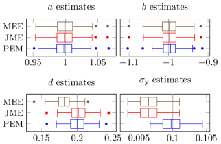
Figure 1: Boxplots of estimated parameters of the Duffing oscillator with Gaussian measurement noise. The nominal values are marked with gray vertical lines.

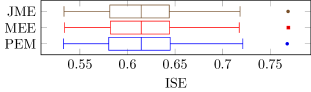
Figure 2: Boxplot of the state-path estimation error of the Duffing oscillator with Gaussian measurement noise.

In Fig. 1, boxplots of the parameter estimates of the three estimators are shown. It can be seen that the distribution of the estimates of the drift-function parameters by the JME and PEM is very similar. The MEE, on the other hand, is biased for the $d$ parameter, which represents the damping of the system. This is because the drift divergence $\operatorname{div}_{x}f(t,x,z,\theta)=-d$. Consequently, higher values for the $d$ parameter imply that the system strongly attenuates the fluctuations due to the process noise and increase the probability of small balls around the state path. The MEE, which does not take this into account, underestimates this parameter. It should also be noted that both the MEE and JME are biased for the $\sigma_{\mathrm{y}}$ parameter, as lower values of this parameter also increase the probability of small balls around state paths.

To evaluate the state-path estimation error, the integrated square error (ISE) metric was used, given by

$$\textstyle\operatorname{ISE}=\int_{0}^{T}[(X_{t}-x_{t})^{2}+(Z_{t}-z_{t})^{2}]\,\mathrm{d}t,$$ (22)

where $X$ and $Z$ are the simulated paths and $x$ and $z$ their estimates. Boxplots of the ISE distribution of the three estimators is shown in Fig. 2, in which we see that their error is comparable.

4.2 Measurements with outlier noise

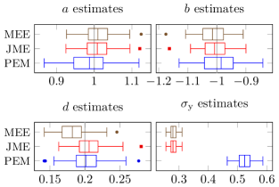
Figure 3: Boxplots of estimated parameters of the Duffing oscillator with outlier measurement noise. The nominal values are marked with gray vertical lines.

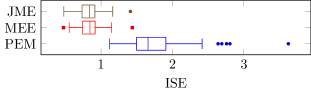
Figure 4: Boxplot of the state-path estimation error of the Duffing oscillator with outlier measurement noise.

For the second example, measurement noise with outliers was used, to illustrate the advantages of the proposed estimator for robust system identification and smoothing. Each measured value $Y_{k}$ was drawn independently from the Gaussian mixture distribution

$$Y_{k}|X,Z,\Theta\sim p_{\mathrm{o}}\mathcal{N}\!\left(Z_{kt_{\mathrm{s}}},\sigma_{\mathrm{o}}^{2}\right)+(1-p_{\mathrm{o}})\mathcal{N}\!\left(Z_{kt_{\mathrm{s}}},\sigma_{\mathrm{r}}^{2}\right),$$ (23)

where $p_{\mathrm{o}}=0.25$ is the outlier probability, $\sigma_{\mathrm{o}}=1$ is the outliers’ standard deviation, and $\sigma_{\mathrm{r}}=0.2$ is the regular measurements’ standard deviation. The total experiment length $T=100$ was used. This experiment is similar to those of Aravkin et al. (2012b) and Dutra et al. (2014).

For estimation with the MEE and JME, a measurement model different from the one used to generate the data was used in the estimation. Student’s $t$-distribution with 4 degrees of freedom and unknown scale $\Sigma_{\mathrm{y}}$ was used as the measurement likelihood, with the following expression for its log-likelihood:

$$\textstyle\ln\psi(y|x,z,\theta)=-\sum_{k=0}^{N}\left[\frac{5}{2}\ln\big{(}1+\frac{(y_{k}-z_{kt_{\mathrm{s}}})^{2}}{4\sigma_{\mathrm{y}}^{2}}\big{)}+\ln\sigma_{\mathrm{y}}\right],$$ (24)

where the constant terms have been omitted as they do not influence the location of maxima. For the estimation of $\Sigma_{\mathrm{y}}$, the gamma distribution with shape $r$ and scale $s$ was chosen as its prior, as in the previous experiment. The optimization starting point for the MEE and JME was also the same as in Sec. 4.1.

Boxplots of the parameter estimates by the three estimators are shown in Fig. 3. It can be seen that, as in the previous example, the MEE is biased for the $d$ parameter. In this experiment, however, the PEM also presents a larger interquartile range than the JME. The difference between the PEM and JME is clearer on the state-path estimation error, shown in Fig. 4. The JME and MEE achieve lower errors because the $t$-distribution fits the heavy-tailed distribution used to generate the measurements better than the Gaussian distribution which underlies the PEM and UKS. We note that no nominal value is marked for $\sigma_{\mathrm{y}}$ as a measurement model different from the one used to generate the data was used for the estimation. Furthermore, this parameter has a different meaning for the PEM and for the JME–MEE.

5 Conclusions and future work

In this paper, we extended the estimator of Dutra et al. (2014) for joint MAP and minimum-energy state-path and parameter estimation. The minimum-energy estimator is proved to estimate the joint MAP noise paths, initial states, and parameters. The difference between the MAP and minimum-energy estimators is that the former takes into account the amplification or attenuation by the system of the pertubations due to the process noise. It does so by including the drift-divergence integral in its log-posterior. Simulated experiments show that this is important for preventing the biasing of parameters related to the system’s energy-loss rate.

These results suggest that the Onsager–Machlup functional should be used instead of the energy functional in approximate MAP or maximum likelihood estimation by coestimating the state path as nuisance parameter (cf. Varziri et al., 2008). It also indicates that the Onsager–Machlup functional should be used in MAP parameter estimators which marginalize the state-path using the Laplace approximation (Karimi and McAuley, 2014), which we intend to investigate in future work.

The JME and MEE were also compared with the PEM, which occupies a similar niche of applications as its parameters are estimated as single vector and not as a time-varying signal. In the example with Gaussian noise, the drift-function parameter estimates by the JME were comparable to those by the PEM. However, one advantage of the JME is that it is applicable to systems with a wider range of measurement distributions. In the experiment with non-Gaussian measurements, the JME obtained lower errors than the PEM. One serious disadvantage of the JME, however, is that it cannot be used to estimate the diffusion matrix, unlike the PEM.

References

- Aguirre and Letellier [2009] L.A. Aguirre and C. Letellier. Modeling nonlinear dynamics and chaos: a review. Math. Probl. Eng., 2009:238960, 2009.
- Aihara and Bagchi [1999a] S.I. Aihara and A. Bagchi. On the Mortensen equation for maximum likelihood state estimation. IEEE Trans. Autom. Control, 44(10):1955–1961, 1999a.
- Aihara and Bagchi [1999b] S.I. Aihara and A. Bagchi. On maximum likelihood nonlinear filter under discrete-time observations. In IEEE ACC, volume 1, pages 450–454, 1999b.
- Arasaratnam et al. [2010] I. Arasaratnam, S. Haykin, and T.R. Hurd. Cubature Kalman filtering for continuous-discrete systems: Theory and simulations. IEEE Trans. Signal Process., 58(10):4977–4993, 2010.
- Aravkin et al. [2011] A.Y. Aravkin, B.M. Bell, J.V. Burke, and G. Pillonetto. An -Laplace robust Kalman smoother. IEEE Trans. Autom. Control, 56(12):2898–2911, 2011.
- Aravkin et al. [2012a] A.Y. Aravkin, J.V. Burke, and G. Pillonetto. Nonsmooth regression and state estimation using piecewise quadratic log-concave densities. In IEEE CDC, pages 4101–4106, 2012a.
- Aravkin et al. [2012b] A.Y. Aravkin, J.V. Burke, and G. Pillonetto. Robust and trend-following Kalman smoothers using Student’s t. In SYSID, pages 1215–1220, 2012b.
- Aravkin et al. [2012c] A.Y. Aravkin, J.V. Burke, and G. Pillonetto. A statistical and computational theory for robust and sparse Kalman smoothing. In SYSID, pages 894–899, 2012c.
- Aravkin et al. [2013] A.Y. Aravkin, J.V. Burke, and G. Pillonetto. Sparse/robust estimation and Kalman smoothing with nonsmooth log-concave densities. J. Mach. Learn. Res., 14(9):2689–2728, 2013.
- Bell et al. [2009] B.M. Bell, J.V. Burke, and G. Pillonetto. An inequality constrained nonlinear Kalman–Bucy smoother by interior point likelihood maximization. Automatica, 45(1):25–33, 2009.
- Betts [2010] J.T. Betts. Practical methods for optimal control and estimation using nonlinear programming. SIAM, 2nd edition, 2010.
- Capitaine [2000] M. Capitaine. On the Onsager–Machlup functional for elliptic diffusion processes. In Séminaire de Probabilités XXXIV, pages 313–328. Springer, 2000.
- Dutra [2014] D.A. Dutra. Maximum a posteriori joint state path and parameter estimation in stochastic differential equations. PhD thesis, UFMG, 2014. URI: http://hdl.handle.net/1843/BUOS-9S3H9D.
- Dutra et al. [2012] D.A. Dutra, B.O.S. Teixeira, and L.A. Aguirre. Joint maximum a posteriori smoother for state and parameter estimation in nonlinear dynamical systems. In SYSID, pages 900–905, 2012.
- Dutra et al. [2014] D.A. Dutra, B.O.S. Teixeira, and L.A. Aguirre. Maximum a posteriori state path estimation: Discretization limits and their interpretation. Automatica, 50(5):1360–1368, 2014.
- Farahmand et al. [2011] S. Farahmand, G.B. Giannakis, and D. Angelosante. Doubly robust smoothing of dynamical processes via outlier sparsity constraints. IEEE Trans. Signal Process., 59(10):4529–4543, 2011.
- Ghosh et al. [2008] S. J. Ghosh, C. S. Manohar, and D. Roy. A sequential importance sampling filter with a new proposal distribution for state and parameter estimation of nonlinear dynamical systems. Proc. R. Soc. A, 464(2089):25–47, 2008.
- Huber and Ronchetti [2009] P.J. Huber and E.M. Ronchetti. Robust Statistics. Wiley, 2nd edition, 2009.
- Karimi and McAuley [2014] H. Karimi and K.B. McAuley. A maximum-likelihood method for estimating parameters, stochastic disturbance intensities and measurement noise variances in nonlinear dynamic models with process disturbances. Comput. Chem. Eng., 67(4):178–198, 2014.
- Khalil et al. [2009] M. Khalil, A. Sarkar, and S. Adhikari. Nonlinear filters for chaotic oscillatory systems. Nonlinear Dynam., 55(1-2):113–137, 2009.
- Kloeden and Platen [1992] P.E. Kloeden and E. Platen. Numerical Solution of Stochastic Differential Equations. Springer, 1992.
- Kristensen et al. [2004] N.R. Kristensen, H. Madsen, and S.B. Jørgensen. Parameter estimation in stochastic grey-box models. Automatica, 40(2):225–237, 2004.
- Lange et al. [1989] K.L. Lange, R.J.A. Little, and J.M.G. Taylor. Robust statistical modeling using the t distribution. J. Amer. Statist. Assoc., 84(408):881–896, 1989.
- Levy and Nikoukhah [2013] B.C. Levy and R. Nikoukhah. Robust state space filtering under incremental model perturbations subject to a relative entropy tolerance. IEEE Trans. Autom. Control, 58(3):682–695, 2013.
- Monin [2013] A. Monin. Modal trajectory estimation using maximum Gaussian mixture. IEEE Trans. Autom. Control, 58(3):763–768, 2013.
- Namdeo and Manohar [2007] V. Namdeo and C.S. Manohar. Nonlinear structural dynamical system identification using adaptive particle filters. J. Sound and Vib., 306(3–5):524–563, 2007.
- Polak [2011] E. Polak. On the role of optimality functions in numerical optimal control. Annu. Rev. Control, 35(2):247–253, 2011.
- Särkkä [2008] S. Särkkä. Unscented Rauch–Tung–Striebel smoother. IEEE Trans. Autom. Control, 53(3):845–849, 2008.
- Takahashi and Watanabe [1981] Y. Takahashi and S. Watanabe. The probability functionals (Onsager–Machlup functions) of diffusion processes. In 19th LMS Durham Symposium, pages 433–463, 1981.
- Varziri et al. [2008] M.S. Varziri, K.B. McAuley, and P.J. McLellan. Parameter and state estimation in nonlinear stochastic continuous-time dynamic models with unknown disturbance intensity. Can. J. Chem. Eng., 86(5):828–837, 2008.
- Wächter and Biegler [2006] A. Wächter and L.T. Biegler. On the implementation of an interior-point filter line-search algorithm for large-scale nonlinear programming. Math. Program., 106(1):25–57, 2006.
- Zeitouni [1989] O. Zeitouni. On the onsager–machlup functional of diffusion processes around non curves. Ann. Probab., 17:1037–1054, 1989.
- Zeitouni and Dembo [1987] O. Zeitouni and A. Dembo. A maximum a posteriori estimator for trajectories of diffusion processes. Stochastics, 20(3):221–246, 1987.
- Zorzi [2016] Mattia Zorzi. Robust kalman filtering under model perturbations. IEEE Trans. Autom. Control, PP(99):1–6, 2016.