Period map of triple coverings of $\mathbb{P}^{2}$ and mixed Hodge structures

Abstract.

We study a period map for triple coverings of $\mathbb{P}^{2}$ branching along special configurations of $6$ lines. Though the moduli space of special configurations is a two dimensional variety, the minimal models of the coverings form a one parameter family of K3 surfaces. We extract extra one dimensional information from the mixed Hodge structure on the second relative homology group. We define the period map from the moduli space of marked configurations to the domain $\mathbb{B}\times\mathbb{C}^{2}$, where $\mathbb{B}$ is the right half plane, and give a defining equation of its image by a theta function. We write down the inverse of the period map using theta functions.

1. Introduction

1.1. Introduction

Period integrals of cyclic coverings of $\mathbb{P}^{2}$ branching along configurations of several lines satisfy a hypergeometric system of linear differential equations. In the paper [MSTY], we study several examples of reducible hypergeometric systems of differential equations. We treat a special case where the branch index is equal to $(\dfrac{1}{3},\dfrac{1}{3},\dfrac{1}{3},\dfrac{1}{3},\dfrac{1}{3},\dfrac{4}{3})$ with the notation in [MSTY] and the branching lines $\ell_{1},\dots,\ell_{6}$ satisfy the following conditions.

1. The intersection $\ell_{i}\cap\ell_{j}\cap\ell_{k}$ is a point for $(i,j,k)=(1,3,6),(2,4,6)$.

2. The intersection $\ell_{i}\cap\ell_{j}\cap\ell_{k}$ is an empty set if $1\leq i<j<k\leq 6$ and $(i,j,k)\neq(1,3,6),(2,4,6)$.

A configuration of $6$ lines $\vec{\ell}=\{\ell_{1},\dots,\ell_{6}\}$ satisfying the above condition is simply called a special configuration. By changing projective coordinates of $\mathbb{P}^{2}$, we normalize $\ell_{i}$ as

$$\ell_{1}=p,\quad\ell_{2}=q,\quad\ell_{3}=1-p,\quad\ell_{4}=1-q,$$

$$\ell_{5}=1-x_{1}p-x_{2}q,$$

and $\ell_{6}$ is the infinite line, where $p$ and $q$ are inhomogeneous coordinates of $\mathbb{P}^{2}$. We identify the moduli space $\mathcal{M}$ of special configurations of $6$ lines with

$$\{(x_{1},x_{2})\in\mathbf{C}^{2}\mid x_{1}x_{2}(x_{1}-1)(x_{2}-1)(x_{1}+x_{2}-1)\neq 0\}$$

by considering the the condition (2) for the normalized lines.

For an element $\vec{\ell}\in\mathcal{M}$, we have a branched cyclic triple covering $X=X_{\vec{\ell}}$ of $\mathbf{P}^{2}$ defined by

$$X:z^{3}=p^{-2}q^{-2}(1-p)^{-2}(1-q)^{-2}(1-x_{1}p-x_{2}q)^{-2}.$$

The period integrals of $X$ satisfy Appell’s hypergeometric system $F_{2}$ of differential equations with the parameters $(a;b_{1},b_{2};c_{1},c_{2})=(2/3;1/3,1/3;2/3,2/3)$.

In this paper, we study the period map for a family $\{X_{\vec{\ell}}\}_{\vec{\ell}\in\mathcal{M}}$.

One can see that the minimal compact smooth model $\widetilde{X}$ of $X$ is a K3 surface. Let $E_{2}$ be the divisor of $\widetilde{X}$ lying over the intersection point $\ell_{2}\cap\ell_{4}\cap\ell_{6}$. Let $\rho$ be an automorphism of $X$ defined by $(p,q,z)\mapsto(p,q,\omega z)$ where $\omega=\dfrac{-1+\mathbb{i}\sqrt{3}}{2}$. The invariant part of the relative cohomology $H_{2}(\widetilde{X},E_{2},\mathbb{Z})$ under the action of $\rho$ is denoted by $H_{2}(\widetilde{X},E_{2},\mathbb{Z})^{\rho}$. Then the quotient group

$$H_{2}(\widetilde{X},E_{2},\mathbb{Z})_{\rho}=H_{2}(\widetilde{X},E_{2},\mathbb{Z})/H_{2}(\widetilde{X},E_{2},\mathbb{Z})^{\rho}$$

becomes a free $\mathbb{Z}[\rho]$-module of rank $3$. Here $\mathbb{Z}[\rho]=\mathbb{Z}\oplus\mathbb{Z}\rho$, with the relation $\rho-2+\rho+1=0$.

By Deligne [D], $H_{2}(\widetilde{X},E_{2},\mathbb{Z})_{\rho}$ is equipped with a natural mixed Hodge structure, whose weight $(-2)$-part is identified with $H_{2}(\widetilde{X},\mathbb{Z})_{\rho}$. The module $H_{2}(\widetilde{X},\mathbb{Z})_{\rho}$ is identified with the generic transcendental part and becomes a lattice by the intersection form. In other words, the module $H_{2}(\widetilde{X},E_{2},\mathbb{Z})_{\rho}$ is equipped with the graded polarized mixed Hodge structure. In this paper, we treat the period map for the mixed Hodge structure $H_{2}(\widetilde{X},E_{2},\mathbb{Z})_{\rho}$ and its inverse map.

To formulate the period map, we define a marking (Definition 6.3) of the Hodge structure on $H_{2}(\widetilde{X},E_{2},\mathbb{Z})_{\rho}$. We introduce a standard module $W_{(-1)}=\langle B_{1},B_{2},B_{3}\rangle_{\mathbb{Z}[\rho]}$ equipped with a filtration $W_{(-2)}=\langle B_{1},B_{2}\rangle\subset W_{(-1)}$ and a symmetric bilinear form on $W_{(-2)}$. The marking of $H_{2}(\widetilde{X},E_{2},\mathbb{Z})_{\rho}$ is defined as a $\mathbb{Z}[\rho]$-isomorphism

$$\mu:W_{(-1)}\xrightarrow{\simeq}H_{2}(\widetilde{X},E_{2},\mathbb{Z})_{\rho}$$

satisfying some properties (see Definition 6.3). A marked configuration $(\overset{\to}{\ell},\mu)=((x_{1},x_{2}),\mu)$ is defined as a pair of a point $\overset{\to}{\ell}=(x_{1},x_{2})$ in $\mathcal{M}$ and a marking $\mu$ of $H_{2}(\widetilde{X},E_{2},\mathbb{Z})_{\rho}$. The moduli space of marked configurations is denoted by $\mathcal{M}_{mk}$.

We set $\mathbb{B}=\{\eta\in\mathbb{C}\mid\ \operatorname{Re}(\eta)>0\}$ and $\mathcal{D}=\mathbb{B}\times\mathbb{C}^{2}$. In §6, using the markings $\mu$ of the mixed Hodge structures, we define the period map

$$per:\mathcal{M}_{mk}\to\mathcal{D}$$

as follows. Let $\chi$ be a character of the group $\langle\rho\rangle$ generated by $\rho\in Aut(X)$ defined by $\chi(\rho)=\omega$ and its complex conjugate is denoted by $\overline{\chi}$. Then the $\chi$-part $F^{2}H^{2}_{dR,c}(\widetilde{X}-E_{2})(\chi)$ (resp. $\overline{\chi}$-part $F^{1}H^{2}_{dR,c}(\widetilde{X}-E_{2})(\overline{\chi})$) of $F^{2}H^{2}_{dR,c}(\widetilde{X}-E_{2})$ (resp. $F^{1}H^{2}_{dR,c}(\widetilde{X}-E_{2})$) is a $1$-dimensional vector space. We choose a basis $\xi$ (resp. $\overline{\xi}$) of it. Let $\langle*,*\rangle$ be the natural pairing between $H_{2}(\widetilde{X},E_{2},\mathbb{Z})_{\rho}$ and the de Rham cohomology with compact support $H^{2}_{dR,c}(\widetilde{X}-E_{2})$. We define a (unnormalized) period matrix $P((x_{1},x_{2}),\mu)$ by

$$P((x_{1},x_{2}),\mu)=\begin{pmatrix}p_{11}&p_{12}\\ p_{21}&p_{22}\\ p_{31}&p_{32}\\ \end{pmatrix},\quad p_{i1}=\langle\mu(B_{i}),\xi\rangle,p_{i2}=\langle\mu(B_{i}),\overline{\xi}\rangle.$$

For an element $((x_{1},x_{2}),\mu)\in\mathcal{M}_{mk}$, we define the period $per((x_{1},x_{2}),\mu)=(\eta,z)\in\mathcal{D}$ by ratios

$$\eta=\dfrac{p_{11}}{p_{21}},\quad z=(z_{1},z_{2})=(\frac{p_{31}}{p_{21}},\frac{p_{32}}{p_{22}})$$

of entries of the period matrix $P((x_{1},x_{2}),\mu)$. Note that the map $per$ does not depend on the choice of $\xi$ and $\overline{\xi}$.

To study the period $P((x_{1},x_{2}),\mu)$, we give two elliptic fibrations $\epsilon_{1},\epsilon_{2}$ on the K3 surface $\widetilde{X}$ in §2. The fibration $\epsilon_{1}$ (resp. $\epsilon_{2}$) is an isotrivial family with a finite monodromy group. The monodromy covering $C\to\mathbb{P}^{1}$ is defined by the minimal covering of $\mathbb{P}^{1}$ such that the fibration $\epsilon_{1}$ is trivialized by the base change by the covering map $C\to\mathbb{P}^{1}$. Then $C$ is a triple covering of $\mathbb{P}^{1}$ depending only on

$$t=\dfrac{1-x_{1}-x_{2}}{(1-x_{1})(1-x_{2})},$$

and its genus is $2$. Using the fibration $\epsilon_{1}$, we obtain a rational map $\lambda:E\times C_{t}\dashrightarrow\widetilde{X}$. The image $\epsilon_{1}(E_{2})$ of $E_{2}$ under the map $\epsilon_{1}$ is a one point and the inverse image of $\epsilon(E_{2})$ in $C$ is denoted by $\Sigma_{1}$. The rational map $\lambda$ induces an injection of mixed Hodge structures

(1.1) $$H_{1}(C,\Sigma_{1},\mathbb{Z})\otimes_{\mathbb{Z}[\rho]}H_{1}(E,\mathbb{Z})\to H_{2}(\widetilde{X},E_{2},\mathbb{Z})_{\rho}.$$

Via this map, we study the structure of the generic transcendental lattice $T_{X}$ of the K3 surface $\widetilde{X}$ in §4.

In §3, we study the relative homology $H_{1}(C,\Sigma_{1},\mathbb{Z})$. Let $H_{0}(\Sigma_{1},\mathbb{Z})^{0}$ be the kernel of the natural map $H_{0}(\Sigma_{1},\mathbb{Z})\to H_{0}(C,\mathbb{Z})$. Then $H_{0}(\Sigma_{1},\mathbb{Z})^{0}$ is a free $\mathbb{Z}[\rho]$-module generated by $(1-\rho)p_{1}$, where $p_{1}$ is an element in $\Sigma_{1}$. We have an exact sequence

(1.2) $$0\to H_{1}(C,\mathbb{Z})\to H_{1}(C,\Sigma_{1},\mathbb{Z})\to H_{0}(\Sigma_{1},\mathbb{Z})^{0}\to 0$$

arising from the weight filtration of the mixed Hodge structure on $H_{1}(C,\Sigma_{1},\mathbb{Z})$. Using the injection (1.1) and the marking $\mu$, we obtain

1. a symplectic basis $\{\alpha_{1},\alpha_{2},\beta_{1},\beta_{2}\}$ of $H_{1}(C,\mathbb{Z})$ satisfying $\alpha_{1}=\rho(\beta_{2}),\alpha_{2}=\rho(\beta_{1})$, and

2. a lifting $\beta_{3}$ of $(1-\rho)p_{1}$ in $H_{1}(C,\Sigma_{1},\mathbb{Z})$.

Let $F^{1}H^{1}_{dR,c}(C-\Sigma_{1})$ be the first Hodge filtration in $H^{1}_{dR,c}(C-\Sigma_{1})$. Via the exact sequence (1.2), we have an isomorphism for the Hodge filtrations

$$F^{1}H^{1}_{dR,c}(C-\Sigma_{1})\simeq F^{1}H^{0}_{dR}(C)=H^{0}(C,{\it\Omega}^{1}_{C}).$$

Let $\psi_{1}^{\prime},\psi_{2}^{\prime}$ be the basis of $H^{0}(C,{\it\Omega}^{1}_{C})$ normalized by $\displaystyle\langle\beta_{i},\psi_{j}^{\prime}\rangle=\delta_{ij},$ where $\langle*,*\rangle$ is the natural pairing between $H_{1}(C,\Sigma_{1},\mathbb{Z})$ and $H^{1}_{dR,c}(C-\Sigma_{1})$. We define the normalized period matrix $\tau\in M(2,\mathbb{C})$ of $C$ and incomplete integrals $\zeta\in\mathbb{C}^{2}$ by

$$\tau=\begin{pmatrix}\langle\alpha_{1},\psi^{\prime}_{1}\rangle,\langle\alpha_{1},\psi^{\prime}_{2}\rangle\\ \langle\alpha_{2},\psi^{\prime}_{1}\rangle,\langle\alpha_{2},\psi^{\prime}_{2}\rangle\\ \end{pmatrix},\quad\zeta=\begin{pmatrix}\langle\dfrac{\beta_{3}}{1-\rho},\psi^{\prime}_{1}\rangle,\langle\dfrac{\beta_{3}}{1-\rho},\psi^{\prime}_{2}\rangle\\ \end{pmatrix}.$$

Then $\tau$ belongs to the Siegel upper half space $\mathbb{H}_{2}=\{\tau\in M_{2}(\mathbb{C})\mid\tau=\ ^{t}\tau,\operatorname{Im}(\tau)>0\}$ and the class of $\zeta$ is in the image of Abel-Jacobi map $C\to J(C)=\mathbb{C}^{2}/(\mathbb{Z}^{2}\tau+\mathbb{Z}^{2})$. Using the fact that the injection (1.1) is a homomorphism of mixed Hodge structures with an action of $\rho$, we can express $\tau$ and $\zeta$ as

(1.3) $$\tau =\frac{1}{2}\begin{pmatrix}\sqrt{-3}\eta^{-1}&-1\\ -1&\sqrt{-3}\eta\\ \end{pmatrix},$$

$$\zeta =\frac{1}{2}\left((\dfrac{z_{1}}{1-\omega}-\dfrac{z_{2}}{1-\omega^{2}})\eta^{-1},\dfrac{z_{1}}{1-\omega}+\dfrac{z_{2}}{1-\omega^{2}}\right),$$

where $per((x_{1},x_{2}),\mu)=(\eta,z_{1},z_{2})$.

For an element $(x_{1},x_{2})\in\mathcal{M}$ satisfying the conditions $x_{1},x_{2}\in\mathbb{R},0<x_{1},0<x_{2},x_{1}+x_{2}<1$, we define explicit relative topological 2-cycles $\Gamma_{1},\Gamma_{2},\Gamma_{3}$ and $\Gamma_{4}$ of $H_{2}(\widetilde{X},E_{1}\cup E_{2},\mathbb{Z})$ in §5.1. Using these topological 2-cycles, we define a marking $\mu$ in Example 6.6.2. For this marking $\mu$ and a suitable choice of $\xi,\overline{\xi}$, the pairings $\langle\mu(B_{i}),\xi\rangle$ and $\langle\mu(B_{i}),\overline{\xi}\rangle$ are expressed in terms of hypergeometric integrals (5.2).

Let $\Gamma$ be the unitary group with the coefficients in $\mathbb{Z}[\rho]$ for the hermitian matrix $U=\begin{pmatrix}0&1\\ 1&0\end{pmatrix}$, and let $G=\Gamma\ltimes\mathbb{Z}[\rho]^{2}$ be the semi-direct product of $\Gamma$ and $\mathbb{Z}[\rho]^{2}$ obtained by the standard right action of $\Gamma$ on $\mathbb{Z}[\rho]^{2}$. Then the group $G$ is identified with a subgroup of $GL(3,\mathbb{Z}[\rho])$. Its principal congruence subgroup of level $(1-\rho)$ is denoted by $G(1-\rho)$. Then the group $G(1-\rho)$ acts on the moduli space $\mathcal{M}_{mk}$ by the action on the set of markings. Using the relation (1.3), we define an embedding $\jmath_{\mathcal{D}}:\mathbb{B}\times\mathbb{C}^{2}\to\mathbb{H}_{2}\times\mathbb{C}^{2}$ by $\jmath_{\mathcal{D}}(\eta,z)=(\tau,\zeta)$, which is equivariant under the group homomorphism $\jmath_{G}:G(1-\rho)\to Sp_{2}(\mathbb{Z})\ltimes\mathbb{Z}^{4}$.

In §7, we prove that the image $per(\mathcal{M}_{mk})\subset\mathcal{D}$ under the period map is a codimension one complex analytic space $V(\vartheta)$ defined by the zero locus of a theta function $\vartheta$ for the period matrix $\tau$. As a consequence, we have an isomorphism

$$\mathcal{M}\simeq V(\vartheta)/G(1-\rho)\subset\mathcal{D}/G(1-\rho).$$

By using the embedding $\jmath_{\mathcal{D}}$ and theta functions on $\mathbf{H}_{2}\times\mathbf{C}^{2}$ with characteristics, we give the inverse of the above isomorphism $\overline{per}:\mathcal{M}\to V(\vartheta)/G(1-\rho)$.

1.2. Notations

1. Let $\mathbb{Z}[\rho]$ be a commutative ring generated by $\rho$ with a relation $\rho^{2}+\rho+1=0$. The conjugate map $\overline{\ }:\mathbb{Z}[\rho]\to\mathbb{Z}[\rho]$ is the ring homomorphism defined by $\overline{\rho}=\rho^{-1}=-1-\rho$. We set

   $$\operatorname{Re}:\mathbb{Z}[\rho]\ni x\mapsto\dfrac{x+\overline{x}}{2}\in\dfrac{1}{2}\mathbb{Z}.$$

2. Let $\chi$ be a character of the cyclic group $\langle\rho\rangle$ of order three. For a $\mathbb{C}$-vector space $V_{\mathbb{C}}$ with an action of $\langle\rho\rangle$, $V_{\mathbb{C}}(\chi)$ denotes the $\chi$-part

   $$V_{\mathbb{C}}(\chi)=\{v\in V_{\mathbb{C}}\mid\rho(v)=\chi(\rho)v\}.$$

   of $V_{\mathbb{C}}$. For the conjugate character $\overline{\chi}$, $V_{\mathbf{C}}(\overline{\chi})$ denotes the $\overline{\chi}$-part of $V_{\mathbf{C}}$.

3. For a module $M$ with an action of $\rho$, $M^{\rho}$ and $M_{\rho}$ denote the $\rho$-invariant part and the $\rho$-coinvariant part $M_{\rho}=M/M^{\rho}$ of $M$, respectively. Then $M_{\rho}$ becomes a $\mathbb{Z}[\rho]$-module.

4. For a topological space $X$ (resp. a pair of topological spaces $X\supset Y$), the $i$-th singular cohomology and homology (resp. relative homology) with integral coefficients are denoted by $H^{i}(X)$ and $H_{i}(X)$ (resp. $H_{i}(X,Y)$). The $i$-th de Rham cohomology (resp. de Rham cohomology with compact support) of an algebraic variety is denoted by $H_{dR}^{i}(X)$ (resp. $H_{dR,c}^{i}(X)$). It is a $\mathbb{C}$-vector space.

5. In this paper, a lattice means a finitely generated free $\mathbb{Z}$-module with a symmetric bilinear form over $\mathbb{Q}$. For a lattice $(L,\langle\ ,\ \rangle)$, $L(m)$ denotes a lattice $(L,m\langle\ ,\ \rangle)$ i.e. the module $L$ with the symmetric bilinear form $m\langle\ ,\ \rangle$.

1.3. Acknowledgment

The study of period integrals of open K3 surfaces is motivated by the previous work [MSTY] on reducible hypergeometric equation. The authors express their gratitude to T. Sasaki and M. Yoshida for discussions with them.

2. Triple covering of $\mathbb{P}^{2}$ branching along special configuration of $6$ lines

2.1. Moduli spaces of special configurations

In this subsection, we define a triple covering $X$ of $\mathbb{P}^{2}$ branching along a special configuration of 6 lines.

Two numbered sets of $6$ lines $(\ell_{1},\cdots,\ell_{6})$ and $(\ell_{1}^{\prime},\cdots,\ell_{6}^{\prime})$ in $\mathbb{P}^{2}$ are projectively equivalent, if and only if there exists an element $g$ in $PGL_{3}(\mathbb{C})$ such that $\ell_{i}=g(\ell_{i}^{\prime})$ for $i=1,\dots,6$.

Definition 2.1.

A numbered set of $6$ lines $\vec{\ell}=(\ell_{1},\dots,\ell_{6})$ in $\mathbb{P}^{2}$ is called a special configuration, if it satisfies the following conditions:

1. the intersection $\ell_{i}\cap\ell_{j}\cap\ell_{k}$ is a point, if $(i,j,k)=(1,3,6),(2,4,6)$,

2. $\ell_{i}\cap\ell_{j}\cap\ell_{k}=\emptyset$, if $1\leq i<j<k\leq 6$, $(i,j,k)\neq(1,3,6),(2,4,6)$.

The set of projective equivalence classes of special configurations is denoted by $\mathcal{M}$.

We can choose an inhomogeneous coordinates $(p,q)$ of $\mathbb{P}^{2}$ so that $\ell_{6}$ is the line at infinity. We use the same notation $\ell_{i}$ for the equation of the line $\ell_{i}$. We choose an inhomogeneous coordinate $(p,q)$ so that the defining equations are given by

$$\ell_{1}=p,\quad\ell_{2}=q,\quad\ell_{3}=1-p,\quad\ell_{4}=1-q,$$

$$\ell_{5}=1-x_{1}p-x_{2}q.$$

Under the above normalization, we have the following identification:

$$\mathcal{M}=\{(x_{1},x_{2})\in\mathbb{C}^{2}\mid x_{1},x_{2}\neq 0,1,\ x_{1}+x_{2}\neq 1\}.$$

For an element $\vec{\ell}\in\mathcal{M}$, we define a cyclic triple covering

$$\pi:X\to\mathbb{P}^{2}$$

branching along the $6$ lines $\ell_{1},\dots,\ell_{6}$ by

(2.1) $$X=X_{\vec{\ell}}:z^{3}=p^{-2}q^{-2}(1-p)^{-2}(1-q)^{-2}(1-x_{1}p-x_{2}q)^{-2}.$$

The ramification divisor of $\pi$ is given by $D=\cup_{i=1}^{6}\pi^{-1}(\ell_{i}).$

2.2. K3 surfaces obtained by triple coverings and Picard lattices

Let $\overset{\to}{\ell}$ be a configuration in $\mathcal{M}$ and set $p_{1}=\ell_{1}\cap\ell_{3}\cap\ell_{6}$, $p_{2}=\ell_{2}\cap\ell_{4}\cap\ell_{6}$. The blowing up of $\mathbb{P}^{2}$ with centers $p_{1},p_{2}$ is denoted by $\widehat{\mathbb{P}^{2}}$ (see Figure 1). The exceptional divisors over $p_{1}$ and $p_{2}$ are denoted by $e_{1}$ and $e_{2}$. The pencil with the axis $p_{1}$ (resp. $p_{2}$) defines a morphism $\overline{\epsilon_{1}}:\widehat{\mathbb{P}^{2}}\to\mathbb{P}^{1}$ which is expressed as

$$\overline{\epsilon_{1}}:(p,q)\mapsto p\quad(\text{resp. }\overline{\epsilon_{2}}:(p,q)\mapsto q)$$

by the inhomogeneous coordinates $(p,q)$ of $\mathbb{P}^{2}$. The morphism

$$\widehat{\mathbb{P}^{2}}\xrightarrow{(\overline{\epsilon_{1}},\overline{\epsilon_{2}})}\mathbb{P}^{1}\times\mathbb{P}^{1}$$

is identified with the contraction of the proper transform of the line $\ell_{6}$ in $\widehat{\mathbb{P}^{2}}$. The images of $e_{1},e_{2}$ and $\ell_{1},\dots,\ell_{5}$ under the contraction $\widehat{\mathbb{P}^{2}}\to\mathbb{P}^{1}\times\mathbb{P}^{1}$ are also denoted by $e_{1},e_{2}$ and $\ell_{1},\dots,\ell_{5}$.

Figure 1. Birational transform

Let $\pi^{\prime}:X^{\prime}\to\mathbb{P}^{1}\times\mathbb{P}^{1}$ be the normalization of $X$ over $\mathbb{P}^{1}\times\mathbb{P}^{1}$. The branch locus of $\pi^{\prime}$ is the normal crossing divisor $\ell_{1}\cup\ell_{2}\cup\ell_{3}\cup\ell_{4}\cup\ell_{5}$. For $i=1,2$, the composite

$$\epsilon_{i}=\overline{\epsilon_{i}}\circ\pi:X^{\prime}\to\mathbb{P}^{1}$$

is an elliptic fibration. We set

$${\pi^{\prime}}^{-1}(e_{i})=E_{i},\ (i=1,2),\quad L_{i}={\pi^{\prime}}^{-1}(\ell_{i})\ (i=1,\dots,5),$$

and $R^{\prime}=\cup_{i=1}^{5}L_{i},D^{\prime}=R^{\prime}\cup E_{1}\cup E_{2}$. Under the map $\epsilon_{1}$ (resp. $\epsilon_{2}$), the images of the curves $L_{1},L_{3},E_{2}$ (resp. $L_{2},L_{4},E_{1}$) are points, which are denoted by $q_{1},q_{3}$ and $\sigma_{2}$ (resp. $q_{2},q_{4}$ and $\sigma_{1}$). Then we have the following diagram:

$$\begin{matrix}&X^{\prime}&\xrightarrow{\epsilon_{2}}&\mathbb{P}^{1}&\ni q_{2},q_{4},\sigma_{1}\\ &{\text{\scriptsize$\epsilon_{1}$}}\downarrow\phantom{\epsilon_{1}}&\\ q_{1},q_{3},\sigma_{2}\in&\mathbb{P}^{1},\end{matrix}$$

and an isomorphism $X^{\prime}-D^{\prime}\xrightarrow{\simeq}X-D.$

We show that the minimal resolution $\widetilde{X}$ of $X^{\prime}$ is a K3 surface. The $8$ points in $X^{\prime}$ over the intersection points in $\ell_{1}\cup\ell_{2}\cup\ell_{3}\cup\ell_{4}\cup\ell_{5}$ are $A_{2}$-singular points on $X^{\prime}$, and by the ramification formula, $\widetilde{X}$ is a K3 surface. For any $\vec{\ell}\in\mathcal{M}$, the Picard group contains the classes of $16$ exceptional divisors arising from $8A_{2}$ singularities and the classes of $E_{1},E_{2}$. Therefore the Picard number of $\widetilde{X}$ is at least $18$. The dimension of $H^{2}(X^{\prime},\mathbb{Q})$ is equal to $22-16=6$.

Definition 2.2 (Generic Neron-Severi lattice and generic transcendental lattice).

Let $\widetilde{X}$ be the minimal resolution of $X^{\prime}$.

1. We define the generic Neron-Severi lattice $S_{X}$ of $\widetilde{X}$ as the primitive closure in $H^{2}(\widetilde{X})$ of the submodule generated by

   1. the classes of $E_{1}$, $E_{2}$;

   2. the classes of $16$ exceptional divisors arising from the $8A_{2}$-singular points.

   The rank of $S_{X}$ is $18$.

2. We define the generic transcendental lattice $T_{X}$ of $\widetilde{X}$ as the orthogonal complement of $S_{X}$ in $H^{2}(\widetilde{X})$. The rank of $T_{X}$ is $4$.

3. Symmetric bilinear forms on $S_{X}$ and $T_{X}$ obtained by the intersection form on $H^{2}(\widetilde{X})$ are denoted by $\langle\ ,\ \rangle_{S}$ and $\langle\ ,\ \rangle_{T}$, respectively. Then $S_{X}$, $T_{X}$ become primitive lattices in $H^{2}(\widetilde{X})$.

2.3. The elliptic fibration $\epsilon_{1}$ and the discriminants of lattices

The elliptic fibration $\widetilde{X}\to\mathbb{P}^{1}$ obtained by $\epsilon_{1}$ is also denoted by $\epsilon_{1}$. We compute the discriminant of $S_{X}$ using the fibration $\epsilon_{1}$. For $i=1,\dots,5$, the proper transform of $L_{i}\subset X^{\prime}$ in $\widetilde{X}$ is also denoted by $L_{i}$. We set $\widetilde{R}=\cup_{i=1}^{5}L_{i}\cup E_{1}\cup E_{2}$.

Proposition 2.3.

1. The discriminant $\delta(S_{X})$ of the generic Neron-Severi lattice is equal to $9$. As a consequence, the discriminant $\delta(T_{X})$ of the generic transcendental lattice is equal to $9$.

2. The image of $H_{c}^{2}(\widetilde{X}-\widetilde{R})\to H^{2}(\widetilde{X})$ is identified with $T_{X}$. By the Poincaré duality, the image of $H_{2}(\widetilde{X})\to H_{2}(\widetilde{X},\widetilde{R})$ is identified with the dual module $T_{X}^{*}$ of $T_{X}$.

Proof.

(1) The generic fiber of the elliptic fibration $\epsilon_{1}:\widetilde{X}\to\mathbb{P}^{1}$ is an elliptic curve $E$ over the rational function field $K$ of $\mathbb{P}^{1}$. The rank of Mordell-Weil group generated by $S_{X}$ is equal to zero. Using the fact that the generic fiber of $\epsilon_{1}$ has a $\mathbb{Z}[\omega]$-multiplication, we can show

$$E(K)_{tor}\simeq(\mathbb{Z}/3\mathbb{Z}).$$

Let $V$ be the sublattice of $S_{X}$ generated by components of singular fibers, a generic fiber and the zero section. Since the type of singular fibers are $2A_{2}+2E_{6}$, $V^{*}/V$ is isomorphic to $(\mathbb{Z}/3\mathbb{Z})^{4}$. By the formula $E(K)_{tor}\simeq S_{X}/V$ due to Shioda ([S]), we have $S_{X}^{*}/S_{X}\simeq(\mathbb{Z}/3\mathbb{Z})^{2}$. Therefore $\delta(S_{X})=9$ and as a consequence, we have $\delta(T_{X})=9$.

(2) The first statement follows from the exact sequence for cohomologies

$$H^{2}_{c}(\widetilde{X}-\widetilde{R})\to H^{2}(\widetilde{X})\xrightarrow{f}H^{2}(\widetilde{R}),$$

where $f$ is obtained by the intersections with irreducible components of $\widetilde{R}$. The second statement follows from the Poincaré duality and the first statement. ∎

2.4. A trivialization by the monodromy covering

Let $t$ be an element in $\mathbb{C}-\{0,1\}$, and $C$ and $E$ be triple coverings of $\mathbb{P}^{1}$ defined by

(2.2) $$C:w^{3}=u(1-u)^{2}(1-tu)^{-1},$$

$$E:{w^{\prime}}^{3}=r^{-2}(1-r)^{-2}.$$

In this subsection, we define a rational map

$$\lambda:E\times C\dashrightarrow X^{\prime}.$$

Before defining the rational map $\lambda$, we define two birational maps $f$ and $f^{\prime}$ from $\mathbb{C}^{2}$ to itself.

1. We define a birational map $f$ by

   (2.3) $$f:(p,r)\mapsto(p,q)=(p,\dfrac{(1-x_{1}p)r}{rx_{2}-x_{2}+1-x_{1}p}).$$

   Then the rational map $f$ preserves the structure of the fibration arising from the first projection. The proper transform of $\ell_{2},\ell_{4}$ and $\ell_{5}$ are defined by $r=0,1$ and $\infty$, respectively.

2. We define the birational map $f^{\prime}$ by

   (2.4) $$f^{\prime}:(u,r)\mapsto(p,r)=(\dfrac{-u}{1-x_{1}-u},r).$$

Then the correspondence of the variables $p$ and $u$ are given by the following table,

$$\begin{array}[]{|c||c|c|c|c|c|}\hline\cr u&0&1-x_{1}&1&\dfrac{1}{t}&\infty\\[8.53581pt] \hline\cr p&0&\infty&\dfrac{1}{x_{1}}&\dfrac{1-x_{2}}{x_{1}}&1\\[8.53581pt] \hline\cr\text{fiber of }\epsilon_{1}&L_{1}&E_{2}&&&L_{3}\\[2.84526pt] \hline\cr\end{array}$$

where

(2.5) $$t=\dfrac{1-x_{1}-x_{2}}{(1-x_{1})(1-x_{2})}$$

is the cross-ratio of the four points $r_{1},r_{2},r_{3},r_{4}$ on the line $\ell_{5}$ (see Figure 1). We can easily see that via the birational map $f\circ f^{\prime}$, the open set

$$(\mathbb{P}^{1}-\{0,1,\infty\})\times(\mathbb{P}^{1}-\{0,1,\infty,\dfrac{1}{t}\})\subset\mathbb{P}^{1}\times\mathbb{P}^{1}=\{(r,u)\}$$

is mapped isomorphically onto the open set

$$\mathbb{U}=\{(p,q)\in\mathbb{P}^{1}\times\mathbb{P}^{1}\mid(p,q)\notin(\ell_{1}\cup\ell_{2}\cup\ell_{3}\cup\ell_{4}\cup\ell_{5}),p\neq\dfrac{1}{x_{1}},\dfrac{1-x_{2}}{x_{1}}\}.$$

We set

$$R_{C}=\{(w,u)\mid u=0,1,\infty,\dfrac{1}{t}\}\subset C,\quad C^{0}=C-R_{C},$$

$$R_{E}=\{(w^{\prime},r)\mid r=0,1,\infty\}\subset E,\quad E^{0}=E-R_{E},$$

$${X^{\prime}}^{0}={\pi^{\prime}}^{-1}(\mathbb{U}).$$

A covering transformation $\rho$ (resp. $\rho^{\prime}$) of $C$ (resp. $E$) over $\mathbb{P}^{1}$ is defined by $w\to\omega w$ (resp. $w^{\prime}\mapsto\omega w^{\prime}$). In the next proposition, we choose a branch of $(1-x_{1})^{\frac{1}{3}}(1-x_{2})^{\frac{1}{3}}$.

Proposition 2.4.

1. We have a morphism $\lambda:E^{0}\times C^{0}\to{X^{\prime}}^{0}$ defined by

   (2.6) $$\begin{array}[]{ccc}\lambda:E^{0}\times C^{0}&\to&{X^{\prime}}^{0}\\ ((w^{\prime},r),(w,u))&\mapsto&(z,p,q)\\[5.69054pt] &&=(\dfrac{(1-x_{1})^{\frac{2}{3}}(1-x_{2})^{\frac{2}{3}}(1-r)(1-tu)ww^{\prime}}{u(1-u)(1-p)(1-q)(1-x_{1}p-x_{2}q)},p,q).\end{array}$$

   Here $p=p(r,u),q=q(r,u)$ are rational functions on $r$ and $u$ obtained by the relations (2.3) and (2.4).

2. We define an action $\hat{\rho}$ on $E\times C$ by

   $$\hat{\rho}={\rho^{\prime}}^{-1}\times\rho.$$

   The morphism $\lambda$ factors through the quotient by the action of $\hat{\rho}$

   $$E^{0}\times C^{0}\to(E^{0}\times C^{0})/\langle\hat{\rho}\rangle,$$

   and induces an isomorphism

   (2.7) $$(E^{0}\times C^{0})/\langle\hat{\rho}\rangle\to{X^{\prime}}^{0}.$$

Proof.

The actions of $\rho$ and $\rho^{\prime}$ are fixed point free on $C^{0}$ and $E^{0}$. Since the product $ww^{\prime}$ is invariant under the action of $\hat{\rho}$, we have the statement (2). The above proposition can be checked directly from the morphism (2.6). ∎

Definition 2.5 (Monodromy covering, monodromy curve).

The covering $C\to\mathbb{P}^{1}$ is the smallest unramified covering of $\mathbb{P}^{1}-\{0,1,\infty,\dfrac{1}{t}\}$ trivializing the elliptic fibration $\epsilon_{1}:\widetilde{X}\to\mathbb{P}^{1}$. This map is called the monodromy covering and the curve $C$ is called the monodromy curve of the elliptic fibration $\epsilon_{1}:\widetilde{X}\to\mathbb{P}^{1}$.

3. Period integrals of the monodromy curve

In this section, we study period integrals of the monodromy curve $C$ defined in (2.2). Throughout this section, we assume that the parameter $t$ in (2.5) is a real number and satisfies $0<t<1$.

3.1. The homology of the monodromy curve

In this subsection, we study the structure of $H_{1}(C,\mathbb{Z})$ as $\mathbb{Z}[\rho]$-module and its intersection form. We define a symplectic basis $\alpha_{1},\alpha_{2},\beta_{1}$ and $\beta_{2}$ in the homology of $C$ as follows. We set $\beta_{1},\beta_{2}$ as in the Figure 2.

Figure 2. Cycles $\beta_{1}$ and $\beta_{2}$

The first sheet is defined so that $w$ takes a value in $\mathbb{R}_{+}$ for $0<u<1$. Paths in the first sheet are written by solid lines. Then the cycles

(3.1) $$\alpha_{1}=\rho(\beta_{2}),\ \alpha_{2}=\rho(\beta_{1}),\ \beta_{1},\ \beta_{2}$$

form a symplectic basis of the first homology $H_{1}(C,\mathbf{Z})$ of $C$; i.e, they satisfy

$$\alpha_{i}\cdot\alpha_{j}=\beta_{i}\cdot\beta_{j}=0,\quad\beta_{i}\cdot\alpha_{j}=\delta_{ij}$$

for $1\leq i,j\leq 2$, where $\delta_{ij}$ is the Kronecker symbol. We set

(3.2) $$I=\left(\begin{matrix}1&0\\ 0&1\end{matrix}\right),\quad U=\left(\begin{matrix}0&1\\ 1&0\end{matrix}\right).$$

The covering transformation $\rho$ induces a linear transformation of $H_{1}(C,\mathbf{Z})$ expressed as

$$\rho\begin{pmatrix}\alpha\\ \beta\end{pmatrix}\mapsto R\begin{pmatrix}\alpha\\ \beta\end{pmatrix},\quad\text{ where }R=\begin{pmatrix}-I&-U\\ U&O\end{pmatrix},\alpha=\begin{pmatrix}\alpha_{1}\\ \alpha_{2}\end{pmatrix},\beta=\begin{pmatrix}\beta_{1}\\ \beta_{2}\end{pmatrix}.$$

Let $E$ be the elliptic curve defined in (2.2). We define a chain $\delta_{E}$ with the positive direction in $E$ by $0\leq r\leq 1,w^{\prime}\in\mathbb{R}_{+}$ and set

$$\Delta_{E}=(1-\rho^{\prime})\delta_{E}.$$

Then $\Delta_{E}$ becomes a cycle in $E$, and $H_{1}(E,\mathbb{Z})$ is a free $\mathbb{Z}[\rho^{\prime}]$-module of rank one generated by the homology class of $\Delta_{E}$. Using the Poincaré duality, we have the following proposition.

Proposition 3.1.

We have $H^{1}(C,\mathbb{Z})=\mathbb{Z}[\rho]\beta_{1}\oplus\mathbb{Z}[\rho]\beta_{2}$ and $H^{1}(E,\mathbb{Z})=\mathbb{Z}[\rho^{\prime}]\Delta_{E}$. The intersection form is written as

(3.3) $$\langle m,n\rangle_{C} =\dfrac{2}{3}\operatorname{Re}((\rho-\overline{\rho})\ mU^{t}\overline{n}),$$

$$\langle m^{\prime},n^{\prime}\rangle_{E} =\dfrac{2}{3}\operatorname{Re}((\rho^{\prime}-\overline{\rho^{\prime}})\ m^{\prime}\overline{n^{\prime}}),$$

where the identification $m=(m_{1},m_{2})$ (resp. $m^{\prime}=(m^{\prime}_{1})$) is given by $m=m_{1}\beta_{1}+m_{2}\beta_{2}$ (resp. $m^{\prime}=m_{1}^{\prime}\Delta_{E}$) with $m_{1},m_{2}\in\mathbb{Z}[\rho]$ (resp. $m^{\prime}_{1}\in\mathbb{Z}[\rho^{\prime}]$).

3.2. Extra involution

We define an extra involution on $C=C_{t}$ for $0<t<1$.

Definition 3.2 (Extra involution).

Let $(1-t)^{1/3}$ be the positive real cubic root of $(1-t)$. We define an involution $\iota_{C}:C\to C$, called the extra involution of $C$, by setting

$$\iota_{C}^{*}(u) =\frac{1-u}{1-tu},\quad\iota_{C}^{*}(w)=(1-t)^{1/3}\frac{u(1-u)}{w(1-tu)}.$$

This involution induces a transposition of branching points and boundaries as

$$0\leftrightarrow 1,\quad\frac{1}{t}\leftrightarrow\infty,\quad 1-x_{1}\leftrightarrow 1-x_{2},$$

on the $u$-coordinate. Note that the fiber of $\epsilon_{1}$ at $u=1-x_{1}$ is a smooth elliptic curve $E_{2}$ in $\widetilde{X}$. We have a relation $\rho\circ\iota_{C}=\iota_{C}\circ\rho^{2}$.

Let $\psi_{1}$ be a holomorphic $1$-form on $C$ defined by

$$\psi_{1}=\frac{w}{u(1-u)}du=u^{-2/3}(1-u)^{-1/3}(1-tu)^{-1/3}du,$$

and $\psi_{2}$ be $\iota_{C}^{*}(\psi_{1})$. Then we have

(3.4) $$\rho^{*}(\psi_{1})=\chi(\rho)\psi_{1},\quad\rho^{*}(\psi_{2})=\overline{\chi}(\rho)\psi_{2},$$

and

$$H^{0}(C,{\it\Omega}^{1}_{C})(\chi)=\psi_{1}\mathbb{C},\quad H^{0}(C,{\it\Omega}^{1}_{C})(\overline{\chi})=\psi_{2}\mathbb{C}.$$

We set

(3.5) $$\Sigma_{i}=\{(w,u)\in C\ |\ u=1-x_{i}\},\quad(i=1,2).$$

Since the extra involution preserves the set $\Sigma_{1}\cup\Sigma_{2}$, it acts on the relative homology $H_{1}(C,\Sigma_{1}\cup\Sigma_{2})$. We define $\beta_{3}$ and $\beta_{4}$ by the following equalities:

(3.6) $$\rho(1-\rho)l_{1-x_{1}}=\beta_{3},\quad\rho(1-\rho^{2})l_{1-x_{2}}=\beta_{4}+\rho\beta_{1},$$

where $l_{1-x_{1}}$ and $l_{1-x_{2}}$ are paths in the first sheet from $(u,w)=(0,0)$ to the point with $u=1-x_{1}$ and that with $u=1-x_{2}$, respectively.

Proposition 3.3.

1. The images of $\beta_{i}$ under the extra involution $\iota_{C}$ are given as follows:

   $$\iota_{C}(\beta_{1})=\beta_{1},\quad\iota_{C}(\beta_{2})=-\beta_{2},\quad\iota_{C}(\beta_{3})=\beta_{4},\quad\iota_{C}(\beta_{4})=\beta_{3}.$$

2. We set

   (3.7) $$y_{i}=\int_{\beta_{i}}\psi_{1}\quad(i=1,\dots,4).$$

   Then

   $$\int_{\beta_{1}}\psi_{2}=y_{1},\quad\int_{\beta_{2}}\psi_{2}=-y_{2},\quad\int_{\beta_{3}}\psi_{2}=y_{4},\quad\int_{\beta_{4}}\psi_{2}=y_{3}.$$

Proof.

(1) The identities in the first statement follows from direct computations.

(2) By the definition of $\psi_{2}$, we have

$$\int_{\beta_{i}}\psi_{2}=\int_{\beta_{i}}\imath_{C}^{*}(\psi_{1})=\int_{\imath_{C*}(\beta_{i})}\psi_{1}.$$

Thus the statements follows from the results in (1). ∎

3.3. Period integral and incomplete integral on the monodromy curve

We compute the normalized period matrix of the curve $C$ in

$$\mathbb{H}_{2}=\{\tau\in M_{2}(\mathbb{C})\mid\ ^{t}\tau=\tau,\quad\operatorname{Im}(\tau)>0\}$$

with respect to the symplectic base $\alpha_{1},\dots,\beta_{2}$ defined in §3.1 using the result of the last subsection. We have

$$\left(\begin{matrix}\int_{\beta_{1}}\psi_{1}&\int_{\beta_{1}}\psi_{2}\\ \int_{\beta_{2}}\psi_{1}&\int_{\beta_{2}}\psi_{2}\\ \end{matrix}\right)=\tau_{B}=\begin{pmatrix}y_{1}&y_{1}\\ y_{2}&-y_{2}\end{pmatrix}$$

by Proposition 3.3, and

$$\left(\begin{matrix}\int_{\alpha_{1}}\psi_{1}&\int_{\alpha_{1}}\psi_{2}\\ \int_{\alpha_{2}}\psi_{1}&\int_{\alpha_{2}}\psi_{2}\\ \end{matrix}\right)=\tau_{A}=\begin{pmatrix}\omega y_{2}&-\omega^{2}y_{2}\\ \omega y_{1}&\omega^{2}y_{1}\end{pmatrix}$$

by the relations (3.1) and (3.4). The normalized period matrix $\tau=\tau_{A}\tau_{B}^{-1}$ is equal to

(3.8) $$\tau=\frac{1}{2}\begin{pmatrix}\sqrt{-3}\eta^{-1}&-1\\ -1&\sqrt{-3}\eta\\ \end{pmatrix},\quad\eta=\dfrac{y_{1}}{y_{2}}\in\mathbb{C}.$$

Note that $\tau\in\mathbf{H}_{2}$ if and only if $\eta$ is an element in

(3.9) $$\mathbb{B}=\{\eta\in\mathbb{C}\mid\operatorname{Re}(\eta)>0\}.$$

Remark 3.4.

Since $y_{1}$ and $y_{2}$ satisfies the hypergeometric geometric equation with the parameters $(a,b;c)=(1/3,1/3,1)$, the (multivalued) function $\eta$ of $t$ yields the Schwartz map with the Schwartz triangle $(3,\infty,\infty)$ (cf. [MSTY]).

We define $\delta_{3},\delta_{4}$ in $H_{1}(C,\Sigma_{1}\cup\Sigma_{2};\mathbb{Q})$ by the relations

$$(1-\rho)\delta_{3}=\beta_{3},\quad(1-\rho)\delta_{4}=\beta_{4}.$$

Then the incomplete integrals of $(\psi_{1},\psi_{2})$ along the path in the second sheet from $P_{0}$ to the point with $u=1-x_{1}$ are expressed as

(3.10) $$\bigg{(}\int_{\delta_{3}}\psi_{1},\int_{\delta_{3}}\psi_{2}\bigg{)}=\bigg{(}\dfrac{1}{1-\omega}y_{3},\dfrac{1}{1-\omega^{2}}y_{4}\bigg{)}.$$

Therefore the incomplete integrals for the normalized differential forms are equal to

(3.11) $$\zeta= \left(\dfrac{1}{1-\omega}y_{3},\dfrac{1}{1-\omega^{2}}y_{4}\right)\tau_{B}^{-1}$$

$$= \frac{1}{2}\left(\frac{y_{3}}{(1-\omega)y_{1}}+\frac{y_{4}}{(1-\omega^{2})y_{1}},\frac{y_{3}}{(1-\omega)y_{2}}-\frac{y_{4}}{(1-\omega^{2})y_{2}}\right).$$

As a consequence, we have the following theorem.

Theorem 3.5.

The normalized period matrix of the monodromy curve defined in (2.2) for the symplectic basis defined in §3.1 is given in (3.8), where $y_{1},y_{2}$ are defined in (3.7). The incomplete integral for the normalized differential forms along $\delta_{3}$ is given by $\zeta$ in (3.11).

4. Transcendental lattice of K3 surface $\widetilde{X}$

In this section, we study the transcendental lattice of $\widetilde{X}$ for $X=X_{\overset{\to}{\ell}}$ for $\overset{\to}{\ell}\in\mathcal{M}$ using the map $\lambda$ defined in Proposition 2.4.

4.1. Transcendental lattices of $\widetilde{X}$ and $E\times C$

We introduce the conjugate $\mathbb{Z}[\rho]$-module structure on $H^{1}(E)$ by setting $\rho\cdot m={\overline{\rho^{\prime}}}m$. The module $H^{1}(E)$ with the conjugate $\mathbb{Z}[\rho]$-action is denoted by $\overline{H}^{1}(E)$. Using this action, we consider the tensor product $\overline{H}^{1}(E)\otimes_{\mathbb{Z}[\rho]}H^{1}(C)$. We have a relation ${\rho^{\prime}}^{-1}\otimes 1=1\otimes\rho$ on $\overline{H}^{1}(E)\otimes_{\mathbb{Z}[\rho]}H^{1}(C)$.

Definition 4.1.

1. Let $T_{E\times C}$ be the orthogonal complement of the submodule generated by $E\times\{pt\}$ and $\{pt\}\times C$ in $H^{2}(E\times C)$. It is isomorphic to $H^{1}(E)\otimes H^{1}(C)$. The intersection form on $H^{1}(E)\otimes H^{1}(C)$ is obtained by the restriction of that on $H^{2}(E\times C)$. It is equal to the tensor product of the cup products on $H^{1}(E)$ and $H^{1}(C)$.

2. We define a sub-lattice $KT_{E\times C}$ of $H^{1}(E)\otimes H^{1}(C)$ by

   $$KT_{E\times C}=\ker\bigg{(}H^{1}(E)\otimes H^{1}(C)\to\overline{H}^{1}(E)\otimes_{\mathbb{Z}[\rho]}H^{1}(C)\bigg{)}.$$

It is easy to see that $(1\otimes\rho)v\in KT_{E\times C}$ if $v\in KT_{E\times C}$. By this action, $KT_{E\times C}$ is a $\mathbb{Z}[\rho]$-module.

Proposition 4.2.

1. The discriminant of $KT_{E\times C}$ is equal to $9$. The symmetric bilinear form on $KT_{E\times C}$ induced from the intersection form is isomorphic to $A_{2}\oplus A_{2}(-1)$. Here the Grammian matrix of the $A_{2}$ lattice is given by $\begin{pmatrix}2&-1\\ -1&2\end{pmatrix}$.

2. The morphism $\lambda^{*}$ induces the following natural inclusions:

   (4.1) $$T_{X}\subset KT_{E\times C}\subset T_{E\times C}.$$

   The modules $T_{X}$ and $KT_{E\times C}$ are free $\mathbb{Z}[\rho]$-modules of rank two.

3. We introduce a symmetric bilinear form $\langle\ ,\ \rangle_{E\times C}$ on $T_{X}$ by the restriction of the intersection paring on $H^{2}(E\times C)$ via the inclusions

   $$T_{X}\subset KT_{E\times C}\to H^{1}(E)\otimes H^{1}(C)\to H^{2}(E\otimes C).$$

   Then we have

   $$\langle\ ,\ \rangle_{E\times C}=3\langle\ ,\ \rangle_{T}.$$

4. Under the left inclusion of (4.1), $T_{X}$ is equal to $(1\otimes 1-1\otimes\rho)\ KT_{E\times C}$ and $(1+\hat{\rho}^{*}+{\hat{\rho}}^{2*})T_{E\times C}$. As a consequence, $T_{X}$ is isomorphic to $A_{2}\oplus A_{2}(-1)$ and $(1-\rho)T^{*}_{X}=T_{X}$.

Proof.

We remark a general fact about the orthogonal complements of submodules of the Neron-Severi lattices in the second cohomology groups of a surfaces. Let $g:X_{1}\to X_{2}$ be a birational morphism of smooth projective surfaces. Let $\mathcal{S}$ be a subset in the Neron-Severi lattice of $X_{2}$ and $\mathcal{E}$ be the set of exceptional divisors for $g$. Then the orthogonal complement of $\mathcal{S}$ in $H^{2}(X_{2})$ is mapped by $g^{*}$ isomorphically to the orthogonal complement of the module generated by $g^{*}(\mathcal{S})$ and $\mathcal{E}$.

(1) The statement is obtained from the intersection forms on $H^{1}(E)$ and $H^{1}(C)$. The computation is reduced to the case where $t\in\mathbb{R},0<t<1$, which follows from Proposition 3.1.

(2) Let $\hat{\rho}$ be the action ${\rho^{\prime}}^{-1}\times\rho$ on $E\times C$. Let $\widehat{X}$ be the minimal resolution of $(E\times C)/\langle\hat{\rho}\rangle$ and $(E\times C)\widehat{\ }$ be the normalization of

$$(E\times C)\times_{(E\times C)/\langle\hat{\rho}\rangle}\widehat{X}.$$

Then we have the following diagram:

(4.2) $$\begin{matrix}E\times C&\xleftarrow{g_{1}}&(E\times C)^{\widehat{\ }}\\ \downarrow&&\phantom{\text{\scriptsize$\lambda^{*}$}}\downarrow\text{\scriptsize$\lambda^{*}$}\\ E\times C/\langle\hat{\rho}\rangle&\xleftarrow{f_{1}}&\widehat{X}\\ &&\phantom{\text{\scriptsize{$g_{2}$}}}\downarrow\text{\scriptsize{$g_{2}$}}\\ &&\widetilde{X}\\ &&\phantom{\text{\scriptsize{$f_{2}$}}}\downarrow\text{\scriptsize{$f_{2}$}}\\ &&X^{\prime}.\\ \end{matrix}$$

Here the morphisms $f_{1}$ and $f_{2}$ are minimal resolutions of singularities and $g_{1}$ and $g_{2}$ are birational morphisms between smooth projective surfaces. By the fact cited above, we have the following diagram:

$$\begin{matrix}H^{2}(\widetilde{X})&\xrightarrow{g_{2}^{*}}&H^{2}(\widehat{X})&\xrightarrow{\lambda^{*}}&H^{2}((E\times C)^{\widehat{\ }})&\xleftarrow{g_{1}^{*}}&H^{2}(E\times C)\\ \cup&&\cup&&\cup&&\cup\\ T_{X}&\simeq&T_{X}&\xrightarrow{\lambda^{*}}&T_{(E\times C)^{\widehat{\ }}}&\simeq&T_{E\times C}.\end{matrix}$$

Here, $T_{(E\times C)^{\widehat{\ }}}$ is the orthogonal complement of the divisors $E\times\{pt\}$, $\{pt\}\times C$ and exceptional divisors for $(E\times C)\hat{\ }\to E\times C$.

Since the image of $\lambda^{*}$ is invariant under the action of $\hat{\rho}$ and

$$0=(\hat{\rho})^{*}v-v=({\rho^{\prime}}^{-1}\otimes^{\prime}\rho)^{*}v-v=(1\otimes^{\prime}\rho^{2})^{*}v-v$$

on $\overline{H}^{1}(E)\otimes_{\mathbb{Z}[\rho]}H^{1}(C)$, the image of $T_{X}$ under the map $\lambda^{*}$ is contained in $KT_{E\times C}$.

(3) The generic transcendental lattice $T_{X}$ is equipped with the intersection form $\langle\ ,\ \rangle_{T}$ by Definition 2.2. On the other hand, the left end of the isomorphism (4.1) is equipped with an intersection form $\langle\ ,\ \rangle_{E\times C}$ by restricting that of $H^{1}(E)\otimes H^{1}(C)$. Since the degree of the morphism $(E\times C)^{\widehat{\ }}\to(E\times C)^{\widehat{\ }}/\langle\hat{\rho}\rangle$ between smooth projective surfaces is three, by the properties of the cup product and the trace map, we have the statement.

(4) For an element $x\in T_{E\times C}=H^{1}(E)\otimes H^{1}(C)$, $x+\hat{\rho}(x)+\hat{\rho}^{2}(x)$ is contained in the image of $T_{X}$. Since $H^{1}(E)\simeq\mathbb{Z}[\rho^{\prime}]$ and $H^{1}(C)\simeq\mathbb{Z}[\rho]\oplus\mathbb{Z}[\rho]$ as a $\mathbb{Z}[\rho^{\prime}]$-module and a $\mathbb{Z}[\rho]$-module, we have an isomorphism

$$(1+\hat{\rho}+\hat{\rho}^{2})T_{E\times C}\simeq(1\otimes 1-1\otimes\rho)KT_{T\times C}.$$

Therefore we have inclusions

$$\begin{matrix}(1+\hat{\rho}+\hat{\rho}^{2})T_{E\times C}&\overset{f}{\subset}&T_{X}&\subset&KT_{T\times C}&\subset&T_{E\times C}\\ \|&\\ (1\otimes 1-1\otimes\rho)KT_{T\times C}.\end{matrix}$$

Since $\delta((T_{X},\langle\ ,\ \rangle)=9$ and the equality $\langle\ ,\ \rangle_{E\times C}=3\langle\ ,\ \rangle_{T}$, the discriminant $\delta((T_{X},\langle\ ,\ \rangle_{E\times T}))$ is equal to $3^{4}\cdot 9$. By (1), we have $\delta(KT_{E\times C})=9$. Since $[KT_{E\times C}:(1-\rho)KT_{E\times C}]=9$, the inclusion $f$ is an isomorphism. ∎

As a corollary, we have an explicit basis of the transcendental lattice and its intersection form.

Corollary 4.3.

The lattice $T_{X}$ is freely generated by $(1+\hat{\rho}+(\hat{\rho})^{2})(\Delta_{E}\otimes\beta_{i})$ $(i=1,2)$ over $\mathbb{Z}[\rho]$. It is isomorphic to $A_{2}\oplus A_{2}(-1)$.

Proof.

By Proposition 4.2 (4), the homomorphism $\lambda_{*}:T_{E\times C}\to T_{X}$ obtained by the Poincaré duality is surjective. ∎

4.2. Relative homologies for divisors in K3 surfaces

The proper transforms of $E_{1},E_{2}$ in $\widetilde{X}$ are also denoted by $E_{1},E_{2}$. Then the curves $E_{1}$ and $E_{2}$ are isomorphic to $E$ defined in (2.2). By the long exact sequence of relative homologies and the Mayer-Vietoris exact sequence, we have the following exact sequences of mixed Hodge structures on integral homologies:

(4.3) $$0\to H_{2}(E_{1})\oplus H_{2}(E_{2})\to H_{2}(\widetilde{X})\to H_{2}(\widetilde{X},E_{1}\cup E_{2})\xrightarrow{\partial}H_{1}(E_{1}\cup E_{2})\to 0,$$

$$0\to H_{1}(E_{1})\oplus H_{1}(E_{2})\to H_{1}(E_{1}\cup E_{2})\to H_{0}(E_{1}\cap E_{2}).$$

We set

$$H_{2}^{(0)}(\widetilde{X},E_{1}\cup E_{2})=\partial^{-1}(H_{1}(E_{1})\oplus H_{1}(E_{2})),$$

$$H_{2}^{(i)}(\widetilde{X},E_{1}\cup E_{2})=\partial^{-1}(H_{1}(E_{i}))\quad(i=1,2),$$

where the map $\partial$ is defined in the exact sequence (4.3). We set

$$M_{1} =\dfrac{H_{2}(\widetilde{X})}{H_{2}(E_{1})\oplus H_{2}(E_{2})},$$

$$M_{2} =H_{2}^{(0)}(\widetilde{X},E_{1}\cup E_{2}),$$

$$M_{3} =H_{1}(E_{1})\oplus H_{1}(E_{2}),$$

and we have a short exact sequence

$$0\to M_{1}\to M_{2}\to M_{3}\to 0.$$

Proposition 4.4.

1. The module $M_{1}$ is torsion free.

2. We have an exact sequence

   $$0\to(M_{1})_{\rho}\to(M_{2})_{\rho}\to(M_{3})_{\rho}\to 0.$$

   As for the coinvariant part, see Notations in §1.2.

3. We have the following isomorphisms.

   $$(M_{1})_{\rho}=H_{2}(\widetilde{X})_{\rho},\quad(M_{2})_{\rho}=H_{2}^{(0)}(\widetilde{X},E_{1}\cup E_{2})_{\rho}.$$

   As a consequence, we have the following exact sequences:

   (4.4) $$0\to H_{2}(\widetilde{X})_{\rho}\to H_{2}^{(0)}(\widetilde{X},E_{1}\cup E_{2})_{\rho}\to H_{1}(E_{1})\oplus H_{1}(E_{2})\to 0,$$

   $$0\to H_{2}(\widetilde{X})_{\rho}\to H_{2}(\widetilde{X},E_{2})_{\rho}\to H_{1}(E_{2})\to 0.$$

Proof.

(1) By the Poincaré duality $H^{2}(\widetilde{X})\simeq H_{2}(\widetilde{X})$, the intersection form on $H^{2}(\widetilde{X})$ induces a symmetric bilinear form on $H_{2}(\widetilde{X})$. The class of $E_{i}$ is also denoted by $E_{i}$ for $i=1,2$. Let $m\in H_{2}(\widetilde{X})$ and assume that $km=aE_{1}+bE_{2}$ for some $k\in\mathbb{Z}$. Using the intersection, we have $(km,L_{1})=a,(km,L_{2})=b$. Therefore $k(m-(m,L_{1})E_{1}-(m,L_{2})E_{2})=0$. Since $H_{2}(\widetilde{X})$ is torsion free, we have $x\in\mathbb{Z}E_{1}\oplus\mathbb{Z}E_{2}$.

(2) Since the fixed part $(M_{3})^{\rho}$ of $M_{3}$ is zero, the natural map $(M_{1})^{\rho}\to(M_{2})^{\rho}$ is an isomorphism and we have the required exact sequence. The natural homomorphism $M_{3}\to(M_{3})_{\rho}$ is an isomorphism.

(3) We also have the following exact sequence:

$$0\to H_{2}(E_{2})\to H_{2}(\widetilde{X})\to H_{2}(\widetilde{X},E_{2})\xrightarrow{\partial}H_{1}(E_{2})\to 0.$$

Using this exact sequence and a similar argument in Proposition 4.4, we have the following commutative diagram whose rows are exact sequences.

$$\begin{matrix}0\to&H_{2}(\widetilde{X})_{\rho}&\to&H_{2}(\widetilde{X},E_{2})_{\rho}&\to&H_{1}(E_{2})&\to 0\\ &\text{\scriptsize$\simeq$}\downarrow\phantom{\text{\scriptsize$\simeq$}}&&\downarrow&&\downarrow\\ 0\to&H_{2}(\widetilde{X})_{\rho}&\to&H_{2}^{(0)}(\widetilde{X},E_{1}\cup E_{2})_{\rho}&\to&H_{1}(E_{1})\oplus H_{1}(E_{2})&\to 0.\end{matrix}$$

∎

4.3. Comparison for relative homologies

By the coordinates $(u,r)$, the fibers of the fibration $\epsilon_{1}:X^{\prime}\to\mathbb{P}^{1}$ at $u=0,\infty,1-x_{1}$ are equal to $L_{1},L_{3},E_{2}$. Let $\Sigma_{i}$ $(i=1,2)$ be the subsets of $C$ defined in (3.5). Via the commutative diagram (4.2), we have

$$E\times(C-\Sigma_{1})\leftarrow(E\times(C-\Sigma_{1}))^{\widehat{\ }}\xrightarrow{\lambda^{0}}\widehat{X}-E_{2}\to\widetilde{X}-E_{2}$$

and homomorphisms of Hodge structures:

$$H_{2}(E\times C,E\times\Sigma_{1})\leftarrow H_{2}((E\times C)^{\widehat{\ }},E\times\Sigma_{1})\xrightarrow{\lambda^{0}_{*}}H_{2}(\widetilde{X},E_{2}).$$

For a $\langle\rho^{\prime},\rho\rangle$-module $M$, we set $M_{\Delta}=M/\langle\hat{\rho}(x)-x\rangle$, where $\hat{\rho}={\rho^{\prime}}^{-1}\times\rho$. If $\hat{\rho}$ acts trivially on $M$, then $M_{\Delta}=M$. Then the group $\langle\rho^{\prime},\rho\rangle/\langle\hat{\rho}\rangle=\langle\rho\rangle$ acts on the quotient module on $M_{\Delta}$. Let $M,N$ be $\langle\rho^{\prime},\rho\rangle$-modules and $f:M\to N$ be a $\langle\rho^{\prime},\rho\rangle$ homomorphism. Then we have a homomorphism $f_{\Delta}:M_{\Delta}\to N_{\Delta}$. The $\rho$ coinvariant $(M_{\Delta})_{\rho}$ of $M_{\Delta}$ is denoted by $M_{(\Delta,\rho)}$. By applying the operation $(*)_{(\Delta,\rho)}$ to the above homomorphisms, we have the following homomorphisms

$$H_{2}(E\times C,E\times\Sigma_{1})_{(\Delta,\rho)}\xleftarrow{\simeq}H_{2}((E\times C)^{\widehat{\ }},E\times\Sigma_{1})_{(\Delta,\rho)}\xrightarrow{\lambda^{0}_{*}}H_{2}(\widetilde{X},E_{2})_{\rho},$$

and the following commutative diagram:

$${\small\begin{matrix}0\to&\!\!\!\!H_{2}(E\!\times\!C)_{(\Delta,\rho)}\!\!\!\!&\to&\!\!\!\!H_{2}(E\!\times\!C,E\!\times\!\Sigma_{1})_{(\Delta,\rho)}\!\!\!\!&\to&\!\!\!\!(H_{1}(E)\otimes H_{0}(\Sigma_{1})^{0})_{(\Delta,\rho)}\!\!\!\!&\to 0\\ &\lambda_{1}\downarrow\phantom{\lambda_{1}}&&\lambda_{2}\downarrow\phantom{\lambda_{2}}&&\lambda_{3}\downarrow\phantom{\lambda_{3}}\\ 0\to&H_{2}(\widetilde{X})_{\rho}&\to&H_{2}(\widetilde{X},E_{2})_{\rho}&\to&H_{1}(E_{2})&\phantom{.}\to 0.\end{matrix}}$$

Here $H_{0}(\Sigma_{1})^{0}$ is the kernel of the map

$$H_{0}(\Sigma_{1})\to H_{0}(C).$$

Proposition 4.5.

1. We have the following canonical isomorphisms:

   $$H_{2}(E\times C)_{(\Delta,\rho)}\simeq H_{1}(E)\otimes_{\mathbb{Z}[\rho]}H_{1}(C),$$

   $$H_{2}(E\times C,E\times\Sigma_{1})_{(\Delta,\rho)}\simeq H_{1}(E)\otimes_{\mathbb{Z}[\rho]}H_{1}(C,\Sigma_{1}),$$

   $$(H_{1}(E)\otimes H_{0}(\Sigma_{1})^{0})_{(\Delta,\rho)}\simeq H_{1}(E)\otimes_{\mathbb{Z}[\rho]}H_{0}(\Sigma_{1})^{0}.$$

2. The homomorphisms $\lambda_{1},\lambda_{2}$ and $\lambda_{3}$ are injective and their images are equal to $(1-\rho)H_{2}(\widetilde{X})_{\rho}$, $(1-\rho)H_{2}(\widetilde{X},E_{2})_{\rho}$ and $(1-\rho)H_{1}(E_{2})$, respectively.

Proof.

(1) The isomorphisms are obtained by a direct computation using the structures of $H^{1}(C)$ and $H^{1}(E)$ given in Proposition 3.1.

(2) Via the Poincaré duality, the map $\lambda_{*}$ is identified with $1+\hat{\rho}^{*}+(\hat{\rho}^{2})^{*}$ on $H^{2}(\widetilde{X})$, and the image of the homomorphism $\lambda_{1}$ is equal to $T_{X}$ by Corollary 4.3. Since each component of exceptional divisors from $A_{2}$ singularities is fixed under the action of $\rho$, we have $H_{2}(\widetilde{X})^{\rho}=S_{X}$ and $H_{2}(\widetilde{X})_{\rho}=T_{X}^{*}.$ By Proposition 4.2 (4), we have $(1-\rho)T_{X}^{*}=T_{X}$ and the image of $\lambda_{*}$ is $(1-\rho)H_{2}(\widetilde{X})_{\rho}$ under the natural map $T_{X}\to H_{2}(\widetilde{X})_{\rho}$. The module $H_{1}(E)\otimes H_{0}(\Sigma_{1})^{0}$ is generated by $\Delta_{E}\otimes(1-\rho)$ as a $\langle\rho^{\prime},\rho\rangle$-module. Its image in $(H_{1}(E)\otimes H_{0}(\Sigma_{1})^{0})_{\Delta}$ is equal to $(\rho^{\prime}-1)\Delta_{E}\otimes 1$. Thus the image is isomorphic to $(1-\rho)H_{1}(E_{2})$. The statement for $\lambda_{2}$ follows from those of $\lambda_{1}$ and $\lambda_{3}$. ∎

We use the following isomorphisms to compute the intersection form on $T_{X}$.

$$\begin{matrix}(1+\hat{\rho}+\hat{\rho}^{2})H^{1}(E)\otimes H^{1}(C)&\xleftarrow[\simeq]{\lambda^{*}}&T_{X}\\ \\ (H_{1}(E)\otimes H_{1}(C))_{\rho}&\xrightarrow[\simeq]{\lambda_{*}}&T_{X}&\subset T^{*}_{X}\simeq H_{2}(\widetilde{X})_{\rho}.\end{matrix}$$

The following proposition is used to define markings for K3 surfaces.

Proposition 4.6.

Let $m,n$ be elements in $H_{1}(C)$. We use the identification $H_{1}(C)\simeq\mathbb{Z}[\rho]^{2}$ given in Proposition 3.1.

1. Let $m^{\prime},n^{\prime}$ be elements $T_{X}$ defined by $m^{\prime}=\lambda_{*}(\Delta_{E}\otimes m),n^{\prime}=\lambda_{*}(\Delta_{E}\otimes n)$. Then we have

   $$\langle m^{\prime},n^{\prime}\rangle_{X}=2\operatorname{Re}(mU^{t}\overline{n}).$$

2. Let $m^{\prime\prime},n^{\prime\prime}$ be elements $T_{X}^{*}=H_{2}(\widetilde{X})_{\rho}$ defined by $m^{\prime\prime}=\lambda_{*}(\delta_{E}\otimes m),n^{\prime\prime}=\lambda_{*}(\delta_{E}\otimes n)$. Then we have

   $$\langle m^{\prime\prime},n^{\prime\prime}\rangle_{X}=\dfrac{2}{3}\operatorname{Re}(mU^{t}\overline{n}).$$

Here the matrix $U$ is given in (3.2).

Proof.

(1) We use the following identities:

$$\langle m^{\prime},n^{\prime}\rangle_{X} =\langle\lambda_{*}(\Delta_{E}\otimes m),\lambda_{*}(\Delta_{E}\otimes n)\rangle_{X}$$

$$=\langle\Delta_{E}\otimes m,\lambda^{*}\lambda_{*}(\Delta_{E}\otimes n)\rangle_{X}$$

$$=\langle\Delta_{E}\otimes m,(1+\hat{\rho}+\hat{\rho}^{2})(\Delta_{E}\otimes n)\rangle_{X}$$

and

$$(1+\hat{\rho}+\hat{\rho}^{2})(\Delta_{E}\otimes n)=\Delta_{E}\otimes n+(\rho^{\prime}\Delta_{E})\otimes(\rho^{2}n)+({\rho^{\prime}}^{2}\Delta_{E})\otimes(\rho n).$$

By the definition of intersection form and the orientation of a fiber space, we have

$$\langle\Delta\otimes m,\Delta^{\prime}\otimes m^{\prime}\rangle_{X}=-\langle\Delta,\Delta^{\prime}\rangle_{E}\cdot\langle m,m^{\prime}\rangle_{C}.$$

The proposition follows from Proposition 3.1 and direct computation.

Statement (2) follows from the equality $\delta_{E}=\dfrac{1}{1-\rho^{\prime}}\Delta_{E}$ and statement (1). ∎

By the duals of de Rham cohomologies, we have the following isomorphism of de Rham cohomologies:

(4.5) $$H^{1}_{dR}(E)\otimes_{\mathbb{C}[\rho]}H^{1}_{dR,c}(C-\Sigma_{1})\xrightarrow{\lambda^{*}}H^{2}_{dR,c}(X-E_{2})_{\rho}.$$

5. Period integral for K3 surfaces in $M\subset\mathcal{M}$.

In this section, we study period integrals of a triple covering $X_{\overset{\to}{\ell}}$, where $\overset{\to}{\ell}=(x_{1},x_{2})$ is an element in

(5.1) $$M=\{(x_{1},x_{2})\subset\mathcal{M}\mid\ x_{1},x_{2}\in\mathbb{R},0<x_{1},x_{2},x_{1}+x_{2}<1\}.$$

5.1. Relative chains on K3 surfaces and period integrals

We define relative 2-chains $\Gamma_{1},\dots,\Gamma_{4}$ on $X$ by

$$\Gamma_{1} =\{(p,q,z)\mid 0\leq p\leq 1,0\leq q\leq 1,z\in\mathbb{e}(0)\mathbb{R}_{+}\},$$

$$\Gamma_{2} =\{(p,q,z)\mid 1\leq p,1\leq q,x_{1}p+x_{2}q\leq 1,z\in\mathbb{e}(\frac{2}{3})\mathbb{R}_{+}\},$$

$$\Gamma_{3} =\{(p,q,z)\mid p\leq 0,0\leq q\leq 1,z\in\mathbb{e}(\frac{1}{3})\mathbb{R}_{+}\},$$

$$\Gamma_{4} =\{(p,q,z)\mid 0\leq p\leq 1,q\leq 0,z\in\mathbb{e}(\frac{1}{3})\mathbb{R}_{+}\};$$

see Figure 3.

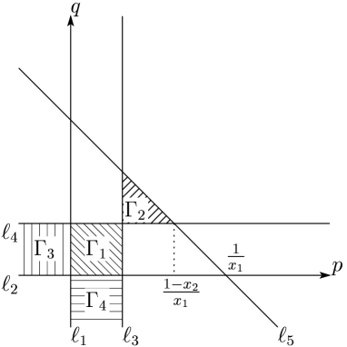
Figure 3. Images of $\Gamma_{i}$ in $\mathbb{P}^{2}$

Then $(1-\rho)\Gamma_{1},\dots,(1-\rho)\Gamma_{4}$ define elements in the relative homology $H_{2}(X,E_{1}\cup E_{2})_{\rho}.$ A holomorphic two form $\Omega_{X}$ on $X-D$ given by

$$\Omega_{X}= zdp\wedge dq\ \big{(}=p^{-\frac{2}{3}}q^{-\frac{2}{3}}(1-p)^{-\frac{2}{3}}(1-q)^{-\frac{2}{3}}(1-x_{1}p-x_{2}q)^{-\frac{2}{3}}dp\wedge dq\big{)}$$

becomes a global two form on $\widetilde{X}$, which is also denoted by $\Omega_{X}$. Since the restriction of $\Omega_{X}$ to $E_{1}\cup E_{2}$ is zero, it defines an element of the de Rham cohomology $H^{2}_{dR,c}(\widetilde{X}-E_{1}\cup E_{2})$ with compact support. The natural pairing

$$\langle\ ,\ \rangle:H_{2}(X,E_{1}\cup E_{2})_{\rho}\otimes H^{2}_{dR,c}(X-E_{1}\cup E_{2})_{\rho}\to\mathbb{C},$$

is defined by period integrals. We define functions $\varphi_{i}$ on $M$ by

(5.2) $$\varphi_{i}=\langle\Gamma_{i},\Omega_{X}\rangle=\int_{\Gamma_{i}}\Omega_{X},\quad(i=1,2,3,4).$$

Then we have a map

$$M\ni\vec{\ell}\mapsto(\varphi_{1},\dots,\varphi_{4})\in\mathbb{C}^{4}.$$

This map is continued analytically to a multivalued holomorphic map from $\mathcal{M}$ to $\mathbb{C}^{4}$.

Remark 5.1.

The integral $\varphi_{i}$ ($i=1,2,3,4$) satisfies Appell’s hypergeometric system $F_{2}$ of differential equations with parameters $(a,b_{1},b_{2},c_{1},c_{2})=(2/3,1/3,1/3,2/3,2/3)$.

5.2. Comparison of Period integrals

In this subsection, we compute period integrals using the isomorphisms in Proposition 4.5. Let $(x_{1},x_{2})$ be an element in $M$ defined in (5.1) and set

$$t=\dfrac{1-x_{1}-x_{2}}{(1-x_{1})(1-x_{2})}.$$

Then we have $0<t<1$ since $0<x_{1},x_{2},x_{1}+x_{2}<1$. Let $\lambda:E^{0}\times C^{0}\to{X^{\prime}}^{0}$ be a morphism defined in Proposition 2.4.

Proposition 5.2.

1. The pull back of the differential form $\Omega_{X}$ under the covering map $\lambda$ in (2.7) is equal to

   $$\lambda^{*}\Omega_{X}= (1-x_{1})^{-\frac{1}{3}}(1-x_{2})^{-\frac{1}{3}}w^{\prime}dr\wedge\psi_{1}$$

   $$= (1-x_{1})^{-\frac{1}{3}}(1-x_{2})^{-\frac{1}{3}}r^{-\frac{2}{3}}(1-r)^{-\frac{2}{3}}dr$$

   $$\wedge u^{-\frac{2}{3}}(1-u)^{-\frac{1}{3}}(1-tu)^{-\frac{1}{3}}du.$$

2. Via the isomorphism $\lambda$ in (2.6), The chains $\Gamma_{1},\Gamma_{2},\Gamma_{3}$ correspond to

   $$\Gamma_{1}^{\prime}= \{(ww^{\prime},r,u)\in(E_{\omega}\times C)/\langle\hat{\rho}\rangle\mid 0<r<1,-\infty<u<0,ww^{\prime}\in\mathbb{e}(\dfrac{1}{2})\},$$

   $$\Gamma_{2}^{\prime}= \{(ww^{\prime},r,u)\in(E_{\omega}\times C)/\langle\hat{\rho}\rangle\mid 1<r<\infty,\dfrac{1}{t}<u<\infty,ww^{\prime}\in\mathbb{e}(\dfrac{1}{6})\},$$

   $$\Gamma_{3}^{\prime}= \{(ww^{\prime},r,u)\in(E_{\omega}\times C)/\langle\hat{\rho}\rangle\mid 0<r<1,0<u<1-x_{1},ww^{\prime}\in\mathbb{e}(\dfrac{1}{3})\}.$$

We define $1$-chains $\gamma_{i}$ on $C$ by

$$\gamma_{1} =\{(w,u)\in C\mid u\in(-\infty,0),w\in\mathbb{e}(\dfrac{1}{2})\},$$

$$\gamma_{2} =\{(w,u)\in C\mid u\in(\dfrac{1}{t},\infty),w\in\mathbb{e}(\dfrac{1}{6})\},$$

$$\gamma_{3} =\{(w,u)\in C\mid u\in(0,1-x_{1}),w\in\mathbb{e}(\dfrac{1}{3})\}.$$

Then by the covering $\lambda:E\times C\to(E\otimes C)/\langle\hat{\rho}\rangle$, we have

(5.3) $$\Gamma_{i}^{\prime}=\lambda(\delta_{E}\otimes\gamma_{i})\quad(i=1,2,3),$$

where $\delta_{E}$ is defined in §3.1. Using the above relation, we have the following theorem.

Theorem 5.3.

The period integrals $\varphi_{i}$ $(i=1,2,3)$ are expressed as

$$\varphi_{i}(x_{1},x_{2})=(1-x_{1})^{-\frac{1}{3}}(1-x_{2})^{-\frac{1}{3}}B(\dfrac{1}{3},\dfrac{1}{3})\ \varphi^{\prime}_{i}(t)$$

for $i=1,2,3$, where $\varphi^{\prime}_{i}=\varphi^{\prime}_{i}(t)$ is

$$\varphi_{i}^{\prime}(t)=\int_{\gamma_{i}}u^{-\frac{2}{3}}(1-u)^{-\frac{1}{3}}(1-tu)^{-\frac{1}{3}}du.$$

The computation of the integral $\varphi_{4}(x_{1},x_{2})$ is reduced to that of $\varphi_{3}$ by exchanging the parameters $x_{1}\leftrightarrow x_{2}$, and the variables $p\leftrightarrow q$. We have

$$\varphi_{4}= B(\dfrac{1}{3},\dfrac{1}{3})(1-x_{1})^{-\frac{1}{3}}(1-x_{2})^{-\frac{1}{3}}\varphi_{4}^{\prime},$$

where

$$\varphi_{4}^{\prime} =\int_{\gamma_{4}}u^{-\frac{2}{3}}(1-u)^{-\frac{1}{3}}(1-tu)^{-\frac{1}{3}}du,$$

$$\gamma_{4} =\{(w,u)\in C\mid u\in(0,{1-x_{2}}),w\in\mathbb{e}(\dfrac{1}{3})\}.$$

5.3. Relations between cycles $\{\gamma_{i}\}$ and $\{\beta_{i}\}$ in $C$

We give relations between the bases $\{\gamma_{i}\}$ and $\{\beta_{i}\}$ of $H_{1}(C,\Sigma_{1}\cup\Sigma_{2})_{\rho}$. The action on $H_{1}(C,\Sigma_{1}\cup\Sigma_{2})_{\rho}$ induced by $\rho$ is also denoted as $\rho$. We define points $P_{0},P_{1},P_{t}$ and $P_{\infty}$ in $(u,w)\in C$ by

(5.4) $$P_{0}=(0,0),\quad P_{1}=(1,0),\quad P_{t}=(1/t,\infty),\quad P_{\infty}=(\infty,\infty).$$

Paths connecting $P_{0}$ with $P_{1},P_{t}$ and $P_{\infty}$ in the first sheet are denoted by $l_{1}$, $l_{t}$ and $l_{\infty}$, respectively. Then we have

(5.5) $$(1-\rho^{2})l_{1}=\beta_{1},\quad(1-\rho)l_{t}=\beta_{2},\quad(1-\rho)l_{\infty}=-\rho^{2}\beta_{1}+\beta_{2}.$$

Recall that $l_{1-x_{1}}$ and $l_{1-x_{2}}$ are paths in the first sheet from $P_{0}$ to the point with $u=1-x_{1}$ and that with $u=1-x_{2}$, respectively. The paths $l_{1-x_{1}}$ and $l_{1-x_{1}}$ and cycles $\beta_{1},\beta_{2},\beta_{4}$ satisfy the relations in (3.10).

Proposition 5.4.

In $H_{1}(C,\Sigma_{1}\cup\Sigma_{2})_{\rho}$, we have the following identities:

(5.6) $$\beta_{1} =\rho(1-\rho^{2})\gamma_{2},\quad\beta_{2}=(1-\rho^{2})\gamma_{1}+(1-\rho^{2})\gamma_{2},$$

$$\beta_{3} =(1-\rho)\gamma_{3},\quad\beta_{4}=(1-\rho^{2})\gamma_{4}-\rho^{2}(1-\rho^{2})\gamma_{2},$$

where $\gamma_{i}$ is defined in §5.2.

Proof.

The above identities follow from (3.6) and the identities

$$(1-\rho)\gamma_{1}=-(1-\rho)\rho l_{\infty},\quad(1-\rho)\gamma_{2}=(1-\rho)\rho(l_{\infty}-l_{t}),$$

$$(1-\rho)\gamma_{3}=(1-\rho)\rho l_{1-x_{1}},\quad(1-\rho)\gamma_{4}=(1-\rho)\rho l_{1-x_{2}}$$

in $H_{1}(C,\Sigma_{1}\cup\Sigma_{2})$. ∎

Proposition 5.5.

We set

$$B_{i}^{*}=\lambda(\delta_{E}\otimes\beta_{i})\quad(i=1,2,3).$$

Then $H_{2}(\widetilde{X},E_{2})_{\rho}$ is freely generated by $B_{1}^{*},B_{2}^{*}$ and $B_{3}^{*}$. We have the following relations between $B_{1}^{*},B_{2}^{*},B_{3}^{*}$ and $\Gamma_{1},\Gamma_{2},\Gamma_{3}$:

$$B_{1}^{*} =\rho(1-\rho^{2})\Gamma_{2},\ B_{2}^{*}=(1-\rho^{2})\Gamma_{1}+(1-\rho^{2})\Gamma_{2},\ B_{3}^{*}=(1-\rho)\Gamma_{3}.$$

As a consequence, $H_{2}(\widetilde{X},E_{2})_{\rho}$ is freely generated by $(1-\rho)\Gamma_{1},(1-\rho)\Gamma_{2}$ and $(1-\rho)\Gamma_{3}$.

Proof.

The first statement of the proposition is a consequence of Proposition 3.1, 4.5. By the equality (5.3), we have

$$\Gamma_{i}=\lambda(\delta_{E}\otimes\gamma_{i})\quad(i=1,2,3),$$

and the relations follow from (5.6). ∎

6. Period map for marked triple coverings of $\mathbb{P}^{2}$

In this section, we define a marking on a special configuration of $6$ lines in $\mathbb{P}^{2}$, and its moduli space $\mathcal{M}_{mk}$. We define the period map $\mathcal{M}_{mk}\to\mathbb{B}\times\mathbb{C}^{2}$ from the moduli space of marked configuration to a period domain (for the definition of $\mathbb{B}$, see (3.9)).

Let $\vec{\ell}=(x_{1},x_{2})$ be an element in $\mathcal{M}$. Recall that the triple covering $X=X_{\vec{\ell}}$ of $\mathbb{P}^{2}$ and the triple covering $C=C_{\vec{\ell}}$ of $\mathbb{P}^{1}$ are defined by the equations (2.1) and (2.2). Let $\Sigma_{i}$ be the subsets of $C$ defined in (3.5).

6.1. Level structures of monodromy curves and K3 surfaces

Let $(x_{1},x_{2})$ be an element in $\mathcal{M}$ (not necessarily contained in the domain $M$). We define mod $(1-\rho)$-markings of $H_{1}(C)$ and $H_{2}(\widetilde{X})_{\rho}$.

We begin with the mod $(1-\rho)$-marking of $H_{1}(C)$. We choose a path $l_{1}$ (resp. $l_{t},l_{1-x_{1}}$) in $C$ starting from the branching point $u=0$ and ending with $u=1$ (resp. $u=\dfrac{1}{t},1-x_{1}$). Since $(1-\rho)l_{1}$ (resp. $(1-\rho)l_{t},(1-\rho)l_{1-x_{1}}$) is an element in $H_{1}(C,\Sigma_{1})$, $l_{1}$ (resp. $l_{t},l_{1-x_{1}}$) is an element in $\dfrac{1}{1-\rho}H_{1}(C,\Sigma_{1})$ and defines a class $\overline{l_{1}}$ (resp. $\overline{l_{t}},\overline{l_{1-x_{1}}}$) in $\big{(}\dfrac{1}{1-\rho}H_{1}(C,\Sigma_{1})\big{)}/H_{1}(C,\Sigma_{1})$. We define $\mathbb{F}_{3}$-vector spaces $Z_{\mathbb{F}_{3}}$ and $H_{\mathbb{F}_{3}}$ by

$$Z_{\mathbb{F}_{3}} =\ker([P_{0}]\mathbb{F}_{3}\oplus[P_{1}]\mathbb{F}_{3}\oplus[P_{t}]\mathbb{F}_{3}\oplus[P_{\infty}]\mathbb{F}_{3}\to\mathbb{F}_{3})$$

$$a_{0}[P_{0}]+a_{1}[P_{1}]+a_{t}[P_{t}]+a_{\infty}[P_{\infty}]\mapsto a_{0}+a_{1}+a_{t}+a_{\infty},$$

$$H_{\mathbb{F}_{3}} =Z_{\mathbb{F}_{3}}/([P_{0}]-[P_{1}]-[P_{t}]+[P_{\infty}]).$$

It is easy to show the following lemma.

Lemma 6.1.

1. The classes $\overline{l_{1}},\overline{l_{t}}$ and $\overline{l_{1-x_{1}}}$ depend only on the end points $l_{1},l_{t}$ and $l_{1-x_{1}}$.

2. The $\mathbb{F}_{3}$-linear map $\mathcal{L}:\dfrac{1}{1-\rho}H_{1}(C)/H_{1}(C)\to H_{\mathbb{F}_{3}}$ defined by

   $$\mathcal{L}(\overline{l_{1}})=[P_{1}]-[P_{0}],\quad\mathcal{L}(\overline{l_{t}})=[P_{t}]-[P_{0}]$$

   is an isomorphism independent of the choice of $l_{1}$ and $l_{t}$.

We define the following classes in $\big{(}\dfrac{1}{1-\rho}H_{1}(C,\Sigma_{1})\big{)}/H_{1}(C,\Sigma_{1})$:

$$\big{[}\dfrac{1}{1-\rho}\beta_{1}\big{]}=-\overline{l_{1}},\quad\big{[}\dfrac{1}{1-\rho}\beta_{2}\big{]}=\overline{l_{t}},\quad\big{[}\dfrac{1}{1-\rho}\beta_{3}\big{]}=\overline{l_{1-x_{1}}}.$$

If $(x_{1},x_{2})$ belongs to $M$, then they coincide with the image of $\big{[}\dfrac{1}{1-\rho}\beta_{1}\big{]}$, $\big{[}\dfrac{1}{1-\rho}\beta_{2}\big{]}$ and $\big{[}\dfrac{1}{1-\rho}\beta_{3}\big{]}$ defined in §3.1 by the relations (5.5) and (3.6). Using symplectic basis $\{\alpha_{1},\alpha_{2},\beta_{1},\beta_{2}\}$ the elements $\overline{l_{i}}$ $(i=0,1,t,\infty)$ are written as

$$l_{i}\equiv\frac{1}{3}(-p_{i}U,p_{i})\begin{pmatrix}\alpha\\ \beta\end{pmatrix},\quad\alpha=\begin{pmatrix}\alpha_{1}\\ \alpha_{2}\end{pmatrix},\beta=\begin{pmatrix}\beta_{1}\\ \beta_{2}\end{pmatrix},\quad(i=0,1,t,\infty)$$

modulo $H_{1}(C)$, where

(6.1) $$p_{0}=(0,0),\quad p_{1}=(1,0),\quad p_{t}=(0,2),\quad p_{\infty}=(1,2).$$

Next we define the mod $(1-\rho)$ marking of $\widetilde{X}$ using the marking of $C$. By choosing a branch of $(1-x_{1})^{\frac{1}{3}}(1-x_{2})^{\frac{1}{3}}$, we obtain a rational map

$$\lambda:E\times C\dasharrow\widetilde{X}$$

by a morphism given in (2.6). By Proposition 4.5, the rational map $\lambda$ induces an isomorphism

$$\bigg{(}\dfrac{1}{1-\rho}H_{1}(E)\otimes_{\mathbb{Z}[\rho]}H_{1}(C,\Sigma_{1})\bigg{)}\bigg{/}\bigg{(}H_{1}(E)\otimes_{\mathbb{Z}[\rho]}H_{1}(C,\Sigma_{1})\bigg{)}$$

$$\xrightarrow[\simeq]{\lambda_{*}}\bigg{(}H_{2}(\widetilde{X},E_{2})_{\rho}\bigg{)}\bigg{/}\bigg{(}(1-\rho)H_{2}(\widetilde{X},E_{2})_{\rho}\bigg{)}.$$

The image of

$$\Delta_{E}\otimes\big{(}\dfrac{1}{1-\rho}\beta_{i}\big{)}=\delta_{E}\otimes\beta_{i}$$

under the map $\lambda_{*}$ is denoted by $\overline{B_{i}}$. One can show the following lemma easily.

Lemma 6.2.

The elements $\overline{B_{1}},\overline{B_{2}}$ and $\overline{B_{3}}$ in $\bigg{(}H_{2}(\widetilde{X},E_{2})_{\rho}\bigg{)}\bigg{/}\bigg{(}(1-\rho)H_{2}(\widetilde{X},E_{2})_{\rho}\bigg{)}$ do not depend on the choice of $(1-x_{1})^{\frac{1}{3}}(1-x_{2})^{\frac{1}{3}}$. The element $\overline{B_{i}}$ in $\bigg{(}H_{2}(\widetilde{X},E_{2})_{\rho}\bigg{)}\bigg{/}\bigg{(}(1-\rho)H_{2}(\widetilde{X},E_{2})_{\rho}\bigg{)}$ defined as above is denoted by $\overline{B_{i}}(X)$.

6.2. Moduli space $\mathcal{M}_{mk}$ of marked triple coverings of $\mathbb{P}^{2}$

6.2.1. The standard modules and bilinear forms

We set

$$W_{(-2)}=\langle B_{1},B_{2}\rangle_{\mathbb{Z}[\rho]}\subset W_{(-1)}=\langle B_{1},B_{2},B_{3}\rangle_{\mathbb{Z}[\rho]}.$$

Here $B_{1},B_{2},B_{3}$ form a formal free basis over $\mathbb{Z}[\rho]$. We use an identification $W_{(-1)}\simeq\mathbb{Z}[\rho]^{3}$ by writing an element $v$ in $W_{(-1)}$ by

(6.2) $$v=(c_{1},c_{2},c_{3})\begin{pmatrix}B_{1}\\ B_{2}\\ B_{3}\end{pmatrix},\quad c_{1},c_{2},c_{3}\in\mathbb{Z}[\rho].$$

Similarly, the submodule $W_{(-2)}$ is identified with $\{(c_{1},c_{2})\in\mathbb{Z}[\rho]^{2}\}$.

We define a $\mathbb{Z}[\rho]$-valued hermitian form $h(\ ,\ )$ and a $\mathbb{Z}$-valued symmetric bilinear form $\langle\ ,\ \rangle$ on $W_{(-2)}$ by

(6.3) $$h(x,y)=xU^{t}\overline{y},\quad\langle x,y\rangle=\dfrac{2}{3}\operatorname{Re}(h(x,y)),$$

where $U$ is given in (3.2).

6.2.2. Moduli space of marked of configurations

Definition 6.3 (Marked configuration).

We define a marked configuration by a pair $((x_{1},x_{2}),\mu)$ consisting of

1. a point $(x_{1},x_{2})$ in $\mathcal{M}$,

2. an isomorphism (marking) $\mu:W_{(-1)}\to H_{2}(\widetilde{X},E_{2})_{\rho}$ of $\mathbb{Z}[\rho]$-modules,

satisfying the following three conditions.

1. The image of $W_{(-2)}$ is identified with $H_{2}(\widetilde{X})_{\rho}$ under the map $\mu$. Under this isomorphism, the symmetric bilinear form on $W_{(-2)}$ and the intersection form on $H_{2}(\widetilde{X})_{\rho}$ are compatible.

2. Under the map

   $$W_{(-1)}/W_{(-2)}\to H_{2}(\widetilde{X},E_{2})_{\rho}/H_{2}(\widetilde{X})_{\rho}\simeq H_{1}(E_{2})$$

   induced by $\mu$, the element $B_{3}$ is sent to the classes of $\Delta_{E}$, where the second isomorphism is obtained by the exact sequence (4.4).

3. (Level structures) Let

   $$\overline{\mu}:W_{(-1)}/(1-\rho)W_{(-1)}\to H_{2}(\widetilde{X},E_{2})_{\rho}/(1-\rho)H_{2}(\widetilde{X},E_{2})_{\rho}$$

   be the map induced by the map $\mu$. Then the class of $B_{i}$ mod $(1-\rho)$ is mapped to the element $\overline{B_{i}}(X)$ defined in Lemma 6.2.

The set of marked configurations is denoted by $\mathcal{M}_{mk}$.

6.2.3. The case where $\vec{\ell}\in M$

A consequence of Proposition 4.2, we have the following proposition.

Proposition 6.4.

Let $\vec{\ell}=(x_{1},x_{2})\in M$. Using the element $\beta_{i}$ in $H_{1}(C)$ defined in §3.1, we define a $\mathbb{Z}[\rho]$-isomorphism $\mu:W_{(-1)}\to H_{2}(\widetilde{X},E_{2})_{\rho}$ by setting

$$\mu(B_{i})=\lambda(\delta_{E}\otimes\beta_{i}).$$

Then by the definition of $\overline{B_{i}}(X)$ in Lemma 6.2, Proposition 4.6, 5.5 and the relations (5.5) and (3.6), the pair $((x_{1},x_{2}),\mu)$ is a marked configuration.

Let $\mu:W_{(-2)}\to H_{2}(\widetilde{X})_{\rho}$ be a marking in Definition 6.3, and $\lambda:E\times C\dasharrow\widetilde{X}$ be a rational map in (2.6). Let $\beta_{1},\beta_{2}$ be elements in $H_{1}(C)$ such that

$$\mu(B_{i})=\lambda(\delta_{E}\otimes\beta_{i}).$$

Then we have the following proposition.

Proposition 6.5.

The set $\{\alpha_{1}=\rho(\beta_{2}),\alpha_{2}=\rho(\beta_{1}),\beta_{1},\beta_{2}\}$ forms a symplectic basis. Conversely, if $\{\alpha_{1},\alpha_{2},\beta_{1},\beta_{2}\}$ is a symplectic basis satisfying

(6.4) $$\alpha_{1}=\rho(\beta_{2}),\quad\alpha_{2}=\rho(\beta_{1}),$$

then the set $\{B_{1},B_{2}\}$ defined by $B_{i}=\mu^{-1}(\lambda(\delta_{E}\otimes\beta_{i}))$ ($i=1,2$) forms a basis of $H_{2}(\widetilde{X})_{\rho}$ and the intersection form is expressed as (6.3) with respect to this basis.

6.3. Period integrals of marked K3 surfaces

In this section, we define a period map from $\mathcal{M}_{mk}$ to $\mathbb{B}\times\mathbb{C}^{2}$ using the mixed Hodge structure of $H_{2}(X,E_{2})_{\rho}$. Let $\mu:W_{(-1)}\to H_{2}(\widetilde{X},E_{2})_{\rho}$ be a marking of $\widetilde{X}$.

We consider the following commutative diagrams for de Rham cohomologies:

$$\begin{matrix}0\to&H_{dR}^{1}(E_{2})(\chi)&\to&H_{dR,c}^{2}(\widetilde{X}-E_{2})(\chi)&\to&H_{dR}^{2}(\widetilde{X})(\chi)&\to 0\\ &&&\cup&&\cup\\ &&&F^{2}H_{dR,c}^{2}(\widetilde{X}-E_{2})(\chi)&\xrightarrow[\pi]{\simeq}&F^{2}H_{dR}^{2}(\widetilde{X})(\chi)\end{matrix}$$

$$\begin{matrix}0\to&H_{dR}^{1}(E_{2})(\overline{\chi})&\to&H_{dR,c}^{2}(\widetilde{X}-E_{2})(\overline{\chi})&\to&H_{dR}^{2}(\widetilde{X})(\overline{\chi})&\to 0\\ &&&\cup&&\cup\\ &&&F^{1}H_{dR,c}^{2}(\widetilde{X}-E_{2})(\overline{\chi})&\xrightarrow[\pi^{\prime}]{\simeq}&F^{1}H_{dR}^{2}(\widetilde{X})(\overline{\chi}).\end{matrix}$$

Proposition 6.6.

The spaces $F^{2}H_{dR}^{2}(\widetilde{X})(\chi)$ and $F^{1}H_{dR}^{2}(\widetilde{X})(\overline{\chi})$ are one dimensional over $\mathbb{C}$.

Proof.

Using the isomorphism (4.5), we have

$$F^{2}H_{dR}^{2}(\widetilde{X})(\chi)=\lambda^{*}(H^{10}(E)(\chi)\otimes H^{10}(C)(\chi)),$$

$$F^{1}H_{dR}^{2}(\widetilde{X})(\overline{\chi})=\lambda^{*}(H^{01}(E)(\overline{\chi})\otimes H^{10}(C)(\overline{\chi})).$$

Thus we have the proposition. ∎

By the above proposition, the spaces $F^{2}H_{dR}^{2}(\widetilde{X})(\chi)$ and $F^{1}H_{dR}^{2}(\widetilde{X})(\overline{\chi})$ can be regarded as one dimensional subspaces in

$$(W_{(-1)}\otimes\mathbb{C})(\chi)^{*}\xleftarrow{\mu}H_{dR,c}^{2}(\widetilde{X}-E_{2})(\chi)\text{ and }$$

$$(W_{(-1)}\otimes\mathbb{C})(\overline{\chi})^{*}\xleftarrow{\mu}H_{dR,c}^{2}(\widetilde{X}-E_{2})(\overline{\chi}).$$

This one dimensional vector spaces are expressed by a matrix $P((x_{1},x_{2}),\mu)$ in the following way. Let $\xi$ and $\xi^{\prime}$ be bases of $F^{2}H^{2}(\widetilde{X})(\chi)$ and $F^{1}H^{2}(\widetilde{X})(\overline{\chi})$. Via the isomorphism $\pi$ and $\pi^{\prime}$ in the above diagrams, $\xi$ and $\xi^{\prime}$ are regarded as elements in $H^{2}_{dR,c}(\widetilde{X}-E_{2})_{\rho}$. Using $\mu(B_{1}),\mu(B_{2}),\mu(B_{3})\in H_{2}(\widetilde{X},E_{2})_{\rho}$, we define the period matrix $P((x_{1},x_{2}),\mu)$ of a marked configuration $((x_{1},x_{2}),\mu)$ as follows

$$P((x_{1},x_{2}),\mu)=\begin{pmatrix}\langle\mu(B_{1}),\xi\rangle&\langle\mu(B_{1}),\xi^{\prime}\rangle\\ \langle\mu(B_{2}),\xi\rangle&\langle\mu(B_{2}),\xi^{\prime}\rangle\\ \langle\mu(B_{3}),\xi\rangle&\langle\mu(B_{3}),\xi^{\prime}\rangle\end{pmatrix}.$$

Here $\langle*,*\rangle$ is the pairing between the relative homology and the de Rham cohomology.

Proposition 6.7.

Let $((x_{1},x_{2}),\mu)$ be an element in $\mathcal{M}$ and $P((x_{1},x_{2}),\mu)$ be the period matrix of $((x_{1},x_{2}),\mu)$ defined as above. Then

(6.5) $$\dfrac{\langle\mu(B_{1}),\xi\rangle}{\langle\mu(B_{2}),\xi\rangle}=-\dfrac{\langle\mu(B_{1}),\xi^{\prime}\rangle}{\langle\mu(B_{2}),\xi^{\prime}\rangle},$$

and $\eta=\dfrac{\langle\mu(B_{1}),\xi\rangle}{\langle\mu(B_{2}),\xi\rangle}$ is an element of $\mathbb{B}$. The elements $\eta$ is independent of the choice of $\xi$ and $\xi^{\prime}$.

Proof.

The spaces $H_{dR}^{2}(\widetilde{X})(\chi)$ and $H_{dR}^{2}(\widetilde{X})(\overline{\chi})$ is identified with $\mathbb{C}^{2}$ via the following isomorphisms:

$$\varphi:H_{dR}^{2}(\widetilde{X})(\chi)\ni a\mapsto\varphi(a)=\begin{pmatrix}\langle\mu(B_{1}),a\rangle\\ \langle\mu(B_{2}),a\rangle\end{pmatrix}\in\mathbb{C}^{2},$$

$$\varphi^{\prime}:H_{dR}^{2}(\widetilde{X})(\overline{\chi})\ni a^{\prime}\mapsto\varphi(a)=\begin{pmatrix}\langle\mu(B_{1}),a^{\prime}\rangle\\ \langle\mu(B_{2}),a^{\prime}\rangle\end{pmatrix}\in\mathbb{C}^{2}.$$

Let $\pi_{\chi}$ (resp. $\pi_{\overline{\chi}}$) be the image of the projection to the $\chi$-part (resp. $\overline{\chi}$-part) according to the direct sum decomposition:

$$H_{2}(\widetilde{X})_{\rho}\otimes\mathbb{C}\simeq T_{X}^{*}\otimes\mathbb{C}\simeq H_{dR}^{2}(\widetilde{X})(\chi)\oplus H_{dR}^{2}(\widetilde{X})(\chi).$$

Then we have

$$\varphi(a_{1}\pi_{\chi}(B_{1})+a_{2}\pi_{\chi}(B_{2}))=\dfrac{1}{3}(a_{2},a_{1}),$$

$$\varphi^{\prime}(a_{1}\pi_{\overline{\chi}}(B_{1})+a_{2}\pi_{\overline{\chi}}(B_{2}))=\dfrac{1}{3}(a_{2},a_{1}).$$

Since the cup product is given by the formula (6.3), we have

$$a\cup a^{\prime}=3\cdot^{t}\varphi(a)U\varphi^{\prime}(a^{\prime})$$

for $a\in H_{dR}^{2}(\widetilde{X})(\chi),a^{\prime}\in H_{dR}^{2}(\widetilde{X})(\overline{\chi})$. Since $\xi$ and $\xi^{\prime}$ are contained in $F^{2}H^{2}_{dR}(X)(\chi)$ and $F^{1}H^{2}_{dR}(X)(\overline{\chi})$, we have $\xi\cup\xi^{\prime}=0$. Thus equality (6.5) follows.

The complex conjugate $H^{2}_{dR}(\widetilde{X})(\chi)\to H^{2}_{dR}(\widetilde{X})(\overline{\chi})$ with respect to $T_{X}^{*}$ is given by $\ {}^{t}(a_{1},a_{2})\to\ ^{t}(\overline{a_{1}},\overline{a_{2}})$ via the identification $\varphi$ and $\varphi^{\prime}$. By the positivity of the polarization, we have $\xi\cup\overline{\xi}>0$ for a nonzero element $\xi\in F^{2}H_{dR}^{2}(\widetilde{X})(\chi)$. Therefore $\operatorname{Re}(\eta)>0$. ∎

Definition 6.8.

We define the period domain $\mathcal{D}$ by

$$\mathcal{D}=\mathbb{B}\times\mathbb{C}^{2},$$

and $per:\mathcal{M}_{mk}\to\mathcal{D}$ by

$$per((x_{1},x_{2}),\mu)=(\eta,z)\in\mathcal{D}=\mathbb{B}\times\mathbb{C}^{2}.$$

Here, $\eta$ is defined in Proposition 6.7 and $z$ is defined by

$$z=\left(\frac{\langle\mu(B_{3}),\xi\rangle}{\langle\mu(B_{2}),\xi\rangle},\frac{\langle\mu(B_{3}),\xi^{\prime}\rangle}{\langle\mu(B_{2}),\xi^{\prime}\rangle}\right).$$

The vector $z$ is also independent of the choice of $\xi$ and $\xi^{\prime}$.

6.4. Transport of markings and a group action

6.4.1. Definition of $G(1-\rho)$ and its action on $W_{(-1)}$

We define subgroups $\Gamma$ and $\Gamma(1-\rho)$ of $GL(2,\mathbb{Z}[\rho])$ by

$$\Gamma =\{g\in GL(2,\mathbb{Z}[\rho])\mid gU\ ^{t}\overline{g}=U\},$$

$$\Gamma(1-\rho) =\{g\in\Gamma\mid g\equiv I_{2}\text{ mod }(1-\rho)\},$$

and a subgroup $G$ and $G(1-\rho)$ of $GL(3,\mathbb{Z}[\rho])$ by

$$G =\{\widetilde{g}=\begin{pmatrix}g&0\\ b&1\end{pmatrix}\in GL(3,\mathbb{Z}[\rho])\mid\ g\in\Gamma\},$$

$$G(1-\rho) =\{\widetilde{g}\in G\mid\ \widetilde{g}\equiv id\text{ mod }(1-\rho)\}.$$

The group $GL(3,\mathbb{Z}[\rho])$ acts on $W_{(-1)}$ from the right via the expression (6.2).

6.4.2. The action of $G(1-\rho)$ on $\mathcal{M}_{mk}$

Let $((x_{1},x_{2}),\mu)$ be a marked configuration and $\widetilde{g}$ an element in $G(1-\rho)$. By taking the composite $\mu\circ\widetilde{g}$ of $\widetilde{g}$ and the marking $\mu:W_{(-1)}\to H_{2}(X,E_{2})_{\rho}$, we get an action of $G(1-\rho)$ on $\mathcal{M}_{mk}$.

By the expression of the intersection form of the generic transcendental lattice of $\widetilde{X}$ obtained in Proposition 4.6, the action of $G(1-\rho)$ preserves the intersection form $\langle\ ,\ \rangle_{X}$ on $H_{2}(\widetilde{X})$. As a consequence, the group $G(1-\rho)$ acts on the moduli space $\mathcal{M}_{mk}$ of marked configurations.

Proposition 6.9.

The quotient of $\mathcal{M}_{mk}$ by $G(1-\rho)$ is isomorphic to $\mathcal{M}$.

Proof.

The natural map $\mathcal{M}_{mk}\to\mathcal{M}$ is surjective by definition of $\mathcal{M}_{mk}$. We show that the fiber $\mathcal{M}_{mk}\to\mathcal{M}$ is transitive under the action of $G(\rho-1)$. Let $(x_{1},x_{2})$ be an element in $\mathcal{M}$, and $((x_{1},x_{2}),\mu)$ and $((x_{1},x_{2}),\mu^{\prime})$ be two marked configurations. Let $\widetilde{g}={\mu^{\prime}}^{-1}\circ\mu$ be the composite map

$${\mu^{\prime}}^{-1}\circ\mu:W_{(-1)}\xrightarrow{\mu}H_{2}(\widetilde{X},E_{2})_{\rho}\xrightarrow{{\mu^{\prime}}^{-1}}W_{(-1)}.$$

Then $\widetilde{g}$ becomes an automorphism of $W_{(-1)}$ compatible with the $\rho$ action on $W_{(-1)}$. Since the submodule $W_{(-2)}$ is mapped isomorphically to the subspace $H_{2}(\widetilde{X})_{\rho}$ under the isomorphisms $\mu$ and $\mu^{\prime}$, the submodule $W_{(-2)}$ is stable under the isomorphism $\widetilde{g}$. Let $g$ be the restriction of $\widetilde{g}$ to the submodule $W_{(2)}$. Under the identifications $\mu$ and $\mu^{\prime}$ of $W_{(2)}$ with $H_{2}(\widetilde{X})_{\rho}$, intersection forms on $H_{2}(\widetilde{X})_{\rho}$ is transformed the inner product on $W_{(-2)}$. Since $g$ preserves the action of $\rho$, the hermitian form $h$ is preserved by $g$. Moreover by the condition for level structures for $\mu$ and $\mu^{\prime}$, $\overline{B}_{1},\overline{B}_{2}$ and $\overline{B}_{3}$ are mapped to $\overline{B}_{1}(X),\overline{B}_{2}(X)$ and $\overline{B}_{3}(X)$ by the isomorphisms

$$\overline{\mu},\overline{\mu^{\prime}}:W_{(-1)}/(1-\rho)W_{(-1)}\simeq H_{2}(\widetilde{X})_{\rho}/(1-\rho)H_{2}(\widetilde{X})_{\rho}.$$

Therefore we have $g\equiv I_{3}$ mod $(1-\rho)$. As a consequence, $g$ is an element in $G(1-\rho)$. ∎

6.4.3. The action of $G(1-\rho)$ on $\mathcal{D}$

The characters $\chi$ and $\overline{\chi}$ induce ring homomorphisms $\mathbb{Z}[\rho]\to\mathbb{C}$ and they induce group homomorphisms $GL(3,\mathbb{Z}[\rho])\to GL(3,\mathbb{C})$, which are also denoted by $\chi$ and $\overline{\chi}$.

Let $B_{1},B_{2},B_{3}$ be the $\mathbb{Z}[\rho]$-basis of $W_{(-1)}$ defined in §6.2.1. Using this basis, the group $G(1-\rho)$ acts on $W_{(-1)}$ via the identification given in (6.2). Thus an element $g$ in $G(1-\rho)$ acts on the set of the pairs of one dimensional vector spaces

$$\bigg{\{}(F^{2},F^{1})\ \bigg{|}\ \begin{matrix}F^{2}\subset(W_{(-1)}\otimes\mathbb{C})(\chi)^{*},\ F^{1}\subset(W_{(-1)}\otimes\mathbb{C})(\overline{\chi})^{*},\\ \dim(F^{2})=\dim(F^{1})=1\end{matrix}\bigg{\}}.$$

This action is expressed as

$$\chi(\widetilde{g})\times\overline{\chi}(\widetilde{g}):(\xi\mathbb{C},\overline{\xi}\mathbb{C})\mapsto(\chi(\widetilde{g})\xi\mathbb{C},\overline{\chi}(\widetilde{g})\overline{\xi}\mathbb{C}).$$

By transporting the structure, we have an action of $G(1-\rho)$ on $\mathcal{D}$, which is written as

$$(\eta,z)=(\eta,z_{1},z_{2})\mapsto(\frac{g_{11}\eta+g_{12}}{g_{21}\eta+g_{22}},\frac{z_{1}+w_{1}\eta+w_{2}}{g_{21}\eta+g_{22}},\frac{z_{2}-\overline{w_{1}}\eta+\overline{w_{2}}}{-\overline{g_{21}}\eta+\overline{g_{22}}}),$$

for

$$\widetilde{g}=\begin{pmatrix}g_{11}&g_{12}&0\\ g_{21}&g_{22}&0\\ w_{1}&w_{2}&1\end{pmatrix}\in G(1-\rho).$$

As a consequence, we have the following proposition.

Proposition 6.10.

The above action defines an associative action. Moreover the map $\mathcal{M}_{mk}\to\mathcal{D}$ is equivariant under the action of $G(1-\rho)$. By Proposition 6.9, we have a map

(6.6) $$\mathcal{M}\to\mathcal{D}/G(1-\rho).$$

6.5. Existence of an extra involution

Let $t$ be an element in $\mathbb{C}-\{0,1\}$, and $C$ be a curve defined by the equation (2.2).

Proposition 6.11.

1. There exists a symplectic basis $\{\alpha_{1},\alpha_{2},\beta_{1},\beta_{2}\}$ and an involution $\iota$ of $C$ satisfying the following properties.

   1. The relation (6.4) holds.

   2. The classes $\big{[}\dfrac{1}{1-\rho}\beta_{1}\big{]}$ and $\big{[}\dfrac{1}{1-\rho}\beta_{2}\big{]}$ in $\dfrac{1}{1-\rho}H_{1}(C)/H_{1}(C)$ are equal to $[P_{0}]-[P_{1}]$ and $[P_{t}]-[P_{0}]$ under the isomorphism $\mathcal{L}$ defined in Lemma 6.1.

   3. The following equalities hold:

      (6.7) $$\iota(\beta_{1})=\beta_{1},\quad\iota(\beta_{2})=-\beta_{2},\quad\iota\circ\rho=\rho^{-1}\circ\iota.$$

2. Let $\{\alpha_{1},\alpha_{2},\beta_{1},\beta_{2}\}$ be a symplectic basis satisfying the conditions (a), (b) of (1). Then there exists a unique involution $\iota$ of $C$ satisfying the equalities in (6.7).

We define an extra involution of $C$ for a general $t\in\mathbb{C}^{\{}0,1\}$.

Definition 6.12.

The involution $\iota$ satisfying these equalities is called the extra involution of $C$ with respect to the symplectic basis $\{\alpha_{1},\alpha_{2},\beta_{1},\beta_{2}\}$.

Proof.

(1) In §3.2, the existence of the above basis and the involution $\iota$ is proved in the case $(x_{1}^{0},x_{2}^{0})\in M$. For a general element $(x_{1}^{1},x_{2}^{1})$ in $\mathcal{M}$, we choose a path starting from $(x_{1}^{0},x_{2}^{0})$ and ending with a point $(x_{1}^{1},x_{2}^{1})\in M$. The values of $t$ at $(x_{1}^{0},x_{2}^{0})$ and $(x_{1}^{1},x_{2}^{1})$ are denoted by $t_{0}$ and $t_{1}$. Let $\beta_{1}^{0},\beta_{2}^{0}$ be topological cycles on $C_{t_{0}}$ defined in §3.1. Since the parameter $t$ varies continuously on $(x_{1},x_{2})$, $\beta_{1}^{0},\beta_{2}^{0}$ are deformed continuously and we get cycles $\beta_{1}^{1},\beta_{2}^{1}$ in $H_{1}(C_{t_{1}})$, which satisfy the properties (a), (b). The involution $\iota_{0}$ of the curve $C_{t_{0}}$ induces an involution $\overline{\iota_{0}}$ of $\mathbb{P}^{1}$ satisfying $\overline{\iota_{0}}(P_{0})=P_{1}$ and $\overline{\iota_{0}}(P_{t})=P_{\infty}$. We have a deformation $\overline{\iota_{t}}$ of the involution of $\mathbb{P}^{1}$ transposing $\{P_{0},P_{1}\}$ and $\{P_{t},P_{\infty}\}$ and get an involution $\overline{\iota_{1}}$ on $\mathbb{P}^{1}$ for $t=t_{1}$. We can lift the involution $\overline{\iota_{t}}$ of $\mathbb{P}^{1}$ to an involution $\iota_{t}$ of $C_{t}$ which is a deformation of $\iota_{0}$. Since $\iota_{t}$ is continuous on $t$, the equality (c) is preserved under this deformation.

(2) Let $\{\beta_{1},\beta_{2}\}$ be a $\mathbb{Z}[\rho]$-basis of $H_{1}(C)$ satisfying the condition (a), (b). We choose $\mathbb{Z}[\rho]$-basis $\{\beta^{\prime}_{1},\beta^{\prime}_{2}\}$ of $H_{1}(C)$, and an involution $\iota$ of $C$ satisfying the conditions (a), (b) and (c) of (1). Then we have

$$\begin{pmatrix}\beta_{1}^{\prime}\\ \beta_{2}^{\prime}\end{pmatrix}=g\begin{pmatrix}\beta_{1}\\ \beta_{2}\end{pmatrix},\quad g=\begin{pmatrix}a&b\\ c&d\end{pmatrix}\in\Gamma(1-\rho),$$

where $\Gamma(1-\rho)$ is defined in §6.4.1. We set $\displaystyle D=\begin{pmatrix}1&0\\ 0&-1\end{pmatrix}.$ Then we have

$$\begin{pmatrix}\iota(\beta_{1})\\ \iota(\beta_{2})\end{pmatrix} =\overline{g}\begin{pmatrix}\iota(\beta_{1}^{\prime})\\ \iota(\beta_{2}^{\prime})\end{pmatrix}=\overline{g}D\begin{pmatrix}\beta_{1}^{\prime}\\ \beta_{2}^{\prime}\end{pmatrix}=\overline{g}DU^{t}\overline{g}U\begin{pmatrix}\beta_{1}\\ \beta_{2}\end{pmatrix}$$

$$=\overline{ad-bc}\cdot D\begin{pmatrix}\beta_{1}\\ \beta_{2}\end{pmatrix}=\overline{\det(g)}\cdot D\begin{pmatrix}\beta_{1}\\ \beta_{2}\end{pmatrix}.$$

Since $g\in\Gamma(1-\rho)$, $\det(g)$ is a unit of $\mathbb{Z}[\rho]$ and congruent to $1$ mod $(1-\rho)$. Thus there exists $p\in\{0,1,2\}$ such that $\overline{\det(g)}=\rho^{p}$. By setting $\iota^{\prime}=\rho^{p}\iota\rho^{-p}$, we have $\iota^{\prime}\circ\rho=\rho^{-1}\circ\iota^{\prime}$ and

$$\begin{pmatrix}\iota^{\prime}(\beta_{1})\\ \iota^{\prime}(\beta_{2})\end{pmatrix}=\begin{pmatrix}\rho^{p}\iota\rho^{-p}(\beta_{1})\\ \rho^{p}\iota\rho^{-p}(\beta_{2})\end{pmatrix}=\begin{pmatrix}\rho^{-p}\iota(\beta_{1})\\ \rho^{-p}\iota(\beta_{2})\end{pmatrix}=\rho^{-p}\overline{\det(g)}D\begin{pmatrix}\iota(\beta_{1})\\ \iota(\beta_{2})\end{pmatrix}=D\begin{pmatrix}\iota(\beta_{1})\\ \iota(\beta_{2})\end{pmatrix}.$$

Therefore $\iota^{\prime}$ satisfies the condition (c). The uniqueness of $\iota$ can be proved similarly. ∎

Definition 6.13.

Let $\{\alpha_{1},\alpha_{2},\beta_{1},\beta_{2}\}$ be a symplectic basis satisfying the condition (a), (b) of Proposition 6.11 (1). The involution $\iota$ satisfying the condition (c) of Proposition 6.11(1) is called the extra involution associated to the basis $\{\alpha_{1},\alpha_{2},\beta_{1},\beta_{2}\}$. The element $\iota_{C*}\beta_{3}\in H_{1}(C,\Sigma_{2})$ is denoted by $\beta_{4}$.

Let $((x_{1},x_{2}),\mu)$ be an element in $\mathcal{M}_{mk}$. By choosing a branch of $(1-x_{1})^{\frac{1}{3}}(1-x_{2})^{\frac{1}{3}}$, we obtain a rational map $\lambda:E\times C\dasharrow\widetilde{X}$ as in (2.6) and elements $\beta_{1},\beta_{2},\beta_{3}$ in $H_{1}(C,\Sigma_{1})$ such that

$$\mu(B_{i})=\lambda_{*}(\delta_{E}\otimes\beta_{i}).$$

6.6. Coincidence of period maps for K3 surfaces and monodromy curves

6.6.1. The case $(x_{1},x_{2})\in\mathcal{M}$

We compute the period matrix $P((x_{1},x_{2}),\mu)$ for $(x_{1},x_{2})\in\mathcal{M}$ using the period integrals of the curve $C$. Let $\lambda:E\times C\dasharrow\widetilde{X}$ be a rational map in (2.6), and $\iota_{C}$ be the extra involution associated to $\mu$ and $\lambda$. Let $\psi_{1}$ be a non-zero element of $H^{0}(C,\it{\Omega}^{1}_{C})(\chi)$ and set

$$\psi_{2}=\iota_{C}^{*}(\psi_{1}).$$

Then we have $\psi_{2}\in H^{0}(C,\it{\Omega}_{C}^{1})(\overline{\chi})$. We choose elements $\Omega_{E}$ and $\Omega^{\prime}_{E}$ in $H^{1}(E)(\chi)$ and $H^{1}(E)(\overline{\chi})$ such that

$$\lambda^{*}\xi=\Omega_{E}\wedge\psi_{1},\quad\lambda^{*}\overline{\xi}=\Omega^{\prime}_{E}\wedge\psi_{2}.$$

We choose elements $\beta_{1},\beta_{2},\beta_{3}$ in $H_{1}(C,\Sigma_{1})$ such that

$$\mu(B_{i})=\lambda_{*}(\delta_{E}\otimes\beta_{i}).$$

By setting

$$c_{E}=\int_{\delta_{E}}\Omega_{E},\quad\overline{c_{E}}=\int_{\delta_{E}}\Omega_{E}^{\prime},$$

we have

$$\langle\mu(B_{i}),\xi\rangle=\langle\lambda_{*}(\delta_{E}\otimes\beta_{i}),\lambda^{*}(\xi)\rangle=\langle\delta_{E}\otimes\beta_{i},\Omega_{E}\wedge\psi_{1}\rangle=c_{E}\int_{\beta_{i}}\psi_{1},$$

$$\langle\mu(B_{i}),\overline{\xi}\rangle=\langle\delta_{E}\otimes\beta_{i},\Omega^{\prime}_{E}\wedge\psi_{2}\rangle=\overline{c_{E}}\int_{\beta_{i}}\psi_{2}=\overline{c_{E}}\int_{\beta_{i}}\iota_{C}^{*}\psi_{1}=\overline{c_{E}}\int_{\iota_{C*}\beta_{i}}\psi_{1}.$$

Since

$$\iota_{C*}\beta_{1}=\beta_{1},\quad\iota_{C*}\beta_{2}=-\beta_{2},\quad\iota_{C*}\beta_{3}=\beta_{4},$$

we have

(6.8) $$P((x_{1},x_{2}),\mu)= \begin{pmatrix}y_{1}&y_{1}\\ y_{2}&-y_{2}\\ y_{3}&y_{4}\end{pmatrix}\begin{pmatrix}c_{E}&0\\ 0&\overline{c_{E}}\\ \end{pmatrix},\quad y_{i}=\int_{\beta_{i}}\psi_{1}\quad(i=1,2,3,4).$$

Therefore by Definition 6.8, we have

(6.9) $$per((x_{1},x_{2}),\mu))=(\dfrac{y_{1}}{y_{2}},\dfrac{y_{3}}{y_{2}},\dfrac{y_{4}}{y_{2}}).$$

Definition 6.14.

We define a map

$$\jmath_{\mathcal{D}}:\mathcal{D}\ni(\eta,z)=(\eta,z_{1},z_{2})\mapsto(\tau(\eta),\zeta(z))\in\mathbb{H}_{2}\times\mathbb{C}^{2}$$

by

$$\tau=\frac{1}{2}\begin{pmatrix}\sqrt{-3}\eta^{-1}&-1\\ -1&\sqrt{-3}\eta\\ \end{pmatrix},$$

$$\zeta=\frac{1}{2}\left((\dfrac{z_{1}}{1-\omega}-\dfrac{z_{2}}{1-\omega^{2}})\eta^{-1},\dfrac{z_{1}}{1-\omega}+\dfrac{z_{2}}{1-\omega^{2}}\right).$$

By the equality (6.9), $\tau$ is the normalized period matrix of the curve $C$ for the symplectic base $\{\alpha_{1},\alpha_{2},\beta_{1},\beta_{2}\}$. We define the Jacobian $J(C)$ of the curve $C$ by

$$J(C)=\mathbb{C}^{2}/(\mathbb{Z}^{2}\tau\oplus\mathbb{Z}^{2}).$$

The class of $\zeta$ in the Jacobian $J(C)$ is equal to the image of Abel-Jacobi map for the integral on the path $l_{1-x_{1}}$ defined in §6.1.

6.6.2. The relation between $P((x_{1},x_{2}),\mu)$ and integrals $\varphi_{i}$ for $(x_{1},x_{2})\in M$

We give explicit computations of the period matrix in the case $(x_{1},x_{2})\in M$ given in (5.1). We choose the marking $\mu$ by setting $\mu(B_{i})=B_{i}^{*}$ for $i=1,2,3$, where $B_{i}^{*}$ are defined in Proposition 5.5. By this choice of $\mu$, the period matrix $P((x_{1},x_{2}),\mu)$ in (6.8) is computed from the integrals $\varphi_{1},\varphi_{2},\varphi_{3},\varphi_{4}$ in (5.2) as follows. We choose $\Omega_{E}$ and $\Omega^{\prime}_{E}$ so that $c_{E}=\overline{c_{E}}$. By the relation in Proposition 5.4, $y_{1},y_{2},y_{3},y_{4}$ in the left hand side of (6.8) are given by

$$c_{E}y_{1} =\omega(1-\omega^{2})\varphi_{2},\quad c_{E}y_{2}=(1-\omega^{2})\varphi_{1}+(1-\omega^{2})\varphi_{2},$$

$$c_{E}y_{3} =(1-\omega)\varphi_{3},\quad c_{E}y_{4}=(1-\omega^{2})\varphi_{4}-\omega^{2}(1-\omega^{2})\varphi_{2}.$$

6.7. Modular embedding

We set

$$Sp_{2}(\mathbf{Z}) =\Big{\{}g\in GL_{4}(\mathbf{Z})\Big{|}\;^{t}gJg=J=\begin{pmatrix}&-I\\ I&\end{pmatrix}\Big{\}},$$

$$\mathbb{H}_{2} =\{\tau\in GL_{2}(\mathbb{C})\mid\ ^{t}\tau=\tau,\quad\operatorname{Im}(\tau)>0\}.$$

We introduce a symplectic form on $\mathbb{Z}[\rho]\beta_{1}\oplus\mathbb{Z}[\rho]\beta_{2}$ by (3.3). Then $\alpha_{1}=\rho(\beta_{2}),\alpha_{2}=\rho(\beta_{1}),\beta_{1},\beta_{2}$ form a symplectic basis. Using this basis, we have inclusions $\jmath_{\Gamma}:\Gamma\to Sp_{2}(\mathbb{Z})$ and $\jmath_{G}:G(1-\rho)\to Sp_{2}(\mathbb{Z})\ltimes\mathbb{Z}^{4}$. More concretely, they are written as

$$\jmath_{H}:\mathbb{Z}[\rho]^{2}\ni(r_{1}+r_{2}\rho,s_{1}+s_{2}\rho)=(s_{2},r_{2},r_{1},s_{1})\in\mathbb{Z}^{4},$$

$$\jmath_{\Gamma}:\Gamma\ni g=g_{1}+g_{2}\rho\mapsto\begin{pmatrix}U(g_{1}-g_{2})U&-Ug_{2}\\ g_{2}U&g_{1}\end{pmatrix}\in Sp_{2}(\mathbf{Z}),$$

$$\jmath_{G}:G(1-\rho)\ni g=\begin{pmatrix}g&0\\ b&1\end{pmatrix}\ \mapsto\jmath_{\Gamma}(g)\ltimes\jmath_{H}(b)\in Sp_{2}(\mathbf{Z})\ltimes\mathbb{Z}^{4}.$$

By the construction, and the expression of $\zeta$ in (3.11), we have the following lemma.

Lemma 6.15.

The inclusion $\jmath_{\mathcal{D}}$ is compatible with the action of $G(1-\rho)$through $\jmath_{G}$ That is, we have

$$\jmath_{\mathcal{D}}(g\cdot x)=\jmath_{G}(g)\cdot\jmath_{\mathcal{D}}(x),\quad x\in\mathcal{D},\ g\in G(1-\rho).$$

7. Theta values and parameters of configurations

In this section, we show that the image of the period map $per:\mathcal{M}_{mk}\to\mathcal{D}$ coincides with the zero locus $V(\vartheta)$ of a theta function $\vartheta=\vartheta_{(-2,-1,1,2)/3}(\jmath_{\mathcal{D}}(\eta,z))$. Moreover, the map (6.6) induces an isomorphism $\overline{per}:\mathcal{M}\to V(\vartheta)/G(1-\rho)$. We construct the inverse of $\overline{per}$ using modular embedding defined in Definition 6.8 and theta functions (Theorem 7.6).

7.1. Theta function of the Jacobian $J(C)$ and inverse period map

The theta function $\vartheta_{a,b}$ of $(\tau,\zeta)\in\mathbf{H}_{2}\times\mathbf{C}^{2}$ with characteristics $(a,b)$ ($a,b\in\mathbb{Q}^{2}$) is defined by

$$\vartheta_{a,b}(\tau,\zeta)=\sum_{n\in\mathbf{Z}^{2}}\exp[\pi\sqrt{-1}\{(n+a)\tau\;^{t}(n+a)+2(n+a)\;^{t}(\zeta+b)\}].$$

In this section we study period map and its inverse using theta functions. The image of the map $\mathcal{M}_{mk}\to\mathcal{D}$ is characterized by the following theorem.

Definition 7.1.

We define an analytic space $V(\vartheta)$ of $\mathcal{D}$ by

$$V(\vartheta)=\{(\eta,z)\in\mathcal{D}\mid\vartheta_{(-2,-1,1,2)/3}(\jmath_{\mathcal{D}}(\eta,z))=0\}.$$

Theorem 7.2.

The image of $per:\mathcal{M}_{mk}\to\mathcal{D}$ coincides with $V(\vartheta)$.

We fix a real number $t$ satisfying $0<t<1$. Let $C=C_{t}$ be the curve defined in (2.2). We choose $x_{1}\in\mathbb{R}$ such that $0<x_{1}<1$. Then $x_{2}$ is determined by the equality (2.5). We use the symplectic basis in §3.1.

Let $p=(u,w)$ be the point on the second sheet in $C$ with $u=1-x_{1}$, and $\delta_{3}$ be a path from $P_{0}$ to $p$ on this sheet. Then $\zeta\in\mathbf{C}^{2}$ defined in (3.11) is a vector-valued function on $x_{1}$. This function is continued analytically to a holomorphic function $\zeta(\widetilde{p})$ on the universal covering $\widetilde{C}$ of $C$. Since $\zeta(\widetilde{p})$ is a multivalued function on $p$ in $C$, the function

$$\vartheta_{a,b}(p)=\vartheta_{a,b}(\tau(\eta),\zeta(p))$$

is a multivalued function on $p$. By the quasi periodicity of the theta function, a zero point of this function and its order are well defined on $J(C)$. Riemann’s theorem states that if $\vartheta_{a,b}(p)$ is not identically zero then it has two zero points with counting multiplicity.

Lemma 7.3.

For $m\in\mathbf{Z}^{2}$, the order of zero of

$$\vartheta_{[m]}(p)=\vartheta_{-mU/3,m/3}(p)$$

at $p=P_{i}$ $(i=0,1,t,\infty)$ is congruent to

$$(-1)^{r_{i}}(m+p_{i})U\;^{t}(m+p_{i})\bmod 3.$$

Here $P_{i}\in C$ and $p_{i}\in\mathbf{Z}^{2}$ are given in (5.4) and (6.1), respectively, and

$$r_{0}=1,\quad r_{1}=2,\quad r_{t}=2,\quad r_{\infty}=1.$$

Proof.

We use the following fundamental property: if a holomorphic function $f$ around $z=0$ satisfies

$$\lim_{z\to 0}\frac{f(\omega z)}{f(z)}=\omega^{k}\quad(k=0,1,2)$$

then the order of zero of $f(z)$ at $z=0$ is congruent to $k$ modulo $3$.

We consider the pull back $\rho^{*}(\vartheta_{[m]})(p)$ of $\vartheta_{[m]}(p)$ under the covering transformation $\rho$. One can choose a local parameter $v$ of $P_{0}$ (resp. $P_{1}$, $P_{t}$ and $P_{\infty}$) on a neighborhood $U_{0}$ (resp. $U_{1}$, $U_{t}$ and $U_{\infty}$) such that $\rho^{*}v=\omega v$ (resp. $\rho^{*}v=\omega^{2}v$, $\rho^{*}v=\omega^{2}v$ and $\rho^{*}v=\omega v$). For a point $p$ in the neighborhood $U_{i}$, we choose a path from $P_{i}$ to $p$ in $U_{i}$ and define a function

$$\vartheta_{[m]}^{i}(p)=\vartheta_{-(m+p_{i})U/3,(m+p_{i})/3}\left(\tau,\int_{P_{i}}^{p}\Psi\right),\quad\Psi=(\psi_{1},\psi_{2})(\tau_{B})^{-1}$$

on $U_{i}$, where $\psi_{1},\psi_{2}$ is defined in §3.1. Then we have $\vartheta_{[m]}(p)=h(p)\vartheta_{[m]}^{i}(p)$ for a non-zero holomorphic function $h(p)$.

We compute the limit $\lim\limits_{p\to P_{i}}\dfrac{\rho^{*}(\vartheta_{[m]}^{i}(p))}{\vartheta_{[m]}^{i}(p)}$ as follows. We have

$$\frac{\rho^{*}(\vartheta_{[m]}^{i}(p))}{\vartheta_{[m]}^{i}(p)} = \frac{\vartheta_{-(m+p_{i})U/3,(m+p_{i})/3}\left(\tau,\int_{P_{i}}^{p}\rho^{*}(\Psi)\right)}{\vartheta_{-(m+p_{i})U/3,(m+p_{i})/3}\left(\tau,\int_{P_{i}}^{p}\Psi\right)}$$

$$= \frac{\vartheta_{-(m+p_{i})U/3,(m+p_{i})/3}\left(\tau,\int_{P_{i}}^{p}\Psi(-U\tau-I_{2})^{-1}\right)}{\vartheta_{-(m+p_{i})U/3,(m+p_{i})/3}\left(\tau,\int_{P_{i}}^{p}\Psi\right)}$$

$$= \frac{\vartheta_{-(m+p_{i})U/3,(m+p_{i})/3}\left(\tau^{\#},\zeta^{\#}\right)}{\vartheta_{-(m+p_{i})U/3,(m+p_{i})/3}\left(\tau,\zeta\right)}.$$

Here we set $\tau^{\#}=\tau$, $\zeta=\int_{P_{i}}^{p}\Psi$ and $\zeta^{\#}=\zeta(-U\tau-I_{2})^{-1}$, and use

$$\rho^{*}(\Psi)=(\psi_{1},\psi_{2})W(\tau_{B})^{-1}=\Psi(U\tau)=\Psi(-U\tau-I_{2})^{-1},$$

where $\displaystyle W=\begin{pmatrix}\omega&0\\ 0&\omega^{2}\end{pmatrix}.$ Applying Corollary in p.85 and Corollary in p.176 of [I] to $\sigma=\rho^{-1}=\begin{pmatrix}O&U\\ -U&-I_{2}\end{pmatrix}\in Sp_{2}(\mathbf{Z})$, we can compute the limit of the last row as $p\to P_{i}$, and

$$\lim_{p\to P_{i}}\frac{\rho^{*}(\vartheta_{[m]}^{i}(p))}{\vartheta_{[m]}^{i}(p)}=\exp\left(\frac{2\pi\sqrt{-1}}{3}(-1)^{r_{i}}(m+p_{i})U\;^{t}(m+p_{i})\right).$$

The fundamental property yields this lemma. ∎

Lemma 7.3 yields a list of orders of zero of $\vartheta_{[m]}(p)$ at $P_{i}$ $(i=0,1,t,\infty)$ modulo $3$.

$[m]\diagdown p$	$P_{0}$	$P_{1}$	$P_{t}$	$P_{\infty}$
$[2,1]$	$2$	$0$	$0$	$0$
$[0,1]$	$0$	$2$	$0$	$0$
$[2,0]$	$0$	$0$	$2$	$0$
$[0,0]$	$0$	$0$	$0$	$2$
$[1,1]$	$1$	$1$	$0$	$0$
$[2,2]$	$1$	$0$	$1$	$0$
$[0,2]$	$0$	$1$	$0$	$1$
$[1,0]$	$0$	$0$	$1$	$1$
$[1,2]$	$2$	$2$	$2$	$2$

Table 1. List of orders of zero of $\vartheta_{[m]}(p)$

Proof of Theorem 7.2.

We fix an element $\eta\in\mathbb{B}$. By Table 1, $\vartheta_{[1,2]}(p)=\vartheta_{(-2,-1,1,2)/3}(\tau(\eta),\zeta(p))$ has zeros more then 2 (see [M]). Riemann’s theorem implies that this function of $p\in C$ is identically zero. Since the theta divisor is irreducible, the image of the period $[\zeta(p)]\in J(C)$ coincides with

$$\{[\zeta]\in J(C)\mid\vartheta_{(-2,-1,1,2)/3}(\tau(\eta),\zeta)=0\}.$$

∎

We have the following inverse period map for pairs $(C,p)$ of curve $C$ and a point $p$ on it.

Theorem 7.4.

Let $p=(u,w)$ be a point of $C$. The meromorphic function $u$ on $C$ is expressed as

(7.1) $$u=1-\frac{\vartheta_{[0,1]}^{3}(p)}{\vartheta_{[0,2]}^{3}(p)}=1-\frac{\vartheta_{(-1,0,0,1)/3}^{3}(\tau(\eta),\zeta(p))}{\vartheta_{(-2,0,0,2)/3}^{3}(\tau(\eta),\zeta(p))}.$$

In particular,

$$\frac{1}{t}=1-\frac{\vartheta_{(0,0,0,0)/3}^{3}(\tau(\eta))}{\vartheta_{(-1,0,0,1)/3}^{3}(\tau(\eta))}.$$

Remark 7.5.

The above formula for $t$ gives the inverse of the Schwartz map referred in Remark 3.4.

Proof.

(1) The divisor of the meromorphic function $1-u$ is $3P_{1}-3P_{\infty}$. By Table 1, $\vartheta_{[0,1]}(p)^{3}/\vartheta_{[0,2]}(p)^{3}$ has the same divisor. Thus their ratio is a constant. By putting $p=P_{0}$, we see that this constant is $1$. We obtain the expression of $1/t$ by substituting $p=P_{t}$ into (7.1) and using the formula

$$\vartheta_{a,b}(\tau,c\tau+d)=\exp[-\pi\sqrt{-1}(c\tau\;^{t}c+2c\;^{t}(b+d))]\vartheta_{a+c,b+d}(\tau,0)$$

for $a,b,c,d\in\mathbf{Q}^{2}$. ∎

7.2. Inverse period map for configuration space

Using Theorem 7.4, we give the inverse period map $V(\vartheta)/G(1-\rho)\to\mathcal{M}$ in terms of theta functions.

Theorem 7.6.

Let $((x_{1},x_{2}),\mu)$ be an element in $\mathcal{M}_{mk}$ and $(\eta,\zeta)=per((x_{1},x_{2}),\mu)\in\mathcal{D}$ be the image of $(x_{1},x_{2},\mu)$ under the period map $per$ defined in Definition 6.8. Let $\tau=\tau(\eta)$ be an element in $\mathbb{H}_{2}$ defined in §6.7.

Then the element $(x_{1},x_{2})\in\mathcal{M}$ is obtained by the following theta values:

$$x_{1} =\frac{\vartheta_{(-1,0,0,1)/3}^{3}(\tau,\zeta)}{\vartheta_{(-2,0,0,2)/3}^{3}(\tau,\zeta)},$$

$$x_{2} =\frac{\vartheta_{(-1,0,0,1)/3}^{3}(\tau,\iota^{*}(\zeta))}{\vartheta_{(-2,0,0,2)/3}^{3}(\tau,\iota^{*}(\zeta))},$$

where

$$\iota(\tau,\zeta)=(\tau,\iota^{*}(\zeta)),\quad\iota^{*}(\zeta)=\zeta\begin{pmatrix}1&0\\ 0&-1\end{pmatrix}+\left(0,\frac{\sqrt{3}\mathbf{i}}{3}\eta\right).$$

Proof.

By the condition of $x_{1},x_{2}$, we have $x_{1}x_{2}(1-x_{1})(1-x_{2})(1-x_{1}-x_{2})\neq 0$. We have a curve $C_{t}$ for $t=\dfrac{1-x_{1}-x_{2}}{(1-x_{1})(1-x_{2})}\in(0,1)$ and a point $p\in C_{t}$ whose $u$-coordinate is $1-x_{1}$. Apply to (7.1) for the point $p\in C_{t}$. Then we have

$$1-x_{1}=1-\frac{\vartheta_{(-1,0,0,1)/3}^{3}(\tau,\zeta)}{\vartheta_{(-2,0,0,2)/3}^{3}(\tau,\zeta)}.$$

This gives an expression of $x_{1}$ in terms of theta values at $(\tau,\zeta)$. To obtain the expression of $x_{2}$, we use theta values at $(\tau,\iota^{*}(\zeta))$ instead of $(\tau,\zeta)$ in the above expression. The vector $\iota^{*}(\zeta)$ is computed by $\dot{y}_{3}^{\prime}$ and $\dot{y}_{4}^{\prime}$ in stead of $y_{3}^{\prime}$ and $y_{4}^{\prime}$, where

$$\dot{y}_{3}^{\prime}=\int_{\widetilde{\Gamma}_{4}}\Omega_{X}\quad\dot{y}_{4}^{\prime}=\int_{\widetilde{\Gamma}_{3}}\Omega_{X}-\omega^{2}\int_{\widetilde{\Gamma}_{2}}\Omega_{X}.$$

Comparing with (5.6), (3.7) and (3.10), we have

$$\iota^{*}(\zeta) = \frac{1}{2}\left(\frac{\dot{y}_{3}^{\prime}+\dot{y}^{\prime}_{4}}{y_{1}},\frac{\dot{y}^{\prime}_{3}-\dot{y}_{4}^{\prime}}{y_{2}}\right)$$

$$= \frac{1}{2}\left(\frac{y_{3}^{\prime}+y^{\prime}_{4}}{y_{1}},\frac{y^{\prime}_{4}-y_{3}^{\prime}+(2\omega^{2}/(\omega-1))y_{1}}{y_{2}}\right)$$

$$= \frac{1}{2}\left(\frac{y_{3}^{\prime}+y^{\prime}_{4}}{y_{1}},-\frac{y^{\prime}_{3}-y_{4}^{\prime}}{y_{2}}\right)+\left(0,\frac{\sqrt{3}\mathbf{i}}{3}\eta\right).$$

∎

References

- [D] P. Deligne, Théorie de Hodge II, III, Publ. Math. IHES 40(1971), 5–57, 44(1974), 5–77.
- [I] J. Igusa, Theta Functions, Springer-Verlag, Berlin-Heidelberg-New York, 1972.
- [M] D. Mumford, Curves and their Jacobians, in The Red Book of Varieties and Schemes, Lecture Note in Math 1358, Springer.
- [MS] K. Matsumoto and H. Shiga, A variant of Jacobi type formula for Picard curves, J. Math. Soc. Japan., 62(2010), 305–319.
- [MSTY] K. Matsumoto, T. Sasaki, T. Terasoma and M. Yoshida, An example of Schwarz map of reducible Appell’s hypergeometric equation in two variables, to appear in J. Math. Soc. Japan.
- [S] T. Shioda, On the Mordell-Weil lattices, Comment. Math. Univ. Sancti-Pauli, 39 (1990), p. 211–240.