March 2017

Correlation functions and renormalization in a scalar field theory

on the fuzzy sphere

Kohta Hatakeyama and Asato Tsuchiya

Department of Physics, Shizuoka University
836 Ohya, Suruga-ku, Shizuoka 422-8529, Japan

We study renormalization in a scalar field theory on the fuzzy sphere. The theory is realized by a matrix model, where the matrix size plays the role of a UV cutoff. We define correlation functions by using the Berezin symbol identified with a field and calculate them nonperturbatively by Monte Carlo simulation. We find that the 2-point and 4-point functions are made independent of the matrix size by tuning a parameter and performing a wave function renormalization. The results strongly suggest that the theory is nonperturbatively renormalizable in the ordinary sense.

1 Introduction

It is conjectured that noncommutative geometry plays an essential role in the quantum theory of gravity. Indeed, it appears in various contexts of string theory (for a review, see [1].). For instance, field theories in noncommutative spaces are realized [2, 3] in the matrix models [4, 5, 6], which are proposals for nonperturbative formulation of string theory. Thus it is important to elucidate how field theories in noncommutative spaces differ from those in ordinary spaces. For this purpose, one needs to identify the behavior of basic quantities in field theories such as correlation functions.

One of the most important features of field theories in noncommutative spaces is that the product for fields is noncommutative and nonlocal. It yields IR divergences in perturbative expansion that originate from UV divergences. This phenomenon is called UV/IR mixing [7]and is known to be an obstacle to perturbative renormalization.

In this paper, we study multi-point correlation functions in a typical and simple example of a field theory in noncommutative spaces, a scalar field theory on the fuzzy sphere [8]. The theory is given by a matrix model, where the matrix size $N$ plays the role of a UV cutoff. There are several scaling limits where $N\rightarrow\infty$, corresponding to the continuum limits. Here, as a first approach to the above issue, it is reasonable to consider the so-called commutative limit where $N\rightarrow\infty$ with the radius of the sphere fixed, since the theory obtained in this limit is expected to be closest to the theory on the ordinary sphere. Indeed, as reviewed later, the former reduces to the latter in this limit at the classical (tree) level. However, it was shown in [9, 10] that the one-loop contribution to the self-energy in this limit is not IR divergent but differs by a finite and nonlocal term from that in the theory on the ordinary sphere. This difference is called the UV/IR anomaly and is a finite analog of the UV/IR mixing. It is important to see whether this sort of difference exists nonperturbatively or not, because it is possible that nonperturbative aspects of noncommutative field theory are relevant for quantum gravity.

Thus we calculate the correlation functions nonperturbatively by a performing Monte Carlo simulation (for a Monte Carlo study of the model, see [11, 12, 13, 14, 15]. For a related analytic study of the model, see [16, 17, 18, 19, 20, 21, 22, 23, 24].). Here, in particular, we focus on renormalization, one of the most basic properties of field theories. We will see whether the theory is renormalized in the ordinary manner; namely, whether the multi-point correlation functions become independent of the UV cutoff $N$ if some parameters are tuned and a wave function renormalization is performed. Such nonperturbative renormalization in a nonlocal field theory should be nontrivial. The authors of [25, 26] examined the dispersion relation and so on in scalar field theories on the noncommutative torus by calculating the 2-point correlation functions nonperturbatively by Monte Carlo simulation and concluded that the theories are nonperturbatively renormalizable in the double scaling limit where the continuum and thermodynamic limits are simultaneously taken at fixed noncommutative tensor. The theories obtained in the double scaling limit are obviously different from field theories in ordinary spaces. A similar analysis for gauge theories on the noncommutative torus was performed in [27, 28].

Here, we find that the 2-point and 4-point correlation functions are independent of $N$ if a parameter is tuned and a wave function renormalization is performed. These results strongly suggest that the theory is nonperturbatively renormalizable in the ordinary sense and enable us to conjecture that the theory is specified by a parameter. To support this conjecture, we examine the theory at a fixed $N$. This is the first Monte Carlo study of renormalization on the fuzzy sphere.

To define the correlation functions, we regard the Berezin symbol [29] of the matrix constructed from the Bloch coherent state [30] as a field. As far as we know, the coherent state is used for the first time in Monte Carlo study of noncommutative field theories. Thus another aim of this paper is to demonstrate that the method developed here is a powerful one for Monte Carlo study of noncommutative field theories. We expect the method to be applied not only to the other limits of the theory but also to other field theories in noncommutative spaces.

This paper is organized as follows. In section 2, we review a scalar field theory on the fuzzy sphere, which is realized by a matrix model. We compare it with a corresponding field theory on the sphere by identifying the Berezin symbol constructed from the matrix with the field. In section 3, we define the correlation functions that we calculate by Monte Carlo simulation, and show the results of the simulations. Section 4 is devoted to the conclusion and discussion. In appendix A, we review the Bloch coherent state, the Berezin symbol and the star product on the fuzzy sphere. In appendix B, we show the results for the 1-point functions.

2 Scalar field theory on the fuzzy sphere

Let us consider a scalar field theory on a sphere with the radius $R$:

$$S_{C}=\frac{R^{2}}{4\pi}\int d\Omega\left(-\frac{1}{2R^{2}}({\cal L}_{i}\phi)^{2}+\frac{\mu^{2}}{2}\phi^{2}+\frac{\lambda}{4}\phi^{4}\right)\ ,$$ (2.1)

where ${\cal L}_{i}$ $(i=1,2,3)$ are the orbital angular momentum operators and $d\Omega$ is the invariant measure on the sphere. We parametrize the sphere by the standard polar coordinates $(\theta,\varphi)$. Then ${\cal L}_{i}$ and $d\Omega$ take the following form:

$${\cal L}_{\pm} \equiv{\cal L}_{1}\pm i{\cal L}_{2}=e^{\pm i\varphi}\left(\pm\frac{\partial}{\partial\theta}+i\cot\theta\frac{\partial}{\partial\varphi}\right)\ ,$$

$${\cal L}_{3} =-i\frac{\partial}{\partial\varphi}\ ,$$ (2.2)

and $d\Omega=\sin\theta d\theta d\varphi$.

A noncommutative counterpart of (2.1) is given by a matrix model:

$$S=\frac{R^{2}}{2j+1}\mbox{Tr}\left(-\frac{1}{2R^{2}}[L_{i},\Phi]^{2}+\frac{\mu^{2}}{2}\Phi^{2}+\frac{\lambda}{4}\Phi^{4}\right)\ ,$$ (2.3)

where $j$ is a non-negative integer or half-integer, and $\Phi$ is a $(2j+1)\times(2j+1)$ Hermitian matrix. $L_{i}$ are the generators of the $SU(2)$ algebra with the spin $j$ representation, obeying the commutation relation $[L_{i},L_{j}]=i\epsilon_{ijk}L_{k}$. $j$ plays the role of a UV cutoff. We also denote the matrix size by $N$; namely, $N=2j+1$.

In this paper, we are concerned with the so-called commutative limit, where $N\rightarrow\infty$ with $R$ fixed. Hereafter, we put $R=1$ without loss of generality. We briefly review below that (2.3) reduces to (2.1) at the classical level in this limit while the former differs from the latter due to the UV/IR anomaly at the quantum level.

Here, in order to see the correspondence between the above two theories, we introduce the Bloch coherent state[30] and the Berezin symbol[29]. The Bloch coherent state denoted by $|\Omega\rangle$ ($\Omega=(\theta,\varphi)$) is localized around the point $(\theta,\varphi)$ on the sphere. The basic properties of the Bloch coherent state are reviewed in appendix A.

The Berezin symbol for an $N\times N$ matrix $A$ is defined by

$$f_{A}(\Omega)=\langle\Omega|A|\Omega\rangle\ .$$ (2.4)

By using (A.7), one can easily show that

$$f_{[L_{i},A]}(\Omega)={\cal L}_{i}f_{A}(\Omega)\ .$$ (2.5)

Also, (A.10) implies that

$$\frac{1}{2j+1}\mbox{Tr}(A)=\int\frac{d\Omega}{4\pi}f_{A}(\Omega)\ .$$ (2.6)

The star product for the Berezin symbols is defined by

$$f_{A}\star f_{B}(\Omega)=\langle\Omega|AB|\Omega\rangle\ ,$$ (2.7)

where $A$ and $B$ are $N\times N$ matrices. To express the star product in terms of the Berezin symbol, we use the stereographic projection given by

$$z=\tan\frac{\theta}{2}e^{i\varphi}$$ (2.8)

and denote the Bloch coherent state $|\Omega\rangle$ by $|z\rangle$ and the Berezin symbol $f_{A}(\Omega)$ by $f_{A}(z,\bar{z})$. Then, the star product is expressed as

$$f_{A}\star f_{B}(w,\bar{w})=\frac{2j+1}{4\pi}4\int\frac{d^{2}z}{(1+|z|^{2})^{2}}(e^{-w\frac{\partial}{\partial z}}e^{z\frac{\partial}{\partial w}}f_{A}(w,\bar{w}))(e^{-\bar{w}\frac{\partial}{\partial\bar{z}}}e^{\bar{z}\frac{\partial}{\partial\bar{w}}}f_{B}(w,\bar{w}))|\langle w|z\rangle|^{2}$$ (2.9)

as shown in appendix A. This shows that the star product is nonlocal and noncommutative. Furthermore, it is easy to show that in the $j\rightarrow\infty$ limit

$$\frac{2j+1}{4\pi}\frac{4}{(1+|z|^{2})^{2}}|\langle w|z\rangle|^{2}\rightarrow\delta^{2}(z-w)\ .$$ (2.10)

This implies that in the $j\rightarrow\infty$ limit the star product reduces to the ordinary product. Namely,

$$f_{A}\star f_{B}(w,\bar{w})\rightarrow f_{A}(w,\bar{w})f_{B}(w,\bar{w})$$ (2.11)

or

$$f_{A}\star f_{B}(\Omega)\rightarrow f_{A}(\Omega)f_{B}(\Omega)\ .$$ (2.12)

(2.5), (2.6) and (2.12) show that the theory (2.3) reduces to the one (2.1) in the commutative ($N\rightarrow\infty$) limit at the classical (tree) level if $f_{\Phi}(\Omega)$ is identified with $\phi(\Omega)$. However, as shown to the one-loop order in [9, 10], (2.3) differs from (2.1) by a finite and nonlocal term because the UV cutoff $N$ must be kept finite in calculating the radiative corrections. Namely, the quantization and the commutative limit are not commutative. This phenomenon is called the UV/IR anomaly.

3 Correlation functions

3.1 Definition of correlation functions

For later convenience, we introduce a shorthand notation for the Berezin symbol:

$$\varphi(\Omega)=f_{\Phi}(\Omega)=\langle\Omega|\Phi|\Omega\rangle\ .$$ (3.1)

In the theory (2.3), the $n$-point correlation function is defined by

$$\left\langle\varphi(\Omega_{1})\varphi(\Omega_{2})\cdots\varphi(\Omega_{n})\right\rangle=\frac{\int d\Phi\ \varphi(\Omega_{1})\varphi(\Omega_{2})\cdots\varphi(\Omega_{n})\ e^{-S}}{\int d\Phi\ e^{-S}}\ ,$$ (3.2)

where

$$d\Phi=\prod_{i=1}^{N}d\Phi_{ii}\prod_{1\leq j<k\leq N}d\mbox{Re}\Phi_{jk}d\mbox{Im}\Phi_{jk}\ .$$ (3.3)

The correlation function (3.2) is an analog of $\langle\phi(\Omega_{1})\phi(\Omega_{2})\cdots\phi(\Omega_{n})\rangle$ in the theory (2.1).

Suppose that the matrix $\Phi$ in (2.3) is renormalized as

$$\Phi=\sqrt{Z}\Phi_{r}\ ,$$ (3.4)

where $Z$ is a factor of the wave function renormalization, and $\Phi_{r}$ is the renormalized matrix. Correspondingly, the renormalized Berezin symbol $\varphi_{r}(\Omega)$ is defined by

$$\varphi(\Omega)=\sqrt{Z}\varphi_{r}(\Omega)\ ,$$ (3.5)

and the renormalized $n$-point correlation function $\left\langle\varphi_{r}(\Omega_{1})\varphi_{r}(\Omega_{2})\cdots\varphi_{r}(\Omega_{n})\right\rangle$ is defined by

$$\left\langle\varphi(\Omega_{1})\varphi(\Omega_{2})\cdots\varphi(\Omega_{n})\right\rangle=Z^{\frac{n}{2}}\left\langle\varphi_{r}(\Omega_{1})\varphi_{r}(\Omega_{2})\cdots\varphi_{r}(\Omega_{n})\right\rangle\ .$$ (3.6)

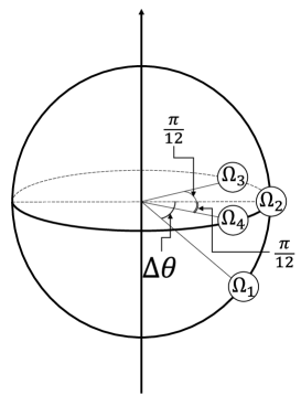
Figure 1: Four points on the sphere selected for the correlation functions.

In the following, we calculate the following correlation functions by Monte Carlo simulation:

$$\mbox{1-point function:}\;\left\langle\varphi(\Omega_{1})\right\rangle\ ,$$

$$\mbox{2-point function:}\;\left\langle\varphi(\Omega_{p})\varphi(\Omega_{q})\right\rangle\;(1\leq p<q\leq 4)\ ,$$

$$\mbox{4-point function:}\;\left\langle\varphi(\Omega_{1})\varphi(\Omega_{2})\varphi(\Omega_{3})\varphi(\Omega_{4})\right\rangle\ .$$ (3.7)

We show in appendix B that the 1-point functions vanish. Thus, the 2-point function is itself the connected one, while the connected 4-point function is defined by

$$\left\langle\varphi(\Omega_{1})\varphi(\Omega_{2})\varphi(\Omega_{3})\varphi(\Omega_{4})\right\rangle_{c}= \left\langle\varphi(\Omega_{1})\varphi(\Omega_{2})\varphi(\Omega_{3})\varphi(\Omega_{4})\right\rangle-\left\langle\varphi(\Omega_{1})\varphi(\Omega_{2})\right\rangle\left\langle\varphi(\Omega_{3})\varphi(\Omega_{4})\right\rangle$$

$$-\left\langle\varphi(\Omega_{1})\varphi(\Omega_{3})\right\rangle\left\langle\varphi(\Omega_{2})\varphi(\Omega_{4})\right\rangle-\left\langle\varphi(\Omega_{1})\varphi(\Omega_{4})\right\rangle\left\langle\varphi(\Omega_{2})\varphi(\Omega_{3})\right\rangle\ .$$ (3.8)

The renormalized correlation functions are defined as

$$\left\langle\varphi(\Omega_{1})\right\rangle =\sqrt{Z}\left\langle\varphi_{r}(\Omega_{1})\right\rangle\ ,$$ (3.9)

$$\left\langle\varphi(\Omega_{p})\varphi(\Omega_{q})\right\rangle =Z\left\langle\varphi_{r}(\Omega_{p})\varphi_{r}(\Omega_{q})\right\rangle\ ,$$ (3.10)

$$\left\langle\varphi(\Omega_{1})\varphi(\Omega_{2})\varphi(\Omega_{3})\varphi(\Omega_{4})\right\rangle_{c} =Z^{2}\left\langle\varphi_{r}(\Omega_{1})\varphi_{r}(\Omega_{2})\varphi_{r}(\Omega_{3})\varphi_{r}(\Omega_{4})\right\rangle_{c}\ .$$ (3.11)

We choose $\Omega_{p}=(\theta_{p},\varphi_{p})$ $(p=1,2,3,4)$ as follows (see Fig.1):

$$\Omega_{1} =\left(\frac{\pi}{2}+\Delta\theta,\ 0\right)\ ,$$

$$\Omega_{2} =\left(\frac{\pi}{2},\ 0\right)\ ,$$

$$\Omega_{3} =\left(\frac{\pi}{2},\ \frac{\pi}{12}\right)\ ,$$

$$\Omega_{4} =\left(\frac{\pi}{2},\ -\frac{\pi}{12}\right)\ ,$$ (3.12)

where $\Delta\theta$ is taken from $0.3$ to $1.5$ in steps of $0.1$.

3.2 Renormalization

We use the hybrid Monte Carlo method to calculate the correlation functions (3.7).

First, we simulate at $N=32$, $\mu^{2}=-11.5$ and $\lambda=1.0$. Then, keeping $\lambda=1.0$, we simulate at $N=24$ and various values of $\mu^{2}$. In Fig.2, we plot

$$\log\left\langle\varphi(\Omega_{1})\varphi(\Omega_{2})\right\rangle=\log Z+\log\left\langle\varphi_{r}(\Omega_{1})\varphi_{r}(\Omega_{2})\right\rangle$$ (3.13)

against $\Delta\theta$ at $N=32$ and $\mu^{2}=-11.5$ and at $N=24$ and typical values of $\mu^{2}$, $-7.97,-12.0,-6.0$. We see that the data for $N=24$ and $\mu^{2}=-7.97$ agree with those for $N=32$ and $\mu^{2}=-11.5$ if the former are simultaneously shifted in the vertical direction and that this is not the case for the data for $N=24$ and $\mu^{2}=-12.0,-6.0$. This implies that the renormalized 2-point function at $N=24$ and $\mu^{2}=-7.97$ agrees with that at $N=32$ and $\mu^{2}=-11.5$ and that we can determine

$$\alpha_{24\rightarrow 32}\equiv\log\left(\frac{Z(32)}{Z(24)}\right)\ .$$ (3.14)

Indeed, by using the least-squares method, we obtain $\alpha_{24\rightarrow 32}=0.2334$ with the error $\delta\alpha_{24\rightarrow 32}=0.0108$. In Fig.3, we plot $\left\langle\varphi(\Omega_{1})\varphi(\Omega_{2})\right\rangle$ at $N=32$ and $\mu^{2}=-11.5$ and $\zeta_{24\rightarrow 32}\left\langle\varphi(\Omega_{1})\varphi(\Omega_{2})\right\rangle$ at $N=24$ and $\mu^{2}=-7.97$ against $\Delta\theta$, where

$$\zeta_{24\rightarrow 32}=e^{\alpha_{24\rightarrow 32}}=\frac{Z(32)}{Z(24)}=1.263\ .$$ (3.15)

We indeed see a good agreement between the data for $N=24$ and thoes for $N=32$.

Furthermore, we can expect that the renormalized connected 4-point function at $N=24$ agrees with that at $N=32$. Indeed, in Fig.4, we plot $\left\langle\varphi(\Omega_{1})\varphi(\Omega_{2})\varphi(\Omega_{3})\varphi(\Omega_{4})\right\rangle_{c}$ at $N=32$ and $\mu^{2}=-11.5$ and $\zeta_{24\rightarrow 32}^{2}\left\langle\varphi(\Omega_{1})\varphi(\Omega_{2})\varphi(\Omega_{3})\varphi(\Omega_{4})\right\rangle_{c}$ at $N=24$ and $\mu^{2}=-7.97$ against $\Delta\theta$. We again see a good agreement between the data for $N=24$ and thoes for $N=32$, which implies that the renormalized connected 4-point function at $N=24$ agrees with that at $N=32$.

Similarly, we simulate at $N=40$ and various values of $\mu^{2}$, keeping $\lambda=1.0$. We perform the same analyses for $N=40$ and $N=32$ in Fig.5, Fig.6, and Fig.7 as for $N=24$ and $N=32$ in Fig.2, Fig.3, and Fig.4, respectively. In Fig.5, we show the results for $\log\left\langle\varphi(\Omega_{1})\varphi(\Omega_{2})\right\rangle$ at $N=40$ and typical values of $\mu^{2}$, $-14.08,-16.0,-12.0$. We find that $N=40$ and $\mu^{2}=-14.08$ corresponds to $N=32$ and $\mu^{2}=-11.5$. In Fig.6 and Fig.7, we confirm that the 2-point function and the connected 4-point function at $N=40$ and $\mu^{2}=-14.08$ with the wave function renormalization agree with those at $N=32$ and $\mu^{2}=-11.5$.

The values of $\alpha$ and $\zeta$ that we have determined are summarized in Table1. The above results strongly suggest that the renormalized correlation functions are independent of $N$ and that the theory (2.3) is nonperturbatively renormalizable in the ordinary sense.

$N^{\prime}\rightarrow N$	$\alpha_{N^{\prime}\rightarrow N}$	$\delta\alpha_{N^{\prime}\rightarrow N}$	$\zeta_{N^{\prime}\rightarrow N}$	$\zeta_{N^{\prime}\rightarrow N}^{2}$
$24\rightarrow 32$	$0.2334$	$0.0108$	$1.263$	$1.595$
$40\rightarrow 32$	$-0.1489$	$0.0101$	$0.8617$	$0.7425$

Table 1: $\alpha_{N^{\prime}\rightarrow N}$, $\delta\alpha_{N^{\prime}\rightarrow N}$, $\zeta_{N^{\prime}\rightarrow N}$ and $\zeta_{N^{\prime}\rightarrow N}^{2}$.

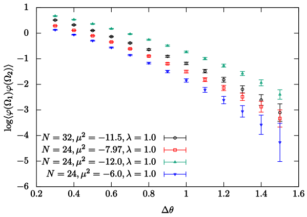
Figure 2: $\log\left\langle\varphi(\Omega_{1})\varphi(\Omega_{2})\right\rangle$ at $\lambda=1.0$ is plotted against $\Delta\theta$. The data for $N=32$ and $\mu^{2}=-11.5$ are represented by the circles, while the data for $N=24$ and $\mu^{2}=-7.97,-12.0,-6.0$ are represented by the squares, the triangles and the inverted triangles, respectively.

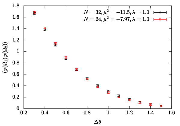
Figure 3: $\left\langle\varphi(\Omega_{1})\varphi(\Omega_{2})\right\rangle$ at $N=32$, $\mu^{2}=-11.5$ and $\lambda=1.0$ is plotted against $\Delta\theta$, where the data are represented by the circles. $\zeta_{24\rightarrow 32}\left\langle\varphi(\Omega_{1})\varphi(\Omega_{2})\right\rangle$ with $\zeta_{24\rightarrow 32}=1.263$ at $N=24$, $\mu^{2}=-7.97$ and $\lambda=1.0$ is also plotted against $\Delta\theta$, where the data are represented by the squares.

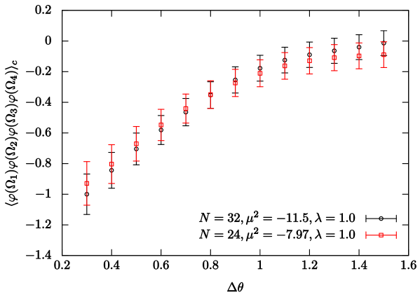
Figure 4: $\left\langle\varphi(\Omega_{1})\varphi(\Omega_{2})\varphi(\Omega_{3})\varphi(\Omega_{4})\right\rangle_{c}$ at $N=32$, $\mu^{2}=-11.5$ and $\lambda=1.0$ is plotted against $\Delta\theta$, where the data are represented by the circles. $\zeta_{24\rightarrow 32}^{2}\left\langle\varphi(\Omega_{1})\varphi(\Omega_{2})\varphi(\Omega_{3})\varphi(\Omega_{4})\right\rangle_{c}$ with $\zeta_{24\rightarrow 32}^{2}=1.595$ at $N=24$, $\mu^{2}=-7.97$ and $\lambda=1.0$ is also plotted against $\Delta\theta$, where the data are represented by the squares.

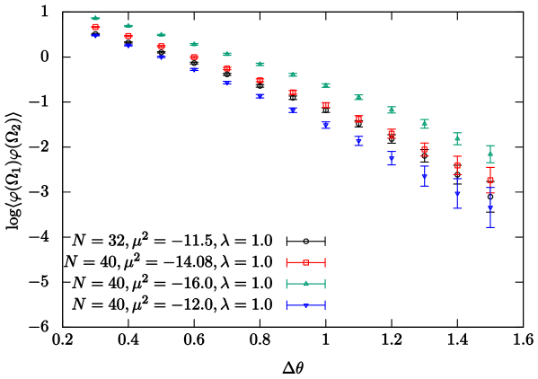
Figure 5: $\log\left\langle\varphi(\Omega_{1})\varphi(\Omega_{2})\right\rangle$ at $\lambda=1.0$ is plotted against $\Delta\theta$. The data for $N=32$ and $\mu^{2}=-11.5$ are represented by the circles, while the data for $N=40$ and $\mu^{2}=-14.08,-16.0,-12.0$ are represented by the squares, the triangles and the inverted triangles, respectively.

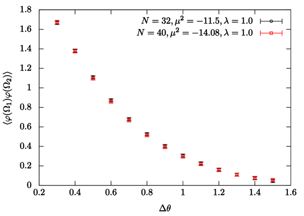
Figure 6: $\left\langle\varphi(\Omega_{1})\varphi(\Omega_{2})\right\rangle$ at $N=32$, $\mu^{2}=-11.5$ and $\lambda=1.0$ is plotted against $\Delta\theta$, where the data are represented by the circles $\zeta_{40\rightarrow 32}\left\langle\varphi(\Omega_{1})\varphi(\Omega_{2})\right\rangle$ with $\zeta_{40\rightarrow 32}=0.8617$ at $N=40$, $\mu^{2}=-14.08$ and $\lambda=1.0$ is also plotted against $\Delta\theta$, where the data are represented by the squares.

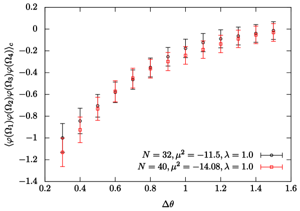
Figure 7: $\left\langle\varphi(\Omega_{1})\varphi(\Omega_{2})\varphi(\Omega_{3})\varphi(\Omega_{4})\right\rangle_{c}$ at $N=32$, $\mu^{2}=-11.5$ and $\lambda=1.0$ is plotted against $\Delta\theta$, where the data are represented by the circles. $\zeta_{40\rightarrow 32}^{2}\left\langle\varphi(\Omega_{1})\varphi(\Omega_{2})\varphi(\Omega_{3})\varphi(\Omega_{4})\right\rangle_{c}$ with $\zeta_{40\rightarrow 32}^{2}=0.7425$ at $N=40$, $\mu^{2}=-14.08$ and $\lambda=1.0$ is also plotted against $\Delta\theta$, where the data are represented by the squares.

3.3 One-parameter fine tuning

In the previous subsection, fixing $\lambda$ and changing the UV cutoff $N$, we tuned $\mu^{2}$ depending on $N$ to perform the renormalization. The results suggest that tuning a parameter specifies a theory. Thus we expect that by fixing $N$ and changing $\lambda$ one obtains the same theory by tuning $\mu^{2}$ depending on $\lambda$.

In this subsection, we see that this is indeed the case. We simulate at various values of $\mu^{2}$, $\lambda=0.75$ and $N=32$, and compare the results with thoes at $\mu^{2}=-11.5$, $\lambda=1.0$ and $N=32$. In Fig.8, we plot the logarithm of the 2-point functions at $\mu^{2}=-11.5$ and $\lambda=1.0$ and at typical values of $\mu^{2}$, $-7.7,-11.5,-5.0$, and $\lambda=0.75$. We find that the data for $\mu^{2}=-7.7$ and $\lambda=0.75$ agree with those for $\mu^{2}=-11.5$ and $\lambda=1.0$ if the former are simultaneously shifted in the vertical direction. By using the least-squares method, we determine that $\alpha_{0.75\rightarrow 1.0}=\log(Z(\lambda=1.0)/Z(\lambda=0.75))$. Correspondingly, we obtain $\zeta_{0.75\rightarrow 1.0}=e^{\alpha_{0.75\rightarrow 1.0}}=Z(\lambda=1.0)/Z(\lambda=0.75)$. The values of $\alpha$ and $\zeta$ that we have determined are summarized in Table2.

In Fig.9, we see that the 2-point function at $\mu^{2}=-7.7$ and $\lambda=0.75$ multiplied by $\zeta_{0.75\rightarrow 1.0}$ agrees with that at $\mu^{2}=-11.5$ and $\lambda=1.0$. In Fig.10, we also see that the connected 4-point function at $\mu^{2}=-7.7$ and $\lambda=0.75$ multiplied by $\zeta_{0.75\rightarrow 1.0}^{2}$ agrees with that at $\mu^{2}=-11.5$ and $\lambda=1.0$. These results strongly suggest that the theory at $N=32$, $\mu^{2}=-7.7$ and $\lambda=0.75$ is the same as that at $N=32$, $\mu^{2}=-11.5$ and $\lambda=1.0$ and that our conjecture that a theory is specified by tuning a parameter is valid.

$\lambda^{\prime}\rightarrow\lambda$	$\alpha_{\lambda^{\prime}\rightarrow\lambda}$	$\delta\alpha_{\lambda^{\prime}\rightarrow\lambda}$	$\zeta_{\lambda^{\prime}\rightarrow\lambda}$	$\zeta_{\lambda^{\prime}\rightarrow\lambda}^{2}$
$0.75\rightarrow 1.0$	$0.02426$	$0.01086$	$1.025$	$1.051$

Table 2: $\alpha_{\lambda^{\prime}\rightarrow\lambda}$, $\delta\alpha_{\lambda^{\prime}\rightarrow\lambda}$, $\zeta_{\lambda^{\prime}\rightarrow\lambda}$ and $\zeta_{\lambda^{\prime}\rightarrow\lambda}^{2}$ ($N=32$).

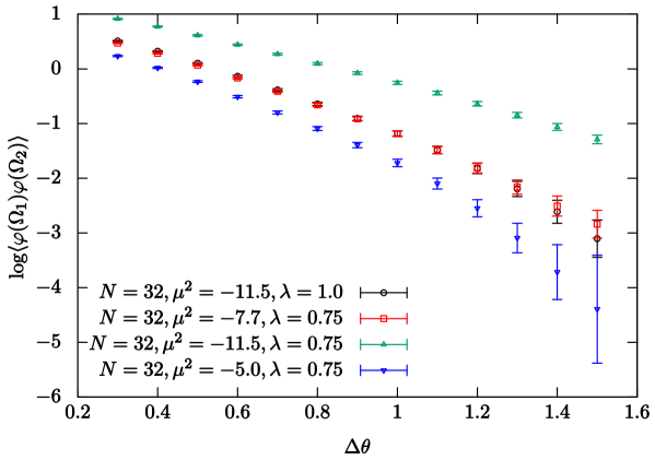
Figure 8: $\log\left\langle\varphi(\Omega_{1})\varphi(\Omega_{2})\right\rangle$ at $N=32$ is plotted against $\Delta\theta$. The data for $\mu^{2}=-11.5$ and $\lambda=1.0$ are represented by the circles, while the data for $\mu^{2}=-7.7,-11.5,-5.0$ and $\lambda=0.75$ are represented by the squares, the triangles and the inverted triangles, respectively.

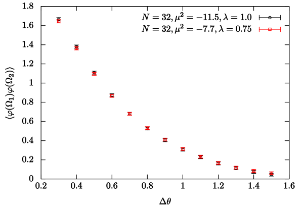
Figure 9: $\left\langle\varphi(\Omega_{1})\varphi(\Omega_{2})\right\rangle$ at $N=32$, $\mu^{2}=-11.5$ and $\lambda=1.0$ is plotted against $\Delta\theta$, where the data are represented by the circles. $\zeta_{0.75\rightarrow 1.0}\left\langle\varphi(\Omega_{1})\varphi(\Omega_{2})\right\rangle$ with $\zeta_{0.75\rightarrow 1.0}=1.025$ at $N=32$, $\mu^{2}=-7.7$ and $\lambda=0.75$ is also plotted against $\Delta\theta$, where the data are represented by the squares.

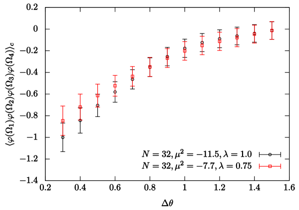
Figure 10: $\left\langle\varphi(\Omega_{1})\varphi(\Omega_{2})\varphi(\Omega_{3})\varphi(\Omega_{4})\right\rangle_{c}$ at $N=32$, $\mu^{2}=-11.5$ and $\lambda=1.0$ is plotted against $\Delta\theta$, where the data are represented by the circles. $\zeta_{0.75\rightarrow 1.0}^{2}\left\langle\varphi(\Omega_{1})\varphi(\Omega_{2})\varphi(\Omega_{3})\varphi(\Omega_{4})\right\rangle_{c}$ with $\zeta_{0.75\rightarrow 1.0}^{2}=1.051$ at $N=32$, $\mu^{2}=-7.7$ and $\lambda=0.75$ is also plotted against $\Delta\theta$, where the data are represented by the squares.

4 Conclusion and discussion

In this paper, we have studied nonperturbative renormalization in a scalar field theory on the fuzzy sphere by calculating the correlation functions by Monte Carlo simulation. The theory is realized by a matrix model, where the matrix size plays the role of the UV cutoff, and the Berezin symbol constructed from the coherent state is identified with the field. We found that the 2-point and connected 4-point functions are made independent of the matrix size by tuning a parameter and performing the wave function renormalization. Thus the results strongly suggest that the theory is nonperturbatively renormalized in the ordinary manner and that the theory is fixed by tuning a parameter. To support the latter statement, we examined the correlation functions at fixed $N$. We found that two different sets of $(\mu^{2},\lambda)$ indeed give the same theory.

We omitted data for the values of $\Delta\theta$ less than 0.3. We found that the agreement for $\Delta\theta<0.3$ between the correlation functions is not so good as that for $\Delta\theta\geq 0.3$ while the data for $\Delta\theta<0.3$ in the correlation functions that we compare are very close. This should be attributed to the effect of the finite UV cutoff, $N$. We expect the slight deviation for $\Delta\theta<0.3$ to vanish in $N\rightarrow\infty$.

Now let us see that the $N$ dependence of $\mu^{2}$ with $\lambda$ fixed is approximately given by

$$\mu^{2}=\tilde{\mu}^{2}-c\log N\ .$$ (4.1)

By applying $(\mu^{2},N)=(-7.97,24),(-11.5,32)$ to this equation, we obtain

$$\tilde{\mu}^{2}=31.0,\;\;\;c=12.3\ .$$ (4.2)

Substituting $N=40$ into (4.1) with the above values of $\tilde{\mu}^{2}$ and $c$ yields

$$\mu^{2}=-14.4\ ,$$ (4.3)

which is close to $-14.08$ that we adopted for $N=40$. Thus there should be a correction to (4.1) that vanishes in the $N\rightarrow\infty$ limit. On the other hand, the one-loop calculation of the self-energy in [9, 10] gives $c=6\lambda=6.0$. Hence, our renormalization is indeed a nonperturbative one. To fix the $N$ dependence of $Z$, we need to further simulate at other $N$’s.

The theory that we have obtained is considered to be a finite-volume and noncommutative analog of the $\lambda\phi^{4}$ theory in $R^{2}$, which is obtained by tuning a parameter and which belongs to the same universality class as the 2d Ising model (see, for example, [40, 41].). We should reveal the differences between our theory and an $S^{2}$ analog of the $\lambda\phi^{4}$ theory in $R^{2}$, whose action is given by (2.1), by calculating the correlation functions in the latter theory and comparing them with thoes that we have obtained in this paper. Namely, it is important to elucidate how noncommutativity or nonlocality affects the correlation functions.

It is shown in [11, 12, 13, 14, 15] that there are three phases in the matrix model (2.3): the disordered, uniformly ordered and striped phases [42, 43]. As we showed in appendix B, the 1-point functions vanish. This implies that the theory that we have obtained is in the disordered phase. Indeed, the parameters $\mu^{2}$ and $\lambda$ that we have used in this paper are consistent with the disordered phase. We would like to examine renormalization in the other phases. For this purpose, it seems that we need to study a different scaling limit rather than the commutative limit. To investigate nonperturbative renormalization in gauge theories on the fuzzy sphere should also be important.

To study the above issues, it should be useful to use to other methods such as the renormalization group analysis developed in [16] as well as Monte Carlo simulation.

We hope to report on a study of the above issues in the near future.

Appendix A: Bloch coherent state and Berezin symbol

In this appendix, we review the Bloch coherent state [30], the Berezin symbol[29] and the star product on the fuzzy sphere.

We use a standard basis $|jm\rangle$ $(m=-j,-j+1,\dots,j)$ for the spin $j$ representation of the $SU(2)$ algebra, which obeys the relations

$$L_{\pm}|jm\rangle =\sqrt{(j\mp m)(j\pm m+1)}|jm\pm 1\rangle,$$

$$L_{3}|jm\rangle =m|jm\rangle\ ,$$ (A.1)

where $L_{\pm}=L_{1}\pm iL_{2}$. The state $|jj\rangle$ is interpreted as corresponding to the north pole on the sphere. Then, the state $|\Omega\rangle$ corresponding to a point $\Omega=(\theta,\varphi)$ is obtained by multiplying $|jj\rangle$ by a rotation operator as

$$|\Omega\rangle=e^{i\theta(\sin\varphi L_{1}-\cos\varphi L_{2})}|jj\rangle\ .$$ (A.2)

The state $|\Omega\rangle$ is called the Bloch coherent state. It follows from (A.2) that

$$n_{i}L_{i}|\Omega\rangle=j|\Omega\rangle\ ,$$ (A.3)

where $\vec{n}=(\sin\theta\cos\varphi,\sin\theta\sin\varphi,\cos\theta)$. (A.3) implies that the states $|\Omega\rangle$ minimize $\sum_{i}(\Delta L_{i})^{2}$, where $(\Delta L_{i})^{2}$ is the standard deviation of $L_{i}$.

Here we introduce the stereographic projection given by $z=\tan\frac{\theta}{2}e^{i\varphi}$. Then, (A.2) is expressed as

$$|\Omega\rangle=e^{zL_{-}}e^{-L_{3}\log(1+|z|^{2})}e^{-\bar{z}L_{+}}|jj\rangle\ .$$ (A.4)

By using (A.4), an explicit form of $|\Omega\rangle$ is obtained as

$$|\Omega\rangle=\sum_{m=-j}^{j}\left(\begin{array}[]{c}2j\\ j+m\end{array}\right)^{\frac{1}{2}}\left(\cos\frac{\theta}{2}\right)^{j+m}\left(\sin\frac{\theta}{2}\right)^{j-m}e^{i(j-m)\varphi}|jm\rangle\ .$$ (A.7)

By using (A.7), it is easy to show the following relations:

$$\langle\Omega_{1}|\Omega_{2}\rangle=\left(\cos\frac{\theta_{1}}{2}\cos\frac{\theta_{2}}{2}+e^{i(\varphi_{2}-\varphi_{1})}\sin\frac{\theta_{1}}{2}\sin\frac{\theta_{2}}{2}\right)^{2j}\ ,$$ (A.8)

$$|\langle\Omega_{1}|\Omega_{2}\rangle|=\left(\cos\frac{\chi}{2}\right)^{2j}\;\;\mbox{with}\;\;\chi=\arccos(\vec{n}_{1}\cdot\vec{n}_{2})\ ,$$ (A.9)

$$\frac{2j+1}{4\pi}\int d\Omega\ |\Omega\rangle\langle\Omega|=1\ .$$ (A.10)

Putting $\chi=\frac{2}{\sqrt{j}}$ in the RHS of (A.9) yields

$$\left(\cos\frac{\chi}{2}\right)^{2j}\approx\left(1-\frac{1}{2j}\right)^{2j}\approx e^{-1}$$ (A.11)

for large $j$. This implies that the effective width of the Bloch coherent state is given by $\frac{R}{\sqrt{j}}=\frac{1}{\sqrt{j}}$.

We also denote the Bloch coherent state $|\Omega\rangle$ by $|z\rangle$. (A.7) and (A.10) are rewritten as

$$|z\rangle=\left(\frac{z}{1+|z|^{2}}\right)^{j}\sum_{m=-j}^{j}\left(\begin{array}[]{c}2j\\ j+m\end{array}\right)^{\frac{1}{2}}\frac{1}{z^{m}}|jm\rangle\ ,$$ (A.14)

$$\frac{2j+1}{4\pi}4\int\frac{d^{2}z}{(1+|z|^{2})^{2}}\ |z\rangle\langle z|=1\ ,$$ (A.15)

respectively.

The Berezin symbol for a $(2j+1)\times(2j+1)$ matrix $A$ is defined by

$$f_{A}(\Omega) =f_{A}(z,\bar{z})$$

$$=\langle\Omega|A|\Omega\rangle$$

$$=\langle z|A|z\rangle\ .$$ (A.16)

The star product for $A$ and $B$ is defined by

$$f_{A}\star f_{B}(\Omega)=f_{A}\star f_{B}(z,\bar{z})=\langle\Omega|AB|\Omega\rangle=\langle z|AB|z\rangle\ .$$ (A.17)

Here we consider a quantity

$$\frac{\langle w|A|z\rangle}{\langle w|z\rangle}\ .$$ (A.18)

(A.14) implies that this quantity is holomorphic with respect to $z$ and anti-holomorphic with respect to $w$. Then, it follows that

$$\frac{\langle w|A|z\rangle}{\langle w|z\rangle} =e^{-w\frac{\partial}{\partial z}}\frac{\langle w|A|z+w\rangle}{\langle w|z+w\rangle}$$

$$=e^{-w\frac{\partial}{\partial z}}e^{z\frac{\partial}{\partial w}}\frac{\langle w|A|w\rangle}{\langle w|w\rangle}$$

$$=e^{-w\frac{\partial}{\partial z}}e^{z\frac{\partial}{\partial w}}\langle w|A|w\rangle$$

$$=e^{-w\frac{\partial}{\partial z}}e^{z\frac{\partial}{\partial w}}f_{A}(w,\bar{w})\ .$$ (A.19)

Similarly,

$$\frac{\langle z|A|w\rangle}{\langle z|w\rangle}=e^{-\bar{w}\frac{\partial}{\partial\bar{z}}}e^{\bar{z}\frac{\partial}{\partial\bar{w}}}f_{A}(w,\bar{w})\ .$$ (A.20)

By using (A.15), (A.19) and (A.20), one can calculate the star product as

$$f_{A}\star f_{B}(w,\bar{w}) =\langle w|AB|w\rangle$$

$$=\frac{2j+1}{4\pi}4\int\frac{d^{2}z}{(1+|z|^{2})^{2}}\frac{\langle w|A|z\rangle}{\langle w|z\rangle}\frac{\langle z|B|w\rangle}{\langle z|w\rangle}|\langle w|z\rangle|^{2}$$

$$=\frac{2j+1}{4\pi}4\int\frac{d^{2}z}{(1+|z|^{2})^{2}}(e^{-w\frac{\partial}{\partial z}}e^{z\frac{\partial}{\partial w}}f_{A}(w,\bar{w}))(e^{-\bar{w}\frac{\partial}{\partial\bar{z}}}e^{\bar{z}\frac{\partial}{\partial\bar{w}}}f_{B}(w,\bar{w}))|\langle w|z\rangle|^{2}\ .$$ (A.21)

Appendix B: One-point functions

In this appendix, we show the results for the 1-point functions. In Fig.11, we plot $\left\langle\varphi(\Omega_{1})\right\rangle$ at $N=32$, $\mu^{2}=-11.5$ and $\lambda=1.0$ against $\Delta\theta$. We see that it vanishes within the error. We have verified that the 1-point functions also vanish for the other cases that we simulate.

Figure 11: $\left\langle\varphi(\Omega_{1})\right\rangle$ at $N=32$, $\mu^{2}=-11.5$ and $\lambda=1.0$ is plotted against $\Delta\theta$.

References

- [1] M. R. Douglas and N. A. Nekrasov, Rev. Mod. Phys. 73, 977 (2001) doi:10.1103/RevModPhys.73.977 [hep-th/0106048].
- [2] A. Connes, M. R. Douglas and A. S. Schwarz, JHEP 9802, 003 (1998) doi:10.1088/1126-6708/1998/02/003 [hep-th/9711162].
- [3] H. Aoki, N. Ishibashi, S. Iso, H. Kawai, Y. Kitazawa and T. Tada, Nucl. Phys. B 565, 176 (2000) doi:10.1016/S0550-3213(99)00633-1 [hep-th/9908141].
- [4] T. Banks, W. Fischler, S. H. Shenker and L. Susskind, Phys. Rev. D 55, 5112 (1997) [hep-th/9610043].
- [5] N. Ishibashi, H. Kawai, Y. Kitazawa and A. Tsuchiya, Nucl. Phys. B 498, 467 (1997) [hep-th/9612115].
- [6] R. Dijkgraaf, E. P. Verlinde and H. L. Verlinde, Nucl. Phys. B 500, 43 (1997) [hep-th/9703030].
- [7] S. Minwalla, M. Van Raamsdonk and N. Seiberg, JHEP 0002, 020 (2000) [hep-th/9912072].
- [8] J. Madore, Class. Quant. Grav. 9, 69 (1992). doi:10.1088/0264-9381/9/1/008
- [9] C. S. Chu, J. Madore and H. Steinacker, JHEP 0108, 038 (2001) [hep-th/0106205].
- [10] H. C. Steinacker, Nucl. Phys. B 910, 346 (2016) doi:10.1016/j.nuclphysb.2016.06.029 [arXiv:1606.00646 [hep-th]].
- [11] X. Martin, JHEP 0404, 077 (2004) doi:10.1088/1126-6708/2004/04/077 [hep-th/0402230].
- [12] M. Panero, JHEP 0705, 082 (2007) doi:10.1088/1126-6708/2007/05/082 [hep-th/0608202].
- [13] M. Panero, SIGMA 2, 081 (2006) doi:10.3842/SIGMA.2006.081 [hep-th/0609205].
- [14] F. Garcia Flores, X. Martin and D. O’Connor, Int. J. Mod. Phys. A 24, 3917 (2009) doi:10.1142/S0217751X09043195 [arXiv:0903.1986 [hep-lat]].
- [15] C. R. Das, S. Digal and T. R. Govindarajan, Mod. Phys. Lett. A 23, 1781 (2008) doi:10.1142/S0217732308025656 [arXiv:0706.0695 [hep-th]].
- [16] S. Kawamoto and T. Kuroki, JHEP 1506, 062 (2015) [arXiv:1503.08411 [hep-th]].
- [17] S. Vaidya and B. Ydri, Nucl. Phys. B 671, 401 (2003) doi:10.1016/j.nuclphysb.2003.08.023 [hep-th/0305201].
- [18] D. O’Connor and C. Saemann, JHEP 0708, 066 (2007) doi:10.1088/1126-6708/2007/08/066 [arXiv:0706.2493 [hep-th]].
- [19] V. P. Nair, A. P. Polychronakos and J. Tekel, Phys. Rev. D 85, 045021 (2012) doi:10.1103/PhysRevD.85.045021 [arXiv:1109.3349 [hep-th]].
- [20] A. P. Polychronakos, Phys. Rev. D 88, 065010 (2013) doi:10.1103/PhysRevD.88.065010 [arXiv:1306.6645 [hep-th]].
- [21] J. Tekel, Phys. Rev. D 87, no. 8, 085015 (2013) doi:10.1103/PhysRevD.87.085015 [arXiv:1301.2154 [hep-th]].
- [22] C. Saemann, JHEP 1504, 044 (2015) doi:10.1007/JHEP04(2015)044 [arXiv:1412.6255 [hep-th]].
- [23] J. Tekel, JHEP 1410, 144 (2014) doi:10.1007/JHEP10(2014)144 [arXiv:1407.4061 [hep-th]].
- [24] J. Tekel, JHEP 1512, 176 (2015) doi:10.1007/JHEP12(2015)176 [arXiv:1510.07496 [hep-th]].
- [25] W. Bietenholz, F. Hofheinz and J. Nishimura, JHEP 0406, 042 (2004) doi:10.1088/1126-6708/2004/06/042 [hep-th/0404020].
- [26] H. Mejía-Díaz, W. Bietenholz and M. Panero, JHEP 1410, 56 (2014) doi:10.1007/JHEP10(2014)056 [arXiv:1403.3318 [hep-lat]].
- [27] W. Bietenholz, F. Hofheinz and J. Nishimura, JHEP 0209, 009 (2002) doi:10.1088/1126-6708/2002/09/009 [hep-th/0203151].
- [28] W. Bietenholz, J. Nishimura, Y. Susaki and J. Volkholz, JHEP 0610, 042 (2006) doi:10.1088/1126-6708/2006/10/042 [hep-th/0608072].
- [29] F. A. Berezin, Commun. Math. Phys. 40, 153 (1975).
- [30] J. P. Gazeau. Coherent states in quantum physics - 2009. Weinheim, Germany: WileyVCH.
- [31] S. Iso, H. Kawai and Y. Kitazawa, Nucl. Phys. B 576, 375 (2000) doi:10.1016/S0550-3213(00)00092-4 [hep-th/0001027].
- [32] S. Okuno, M. Suzuki and A. Tsuchiya, PTEP 2016, no. 2, 023B03 (2016) doi:10.1093/ptep/ptv192 [arXiv:1512.06484 [hep-th]].
- [33] M. Suzuki and A. Tsuchiya, PTEP 2017, no. 4, 043B07 (2017) [arXiv:1611.06336 [hep-th]].
- [34] J. L. Karczmarek and P. Sabella-Garnier, JHEP 1403, 129 (2014) [arXiv:1310.8345 [hep-th]].
- [35] P. Sabella-Garnier, JHEP 1502, 063 (2015) [arXiv:1409.7069 [hep-th]].
- [36] G. Alexanian, A. Pinzul and A. Stern, Nucl. Phys. B 600, 531 (2001) [hep-th/0010187].
- [37] A. B. Hammou, M. Lagraa and M. M. Sheikh-Jabbari, Phys. Rev. D 66, 025025 (2002) [hep-th/0110291].
- [38] P. Presnajder, J. Math. Phys. 41, 2789 (2000) [hep-th/9912050].
- [39] G. Ishiki, Phys. Rev. D 92, no. 4, 046009 (2015) [arXiv:1503.01230 [hep-th]].
- [40] W. Loinaz and R. S. Willey, Phys. Rev. D 58, 076003 (1998) doi:10.1103/PhysRevD.58.076003 [hep-lat/9712008].
- [41] P. Bosetti, B. De Palma and M. Guagnelli, Phys. Rev. D 92, no. 3, 034509 (2015) doi:10.1103/PhysRevD.92.034509 [arXiv:1506.08587 [hep-lat]].
- [42] S. S. Gubser and S. L. Sondhi, Nucl. Phys. B 605, 395 (2001) doi:10.1016/S0550-3213(01)00108-0 [hep-th/0006119].
- [43] J. Ambjorn and S. Catterall, Phys. Lett. B 549, 253 (2002) doi:10.1016/S0370-2693(02)02906-4 [hep-lat/0209106].