[1704.01718] INTRODUCTION

Astronomy Letters, 2017, Vol. 43, No 5, pp. 304–315.

Vertical Distribution and Kinematics of Planetary Nebulae

in the Milky Way

V.V. Bobylev¹¹1e-mail: vbobylev@gao.spb.ru and A.T. Bajkova

Central (Pulkovo) Astronomical Observatory, Russian Academy of Sciences,

Pulkovskoe sh. 65, St. Petersburg, 196140 Russia

Abstract—Based on published data, we have produced a sample of planetary nebulae (PNe) that is complete within 2 kpc of the Sun. We have estimated the total number of PNe in the Galaxy from this sample to be $17000\pm 3000$ and determined the vertical scale height of the thin disk based on an exponential density distribution to be $197\pm 10$ pc. The next sample includes PNe from the Stanghellini–Haywood catalog with minor additions. For this purpose, we have used $\sim$ 200 PNe with Peimbert’s types I, II, and III. In this case, we have obtained a considerably higher value of the vertical scale height that increases noticeably with sample radius. We have experimentally found that it is necessary to reduce the distance scale of this catalog approximately by 20%. Then, for example, for PNe with heliocentric distances less than 4 kpc the vertical scale height is $256\pm 12$ kpc. A kinematic analysis has confirmed the necessity of such a reduction of the distance scale.

INTRODUCTION

Planetary nebulae (PNe) reflect a very short ( $10^{3}-10^{4}$ yr) phase in the evolution of stars with a mass of $1-9M_{\odot}.$ This phase begins when an asymptotic giant branch (AGB) star ejects its envelope and ends with the formation of a white dwarf. PNe in the Galaxy are represented everywhere, in the thin and thick disks, in the halo and the bulge, of course, in different proportions. Therefore, PNe are an important source of information about the structure of the Galaxy, its chemical and dynamical evolution.

More than 1500 PNe have been discovered in the Galaxy to date. However, the estimates of their total number $N_{tot}$ differ significantly, from $4\times 10^{3}$ to $4\times 10^{5}:$ 4000–22 000 (Alloin et al. 1976), $10000\pm 4000$ (Jacoby 1980), 40000 (Amnuel et al. 1984), $>10^{5}$ (Ishida and Weinberger 1987), $(2-4)\times 10^{5}$ (Khromov 1989), $7200\pm 1800$ (Peimbert 1990), $23000\pm 6000$ (Zijlstra and Pottasch 1991), $46000\pm 13000$ (Moe and Marco 2006), or $24000\pm 4000$ (Frew 2008).

At present, there are measurements of the trigonometric parallaxes for the central stars of PNe. Such measurements at optical wavelengths have been performed on the basis of observations from the ground (Harris et al. 2007) and spacecraft, in particular, the Hubble Space Telescope (Benedict et al. 2009) and the Gaia satellite (Gaia Collaboration, Prusti et al. 2016). The trigonometric parallaxes of several PNe have also been measured with ground-based very-long-baseline interferometers, in particular, the parallax of the PN K 3–35 was measured within the Japanese VERA (VLBI Exploration of Radio Astrometry) Program (Tafoya et al. 2011). As Stanghellini et al. (2016) showed, in the first published Gaia Data Release (DR1, Gaia Collaboration, Brown et al. 2016) the parallaxes of only seven PNe have been measured so far with a relative error $<80\%.$ Of course, upon completion of the satellite flight the number of reliably measured parallaxes for PNe will increase several-fold.

Since highly accurate (with an error of 10–15%) parallax measurements cover very few PNe, the distances to these objects are usually estimated by various indirect methods. In particular, the statistical method by Shklovskii (1956), which is based on an empirical relation between the ionized mass in the shell and its radius, is widely used. In this case, the errors in the distances are fairly large. An overview of the methods and a comparison of various PN distance scales can be found in Smith (2015).

The Galactic disk is a complex formation that contains stars of various ages belonging to various dynamical structures. It is customary to divide it into the thin and thick disks by either spatial or kinematic criteria. Several models of the Galaxy with fixed values of, for example, the densities, the radial scale lengths or scale heights for each disk have been constructed with such an approach (Robin et al. 2003; Girardi et al. 2005). A more complex approach suggesting that the disk consists of a multitude of independently evolving structures, each having elemental abundances in a very narrow range of values, has been developed in recent years (Rix and Bovy 2013; Bovy et al. 2016). From this viewpoint, analyzing the spatial distribution of such highly specialized objects as PNe is of great interest.

The goal of this paper is to study the $z$ distribution and kinematics of PNe in the Galaxy. This suggests solving the following problems: producing a complete sample, estimating the vertical disk scale height, estimating the total number of PNe in the Galaxy, and studying the vertical distribution and kinematics of PNe based on a sample from a wide solar neighborhood.

METHODS

Vertical Distribution of Galactic Objects

We use the heliocentric rectangular $xyz$ coordinate system where the $x$ axis is directed toward the Galactic center, the $y$ axis is in the direction of Galactic rotation, and the $z$ axis is directed to the north Galactic pole. The heliocentric distance is $r^{2}=x^{2}+y^{2}+z^{2}$ and the cylindrical radius is $d^{2}_{xy}=x^{2}+y^{2}.$

The observed frequency distribution of objects along the $z$ coordinate axis is described by expressions of the following from in the model of an exponential density distribution:

N(z)=N_{1}\exp\biggl{(}-{|z-z_{\odot}|\over h_{1}}\biggr{)},

(1)

where $N_{1}$ is the normalization coefficient, $z_{\odot}$ is the distance from the Sun to the Galactic midplane (the mean of the $z$ coordinates of all objects from the sample), and $h_{1}$ is the vertical disk scale height; in the model of a self-gravitating isothermal disk (Conti and Vacca 1990)

N(z)=N_{2}{\hbox{ sech}}^{2}\biggl{(}{z-z_{\odot}\over\sqrt{2}\leavevmode\nobreak\ h_{2}}\biggr{)},

(2)

where $N_{2}$ is the normalization coefficient, $h_{2}$ is the vertical disk scale height; and, finally, in the Gaussian model

N(z)=N_{3}\exp\biggl{[}-{1\over 2}\biggl{(}{z-z_{\odot}\over h_{3}}\biggr{)}^{2}\biggr{]},

(3)

where $N_{3}$ is the normalization coefficient. Although the standard of the normal distribution $h_{3}$ in the strict sense (this term is usually applicable to exponential laws) is not a parameter of the vertical scale height, here we attach this meaning to it.

To estimate the total number of objects in the Galaxy $N_{tot},$ we use the following relation (Piskunov et al. 2006):

N_{tot}=2\pi\Sigma_{xy}\int^{R^{lim}}_{0}\exp\biggl{(}-{R-R_{\odot}\over L_{d}}\biggr{)}RdR,

(4)

where $R$ is the projection of the distance from the star to the Galactic center onto the Galactic $xy$ plane; $R^{lim}$ is the Galactocentric radius of the disk; $L_{d}$ is the radial disk scale length; $\Sigma_{xy}=N_{f}/(\pi d^{2}_{xy})$ is the surface density in the solar neighborhood found under the condition of sample completeness, where $d_{xy}$ is the sample completeness radius in the $xy$ plane and $N_{f}$ is the number of objects in the sample. We take $R^{lim}=15$ kpc, $L_{d}=3.5$ kpc, and $R_{\odot}=8$ kpc, which correspond to the model from Bahcall and Soneira (1980).

Kinematics

To determine the parameters of the Galactic rotation curve, we use the equations derived from Bottlinger’s formulas in which the angular velocity $\Omega$ is expanded into a series to terms of the second order of smallness in $r/R_{0}:$

\begin{array}[]{lll}V_{r}=-U_{\odot}\cos b\cos l-V_{\odot}\cos b\sin l-W_{\odot}\sin b+\\ +R_{0}(R-R_{0})\sin l\cos b\Omega^{{}^{\prime}}_{0}+0.5R_{0}(R-R_{0})^{2}\sin l\cos b\Omega^{{}^{\prime\prime}}_{0},\end{array}

(5)

\begin{array}[]{lll}V_{l}=U_{\odot}\sin l-V_{\odot}\cos l-r\Omega_{0}\cos b+\\ +(R-R_{0})(R_{0}\cos l-r\cos b)\Omega^{{}^{\prime}}_{0}+0.5(R-R_{0})^{2}(R_{0}\cos l-r\cos b)\Omega^{{}^{\prime\prime}}_{0},\end{array}

(6)

\begin{array}[]{lll}V_{b}=U_{\odot}\cos l\sin b+V_{\odot}\sin l\sin b-W_{\odot}\cos b-\\ -R_{0}(R-R_{0})\sin l\sin b\Omega^{{}^{\prime}}_{0}-0.5R_{0}(R-R_{0})^{2}\sin l\sin b\Omega^{{}^{\prime\prime}}_{0},\end{array}

(7)

where $U_{\odot},V_{\odot},W_{\odot}$ are the components of the group velocity vector for the stars being considered relative to the local standard of rest (taken with the opposite sign), $R$ is the distance from the star to the Galactic rotation axis:

R^{2}=r^{2}\cos^{2}b-2R_{0}r\cos b\cos l+R^{2}_{0}.

(8)

$\Omega_{0}$ is the angular velocity of Galactic rotation at the Galactocentric distance $R_{0}$ of the Sun, the parameters $\Omega^{{}^{\prime}}_{0}$ and $\Omega^{{}^{\prime\prime}}$ are the corresponding derivatives of the angular velocity, $V_{0}=|R_{0}\Omega_{0}|$ . The velocities $V_{R}$ and $\Delta V_{circ}$ must be freed from the peculiar solar velocity $U_{\odot},V_{\odot},W_{\odot}$ .

It is important to know the specific value of the distance R0. Gillessen et al. (2009) obtained one of its most reliable estimates, $R_{0}=8.28\pm 0.29$ kpc, by analyzing the orbits of stars moving around the massive black hole at the Galactic center. The following estimates were obtained from various samples of masers with measured trigonometric parallaxes: $R_{0}=8.34\pm 0.16$ kpc (Reid et al. 2014), $8.3\pm 0.2$ kpc (Bobylev and Bajkova 2014), $8.03\pm 0.12$ kpc (Bajkova and Bobylev 2015), and $8.40\pm 0.12$ kpc (Rastorguev et al. 2016). Based on these results, we adopted $R_{0}=8.3\pm 0.2$ kpc in this paper.

Note that we apply the kinematic equations (5)–(7) to the PNe that are involved in the Galactic rotation. Therefore, we seek to maximally free the sample from the noise introduced, for example, by the halo objects that are no involved in this rotation.

DATA

The catalog by Stanghellini and Haywood (2010), which contains 728 PNe with distance estimates, served as one of the data sources for our study. It is one of the largest catalogs of PNe with homogeneous distance estimates to date. For example, the bibliographic compilation by Acker et al. (1992) contains only 296 PNe with more or less reliable distance estimates obtained by various methods. The catalog by Phillips (2004) numbers already 447 such nebulae. A historical background on the catalogs of PNe can be found, for example, in Parker et al. (2006). PNe from the catalog by Stanghellini and Haywood (2010) cover much of the Galaxy; the heliocentric distances of some of them exceed 20 kpc.

In the catalog by Stanghellini and Haywood (2010) the distances to PNe were estimated using a statistical method (Cahn et al. 1992; Stanghellini et al. 2008). Data on the radio flux from observations at a frequency of 5 GHz are used to calculate the mass of the ionized shell. It is important to note two facts. First, the catalog by Stanghellini and Haywood (2010) contains a fairly homogeneous material in which only a few bipolar nebulae poorly follow the PN mass–radius relations. Second, the distance scale was calibrated on the basis of PNe from the Magellanic Clouds. According to the estimate by Stanghellini et al. (2008), the distances are determined in this way with a relative error of $\sim$ 30%. The actual error of these distance estimates can be larger. As a comparative analysis by Smith (2015) showed, the individual distance estimates for PNe could differ by a factor of 2–2.5.

Refer to caption — Рис. 1: Distances to PNe from the catalog by Stanghellini and Haywood (2010) versus their distances from the catalog by Frew (2008).

Таблица 1: Parameters

z_{\odot}

and

h_{i},

i=1,2,3,

found in this paper from the samples of PNe with Peimbert’s types I, II, and III

$z_{\odot},$ pc	$h_{1},$ pc	$h_{2},$ pc	$h_{3},$ pc	Sample	$N_{\star}$
$\leavevmode\nobreak\ -6\pm 7\leavevmode\nobreak\$	$197\pm 10$	$168\pm 7\leavevmode\nobreak\$	$196\pm 9\leavevmode\nobreak\$	sample I, $d_{xy}<2$ kpc	230
$-22\pm 14$	$203\pm 22$	$163\pm 14$	$186\pm 17$	sample II, $r<2.0$ kpc	55
$-13\pm 14$	$271\pm 20$	$245\pm 18$	$291\pm 22$	sample II, $r<3.0$ kpc	94
$-37\pm 12$	$316\pm 15$	$286\pm 15$	$337\pm 18$	sample II, $r<4.0$ kpc	131
$-57\pm 11$	$339\pm 14$	$299\pm 14$	$349\pm 17$	sample II, $r<5.0$ kpc	160
$-84\pm 11$	$382\pm 13$	$325\pm 12$	$376\pm 15$	sample II, $r<6.0$ kpc	199
$-23\pm 14$	$193\pm 22$	$155\pm 14$	$177\pm 17$	sample II, $r<2.0$ kpc	55
$-10\pm 11$	$221\pm 16$	$201\pm 14$	$239\pm 18$	sample II, $r<3.0$ kpc	94
$-40\pm 9\leavevmode\nobreak\$	$256\pm 12$	$232\pm 12$	$275\pm 15$	sample II, $r<4.0$ kpc	131
$-45\pm 9\leavevmode\nobreak\$	$283\pm 14$	$247\pm 11$	$287\pm 13$	sample II, $r<5.0$ kpc	160
$-67\pm 9\leavevmode\nobreak\$	$305\pm 14$	$265\pm 10$	$306\pm 12$	sample II, $r<6.0$ kpc	199

To study the kinematic properties of PNe, we used the line-of-sight velocities and proper motions gathered from various published sources using the SIMBAD electronic database. Note that the proper motions are available only for a small fraction of the catalog, and they were taken mainly from such catalogs as Hipparcos (1997), Tycho-2 (Høg et al. 2000), and UCAC4 (Zacharias et al. 2013). For 16 PNe the proper motions were taken from the first published Gaia Data Release (DR1) (Gaia Collaboration, Brown et al. 2016).

The catalog by Frew (2008) with distance estimates for PNe is of great interest. A comparative analysis by Smith (2015) showed its high quality. It contains more than 200 PNe within $\sim$ 2 kpc of the Sun. Initially, they produced a calibration sample of 120 PNe whose distances were estimated by several methods; subsequently, the remaining observations were tied to this sample. The distances to the remaining nebulae were determined by a statistical method based on an empirical $H\alpha$ surface brightness–radius relation (Frew and Parker 2006; Frew et al. 2013). This relation was calibrated on the basis of PNe from the Magellanic Clouds. According to the estimate by Frew (2008), the distances determined by this method have a relative error of $\sim$ 22% for highly excited shells.

For several PNe we used more reliable distance estimates (with a relative error of less than 20These include NGC 6853, NGC 7293, Abell 31, and DeHt 5 whose trigonometric parallaxes were measured on the basis of Hubble Space Telescope observations (Benedict et al. 2009). For the PNe K 3–35 (Tafoya et al. 2011) and IRAS 1828–095 (Imai et al. 2013) we used the trigonometric parallaxes that were determined from VLBI observations within the Japanese VERA Program. In addition, we used the ground-based optical determinations of the trigonometric parallaxes for ten PNe from Harris et al. (2007): NGC 6720, Abell 74, HDW 4, SH 2–216, PuWe 1, Ton 320, Abell 21, Abell 7, Abell 24, and PG 1034+001.

Note that the SIMBAD database provides evidence (with the corresponding bibliographic references) that some of the objects in the list by Stanghellini and Haywood (2010) are not PNe. For example, G097.5+03.1, G093.5+01.4, G298.1–00.7, and G328.9–02.4 are HII regions, G125.9–47.0 is a star, G173.7–05.8 is a reflection nebula, and G104.8–06.7 and G330.7+04.1 are emission line stars. According to Frew et al. (2013), two stars from the list by Harris et al. (2007), namely RE 1738+665 and PHL 932, are not PNe. We excluded all these objects from consideration.

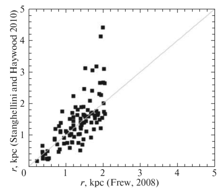
In Fig. 1 the distances to PNe in the scale of Stanghellini and Haywood (2010) are plotted against the distances in the scale of Frew (2008). The lopsided distribution of points at large distances is explained by the fact that there are no nebulae with distances of more than about 2.2 kpc in the catalog by Frew (2008). It can be surmised that if distant objects were present in the catalog by Frew (2008), then the distribution could be symmetric relative to the diagonal plotted in the figure. Such a symmetry is observed at least up to 2 kpc.

For the subsequent work we produced sample I with completeness. It consists of the catalog by Frew (2008) to which we added the above nebulae with measured trigonometric parallaxes and the nebulae from the catalog by Stanghellini and Haywood (2010). A total of 29 nearby ( $r<2$ kpc) nebulae were added to the catalog by Frew (2008). Sample I contains a total of 230 objects no farther than 2 kpc from the Sun.

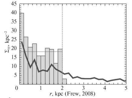
Figure 2 shows the surface density distribution $\sum_{xy}$ of PNe as a function of distance $d_{xy}=r\cos b$ . Based on this graph, we assumed sample I to be complete up to distances of 2.0 kpc and the mean surface density $\sum_{xy}$ to be 18.3 kpc ${}^{-2}.$

Figure 2 also shows the surface density distribution of PNe from the catalog by Stanghellini and Haywood (2010) without any additions. As can be seen from the figure, the catalog by Stanghellini and Haywood (2010) loses to sample I with regard to completeness. However, the catalog by Stanghellini and Haywood (2010) has a big advantage: it has many stars at large distances. For the above nebulae with measured trigonometric parallaxes we took the distances calculated from the parallaxes, took into account the misclassified nebulae, and called this sample II. Sample II contains a total of 726 PNe.

To assign the PNe to particular Galactic subsystems, it is convenient to use the classification introduced by Peimbert (1978) and improved by Quireza et al. (2007). The nebulae of Peimbert’s types I, II, III, IV, and V belong to the thin disk, the thick disk, the halo, and the bulge, respectively. For example, according to Table 5 from Milanova and Kholtygin (2009), the scale height for PNe of different types changes from $\sim$ 0.2 kpc for type I to $\sim$ 1 kpc for type III and $\sim$ 1–2 kpc for type IV. We took the values of the types from Quireza et al. (2007). However, it turned out that information about the PN types according to Peimbert’s classification is available only for 60% of the PNe from the list by Stanghellini and Haywood (2010).

Note that due to the presence of PNe of different types in our sample II, the scale heights $h_{1},h_{2},$ and $h_{3}$ can increase with sample radius $r,$ because old halo objects fall into the sample.

RESULTS AND DISCUSSION

Using our complete sample I with parameters $d_{xy}=2.0$ kpc, $N_{f}=230,$ and $\sum_{xy}=18.3$ kpc^-2 based on Eq. (4), we estimate the total number of PNe in the Galaxy to be $N_{tot}=14929\pm 2850.$

Table 1 gives the parameters $z_{\odot}$ and $h_{i}(i=1,2,3)$ found from samples I and II. For sample I we used the additional constraint $|z|<1.8$ kpc. Several solutions obtained with various constraints on the radius $r$ are given in the case of analyzing sample II. For sample II we used the additional constraint $|z|<2.0$ kpc. Here, we use only those PNe from sample II that have Peimbert’s types I, IIa, IIb, and III. In our sample there are very few type III nebulae that, according to this classification, belong to the thick disk, no more than ten.

The errors of the sought–for parameters were estimated through statistical Monte Carlo simulations. The error estimates were made by generating 1000 random realizations. The measurement errors were added to the distances; we assumed the random errors of the distances in the catalog by Frew (2008) to be 30%.

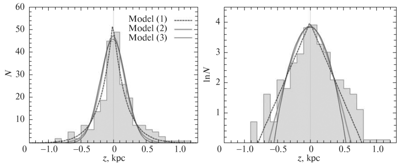
The histogram of the $z$ distribution constructed using sample I is shown in Fig. 3 in both linear and logarithmic scales. Figure 3 displays three curves constructed on the basis of models (1)–(3). As can be seen from the figure, models (2) and (3) describe the broad wings of the distribution more poorly than does model (1).

Note that Zijlstra and Pottasch (1991) used three density distributions to determine the scale height based on PNe. These authors found relations between the scale heights slightly different from ours: $h_{1}=250$ pc, $h_{2}=380/\sqrt{2}=269$ pc (given their modification of the law (2)), and $h_{3}=490$ pc. We agree with the conclusions by Zijlstra and Pottasch (1991) that (1) is the best law to analyze the vertical distribution of PNe.

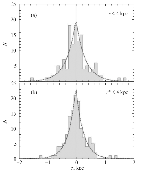
There is a considerable growth of h with sample radius for the PNe from sample II that is difficult to explain. As can be seen from Table 1, for the sample from the range $r<6.0$ kpc the scale height reaches $h_{1}=382$ kpc. Such a value is already typical of thick disk objects. There is no reason to assume that the admixture of PNe from the thick disk and the halo increases considerably with distance in this sample. One of the solutions of this problem is to reduce the distance scale of the catalog by Stanghellini and Haywood (2010). We experimentally found that it would suffice to reduce the distance scale approximately by 20% to obtain acceptable results. The results of such an approach are presented in the lower part of Table 2 and in Figs. 4 and 5. For this purpose, the distance to each star was scaled, and the entire histogram was constructed again, the distances to the nebulae with measured trigonometric parallaxes did not change.

Figure 4 provides the histograms constructed from the data of Table 2 for the PNe of sample II with Peimbert’s types I, II, and III selected under the condition $r<4$ kpc. These histograms were constructed using both the original distances and those multiplied by a factor of 0.8. The curves according to an exponential law were fitted. As can be seen from the figure, reducing the distances leads to a significant improvement of the histogram shape.

In Fig. 5 the scale height $h_{2}$ is plotted against the heliocentric distance $r.$ The values of $h_{2}$ were taken from Table 1. We chose precisely $h_{2},$ because their values are determined with smaller random errors than those of $h_{1}$ and $h_{3}.$ It can be clearly seen from this figure that a relatively small reduction of the distance scale from Stanghellini and Haywood (2010) causes the distance dependence of $h$ to decrease (the slope of the curve to decrease).

The Number of PNe in the Galaxy

Using the parameters $L_{d}=3.3$ kpc and $R^{lim}=15.0$ kpc close to those that we use with the surface density $\sum_{xy}=23.4$ kpc^-2 found, Frew (2008) determined $N_{tot}=19800\pm 4000.$ The value of $N_{tot}=14929\pm 2850$ we found (essentially based on his catalog with minor additions) is consistent with its estimate by Frew (2008) within $1\sigma.$ The existing difference is explained mainly by the difference in the surface densities $\sum_{xy}$ determined by different methods. However, according to Frew (2008), one might also expect a larger number of PNe in the Galaxy, $N_{tot}=24000\pm 4000.$ Such a value was obtained by taking into account the fact that the surface density of PNe increases in the Galactic bulge region.

Following the approach of Frew (2008), we increased our estimate of the total number of PNe by 2000, which takes into account the density rise in the Galactic bulge. As a result, we obtained $N_{tot}=16929\pm 2850.$

Таблица 2: Parameters

z_{\odot}

and

h_{1}

found by various objects from thin-disk objects

$z_{\odot},$ pc	$h_{1},$ pc	Author	Sample
$-24\pm 2$	$\leavevmode\nobreak\ 84\pm 2\leavevmode\nobreak\$	(1)	250 Cepheids, $\sim$ 138 Myr, $r<4$ kpc
$-15\pm 2$	$150\pm 27$	(2)	open clusters, 200–1000 Myr
$0$	$250\pm 50$	(3)	PNe, $r<1$ kpc
$0$	259	(4)	196 PNe
$0$	$217\pm 20$	(5)	PNe, $r<2$ kpc
$0$	$236\pm 10$	(6)	AGB stars, $r<1.4$ kpc
$-27\leavevmode\nobreak\ \leavevmode\nobreak\ \leavevmode\nobreak\ \leavevmode\nobreak\ \leavevmode\nobreak\$	220–300	(7)	717 white dwarfs
$-27\pm 4$	$330\pm 3\leavevmode\nobreak\$	(8)	old thin-disk stars, SDSS
$0$	300	(9)	$M$ dwarfs from SDSS catalog, $r<2$ kpc

(1) Bobylev and Bajkova (2016a), (2) Bonatto et al. (2006), (3) Zijlstra and Pottasch (1991), (4) Corradi and Schwarz (1995), (5) Frew (2008), (6) Olivier et al. (2001),(7) Vennes et al. (2002), (8) Chen et al. (2001), (9) Jurić et al. (2008).

The Scale Height

Table 2 gives a brief overview of $z_{\odot}$ and $h_{1}$ found by various authors from Galactic thin-disk objects. The thin disk is not a homogeneous formation. The first two rows of Table 2 give the estimates obtained from intermediate-age objects. For example, the scale height $h_{1}$ determined from the youngest fraction of the thin disk ranges from $26.5\pm 0.7$ pc for a sample of methanol masers (Bobylev and Bajkova 2016b) to $50\pm 3$ pc (HII regions, Wolf–Rayet stars; Bobylev and Bajkova 2016a).

Bobylev and Bajkova (2016a) found $z_{\odot}$ and $h_{1}$ by analyzing a sample of classical Cepheids with a mean age of 138 Myr. Open star clusters with various ages served as the subject of analysis in Bonatto et al (2006). For the oldest clusters these authors failed to determine the vertical disk scale height. However, Froebrich (2014) showed that for open clusters with an age of more than 1 Gyr the scale height increases sharply ( $h_{1}>200$ pc) and rapidly reaches values that are more typical of thick-disk objects, for example, $h_{1}=550$ pc for clusters with an age of 3.5 Gyr.

The vertical disk scale height has been determined repeatedly by various authors from PNe. Zijlstra and Pottasch (1991) analyzed the vertical distribution of 37 PNe within 1 kpc of the Sun. Corradi and Schwarz (1995) considered a sample of 196 nearby PNe with various morphologies. For example, these authors found the smallest scale height $h_{1}=130$ pc from 35 bipolar nebulae and the largest one $h_{1}=325$ pc from 119 elliptical nebulae. Note that Frew (2008) determined h1 using data on PNe from his catalog with the additional constraint $|z|\leq 300$ pc. Interestingly, we obtained a similar result (sample I) without such a strong constraint.

Olivier et al. (2001) found $h_{1}=236\pm 10$ pc from a sample of 58 AGB stars with medium and high mass loss rates. These stars have masses in the range 1-–2 $M_{\odot}$ and are the direct progenitors of PNe. To estimate the distances to these stars, we used their photometric characteristics in the infrared $JHKL$ bands and the data on their variability.

Based on stars counts for two large samples of stars from the SDSS (Sloan Digital Sky Survey, York et al. 2000) catalog, Chen et al. (2001) constructed models for the thin and thick disks as well as the Galactic halo. Jurić et al. (2008) confirmed the result of Chen et al. (2001) by analyzing a large high-latitude ( $|b|>25^{\circ}$ ) sample of M dwarfs from the SDSS catalog. This catalog is distinguished by a high accuracy of determining the photometric distances of stars. The mean error of the photometric characteristics in it is $\sim$ 0.02 ${}^{m};$ the error in the absolute magnitude $\sigma_{M_{r}}$ is $\sim$ 0.3 ${}^{m}.$ Then, according to the estimate by Jurić et al. (2008), the error in the photometric distances of stars is $\sim$ 18%.

Vennes et al. (2002) studied a sample of 942 spectroscopically identified hydrogen-rich (DA) white dwarfs. They adopted $z_{\odot}=-27$ pc according to the estimate by Chen et al. (2001).

The values of $h_{1}$ presented in Table 2 served us as a guide for choosing the scale factor 0.8 of the distance scale of the catalog by Stanghellini and Haywood (2010). Note that the various distance scales of PNe have been compared by various authors repeatedly (Ortiz 2013; Smith 2015), and a discrepancy between the scales of 20% is encountered quite often.

The vertical scale height $h_{1}=197\pm 10$ pc that we found based on 230 PNe from the combined sample (sample I) is in good agreement with the results of other authors. Note that among the results of the analysis of PNe presented in Table 2, our estimate was obtained from the largest number of nebulae and is distinguished by a high accuracy.

The Galactic Rotation Parameters

We know the various kinematic methods that allow the distance scale factor of the sample being studied to be estimated. A detailed description of several such methods can be found in Bobylev and Bajkova (2011). For example, the approach where the distance scale factor is included as an additional unknown in the original kinematic equations (5)–(7) is efficient (Dambis et al. 2001; Zabolotskikh et al. 2002). In this case, it can be determined by simultaneously solving the system of equations or found by minimizing the residuals according to the $\chi^{2}$ test. This method is based on the assumption that the velocities directed along and perpendicularly to the line of sight are, on average, equal. Unfortunately, sample II contains very few PNe with measured proper motions; therefore, such and similar approaches are difficult to implement at present. Another approach based on an adjustment of the second derivative of Galactic rotation $\Omega^{{}^{\prime}}_{0}$ in external convergence is acceptable.

To estimate the Galactic rotation parameters, we use the following method. PNe with the proper motions, line-of-sight velocities, and distances give all three Eqs. (5)–(7), while PNe only with the line-of-sight velocities give only one Eq. (5).

No PNe of Peimbert’s types IV and V were used. We limited our sample by the radius $r=6$ kpc, $4<R<12$ kpc, and $|z|=2$ kpc. 170 nebulae only with the line-of-sight velocities and 56 nebulae with complete information are involved in the solution; the total number of equations is 382.

The system of conditional equations (5)–(7) is solved by the least-squares method with weights $w_{r}=S_{0}/\sqrt{S_{0}^{2}+\sigma^{2}_{V_{r}}},$ $w_{l}=S_{0}/\sqrt{S_{0}^{2}+\sigma^{2}_{V_{l}}}$ and $w_{b}=S_{0}/\sqrt{S_{0}^{2}+\sigma^{2}_{V_{b}}},$ where $S_{0}$ is the ‘‘cosmic’’ dispersion, $\sigma_{V_{r}},\sigma_{V_{l}},\sigma_{V_{b}}$ are the dispersions of the errors in the corresponding observed velocities. The value of $S_{0}$ is comparable to the root-mean-square residual у0 (the error per unit weight) when solving the conditional equations (5)–(7); we adopted $S_{0}=45$ km s^-1.

Using the original distances to

\begin{array}[]{lll}(U,V,W)_{\odot}=(16,26,9)\pm(3,5,5)\leavevmode\nobreak\ \hbox{km s${}^{-1}$},\\ \Omega_{0}=\leavevmode\nobreak\ 31.1\pm 2.7\leavevmode\nobreak\ \hbox{km s${}^{-1}$ kpc${}^{-1}$},\\ \Omega^{{}^{\prime}}_{0}=-2.98\pm 0.32\leavevmode\nobreak\ \hbox{km s${}^{-1}$ kpc${}^{-2}$},\\ \Omega^{{}^{\prime\prime}}_{0}=\leavevmode\nobreak\ 0.84\pm 0.28\leavevmode\nobreak\ \hbox{km s${}^{-1}$ kpc${}^{-3}$}.\end{array}

(9)

In this solution the error per unit weight is $\sigma_{0}=40.7$ km s^-1, the Oort constants are $A=-12.4\pm 1.3$ km s^-1 kpc^-1 and $B=18.8\pm 3.0$ km s^-1 kpc^-1. The solution was found after the elimination of very large residuals according to the 3у criterion. The large random error in Щ0 is explained by the fact that the value of this quantity can be determined only from Eq. (6), i.e., only when using the proper motions, but they are few and their errors are large, with these errors (when converted to km s^-1) increasing with distance.

Comparison of the values of $\Omega_{0}$ found from Galactic masers with measured trigonometric parallaxes, $\Omega^{{}^{\prime}}_{0}=-3.96\pm 0.09$ km s^-1 kpc^-2 at $R_{0}=8.3$ kpc (Bobylev and Bajkova 2014) and $\Omega^{{}^{\prime}}_{0}=-3.96\pm 0.07$ km s^-1 kpc^-2 at $R_{0}=8.4$ kpc (Rastorguev et al. 2016), with the result of solution (9) gives the distance scale factor 2.98/3.47=0.75.

Once all distance were multiplied by the factor 0.8, we found the following kinematic parameters:

\begin{array}[]{lll}(U,V,W)_{\odot}=(12,27,7)\pm(3,4,6)\leavevmode\nobreak\ \hbox{km s${}^{-1}$},\\ \Omega_{0}=\leavevmode\nobreak\ 27.4\pm 2.6\leavevmode\nobreak\ \hbox{km s${}^{-1}$ kpc${}^{-1}$},\\ \Omega^{{}^{\prime}}_{0}=-3.47\pm 0.30\leavevmode\nobreak\ \hbox{km s${}^{-1}$ kpc${}^{-2}$},\\ \Omega^{{}^{\prime\prime}}_{0}=\leavevmode\nobreak\ 1.20\pm 0.26\leavevmode\nobreak\ \hbox{km s${}^{-1}$ kpc${}^{-3}$}.\end{array}

(10)

In this solution the error per unit weight decreased in comparison with the previous solution and is $\sigma_{0}=40.7$ km s^-1, the Oort constants are $A=-14.4\pm 1.2$ km s^-1 kpc^-1 and $B=13.0\pm 2.9$ km s^-1 kpc^-1. The linear rotation velocity of the Galaxy near the Sun in solution (10) is $V_{0}=\Omega_{0}R_{0}=227\pm 30$ km s^-1. Such a value of the velocity $V_{0}$ is typical of the young fraction of the Galactic disk. For example, by analyzing masers with measured trigonometric parallaxes, Reid et al. (2014) found $V_{0}=240\pm 8$ km s^-1 ( $R_{0}=8.34\pm 0.16$ kpc), while Honma et al. (2012) obtained an estimate of $V_{0}=238\pm 14$ km s^-1 ( $R_{0}=8.05\pm 0.45$ kpc) from a smaller number of masers. As a check, we obtain the distance scale factor 2.98/3.47=0.86 by comparing the values of $\Omega^{{}^{\prime}}_{0}$ found in solutions (9) and (10).

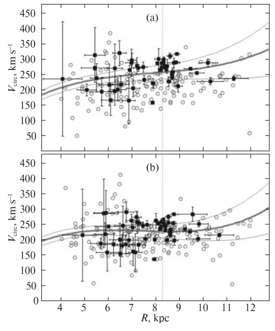
Figure 6 presents two Galactic rotation curves constructed from solutions (9) and (10). When there are only the line-of-sight velocities for PNe, the components of their circular rotation velocities $V_{circ}$ are calculated from the well-known formula

V_{circ}=|R\omega_{0}|+RV_{r}/(R_{0}\sin l\cos b),

(11)

It can be seen from this formula that at small values of $\sin l$ in the denominator these velocities have very large errors. Therefore, when constructing Fig. 6, we excluded the PNe from the cone $|l|<15^{\circ}.$ For PNe with known line-of-sight velocities and proper motions we can calculate their total spatial heliocentric velocities $U,V,$ and $W$ directed along the $x,y,$ and $z$ coordinate axes. For such PNe the rotation velocity $V_{circ}$ is calculated from the relation

V_{circ}=U\sin\theta+(V_{0}+V)\cos\theta,

(12)

where $V_{0}=|R_{0}\omega_{0}|$ and the position angle $\theta$ is defined as $\tan\theta=y/(R_{0}-x)$ .

As can be seen from Fig. 6, the Galactic rotation curve based on the parameters of solution (10) is considerably closer to what is obtained from the analysis of samples with more reliable distances (Zabolotskikh et al. 2002; Bobylev and Bajkova 2011; Reid et al. 2014; Bobylev and Bajkova 2014; Rastorguev et al. 2016). Note that the shape of the rotation curve in the solar neighborhood depends on the Oort constants $A$ and $B,$ because $A+B=\partial V_{circ}/\partial R$ at $R=R_{0}.$ In the case of solution (10), $A+B=-1.4$ km s^-1 kpc^-1 indicates that the Galactic rotation velocity falls near the Sun, which is consistent with the results of the analysis of other data. In contrast, in the case of solution (9), the reverse is true: a large positive value of $A+B$ suggests a dramatic rise of the rotation curve, which is in poor agreement with other data.

Thus, a kinematic analysis of sample II confirmed our previous conclusion about the necessity of reducing the distance scale from Stanghellini and Haywood (2010) approximately by 20%.

The value of $\sigma_{0}=45$ km s^-1 (solution (10)) is the velocity dispersion averaged over all directions. Using the reduced distance scale, we calculated the dispersions of the residual (the differential Galactic rotation and the peculiar motion relative to the local standard of rest were taken into account) velocities for the PNe from the entire sample II (the nebulae of Peimbert’s types IV and V were excluded) as a function of distance: $(\sigma_{U},\sigma_{V},\sigma_{W})=(44,43,49)$ km s^-1 for the sample with $r<6$ kpc (40 nebulae), $(\sigma_{U},\sigma_{V},\sigma_{W})=(44,37,32)$ km s^-1 for the sample with $r<3$ kpc (27 nebulae), or $(\sigma_{U},\sigma_{V},\sigma_{W})=(44,35,33)$ km s^-1 for the sample with $r<2$ kpc (20 nebulae). Note that the closer the sample to the Sun, the more reliable values we obtain. It is interesting to compare these values, for example, with the results of the analysis of 398 white dwarfs from Pauli et al. (2006), where the following velocity dispersions were found: $(\sigma_{U},\sigma_{V},\sigma_{W})=(34,24,18)$ km s^-1 for a sample of thin-disk white dwarfs, $(\sigma_{U},\sigma_{V},\sigma_{W})=(79,36,46)$ km s^-1 for a sample of thick-disk white dwarfs, and $(\sigma_{U},\sigma_{V},\sigma_{W})=(138,95,47)$ km s^-1 for a sample of halo white dwarfs. The velocity $V_{\odot}=27\pm 4$ km s^-1 in solution (10) suggests a slight lag behind the local standard of rest due to an asymmetric drift, which provides evidence for the relative youth of our sample of PNe.

Note that PNe are a set of ‘‘stellar remnants’’ with different absolute ages. Therefore, the distribution of their spatial and kinematic characteristics must correspond by 100% neither to the distribution of young open clusters nor to the properties of older objects. We used the criteria that allowed the bulge and halo objects to be excluded from our samples. Our analysis showed the importance of using Peimbert’s classification; therefore, in our next publications we hope to use more fully the information about the membership of PNe in particular Galactic subsystems.

CONCLUSIONS

Based on published data, we produced a sample of PNe that is complete within 2 kpc of the Sun (sample I). The catalog by Frew (2008), to which we added 29 PNe, served as a basis for this sample. The additions include PNe with measured trigonometric parallaxes and those from the catalog by Stanghellini and Haywood (2010). We estimated the total number of PNe in the Galaxy from this sample to be $N_{tot}=17000\pm 3000$ and determined the vertical disk scale height based on an exponential density distribution to be $h_{1}=197\pm 10$ pc.

The second sample (sample II) includes PNe from the catalog by Stanghellini and Haywood (2010) with minor additions. Based on three density distributions, we found fairly large values of the vertical scale height h from this sample. Here, we used only the PNe with Peimbert’s types I, IIa, IIb, and, in rare cases, III. Thus, we took Galactic thin-disk objects in the overwhelming majority of cases. For example, we found $h_{1}=316\pm 15$ pc for PNe from the range of distances $r<4$ kpc based on an exponential density distribution. Here, we faced the fact that the values of h increase considerably with sample radius. We experimentally found that it is necessary to reduce the distance scale of the catalog by Stanghellini and Haywood (2010) approximately by 20% to obtain acceptable results. In that case, for PNe from the range of distances $r<4$ kpc the vertical scale height is $h_{1}=256\pm 12$ pc, while its values at greater distances are consistent with the results of the analysis of other old Galactic thin-disk objects, more specifically, it does not exceed 300 pc.

We provided sample II with published data on the line-of-sight velocities and proper motions for the central stars of PNe. Based on 226 PNe with reduced distances, we determined the following Galactic rotation parameters: $(U,V,W)_{\odot}=(12,27,7)\pm(3,4,6)$ km s^-1, $\Omega_{0}=\leavevmode\nobreak\ 27.4\pm 2.6$ km s^-1 kpc^-1, $\Omega^{{}^{\prime}}_{0}=-3.47\pm 0.30$ km s^-1 kpc^-2, and $\Omega^{{}^{\prime\prime}}_{0}=\leavevmode\nobreak\ 1.20\pm 0.26$ km s^-1kpc^-3. The Oort constants $A=-14.4\pm 1.2$ km s^-1 kpc^-1 and $B=13.0\pm 2.9$ km s^-1 kpc^-1 correspond to this solution. The linear rotation velocity of the Galaxy at the solar distance is $V_{0}=227\pm 30$ km s^-1 for the adopted $R_{0}=8.3$ kpc. The derived kinematic parameters are in good agreement with those known from the literature. Our analysis of $\Omega^{{}^{\prime}}_{0}$ found confirmed the necessity of reducing the original distance scale of the catalog by Stanghellini and Haywood (2010) by 15–20%.

We are grateful to the referees for their helpful remarks that contributed to an improvement of this paper. This work was supported by the Basic Research Program P–7 of the Presidium of the Russian Academy of Sciences, the ‘‘Transitional and Explosive Processes in Astrophysics’’ Subprogram.

REFERENCES

1. A. Acker, F. Ochsenbein, B. Stenholm, R. Tylenda, J. Marcout, and C. Schohn, in Astronomy from Large Databases II, Proceedings of the 43rd ESO Conference Workshop, Haguenau, September 14–16, 1992, Ed. by A. Heck and F. Murtagh (ESO, 1992), p. 163.

2. D. Alloin, C. Cruz-González, and M. Peimbert, Astrophys. J. 205, 74 (1976).

3. P.R. Amnuel, O.Kh. Guseinov, Kh.I. Novruzova, and Iu.S. Rustamov, Astrophys. Space Sci. 107, 19 (1984).

4. J.N. Bahcall and R.M. Soneira, Astrophys. J. Suppl. Ser. 44, 73 (1980).

5. A.T. Bajkova and V.V. Bobylev, Baltic Astron. 24, 43 (2015).

6. G.F. Benedict, B.E. McArthur, R. Napiwotzki, T.E. Harrison, H.C. Harris, E. Nelan, H.E. Bond, R.J. Patterson, and R. Ciardullo, Astron. J. 138, 1969 (2009).

7. V.V. Bobylev and A.T. Bajkova, Astron. Lett. 37, 526 (2011).

8. V.V. Bobylev and A.T. Bajkova, Astron. Lett. 40, 389 (2014).

9. V.V. Bobylev and A.T. Bajkova, Astron. Lett. 42, 1 (2016a).

10. V.V. Bobylev and A.T. Bajkova, Astron. Lett. 42, 182 (2016b).

11. C. Bonatto, L.O. Kerber, E. Bica, and B.X. Santiago, Astron. Astrophys. 446, 121 (2006).

12. J. Bovy, H.-W. Rix, E.F. Schlafly, D.L. Nidever, J.A. Holtzman, M. Shetrone, and T.C. Beers, Astrophys. J. 823, 30 (2016).

13. A.G.A. Brown, A. Vallenari, T. Prusti, J. de Bruijne, F. Mignard, R. Drimmel, et al. (GAIA Collab.), Astron. Astrophys. 595, A2 (2016).

14. A.S.M. Buckner and D. Froebrich, Mon. Not. R. Astron. Soc. 444, 290 (2014).

15. J.H. Cahn, J.B. Kaler, and L. Stanghellini, Astron. Astrophys. Suppl. Ser. 94, 399 (1992).

16. B. Chen, C. Stoughton, J.A. Smith, A. Uomoto, J.R. Pier, B. Yanny, Ź.E. Ivezić, D.G. York, et al., Astrophys. J. 553, 184 (2001).

17. P.S. Conti and W.D. Vacca, Astron. J. 100, 431 (1990).

18. R.L.M. Corradi and H.E. Schwarz, Astron. Astrophys. 293, 871 (1995).

19. A.K. Dambis, A.M. Mel’nik, and A.S. Rastorguev, Astron. Lett. 27, 58 (2001).

20. D.J. Frew and Q.A. Parker, in Planetary Nebulae in our Galaxy and Beyond, Proceedings of the 234th IAU Symposium, Ed. by M.J. Barlow and R.H. Méndez (Cambridge Univ. Press, Cambridge, 2006), p. 49.

21. D.J. Frew, PhD Thesis (Depart. Phys., Macquarie Univ., NSW 2109, Australia, 2008).

22. D.J. Frew, I.S. Bojičić, and Q. A. Parker,Mon. Not. R. Astron. Soc. 431, 2 (2013).

23. S. Gillessen, F. Eisenhauer, T.K. Fritz, H. Bartko, K. Dodds-Eden, O. Pfuhl, T. Ott, and R. Genzel, Astroph. J. 707, L114 (2009).

24. L. Girardi, M.A.T. Groenewegen, E. Hatziminaoglou, and L. da Costa, Astron. Astrophys. 436, 895 (2005).

25. H.C. Harris, C.C. Dahn, B. Canzian, H.H. Guetter, S.K. Leggett, S.E. Levine, C.B. Luginbuh, A.K.B. Monet, et al., Astron. J. 133, 631 (2007).

26. The Hipparcos and Tycho Catalogues, ESA SP–1200 (1997).

27. E. Hog, C. Fabricius, V.V. Makarov, U. Bastian, P. Schwekendiek, A. Wicenec, S. Urban, T. Corbin, and G. Wycoff, Astron. Astrophys. 355, L27 (2000).

28. M. Honma, T. Nagayama, K. Ando, T. Bushimata, Y.K. Choi, T. Handa, T. Hirota, H. Imai, T. Jike, et al., Publ. Astron. Soc. Jpn. 64, 136 (2012).

29. H. Imai, T. Kurayama, M. Honma, and T. Miyaji, Publ. Astron. Soc. Jpn. 65, 28 (2013).

30. K. Ishida and R. Weinberger, Astron. Astrophys. 178, 227 (1987).

31. G.H. Jacoby, Astrophys. J. Suppl. Ser. 42, 1 (1980).

32. M. Jurić, Z. Ivezić, A. Brooks, R.H. Lupton, D. Schlegel, D. Finkbeiner, N. Padmanabhan, N. Bond, et al., Astrophys. J. 673, 864 (2008).

33. G.S. Khromov, Space Sci. Rev. 51, 339 (1989).

34. Yu. V.Milanova and A.F. Kholtygin, Astron. Lett. 35, 518 (2009).

35. M. Moe and O. de Marco, Astrophys. J. 650, 916 (2006).

36. E.A. Olivier, P. Whitelock, and F. Marang, Mon. Not. R. Astron. Soc. 326, 490 (2001).

37. R. Ortiz, Astron. Astrophys. 560, A85 (2013).

38. Q. A. Parker, A. Acker, D.J. Frew, and W.A. Reid, in Planetary Nebulae in our Galaxy and Beyond, Proceedings of the 234th IAU Symposium, Ed. by M. J. Barlow and R.H. Mendez (Cambridge Univ. Press, Cambridge, 2006), p. 1.

39. E.-M. Pauli, R. Napiwotzki, U. Heber, M. Altmann, and M. Odenkirchen, Astron. Astrophys. 447, 173 (2006).

40. M. Peimbert, IAU Symp. 76, 215 (1978).

41. M. Peimbert, Rev. Mex. Astron. Astrofis. 20, 119 (1990).

42. J.P. Phillips, Mon. Not. R. Astron. Soc. 353, 589 (2004).

43. A.E. Piskunov, N.V. Kharchenko, S. Röser, E. Schilbach, and R.-D. Scholz, Astron. Astrophys. 445, 545 (2006).

44. T. Prusti, J.H.J. de Bruijne, A.G.A. Brown, A. Vallenari, C. Babusiaux, C.A.L. Bailer-Jones, U. Bastian, M. Biermann, et al. (GAIA Collab.), Astron. Astrophys. 595, A1 (2016).

45. C. Quireza, H.J. Rocha-Pinto, and W.J. Maciel, Astron. Astrophys. 475, 217 (2007).

46. A.S. Rastorguev, M.V. Zabolotskikh, A.K. Dambis, N. D. Utkin, A.T. Bajkova, and V.V. Bobylev, arXiv: 1603.09124 (2016).

47. M.J. Reid, K.M. Menten, A. Brunthaler, X.W. Zheng, T.M. Dame, Y. Xu, Y. Wu, B. Zhang, et al., Astrophys. J. 783, 130 (2014).

48. H.-W. Rix and J. Bovy, Astron. Astrophys. Rev. 21, 61 (2013).

49. A.C. Robin, C. Reylé, S. Derriére, and S. Picaud, Astron. Astrophys. 409, 523 (2003).

50. I.S. Shklovskii, Astron. Zh. 33, 222 (1956).

51. H. Smith, Mon. Not. R. Astron. Soc. 449, 2980 (2015).

52. L. Stanghellini, R.A. Shaw, and E. Villaver, Astrophys. J. 689, 194 (2008).

53. L. Stanghellini and M. Haywood, Astrophys. J. 714, 1096 (2010).

54. L. Stanghellini, B. Bucciarelli, M.G. Lattanzi, and R. Morbidelli, arXiv: 1609.08840 (2016).

55. D. Tafoya, H. Imai, Y. Gomez, J.M. Torrelles, N.A. Patel, G. Anglada, L.F. Miranda, M. Honma, et al., Publ. Astron. Soc. Jpn. 63, 71 (2011).

56. S. Vennes, R.J. Smith, B.J. Boyle, S.M. Croom, A. Kawka, T. Shanks, L. Miller, and N. Loaring, Mon. Not. R. Astron. Soc. 335, 673 (2002).

57. D.G. York, J. Adelman, J.E. Anderson, S.F. Anderson, J. Annis, N.A. Bahcall, J.A. Bakken, R. Barkhouser, et al., Astrophys. J. 540, 825 (2000).

58. M.V. Zabolotskikh, A.S. Rastorguev, and A.K. Dambis, Astron. Lett. 28, 454 (2002).

59. N. Zacharias, C.T. Finch, T.M. Girard, A. Henden, J.L. Bartlett, D.G. Monet, and M.I. Zacharias, Astron. J. 145, 44 (2013).

60. A.A. Zijlstra and S.R. Pottasch, Astron. Astrophys. 243, 478 (1991).