MOA-2016-BLG-227Lb: A Massive Planet Characterized by Combining Lightcurve Analysis and Keck AO Imaging

Abstract

We report the discovery of a microlensing planet — MOA-2016-BLG-227Lb — with a large planet/host mass ratio of $q\simeq 9\times 10^{-3}$. This event was located near the K2 Campaign 9 field that was observed by a large number of telescopes. As a result, the event was in the microlensing survey area of a number of these telescopes, and this enabled good coverage of the planetary light curve signal. High angular resolution adaptive optics images from the Keck telescope reveal excess flux at the position of the source above the flux of the source star, as indicated by the light curve model. This excess flux could be due to the lens star, but it could also be due to a companion to the source or lens star, or even an unrelated star. We consider all these possibilities in a Bayesian analysis in the context of a standard Galactic model. Our analysis indicates that it is unlikely that a large fraction of the excess flux comes from the lens, unless solar type stars are much more likely to host planets of this mass ratio than lower mass stars. We recommend that a method similar to the one developed in this paper be used for other events with high angular resolution follow-up observations when the follow-up observations are insufficient to measure the lens-source relative proper motion.

1 Introduction

Gravitational microlensing is a powerful method for detecting extrasolar planets (Mao & Paczynski, 1991; Gould & Loeb, 1992; Gaudi, 2012). Compared to other detection techniques, microlensing is sensitive to low-mass planets (Bennett & Rhie, 1996) orbiting beyond the snow line around relatively faint host stars like M dwarfs or brown dwarfs (Bennett et al., 2008; Sumi et al., 2016), which is complementary to other methods.

A difficulty with the microlensing method is the determination of the mass of a lens $M_{L}$ and the distance to the lens system $D_{L}$. If we have an estimate for the angular Einstein radius $\theta_{E}$ and the microlens parallax $\pi_{E}$, the mass is directly determined by

$$M_{L}=\frac{\theta_{\rm E}}{\kappa\pi_{\rm E}}\ ,$$ (1)

where $\kappa=8.144~{}{\rm mas}~{}M_{\odot}^{-1}$ (Gould, 1992; Gaudi et al., 2008; Muraki et al., 2011). When the source distance, $D_{S}\sim 8$ kpc, is known, the distance to the lens is given by

$$D_{L}={{\rm AU}\over\pi_{E}\theta_{E}+\pi_{S}},$$ (2)

where $\pi_{S}\equiv{\rm AU}/D_{S}$. However the microlens parallax can be observed for a fraction of planetary events, while the angular Einstein radius is observed for most planetary events.

One strategy to estimate $M_{L}$ and $D_{L}$ for events in which microlens parallax cannot be detected is to use a Bayesian analysis based on probability distributions from a standard Galactic model (e.g., Beaulieu et al. 2006; Bennett et al. 2014; Koshimoto et al. 2014; Shvartzvald et al. 2014). However, such an analysis must necessarily make an assumption about the probability that stars of a given mass and distance will host a planet. The most common assumption is that all stellar microlens stars are equally likely to host a planet with the properties of the microlens planet in question. It may be that the probability of hosting a planet of the measured mass ratio and separation depends on the host mass or the distance from the Galactic center. But, without mass and distance measurements, these quantities are determined by our Bayesian prior assumptions. As a case in point, Bennett et al. (2014) analyzed MOA-2011-BLG-262 and found a planetary mass host orbited by an Earth-mass “moon” model had almost the same likelihood as a star$+$planet model. But, since we have no precedent for such a rogue planet+moon system, they selected the more conventional star$+$planet system as the favored model. Also, the first discovered microlensing planet, OGLE-2003-BLG-235Lb, was at first thought to be a giant planet orbiting an M dwarf with a mass of $M_{*}\sim 0.36M_{\odot}$ from a Bayesian analysis (Bond et al., 2004). Such a system is predicted to be rare according to the core accretion theory of planet formation (Laughlin et al., 2004; Kennedy & Kenyon, 2008). Follow-up HST images revealed a more massive host star with mass of $M_{*}=0.63^{+0.07}_{-0.09}M_{\odot}$ by detecting excess flux in multiple passbands (Bennett et al., 2006).

When we measure the lens flux with high angular resolution HST or adaptive optics (AO) images (e.g., Bennett et al. 2006, 2007, 2015; Batista et al. 2015), we can then calculate the lens mass $M_{L}$ using a mass-luminosity relation combined with the mass distance relation derived from $\theta_{E}$ measurement. High angular resolution images are needed because microlensed source stars are generally located in dense Galactic bulge fields where there are usually multiple bright main sequence stars per ground-based seeing disk.

Because the size of the angular Einstein radius is $\lower 2.15277pt\hbox{$\;\buildrel<\over{\sim}\;$}1\,$mas, and the lens-source relative proper motion is typically $\mu_{\rm rel}\sim 6\,$mas/yr, it is possible that the lens and source stars will remain unresolved even in high angular resolution images taken within a few years of the microlensing event. In such cases, there will be excess flux above that contributed by the source star and this excess flux must include the lens star flux. Some studies (Batista et al., 2014; Fukui et al., 2015; Koshimoto et al., 2017b), which detected an excess flux, have assumed that this excess flux is dominated by the lens flux, and they have derived the lens mass under this assumption.

With this method, it might seem that no assumptions are required regarding the probability of the microlens stars to host planets, and there would be no biases due to any inadequacies of the Galactic model used. However, Bhattacharya et al. (2017) use HST imaging to show that the excess flux at the position of the MOA-2008-BLG-310 source is not due to the lens star, and Koshimoto et al. (2017a) have developed a Bayesian method to study the possibility of excess flux from stars other than the lens star. Possibilities include unrelated stars, and companions to the source and lens stars. They find that it can be difficult to exclude all these contamination scenarios, especially for events with small angular Einstein radii. In those cases where we cannot exclude the contamination scenarios, we can again use a Bayesian analysis similar to the one described above to estimate the probability distribution of the lens properties. This means that we need to assume prior distributions for stellar binary systems and the stellar luminosity function even when we have detected excess flux in high angular resolution images. In cases where the lens properties are confirmed by a measurement of the lens-source relative proper motion (Bennett et al., 2015; Batista et al., 2015) or microlensing parallax measurements (Gaudi et al., 2008; Beaulieu et al., 2016; Bennett et al., 2016), this contamination can be ruled out. Attempts at lens-source relative proper motion measurements can also confirm contamination (Bhattacharya et al., 2017) in cases where the measured proper motion of the star responsible for the excess flux does not match the microlensing light curve prediction.

In this paper, we report the discovery of the planetary microlensing event MOA-2016-BLG-227. Observations and data reduction are described in Sections 2 and 3. Our modeling results are presented in Section 4. In Section 5, we model the foreground extinction by comparing observed color magnitude diagrams (CMDs) to different extinction laws and compare the results from the different extinction laws. Then, we use the favored extinction law to determine the angular Einstein radius, $\theta_{\rm E}$. In Section 6, we describe our Keck AO observations and photometry, and we determine the excess flux at the position of the source. In Section 7, we describe our Bayesian method to determine the probability that this excess flux is due to lens star and various combinations of other “contaminating” stars. The posterior probabilities for this MOA-2016-BLG-227 planetary microlensing event are presented, and we consider the effect of different planet hosting probability priors. Finally, we discuss and conclude the results of our work in Section 8.

2 Observations

The Microlensing Observations in Astrophysics (MOA; Bond et al. 2001, Sumi et al. 2003) group conducts a high cadence survey towards the Galactic bulge using the 2.2-deg² FOV MOA-cam3 (Sako et al., 2008) CCD camera mounted on the 1.8 m MOA-II telescope at the University of Canterbury Mt. John Observatory in New Zealand. The MOA group alerts about 600 microlensing events per year. Most observations are conducted in a customized MOA-Red filter which is similar to the sum of the standard Cousins $R$-and $I$-band filters. Observations with the MOA $V$ filter (Bessell $V$-band) are taken once every clear night in each MOA field.

The microlensing event MOA-2016-BLG-227 was discovered and announced by the MOA alert system (Bond et al., 2001) at (R.A., Dec.)_J2000 = (18:05:53.70, -27:42:51.43) and $(l,b)=(3.303^{\circ},-3.240^{\circ})$ on 5 May 2016 (HJD${}^{\prime}\equiv$ HJD - 2450000 $\sim$ 7514). This event occurred during the microlensing Campaign 9 of the K2 Mission (K2C9; Henderson et al. 2016) and it was located close to (but not in) the area of sky that was surveyed for the K2C9. This part of the K2 field that was downloaded at 30 minute intervals is known as the “superstamp.” Because this event was so close to the superstamp, several other groups conducting observing campaigns coordinated with the K2C9 observations also observed this event.

The Wise group used the Jay Baum Rich telescope, a Centurion 28 inch telescope (C28) at the Wise Observatory in Israel, which is equipped with a 1 deg² camera. The group monitored the K2C9 superstamp during the campaign with six survey fields that were observed 3–5 times per night with the Astrodon Exo- Planet BB (blue-blocking) filter. Although the MOA-2016-BLG-227 target was just outside the K2C9 superstamp, it was still within the Wise survey footprint.

The event was also observed with the wide-field near infrared (NIR) camera (WFCAM) on the UKIRT 3.8m telescope on Mauna Kea, Hawaii, as part of a NIR microlensing survey in conjunction with the K2C9 (Shvartzvald et al., 2017) survey. The UKIRT survey covered 6 deg², including the entire K2C9 superstamp and extending almost to the Galactic plane, with a cadence of 2–3 observations per night. Observations were taken in $H$-band, with each epoch composed of sixteen 5-second co-added dithered exposures (2 co-adds, 2 jitter points, and $2\times 2$ microsteps).

The Canada France Hawaii Telescope (CFHT), also on Mauna Kea, serendipitously observed the event during the CFHT-K2C9 Microlensing Survey. The CFHT operated a multi-color survey of the K2C9 superstamp using the Megacam Instrument (Boulade et al., 2003). The CFHT observations for the event were conducted through the $g$-, $r$- and $i$-band filters.

The VLT Survey Telescope (VST) is a 2.61m telescope installed at ESO’s Paranal Observatory, and it carried out K2C9 observations as a 99-hours filler program (Arnaboldi et al., 1998; Kuijken et al., 2002). Observations for such a filler program could only be carried out whenever the seeing was worse than 1 arcsec or conditions were non-photometric. The main objective of the microlensing program was to monitor the K2C9 superstamp in an automatized mode to improve the event coverage and to secure color-information in SDSS $r$ and Johnson $V$ passbands. Due to weather conditions, Johnson $V$ images were only taken in the second half of the K2C9 survey, and therefore MOA-2016-BLG-227 is only covered by SDSS $r$. The exact pointing strategy was adjusted to cover the superstamp with 6 pointings and to contain as many microlensing events from earlier seasons as possible. In addition, a two-point dither was obtained to reduce the impact of bad pixels and detector gaps. Consequently, some events, like MOA-2016-BLG-227, received more coverage and have been observed with different CCDs.

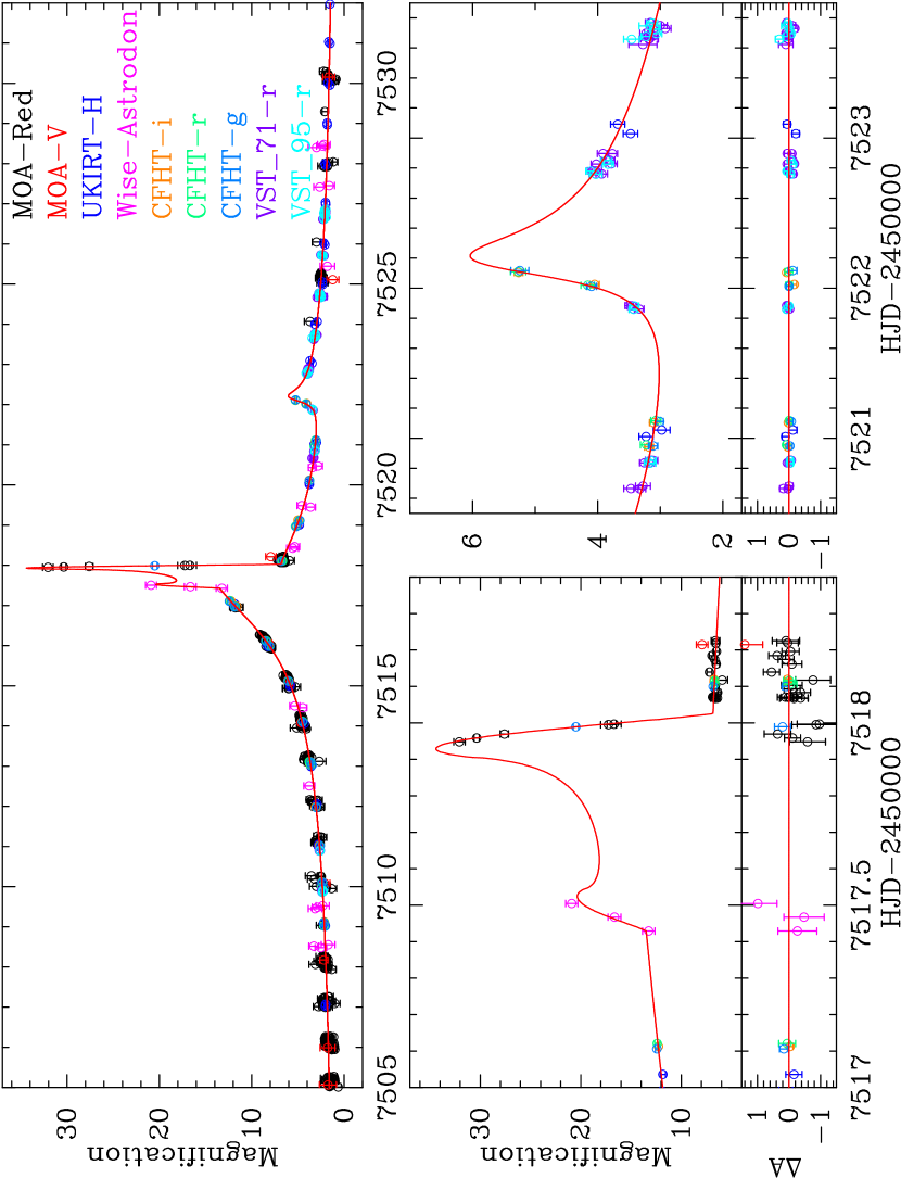
Figure 1: The light curve data for MOA-2016-BLG-227 is plotted with the best-fit model. The top panel shows the whole event, the bottom left and bottom right panels highlight the caustic crossing feature and the second bump due to the cusp approach, respectively. The residuals from the model are shown in the bottom insets of the bottom panels.

Figure 1 shows the observed MOA-2016-BLG-227 light curve. MOA announced the detection of a light curve anomaly for this event on 9 May 2016 (HJD${}^{\prime}=$ HJD $-2450000\sim$ 7518), and identified the anomaly as a planetary signal 4.5 hours after the anomaly alert. Although MOA detected a strong planetary caustic exit, the observing conditions were poor at the MOA observing site both immediately before and after this strong light curve feature. Fortunately, the additional observations from the Wise, UKIRT, CFHT and VST telescopes covered the other important features of the light curve.

3 Data Reduction

Photometry of the MOA, Wise and UKIRT data were conducted using the offline difference image analysis pipeline of Bond et al. (2017) in which stellar images are measured using an analytical PSF model of the form used in the DoPHOT photometry code (Schechter, Mateo, & Saha, 1993).

Differential flux lightcurves of the CFHT data were produced from Elixir calibrated images using a custom difference imaging analysis pipeline based on ISIS version 2.2 (Alard & Lupton, 1998; Alard, 2000) and utilizing an improved interpolation routine (Siverd et al., 2012; Bertin & Arnouts, 1996). Further details of the CFHT data reduction will be presented in a future paper.

Since there is no public VST instrument pipeline, calibration images from ESO’s archive were used and combined. Restrictive bad pixel masks were extracted to prevent inclusion of flatfield pixels with $>1\,\%$ nightly variation or with $>10\,\%$ deviation from the average. The calibrated images were reduced with the difference imaging package DanDIA (Bramich, 2008), which uses a numerical kernel for difference imaging and the routines from the RoboNet pipeline for photometry(Tsapras et al., 2009).

It is known that error bars estimated by crowded field photometry codes can be under or overestimated depending on the specific details of event. The error bars provided by the photometry codes are sufficient to find the best fit models, but they do not allow a proper determination of the microlensing light curve model parameter uncertainties. Therefore, we empirically normalize the error bars for each data set. We used the formula presented in Yee et al. (2012) for normalization, $\sigma_{i}^{\prime}=k\sqrt{\sigma^{2}_{i}+e_{\rm min}^{2}}$ where $\sigma_{i}$ is the original error of the $i$th data point in magnitudes, and the parameters for normalization are $k$ and $e_{\rm min}$. The parameters $k$ and $e_{\rm min}$ are adjusted so that the cumulative $\chi^{2}$ distribution as a function of the number of data points sorted by each magnification of the preliminary best-fit model is a straight line of slope 1.

The dataset used for our analysis and the obtained normalization parameters are summarized in Table MOA-2016-BLG-227Lb: A Massive Planet Characterized by Combining Lightcurve Analysis and Keck AO Imaging.

4 Modeling

The modeling of a binary-lens event requires following parameters: the time of the source closest approach to the lens center of mass, $t_{0}$, the impact parameter, $u_{0}$, of the source trajectory with respect to the center of mass of the lens system, the Einstein radius crossing time $t_{\rm E}=\theta_{\rm E}/\mu_{\rm rel}$, the lens mass ratio, $q\equiv M_{\rm p}/M_{\rm host}$ the separation of the lens masses, $s$, the angle between the trajectory and the binary lens axis, $\alpha$, and the source size $\rho\equiv\theta_{*}/\theta_{\rm E}$. The parameters $u_{0}$, $s$, and $\rho$ are given in units of the Einstein radius, and $M_{\rm host}$ and $M_{\rm p}$ are the masses of the host star and its planetary companion. With these seven parameters, we can calculate the magnification as a function of time $A(t)$. In the crowded stellar fields where most microlensing events are found, most source stars are blended with one or more other stars, so that we cannot determine the source star brightness directly from images where the source is not magnified. Therefore, we add another set of linear parameters for each data set, the source and blend fluxes, $f_{S}$ and $f_{b}$, which are related to the observed flux by $F(t)=f_{S}A(t)+f_{b}$.

When we include the finite source effect, we must consider limb darkening effects. We adopt a linear limb-darkening law with one parameter, $u_{\lambda}$, for each data set. From the intrinsic source color, discussed in Section 5.1, we choose the atmospheric parameters for stars with similar intrinsic color from Bensby et al. (2013). This yields an effective temperature of $T_{\rm eff}\sim 5500$ K, a surface gravity of $\log~{}[g/({\rm cm~{}s^{-2}})]=4.0$, a metallicity of [M/H] = 0.0, and a microturbulence velocity of $\xi=1.0~{}{\rm km~{}s^{-1}}$. We select the limb-darkening coefficients from the ATLAS model by Claret & Bloemen (2011) using these atmospheric parameters. We have $u_{\rm MOA-Red}=0.5585$ for MOA-Red, $u_{V}=0.6822$ for MOA-$V$, $u_{R}=0.6015$ for Wise Astrodon, $u_{H}=0.3170$ for UKIRT $H$, $u_{i}=0.5360$ for CFHT $i$, $u_{r}=0.6257$ for CFHT $r$, VST-71 $r$ and VST-95 $r$, and $u_{g}=0.7565$ for CFHT $g$. We used the mean of the $u_{I}$ and $u_{R}$ values for the limb-darkening coefficients for the MOA-Red passband. Here we adopted the $R$-band limb-darkening coefficient for the Wise Astrodon data. As the Wise Astrodon filter is non-standard, our choice is not perfect. However we note that even if we adopt $u=0$ for the limb darkening coefficient used with the Wise data, our $\chi^{2}$ value changes by only 1.5. The limb-darkening coefficients are also listed in Table MOA-2016-BLG-227Lb: A Massive Planet Characterized by Combining Lightcurve Analysis and Keck AO Imaging.

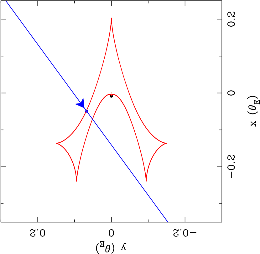
Figure 2: The caustic curve for the best-fit model. The blue arrowed line indicates the source trajectory and the tiny blue circle on the caustic entry indicates the source size.

To find the best-fit model, we conduct a global grid search using the method of Sumi et al. (2016) where we fit the light curves using the Metropolis algorithm (Metropolis et al., 1953), with magnification calculations from the image centered ray-shooting method (Bennett & Rhie, 1996; Bennett, 2010). From this, we find a unique model in which the source crosses the resonant caustic. We show the model light curve in Figure 1, the caustic and the source trajectory in Figure 2 and the best-fit model parameters in Table MOA-2016-BLG-227Lb: A Massive Planet Characterized by Combining Lightcurve Analysis and Keck AO Imaging along with the parameter error bars, which are calculated with a Markov Chain Monte Carlo (MCMC) (Verde et al., 2003).

We also model the light curve including the microlensing parallax effect due to the Earth’s orbital motion (Gould, 1992; Alcock et al., 1995) although this event is unlikely to reveal a significant microlensing parallax signal because of its relatively short timescale. We find that the inclusion of the parallax effect improves the fit by $\Delta\chi^{2}\sim 14$. However, the parts of the lightcurve which contribute to this decrease in $\chi^{2}$ have a scatter similar to the variability of the MOA baseline data, and the best fit microlensing parallax parameter is abnormally large, $\pi_{E}=1.3^{+2.1}_{-0.3}$, yielding a very small lens mass of $M_{L}\sim 0.02M_{\odot}$. Therefore, we conclude that the improvement of the fit by the parallax effect is due to systematic errors in the MOA baseline data.

5 Angular Einstein Radius

Because we have measured the finite source size, $\rho$, to a precision of $\sim 2\,$%, the determination of the angular source star radius $\theta_{*}$ will yield the angular Einstein radius $\theta_{E}=\theta_{*}/\rho$. This, in turn, provides the mass-distance relation, (Bennett, 2008; Gaudi, 2012)

$$M_{L}={c^{2}\over 4G}\theta_{E}^{2}{D_{S}D_{L}\over D_{S}-D_{L}}=0.9823\,M_{\odot}\left({\theta_{E}\over 1\,{\rm mas}}\right)^{2}\left({x\over 1-x}\right)\left({D_{S}\over 8\,{\rm kpc}}\right)\ ,$$ (3)

where $x=D_{L}/D_{S}$. We can empirically derive $\theta_{*}$ from the intrinsic source magnitude and the color (Kervella et al., 2004; Boyajian et al., 2014).

5.1 Calibration

Our fist step is to calibrate the source magnitude to a standard photometric system. We cross referenced stars in the event field between our DoPHOT photometry catalog of stars in the MOA image and the OGLE-III catalog (Szymański et al., 2011) to convert MOA-Red and MOA $V$ into standard magnitudes. Following the procedure presented in Bond et al. (2017), we find the relations

$$I_{\rm OGLE-III}-R_{\rm MOA} =(28.186\pm 0.006)-(0.247\pm 0.005)(V-R)_{\rm MOA}$$ (4)

$$V_{\rm OGLE-III}-V_{\rm MOA} =(28.391\pm 0.004)-(0.123\pm 0.004)(V-R)_{\rm MOA}.$$ (5)

Using these calibration formulae and the result of light curve modeling, we obtain the source star magnitude $I_{S}=19.536\pm 0.019$ and the color $(V-I)_{S}=1.60\pm 0.03$.

We follow a similar procedure to cross referenced stars in our DoPHOT photometry catalog of stars in the UKIRT images to stars in the VVV (Minniti et al., 2010) catalog which is calibrated to the Two Micron All Sky Survey (2MASS) photometric system (Carpenter, 2001), thereby obtaining the relationship between these photometric systems. We use this same VVV catalog to plot CMDs in the next section and for the analysis of the Keck images in Section 6. Using the UKIRT $H$-band source magnitude obtained from the light curve model and the calibration relation, we find $H_{S}=17.806\pm 0.017$. We also measure the colors of the source star: $(V-H)_{S}=3.33\pm 0.03$ and $(I-H)_{S}=1.730\pm 0.017$.

5.2 Extinction and the angular Einstein radius

Next, we correct for extinction following the standard procedure (Yoo et al., 2004; Bennett et al., 2010) using the centroid of red giant clump (RGC) in the CMD as a standard candle.

5.2.1 RGC centroid measurement

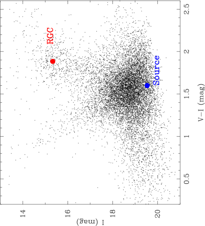
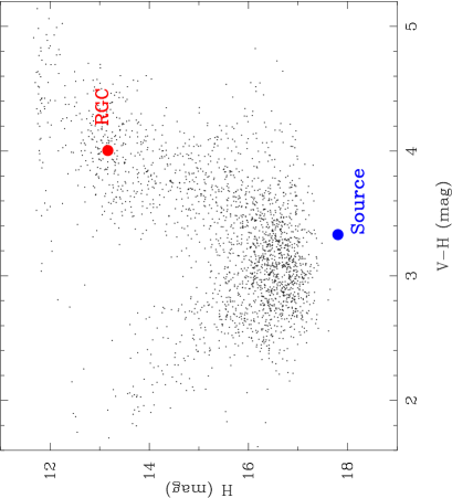
Figure 3: The color magnitude diagrams (CMDs) of stars within $2^{\prime}$ of the source star. The left panel shows $V-I$ vs $I$ for the stars in OGLE-III catalog (Szymański et al., 2011), and the right panel shows $V-H$ vs $H$ using stars from the OGLE-III catalog to the VVV catalog, which is calibrated to the 2MASS magnitude scale. The source star and the mean of red giant clump are shown as the blue and red dots, respectively.

Figure 3 shows the ($V-I$,$I$) and ($V-H$,$H$) CMDs for stars within 2 arcmin of the source star. The $V$ and $I$ magnitudes are taken from the OGLE-III photometry catalog (Szymański et al., 2011), and the VVV (Minniti et al., 2010) catalog to the 2MASS photometry scale for $H$-band magnitudes. To plot the $V-H$ vs $H$ CMD, we cross referenced stars in the VVV catalog to stars in the OGLE-III catalog. For this cross reference, we use only isolated stars that are cross-matched to within 1 arcsec of stars in the OGLE-III catalog to ensure one-to-one matching between the two catalogs. We note that the 1-arcsec limits corresponds to the average seeing in the VVV images. We find the centroids of RGC in the $(V-I,I)$ and $(V-H,H)$ CMDs are $I_{\rm cl}=15.33\pm 0.05$, $(V-I)_{\rm cl}=1.88\pm 0.02$, $(V-H)_{\rm cl}=4.03\pm 0.06$ and $(I-H)_{\rm cl}=2.11\pm 0.03$.

5.2.2 RGC intrinsic magnitude and color

We use $(V-I)_{\rm cl,0}=1.06\pm 0.03$ and $I_{\rm cl,0}=14.36\pm 0.05$ for the intrinsic $V-I$ color and $I$ magnitude of the RGC (Bensby et al., 2013; Nataf et al., 2016) at the Galactic longitude of this event. Following Nataf et al. (2016), we calculate the intrinsic color of $V-H$ and $I-H$ in the photometric system we are using now (i.e., Johnson $V$, Cousins $I$ and 2MASS $H$) by the tool provided by Casagrande & VandenBerg (2014) which is based on a grid of MARCS model atmospheres (Gustafsson et al., 2008). Assuming the stellar atmospheric parameters [Fe/H] = $-0.07\pm 0.10$ (Gonzalez et al., 2013), $\log~{}g=2.3\pm 0.1$ and [$\alpha$/Fe] = $0.20\pm 0.05$ (Hill et al., 2011; Johnson et al., 2014) for the RGC in the event field, we derive $(V-H)_{\rm cl,0}=2.36\pm 0.09$ and $(I-H)_{\rm cl,0}=1.30\pm 0.06$ by adjusting the last atmospheric parameter $T_{\rm eff}$ so that the $(V-I)$ value is in the range of $1.03<(V-I)<1.09$. We summarize the magnitude and colors for the RGC centroid and the source in Table MOA-2016-BLG-227Lb: A Massive Planet Characterized by Combining Lightcurve Analysis and Keck AO Imaging.

5.2.3 Angular Einstein radius

By subtracting the intrinsic RGC color and magnitude values from the measured RGC positions in our CMDs, we find an extinction values of $A_{I,{\rm obs}}=0.98\pm 0.07$, and color excess values of $E(V-I)_{\rm obs}=0.82\pm 0.04$, $E(V-H)_{\rm obs}=1.67\pm 0.11$ and $E(I-H)_{\rm obs}=0.81\pm 0.07$. Following the method of Bennett et al. (2010), we fit these values to the extinction laws of Cardelli et al. (1989), Nishiyama et al. (2009) and Nishiyama et al. (2008) separately and compared the results. We present this analysis in Appendix A. From this comparison of models, we choose the Nishiyama et al. (2008) extinction law, which yields an H-band extinction of $A_{H}=0.19\pm 0.02$ and a source angular radius of $\theta_{*}=0.68\pm 0.02~{}\mu$as. This $\theta_{*}$ value implies an angular Einstein radius of $\theta_{E}=\theta_{*}/\rho=0.227^{+0.006}_{-0.009}$ mas and a lens-source relative proper motion of $\mu_{\rm rel}=\theta_{E}/t_{E}=4.88^{+0.14}_{-0.17}$ mas/yr.

6 Excess Flux from Keck AO Images

On August 13, 2016 (HJD^′ = 7613.85) we observed MOA-2016-BLG-227 using the NIRC2 camera and the laser guide star (LGS) adaptive optics (AO) system mounted on the Keck II telescope at Mauna Kea, Hawaii. Observations were conducted in the $H$-band using the wide-field camera (0.04”/pix). We took four dithered frames with 5 sec exposures and three additional dithered frames with a total integration time of 90 sec (6 co-adds of 15 sec exposures). The first set of these images allows photometric calibration using unsaturated bright stars, and the second set provides the increased photometric sensitivity to provide a high signal-to-noise flux measurement of the target. Standard dark and flat field corrections were applied to the images, and sky subtraction was done using a stacked image from a nearby empty field. Each set of images was then astrometrically aligned and stacked. Finally, we use SExtracor (Bertin & Arnouts, 1996) to extract the Keck source catalog from the stacked images.

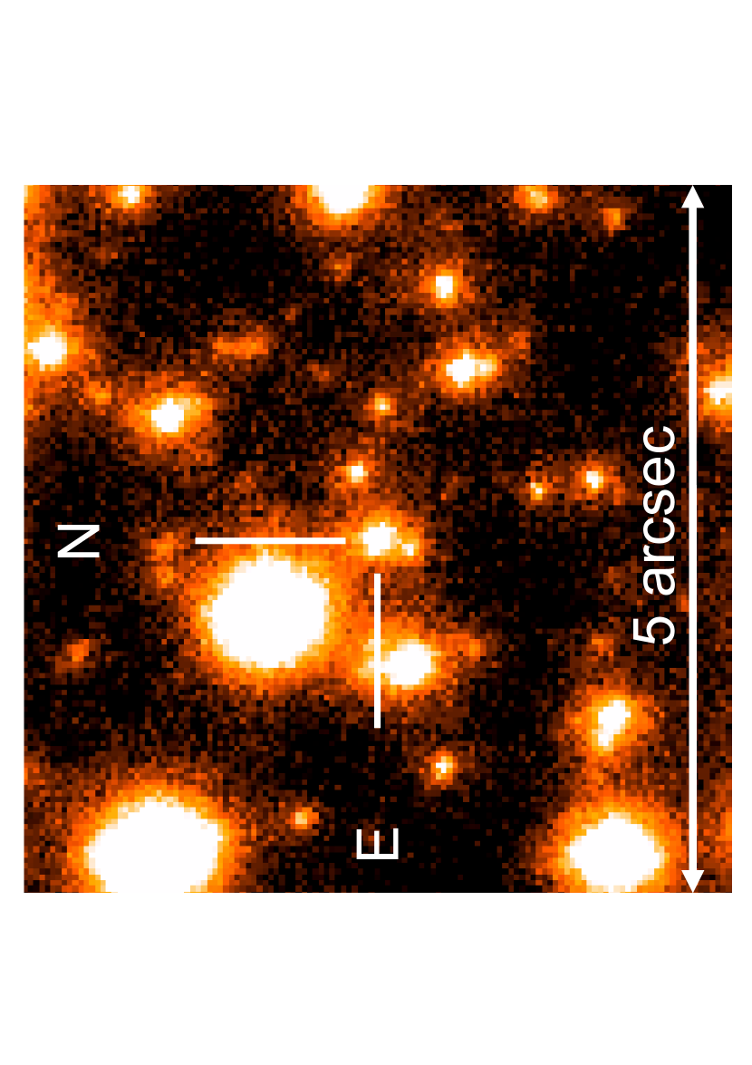
Figure 4: The co-added Keck II AO image of the event field. The target is indicated.

A calibration catalog was extracted using an $H$-band image of the target area taken by the VISTA Variables in the Via Lactea survey (VVV; Minniti et al. 2010) reprocessed following the approach described in Beaulieu et al. (2016). We apply a zero point correction for the Keck source catalog using common VVV and Keck sources. The estimated zero point uncertainty is 0.05. Figure 4 shows the Keck II AO image of the field. It indicates a bright star close to the target. As a result, the dominant photometry error comes from the background flux in the wings of the PSF of the nearby star.

We determine the source coordinates from a MOA difference image of the event while it was highly magnified. We then identify the position of the microlensing target (source+lens) on the Keck image (see Figure 4). The measured brightness of the target is $H_{\rm Keck}=17.63\pm 0.06$. Due to technical problems in the AO system, the stellar images display sparse halo around each object. Thus, the FWHM of the Keck image is 0.184^′′ (measured as the average of isolated bright stars near the target). This sets a limit on our ability to exclude flux contribution from stars unrelated to the source and the lens, as we discuss below.

The light curve analysis of the UKIRT data $H$-band data implies an (extinction uncorrected) $H$-band source magnitude of $H_{S}=17.806\pm 0.017$ (see Section 5.1). Because the Keck observations were taken after the event reached its baseline brightness ($t_{\rm obs,Keck}-t_{0}=5.7~{}t_{E}$), we can extract the excess flux by subtracting the source flux from the target flux. That is, $H_{\rm ex,obs}=H_{S}-2.5\log(F_{\rm Keck}/F_{S}-1)=19.7\pm 0.4$, where $F_{\rm Keck}/F_{S}=10^{-0.4(H_{\rm Keck}-H_{S})}$.

7 Lens Properties through Bayesian Analysis

Koshimoto et al. (2017a) present a systematic Bayesian analysis for the identification of the star or stars producing excess flux at the position of the source seen in high-angular resolution images. This analysis gives us the posterior probability distributions for the lens mass and the distance by combining the results of the light curve modeling and the measured excess flux value. The method is summarized as follows.

1. Determine prior probability distributions for four possibilities for the origin of the excess flux: the lens star, unrelated ambient stars, source companions or lens companions. We denote these fluxes by $F_{L}$, $F_{\rm amb}$, $F_{SC}$ and $F_{LC}$, respectively.

2. Determine all combinations of the flux values for each type of star in the prior distribution that are consistent with the observed excess flux, $F_{\rm excess}=F_{L}+F_{\rm amb}+F_{SC}+F_{LC}$.

The extracted combinations at step 2 corresponds to the posterior probability distributions for the MOA-2016-BLG-227 event.

7.1 Prior probability distributions

Now, we must determine the prior probability distributions of the four types of stars that can contribute to the excess flux at the position of the source. We use all the information we have about this event — except for the value of excess flux — to create our prior probability distributions. This means that we include the FWHM of the Keck images, but not the measured magnitude of the object at the location of the microlensing event. Table MOA-2016-BLG-227Lb: A Massive Planet Characterized by Combining Lightcurve Analysis and Keck AO Imaging shows a summary of our assumptions.

7.1.1 Lens flux prior

For the lens flux prior distribution, we conduct a Bayesian analysis using the observed $t_{E}$ and $\theta_{E}$ values and the Galactic model, which has been used in a number of previous papers (Alcock et al., 1995; Beaulieu et al., 2006) to estimate lens properties for events with no microlensing parallax signal. We use the Galactic model of Han & Gould (1995) for the density and the velocity models and use the mass function presented in the Supplementary Information section of Sumi et al. (2011). Using this result and the mass-luminosity relation presented in Koshimoto et al. (2017a), we obtain the prior distribution for the lens apparent magnitude, $H_{L}$. We adopt the formula for the extinction to the lens, $A_{H,L}=(1-e^{-D_{L}/h_{\rm dust}})/(1-e^{-D_{S}/h_{\rm dust}})~{}A_{H,S}$, following Bennett et al. (2015), where $h_{\rm dust}=(0.1~{}{\rm kpc})/\sin{|b|}$ is the scale length of the dust toward the Galactic bulge, assuming a scale height of $0.1\,$kpc. Note that this Bayesian analysis gives us prior distributions for $M_{L}$, $D_{L}$ and $D_{S}$, in addition to the $H_{L}$ prior distribution, but based on the observed $t_{E}$ and $\theta_{E}$ values. These values are needed for the calculation of the probability distributions below.

7.1.2 Ambient star flux prior

In order to determine the prior probability distribution for the flux of any unrelated ambient stars, we determine the number density of stars in Keck AO images, centered on the target, within a magnitude range selected to have high completeness and divide that number by the area of the image. Then we use the luminosity function of Zoccali et al. (2003) to derive the number density of stars as a function of $H$ magnitude, normalized to this measured number density in the Keck AO image. In this calculation, we correct for the differences in extinction and distance moduli between our field and that of Zoccali et al. (2003), using the distance moduli from Table 3 of Nataf et al. (2013) and extinction values for both fields.

When correcting for the extinction difference, we also consider the difference between the extinction laws used. Zoccali et al. (2003) derived an $A_{H}$ value using the C89 extinction law with $R_{V}=3.1$, whereas our preferred N08 extinction law implies a significantly different $A_{H}$ value. To correct for this difference, we calculate the $A_{H}$ value towards their field using the N08 extinction law fit to the RGC centroid in the OGLE-III CMD and the $R_{JKVI}$ value from Table 3 of Nataf et al. (2013) for their field. The $A_{H}$ value we derived here is $A_{H}=0.122$, which is different from the value of $A_{H}=0.265$ used by Zoccali et al. (2003). Therefore, we convert their extinction corrected $H$-band luminosity function to a luminosity function with our preferred extinction model by adding $\Delta A_{H}=0.265-0.122=0.142$ to their extinction corrected magnitudes, and then add the extinction appropriate for our field, $A_{H}=0.19$.

We assume that stars can be resolved only if they are separated from the source by $\geq 0.8\,{\rm FWHM}=148\,$mas. Under this assumption, the expected number of ambient stars within the circle is derived by multiplying the area of this unresolvable region by the total number density derived above. We determine the number of stars following the Poisson distribution with the mean value of the expected number of stars. We use the corrected luminosity function to determine the magnitude of each star.

7.1.3 Source and lens companion flux priors

We calculate the source and lens companion flux priors with the stellar binary distribution described in Koshimoto et al. (2017a). The binary distribution is based on the summary in a review paper (Duchêne & Kraus, 2013), which provides distributions of the stellar multiplicity fraction, and mass ratio and semi-major axis distributions.

For the flux of source companions, we calculate the source mass $M_{SC}=q_{SC}M_{S}$ and then convert that into a source companion magnitude, $H_{SC}$, using a mass-luminosity relation. The mass ratio $q_{SC}$ is derived from the binary distribution. We derive the source mass, $M_{S},$ from the combination of $H_{S}$, $D_{S}$ and using the mass-luminosity relation. Similarly, we calculate the lens companions magnitude, $H_{LC}$, from $M_{LC}=q_{LC}M_{L}$, where the lens mass $M_{L}$ comes from the same distribution that was used to obtain the lens flux probability distribution.

We consider companions to the lens or source located in the same unresolvable regions in the vicinity of the source, just as in the case of ambient stars. Stellar companions have a separation distribution that is much closer to logarithmic than the uniform distribution expected for ambient stars. As a result, we must now exclude companions that are too close to the source and lens as well as companions that are so widely separated that they will be resolved. Companions that are too close to the source could be magnified themselves, and companions that are too close to the lens could serve as an additional lens star. Such a constraint would have no effect on the ambient star probablity, because the probability of an ambient star very close to the source or lens is much smaller than that of a stellar companion. Following Batista et al. (2014), we adopt $\theta_{E}/4$ as the close limit for source companions and $w_{LC}<u_{0}$ as the close limit for lens companions, where $w_{LC}=4q_{LC}/(s_{LC}-s_{LC}^{-1})^{2}$ (Chung et al., 2005) and $q_{LC}$ and $s_{LC}$ and are the stellar binary lens mass ratio and separation, respectively. We take 0.8 FWHM as the maximum unresolvable radius.

We also consider triple and quadruple systems when estimating the effect of companions to the source and lens, following Koshimoto et al. (2017a), but we find no significant difference from the case of only considering binary systems. We therefore do not include triple and quadruple systems in this analysis, for simplicity.

7.1.4 Excess flux prior

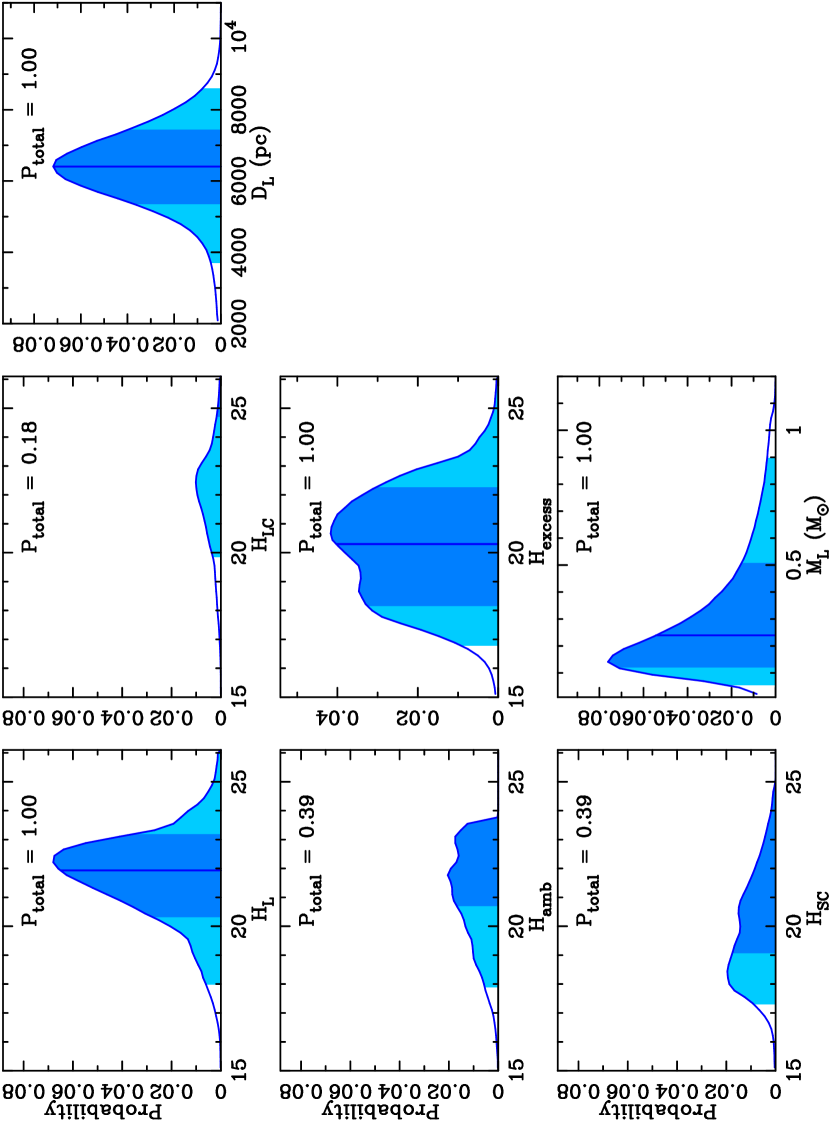
Figure 5: The prior probability distributions using the assumptions in Table MOA-2016-BLG-227Lb: A Massive Planet Characterized by Combining Lightcurve Analysis and Keck AO Imaging and light curve model constraints, as well as the seeing of the Keck AO image, but not the target flux. We assume that the planet hosting probability does not depend on the stellar mass. The borders between dark and light shaded regions indicate the $1\sigma$ limits and the borders between light shaded and white regions indicate $2\sigma$ limits. The $P_{\rm total}$ value in each panel is the probability that the object exists. The panels with $P_{\rm total}<1$ indicate the probability that the companion or ambient star actually exists, and some of these do not have the borders of the $1\sigma$/$2\sigma$ limit within the plotted region.

Figure 5 shows the prior probability distributions we derived following the procedure described above to calculate flux of each type of stars. In addition to the magnitude of the four types of stars that might contribute to the excess flux, we show the prior distributions for the total excess flux, $H_{\rm excess}$, the lens mass, $M_{L}$, and the distance to the lens $D_{L}$. Some of the panels in this figure have total probabilities $P_{\rm total}<1$. This is because many stars do not have binary companions and there is a large probability of no measurable flux from an ambient star. The $H_{\rm excess}$ prior indicates a high probability at the observed magnitude of $H_{\rm ex,obs}=19.7\pm 0.4$. The three panels for individual stars, $H_{L}$, $H_{\rm amb}$ and $H_{SC}$ show similar probabilities at the observed excess flux value. This indicates that it will be difficult to claim that all of the excess comes from the lens itself.

7.2 Posterior probability distributions

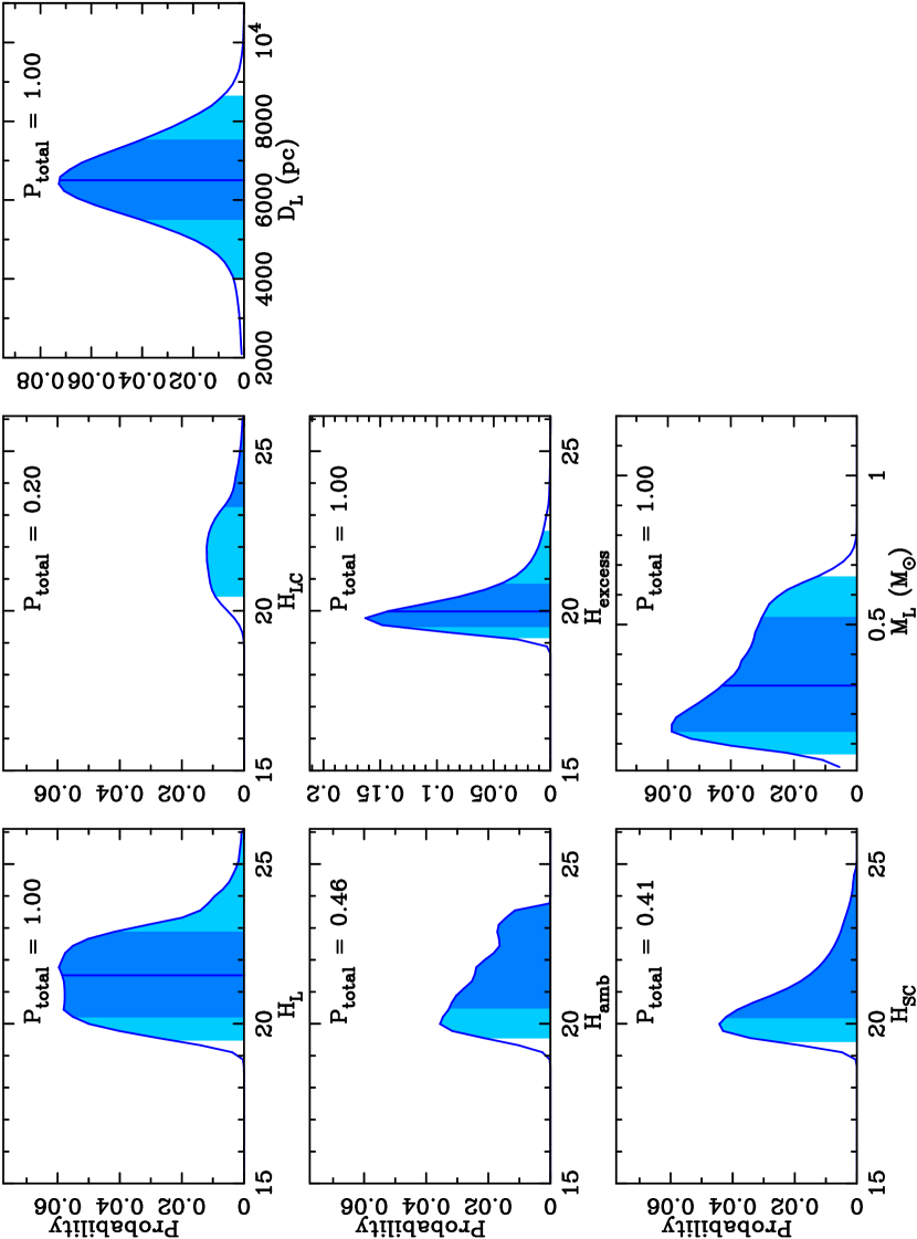
Figure 6: The posterior probability distributions generated by extracting combinations which have consistent excess flux values with $H_{\rm ex,obs}=19.7\pm 0.4$ (in flux unit) from the prior probability distributions in Figure 5.

We generate the posterior probability distributions shown in Figure 6 by extracting combinations of parameters which have values of $H_{\rm excess}$ consistent with the measured value of $H_{\rm ex,obs}=19.7\pm 0.4$ using a Gaussian distribution in fluxes (not magnitudes). The probability that $H_{L}\leq 20$ is almost same as the probability for $H_{\rm SC}\leq 20$ and slightly higher, but competitive with the probability that $H_{\rm amb}\leq 20$, which results in very loose constraints on $H_{L}$ and $M_{L}$. This result is consistent with our expectation as discussed in Section 7.1.4.

The third to sixth columns of Table MOA-2016-BLG-227Lb: A Massive Planet Characterized by Combining Lightcurve Analysis and Keck AO Imaging shows the median, the 1 $\sigma$ error bars, and the 2 $\sigma$ range for $H_{L}$, $M_{L}$ and $D_{L}$ for both the prior and posterior distributions. This same table also shows the values of the planet mass $M_{\rm p}$, the projected separation $a_{\perp}$ and the three-dimensional star-planet separation $a_{3d}$ calculated from the probability distributions, where $a_{3d}$ is statistically estimated assuming a uniform orientation for the detected planets. In the bottom three rows, we present the probabilities that the fraction of the excess flux due to the lens, $f_{L}$ is larger than 0.1, 0.5 and 0.9, which correspond to magnitude difference between the lens and the total flux excess of 2.5 mag, 0.75 mag and 0.11 mag, respectively.

The posterior distributions for the lens system properties are remarkably similar to the prior distributions. When we compare the $1\sigma$ ranges of the prior and posterior distributions, we see that the lens system is most likely to be composed an M or K dwarf star host and a gas-giant planet. However the prior and posterior distributions differ from each other when we consider the $2\sigma$ ranges and the tails of the distributions. The possibility of a G dwarf host star is ruled out by the posterior distribution while the host star can be a G dwarf according to the prior distribution. This implies that the host star is likely to be an M or K dwarf.

7.3 Comparison of different planetary host priors

One assumption that we have made implicitly is that the properties of the lens star do not depend on the fact that we have detected a planet orbiting the star. This assumption could be false. Perhaps more massive stars are more likely to host planets of the measured mass ratio, or perhaps disk stars are more likely to host planets than bulge stars. The microlensing method can be used to address these questions, but we must be careful not to assume the answer to them.

We have assumed that this detection of the planetary signal does not bias any other property of the lens star, such as its mass or distance. If there was a strong dependence of the planet hosting probability at the measured mass ratio of $9.3^{+0.2}_{-0.1}\times 10^{-3}$, then this implicit prior could lead to incorrect conclusions. Some theoretical papers based on core-accretion (Laughlin et al., 2004; Kennedy & Kenyon, 2008) and analyses of exoplanets found by radial velocities (Johnson et al., 2010) have argued that gas giants are less frequently orbiting low-mass stars, however, the difference disappears when the planets are classified by their mass ratio, $q$, instead of their mass. Nevertheless, since the host mass dependence of the planet hosting probability is not well measured, we investigate how our results depend on the choice of this prior.

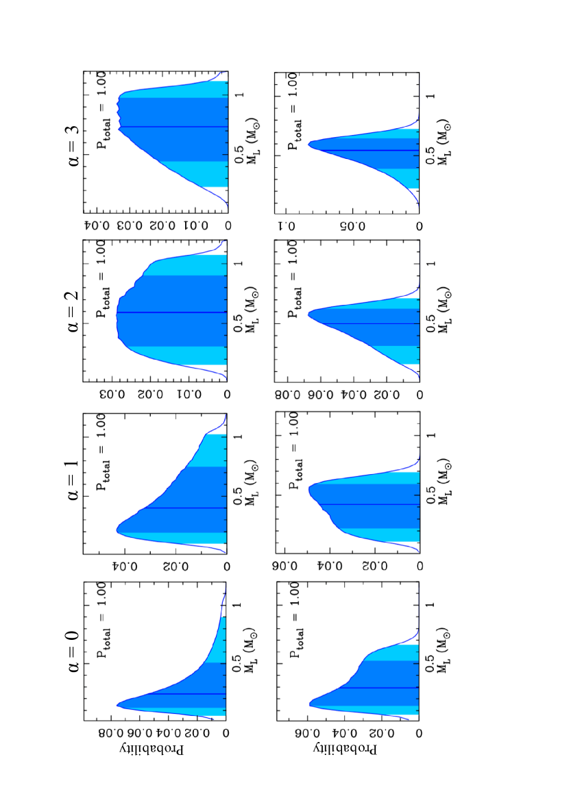
Figure 7: The prior (top) and posterior (bottom) probability distributions of the lens mass $M_{L}$ using different priors for the planet hosting probability, which is assumed to follow a power law, $P_{\rm host}\propto M^{\alpha}$. The $\alpha=0$ plots are repeated from Figures 5 and 6.

We consider a series of prior distributions where the planet hosting probability follows a power law of the form $P_{\rm host}\propto M^{\alpha}$, and we conduct a series of Bayesian analyses with $\alpha=1$, $\alpha=2$ and $\alpha=3$ in addition to the calculation with $\alpha=0$, presented above. Figure 7 shows both the prior and posterior probability distributions for the lens mass, $M_{L}$, with these different values of $\alpha$. The lens property values for each posterior distribution are shown in Table MOA-2016-BLG-227Lb: A Massive Planet Characterized by Combining Lightcurve Analysis and Keck AO Imaging. The median of expected lens flux approaches the measured excess flux as $\alpha$ increases (i.e., the power law becomes steeper), and consequently the median of the lens mass also increases and the parameter uncertainties decrease. Thus, larger $\alpha$ values imply that more of the excess flux is likely to come from the lens. Nevertheless, our basic conclusion that the host is a M or K-dwarf hosting a gas giant planet remains for all of the $1\leq\alpha\leq 3$ priors.

8 Discussion and Conclusion

We have analyzed the planetary microlensing event MOA-2016-BLG-227 which was discovered next to the field observed by the microlensing campaign (Campaign 9) of the K2 Mission. The event and planetary signal were discovered by the MOA collaboration and a significant portion of the planet signal was covered by the data from the Wise, UKIRT, CFHT and VST surveys, which observed the event as part of the K2C9 program. Analysis of these data yields a unique microlensing light curve solution with a relatively large planetary mass-ratio of $q=9.28^{+0.20}_{-0.11}\times 10^{-3}$. We considered several different extinction laws and decided that the N08 (Nishiyama et al., 2008) law was the best fit to our data, although our results would not change significantly with a different law. With this extinction law, we derive an angular Einstein radius of $\theta_{E}=0.227^{+0.006}_{-0.009}\,$mas, which yields the mass-distance relation given in Equation 3. We detected excess flux at the location of the source in a Keck AO image, and we performed a Bayesian analysis to estimate the relative probability of different sources of this excess flux, such as the lens, an ambient star, or a companion to the host or source. Our analysis excludes the possibility that the host star is a G-dwarf, leading us to a conclusion that the planet MOA-2016-BLG-227Lb is a super-Jupiter mass planet orbiting an M or K-dwarf star likely located in the Galactic bulge. Such systems are predicted to be rare by the core accretion theory of planet formation. It is also thought that such a planet orbiting a white dwarf host at $a_{3d}\sim 2$ AU is unlikely (Batista et al., 2011).

If the planet frequency does not depend on the host star mass or distance, our Bayesian analysis indicates the system consists of a host star with mass of $M_{L}=0.29^{+0.23}_{-0.15}M_{\odot}$ orbited by a planet with mass of $M_{\rm p}=2.8^{+2.2}_{-1.5}M_{\rm Jup}$ with a three-dimensional star-planet separation of $a_{3d}=1.67^{+0.94}_{-0.35}$ AU. The system is located at $D_{L}=6.5\pm 1.0\,$kpc from the Sun. We also considered different priors for the planet hosting probability as a function of host star mass. We consider planet hosting prior probabilities that scale as $P_{\rm host}\propto M^{\alpha}$ with $\alpha=1,2,3$, in addition to the $\alpha=0$ prior that we use for our main results. As $\alpha$ increases, the median value of the lens mass also increases and the probability for the lens to be responsible for the excess $H$-band flux increases, as well. Johnson et al. (2010) found a linear (i.e., $\alpha=1$) relationship between host mass and planet occurrence from 0.5 $M_{\odot}$ to 2.0 $M_{\odot}$ for giant planets within $\sim 2$AU around host stars discovered by the radial velocity (RV) method. However, this analysis used a fixed minimum mass instead of a fixed mass ratio, and it does not appear that Johnson et al. (2010) did a detailed calculation of their detection efficiencies. Another result using RV planet data by Montet et al. (2014) gives $\alpha=0.8^{+1.1}_{-0.9}$, using a sample more similar to the microlensing planets, i.e., gas giants orbiting at $0<a<20$ AU around M-dwarf stars. However, our basic conclusion that the MOA-2016-BLG-227L host star is an M or K-dwarf with a gas-giant planet located in the Galactic bulge would not change with a different $\alpha$ value, as indicated in Figure 7 and Table MOA-2016-BLG-227Lb: A Massive Planet Characterized by Combining Lightcurve Analysis and Keck AO Imaging.

The probability that more than 90% of the excess flux seen in the Keck AO images comes from the lens is still 24.0% even assuming $\alpha=0$. This is significant enough that we cannot ignore the possibility that most of the excess flux comes from the lens star. One approach for obtaining further constraints is to get the color of the excess flux. If the excess flux is not from the lens, the derived lens mass and distance with $H_{\rm excess}$ may be inconsistent with the value derived using the excess flux in a different pass band, if we assume that all of the excess flux comes from the lens. However, such a measurement could also yield ambiguous results. Another, more definitive, approach is to observe this event in the future when we can expect to detect the lens-source separation through precise PSF modeling with high resolution space-based data (Bennett et al., 2007, 2015) or direct resolution with AO imaging (Batista et al., 2015). The lens-source relative proper motion value of $\mu_{\rm rel}=4.88^{+0.14}_{-0.17}\,$mas/yr indicates that we can expect to be able to resolve the lens, if it provides a large fraction of the excess flux in $\sim 2022$ using HST (Bhattacharya et al., 2017) and in 2026 using Keck AO (Batista et al., 2015). Observations by the James Webb Space Telescope (Gardner et al., 2006), the Giant Magellan Telescope (Johns et al., 2012), the Thirty Meter Telescope (Nelson & Sanders, 2008) and the Extremely Large Telescope (Gilmozzi & Spyromilio, 2007) could detect the lens-source relative proper motion much sooner. If the separation of the excess flux from the source is different from the prediction of the microlensing model in these future high angular resolution observations, it would indicates that the lens is not the main cause of the excess flux, implying a lower mass planetary host star.

Work by N.K. is supported by JSPS KAKENHI Grant Number JP15J01676. The MOA project is supported by grants JSPS25103508 and 23340064. D.P.B., A.B., and D.S.  were supported by NASA through grants NNX13AF64G, NNX16AC71G, and NNX16AN59G. Work by Y.S. and C.B.H. was supported by an appointment to the NASA Postdoctoral Program at the Jet Propulsion Laboratory, California Institute of Technology, administered by Universities Space Research Association through a contract with NASA. N.J.R. is a Royal Society of New Zealand Rutherford Discovery Fellow. Work by C.R. was supported by an appointment to the NASA Postdoctoral Program at the Goddard Space Flight Center, administered by USRA through a contract with NASA. Work by S.C.N. was supported by NExScI. A.C. acknowledges financial support from Université Pierre et Marie Curie under grants Émergence@Sorbonne Universités 2016 and Émergence-UPMC 2012. This work was supported by a NASA Keck PI Data Award, administered by the NASA Exoplanet Science Institute. Data presented herein were obtained at the W. M. Keck Observatory from telescope time allocated to the National Aeronautics and Space Administration through the agency’s scientific partnership with the California Institute of Technology and the University of California. The Observatory was made possible by the generous financial support of the W. M. Keck Foundation. The authors wish to recognize and acknowledge the very significant cultural role and reverence that the summit of Mauna Kea has always had within the indigenous Hawaiian community. We are most fortunate to have the opportunity to conduct observations from this mountain. The United Kingdom Infrared Telescope (UKIRT) is supported by NASA and operated under an agreement among the University of Hawaii, the University of Arizona, and Lockheed Martin Advanced Technology Center; operations are enabled through the cooperation of the Joint Astronomy Centre of the Science and Technology Facilities Council of the U.K. We acknowledge the support from NASA HQ for the UKIRT observations in connection with $K2$C9. This research uses data obtained through the Telescope Access Program (TAP), which has been funded by the National Astronomical Observatories of China, the Chinese Academy of Sciences (the Strategic Priority Research Program “The Emergence of Cosmological Structures” Grant No. XDB09000000), and the Special Fund for Astronomy from the Ministry of Finance. This work is partly based on observations obtained with MegaPrime/MegaCam, a joint project of CFHT and CEA/DAPNIA, at the Canada-France-Hawaii Telescope (CFHT) which is operated by the National Research Council (NRC) of Canada, the Institut National des Science de l’Univers of the Centre National de la Recherche Scientifique (CNRS) of France, and the University of Hawaii. This work was performed in part under contract with the California Institute of Technology (Caltech)/Jet Propulsion Laboratory (JPL) funded by NASA through the Sagan Fellowship Program executed by the NASA Exoplanet Science Institute. Work by MTP and BSG was supported by NASA grant NNX16AC62G. This work was partly supported by the National Science Foundation of China (Grant No. 11333003, 11390372 to SM). Based on observations made with ESO Telescopes at the La Silla Paranal Observatory under programme ID 097.C-0261.

Appendix A Comparison of Different Extinction Laws

In Section 5.2, we obtained the observed extinction value, $A_{I,{\rm obs}}=0.98\pm 0.07$, and color excess values of $E(V-I)_{\rm obs}=0.82\pm 0.04$, $E(V-H)_{\rm obs}=1.67\pm 0.11$ and $E(I-H)_{\rm obs}=0.81\pm 0.07$. Then, we fit these values to the extinction laws of Cardelli et al. (1989), Nishiyama et al. (2009) and Nishiyama et al. (2008) separately and compared the results. This was motivated by the fact that Nataf et al. (2016) reported a clear difference of their extinction law towards the Galactic bulge from the standard law of Cardelli et al. (1989). Hereafter, we refer to these papers as C89, N09 and N08, respectively. Note that the four observed extinction parameters (1 extinction and 3 color excess) are not independent. They can be derived from the three independent extinction values: $A_{I,{\rm obs}}$, $A_{V,{\rm obs}}$ and $A_{H,{\rm obs}}$.

The C89 law is given by equations (1) - (3b) in their paper, and $A_{V}$ and $R_{V}$ serve as the parameters of their model.

Unlike C89, N09 does not provide a complete extinction model. They provide only ratios of extinctions for wavelengths longer than the $J$-band. So, we need additional information relating $A_{V}$ or $A_{I}$ and $A_{J}$, $A_{H}$ or $A_{K}$ in order to calculate the values that we need for this paper: $A_{I}$, $A_{V}$ and $A_{H}$. Therefore we used the $R_{JKVI}\equiv E(J-K_{s})/E(V-I)$ values from Nataf et al. (2013) in addition to the N09 extinction law. The $R_{JKVI}$ value at the nearest grid point to the MOA-2016-BLG-227 event in Table 3 of Nataf et al. (2013) is 0.3089. However the quality flag for this value is 1, which indicates an unreliable measurement, so we use a conservative uncertainty of $R_{JKVI}=0.31\pm 0.03$. We adjust $A_{I}$ and $E(V-I)$ to minimize the $\chi^{2}$ value between the observed $A_{I,\rm obs}$, $E(V-I)_{\rm obs}$, $E(V-H)_{\rm obs}$, and $E(I-H)_{\rm obs}$ values and those values derived using the ratio $A_{H,{\rm 2MASS}}/E(J-K_{s})_{\rm 2MASS}=0.89$ from N09, in conjunction with the $R_{JKVI}$ value from Nataf et al. (2013). We explicitly use the _2MASS subscript because N09 provides their result also in the IRSF/SIRIUS photometric system (Nagashima et al., 1999; Nagayama et al., 2003). Note that we calculate this $A_{H}/E(J-K_{s})$ value using their result for the field S+ ($0^{\circ}<l<3^{\circ},-1^{\circ}<b<0^{\circ}$), which is nearest of their fields to the MOA-2016-BLG-227 event position.

N08 also provide the ratio of extinctions towards the Galactic bulge ($l\sim 0^{\circ},b\sim-2^{\circ}$). They find $A_{J}/A_{V}=0.183\pm 0.015$, $A_{H}/A_{V}=0.103\pm 0.008$ and $A_{K_{s}}/A_{V}=0.064\pm 0.005$. (These values are slightly different from the original values given by N08 because the values used in N08 were in the OGLE II and IRSF/SIRIUS photometric systems, so we converted them into the standard systems that we use here.) These values are well fit by a single power law, $A_{\lambda}/A_{V}\propto\lambda^{-2}$. Nevertheless, we use the ratios themselves, instead of the single power law, because N08 does not test that their power law accurately reproduces $A_{I}/A_{V}$, which we have now. As in the case of N09, we keep these ratios fixed, and adjust $A_{I}$ and $E(V-I)$ to minimize the $\chi^{2}$ between these relations and the observed $A_{I,\rm obs}$, $E(V-I)_{\rm obs}$, $E(V-H)_{\rm obs}$, and $E(I-H)_{\rm obs}$ values. Notice that N08 had $V$-band data and it was not necessary to use the $R_{JKVI}$ as a constraint. Therefore we used the $R_{JKVI}$ value as the additional observed data instead here in addition to $A_{I,{\rm obs}}$, $A_{V,{\rm obs}}$ and $A_{H,{\rm obs}}$ to increase number of degrees of freedom (dof).

Table MOA-2016-BLG-227Lb: A Massive Planet Characterized by Combining Lightcurve Analysis and Keck AO Imaging shows the results of fitting our extinction measurements to these three different extinction laws. This table also shows the angular source radius calculated from the extinction–corrected source magnitudes and colors using formulae from the analysis of Boyajian et al. (2014). We determine $\theta_{*,IH}$ using Equations (1)-(2) and Table 1 of Boyajian et al. (2014), but the other relations were provided by private communications from Boyajian with a special analysis restricted to stellar colors that are relevant for the Galactic bulge sources observed in microlensing events. We use Equation (4) of Fukui et al. (2015) to determine $\theta_{*,VI}$, and we use Equation (4) of Bennett et al. (2015) to determine $\theta_{*,VH}$. Those formulae are

$$\log~{}[2\theta_{*,VI}/(1{\rm mas})] =0.5014+0.4197(V-I)_{S,0}-0.2I_{S,0},$$ (A1)

$$\log~{}[2\theta_{*,VH}/(1{\rm mas})] =0.5367+0.0727(V-H)_{S,0}-0.2H_{S,0},$$ (A2)

$$\log~{}[2\theta_{*,IH}/(1{\rm mas})] =0.5303+0.3660(I-H)_{S,0}-0.2I_{S,0}.$$ (A3)

If we compare the $\chi^{2}$ value for each model fit in Table MOA-2016-BLG-227Lb: A Massive Planet Characterized by Combining Lightcurve Analysis and Keck AO Imaging, we see that the $\chi^{2}/{\rm dof}$ for the N09 and N08 laws are smaller than the value from the C89 extinction law, although the C89 is not disfavored by a statistically significant amount. (The $p$-value of $\chi^{2}=2.39$ for ${\rm dof}=1$ is still $\sim$0.12.) Note that a contribution of $0.96$ to the total value of $\chi^{2}=1.19$ arises from fitting the $R_{JKVI}$ value to the N08 extinction law. So, the remaining contribution of 0.23 to $\chi^{2}$ arises from fitting the N08 model to our measurements of the RGC centroids. This indicates that the extinction law of N08 agrees with our measurement of the red clump centroids very well, but not quite so well with the $R_{JKVI}$ value, which comes from Nataf et al. (2013).

From the point of view of consistency between the three $\theta_{*}$ values, the standard deviation of the three values (SD${}_{\theta_{*}}$ in the table) is smallest using the N08 extinction laws. The N08 extinction law also yields the smallest error bars for $A_{H}$ and $\theta_{*,VH}$.

Based on this analysis, we have decided to use the results from the N08 extinction laws in our analysis. We use $\theta_{*,VH}$ for the final angular source radius which is $\theta_{*}=0.68\pm 0.02~{}\mu$as. We show the source magnitudes and colors corrected for extinction using the N08 extinction laws in Table MOA-2016-BLG-227Lb: A Massive Planet Characterized by Combining Lightcurve Analysis and Keck AO Imaging.

References

- Alard (2000) Alard, C. 2000, A&AS, 144, 363
- Alard & Lupton (1998) Alard, C., & Lupton, R. H. 1998, ApJ, 503, 325
- Alcock et al. (1995) Alcock, C., Allsman, R. A., Alves, D., et al. 1995, ApJ, 454, L125
- Arnaboldi et al. (1998) Arnaboldi, M., Capaccioli, M., Mancini, D., et al. 1998, The Messenger, 93, 30
- Batista et al. (2011) Batista, V., Gould, A., Dieters, S., et al. 2011, A&A, 529, A102
- Batista et al. (2014) Batista, V., Beaulieu, J.-P., Gould, A., et al. 2014, ApJ, 780, 54
- Batista et al. (2015) Batista, V., Beaulieu, J.-P., Bennett, D. P., et al. 2015, ApJ, 808, 170
- Beaulieu et al. (2016) Beaulieu, J.-P., Bennett, D. P., Batista, V., et al. 2016, ApJ, 824, 83
- Beaulieu et al. (2006) Beaulieu, J.-P., Bennett, D. P., Fouqué, P., et al. 2006, Nature, 439, 437
- Bennett (2008) Bennett, D.P, 2008, in Exoplanets, Edited by John Mason. Berlin: Springer. ISBN: 978-3-540-74007-0, (arXiv:0902.1761)
- Bennett (2010) Bennett, D. P. 2010, ApJ, 716, 1408
- Bennett et al. (2006) Bennett, D. P., Anderson, J., Bond, I. A., Udalski, A., & Gould, A. 2006, ApJ, 647, L171
- Bennett et al. (2007) Bennett, D.P., Anderson, J., & Gaudi, B.S. 2007, ApJ, 660, 781
- Bennett et al. (2014) Bennett, D. P., Batista, V., Bond, I. A., et al. 2014, ApJ, 785, 155
- Bennett et al. (2015) Bennett, D. P., Bhattacharya, A., Anderson, J., et al. 2015, ApJ, 808, 169
- Bennett et al. (2008) Bennett, D. P., Bond, I. A., Udalski, A., et al. 2008, ApJ, 684, 663
- Bennett & Rhie (1996) Bennett, D. P., & Rhie, S. H. 1996, ApJ, 472, 660
- Bennett et al. (2010) Bennett, D. P., Rhie, S. H., Nikolaev, S., et al. 2010, ApJ, 713, 837
- Bennett et al. (2016) Bennett, D.P., Rhie, S.H., Udalski, A., et al. 2016, AJ, 152, 125
- Bensby et al. (2013) Bensby, T., Yee, J. C., Feltzing, S., et al. 2013, A&A, 549, A147
- Bertin & Arnouts (1996) Bertin, E., & Arnouts, S. 1996, A&AS, 117, 393
- Bhattacharya et al. (2017) Bhattacharya, A., Bennett, D. P., Anderson, J., 2017, AJ, submitted (arXiv:1703.06947)
- Bond et al. (2001) Bond, I. A., Abe, F., Dodd, R. J., et al. 2001, MNRAS, 327, 868
- Bond et al. (2017) Bond, I. A., Bennett, D. P., Sumi, T., et al., 2017, MNRAS, submitted.
- Bond et al. (2004) Bond, I. A., Udalski, A., Jaroszyński, M., et al. 2004, ApJ, 606, L155
- Boulade et al. (2003) Boulade, O., Charlot, X., Abbon, P., et al. 2003, Proc. SPIE, 4841, 72
- Boyajian et al. (2014) Boyajian, T. S., van Belle, G., & von Braun, K. 2014, AJ, 147, 47
- Bramich (2008) Bramich, D. M. 2008, MNRAS, 386, L77
- Cardelli et al. (1989) Cardelli, J. A., Clayton, G. C., & Mathis, J. S. 1989, ApJ, 345, 245 (C89)
- Carpenter (2001) Carpenter, J. M. 2001, AJ, 121, 2851
- Casagrande & VandenBerg (2014) Casagrande, L., & VandenBerg, D. A. 2014, MNRAS, 444, 392
- Chung et al. (2005) Chung, S.-J., Han, C., Park, B.-G., et al. 2005, ApJ, 630, 535
- Claret & Bloemen (2011) Claret, A., & Bloemen, S. 2011, A&A, 529, A75
- Duchêne & Kraus (2013) Duchêne, G., & Kraus, A. 2013, ARA&A, 51, 269
- Fukui et al. (2015) Fukui, A., Gould, A., Sumi, T., et al. 2015, ApJ, 809, 74
- Gardner et al. (2006) Gardner, J. P., Mather, J. C., Clampin, M., et al. 2006, Space Sci. Rev., 123, 485
- Gaudi (2012) Gaudi, B. S. 2012, ARA&A, 50, 411
- Gaudi et al. (2008) Gaudi, B. S., Bennett, D. P., Udalski, A., et al. 2008, Science, 319, 927
- Gilmozzi & Spyromilio (2007) Gilmozzi, R., & Spyromilio, J. 2007, The Messenger, 127, 11
- Gonzalez et al. (2013) Gonzalez, O. A., Rejkuba, M., Zoccali, M., et al. 2013, A&A, 552, A110
- Gould (1992) Gould, A. 1992, ApJ, 392, 442
- Gould & Loeb (1992) Gould, A., & Loeb, A. 1992, ApJ, 396, 104
- Gustafsson et al. (2008) Gustafsson, B., Edvardsson, B., Eriksson, K., et al. 2008, A&A, 486, 951
- Han & Gould (1995) Han, C., & Gould, A. 1995, ApJ, 447, 53
- Henderson et al. (2016) Henderson, C. B., Poleski, R., Penny, M., et al. 2016, PASP, 128, 124401
- Hill et al. (2011) Hill, V., Lecureur, A., Gómez, A., et al. 2011, A&A, 534, A80
- Johns et al. (2012) Johns, M., McCarthy, P., Raybould, K., et al. 2012, Proc. SPIE, 8444, 84441H
- Johnson et al. (2010) Johnson, J. A., Aller, K. M., Howard, A. W., & Crepp, J. R. 2010, PASP, 122, 905
- Johnson et al. (2014) Johnson, C. I., Rich, R. M., Kobayashi, C., Kunder, A., & Koch, A. 2014, AJ, 148, 67
- Kennedy & Kenyon (2008) Kennedy, G. M., & Kenyon, S. J. 2008, ApJ, 673, 502
- Kervella et al. (2004) Kervella, P., Thévenin, F., Di Folco, E., & Ségransan, D. 2004, A&A, 426, 297
- Koshimoto et al. (2017a) Koshimoto, N., Bennett, D. P., et al. 2017a, in preparation.
- Koshimoto et al. (2017b) Koshimoto, N., Udalski, A., Beaulieu, J. P., et al. 2017b, AJ, 153, 1
- Koshimoto et al. (2014) Koshimoto, N., Udalski, A., Sumi, T., et al. 2014, ApJ, 788, 128
- Kuijken et al. (2002) Kuijken, K., Bender, R., Cappellaro, E., et al. 2002, The Messenger, 110, 15
- Laughlin et al. (2004) Laughlin, G., Bodenheimer, P., & Adams, F. C. 2004, ApJ, 612, L73
- Mao & Paczynski (1991) Mao, S., & Paczynski, B. 1991, ApJ, 374, L37
- Metropolis et al. (1953) Metropolis, N., Rosenbluth, A. W., Rosenbluth, M. N., Teller, A. H., & Teller, E. 1953, J. Chem. Phys., 21, 1087
- Minniti et al. (2010) Minniti, D., Lucas, P. W., Emerson, J. P., et al. 2010, New A, 15, 433
- Montet et al. (2014) Montet, B. T., Crepp, J. R., Johnson, J. A., Howard, A. W., & Marcy, G. W. 2014, ApJ, 781, 28
- Muraki et al. (2011) Muraki, Y., Han, C., Bennett, D. P., et al. 2011, ApJ, 741, 22
- Nagashima et al. (1999) Nagashima, C., Nagayama, T., Nakajima, Y., et al. 1999, Star Formation 1999, 397
- Nagayama et al. (2003) Nagayama, T., Nagashima, C., Nakajima, Y., et al. 2003, Proc. SPIE, 4841, 459
- Nataf et al. (2013) Nataf, D. M., Gould, A., Fouqué, P., et al. 2013, ApJ, 769, 88
- Nataf et al. (2016) Nataf, D. M., Gonzalez, O. A., Casagrande, L., et al. 2016, MNRAS, 456, 2692
- Nelson & Sanders (2008) Nelson, J., & Sanders, G. H. 2008, Proc. SPIE, 7012, 70121A
- Nishiyama et al. (2008) Nishiyama, S., Nagata, T., Tamura, M., et al. 2008, ApJ, 680, 1174-1179 (N08)
- Nishiyama et al. (2009) Nishiyama, S., Tamura, M., Hatano, H., et al. 2009, ApJ, 696, 1407 (N09)
- Sako et al. (2008) Sako, T., Sekiguchi, T., Sasaki, M., et al. 2008, Experimental Astronomy, 22, 51
- Schechter, Mateo, & Saha (1993) Schechter, P. L., Mateo, M., & Saha, A. 1993, PASP, 105, 1342
- Shvartzvald et al. (2017) Shvartzvald, Y., Bryden, G., Gould, A., et al. 2017, AJ, 153, 61
- Shvartzvald et al. (2014) Shvartzvald, Y., Maoz, D., Kaspi, S., et al. 2014, MNRAS, 439, 604
- Siverd et al. (2012) Siverd, R. J., Beatty, T. G., Pepper, J., et al. 2012, ApJ, 761, 123
- Spergel et al. (2015) Spergel, D., Gehrels, N., Baltay, C., et al. 2015, arXiv:1503.03757
- Sumi et al. (2003) Sumi, T., Abe, F., Bond, I. A., et al. 2003, ApJ, 591, 204
- Sumi et al. (2011) Sumi, T., Kamiya, K., Bennett, D. P., et al. 2011 ApJ, 473, 349
- Sumi et al. (2016) Sumi, T., Udalski, A., Bennett, D. P., et al. 2016, ApJ, 825, 112
- Szymański et al. (2011) Szymański, M. K., Udalski, A., Soszyński, I., et al. 2011, Acta Astron., 61, 83
- Tsapras et al. (2009) Tsapras, Y., Street, R., Horne, K., et al. 2009, Astronomische Nachrichten, 330, 4
- Udalski (2003) Udalski, A. 2003, ApJ, 590, 284
- Verde et al. (2003) Verde, L., Peiris, H. V., Spergel, D. N., et al. 2003, ApJS, 148, 195
- Yee et al. (2012) Yee, J. C., Shvartzvald, Y., Gal-Yam, A., et al. 2012, ApJ, 755, 102
- Yoo et al. (2004) Yoo, J., DePoy, D. L., Gal-Yam, A., et al. 2004, ApJ, 603, 139
- Zoccali et al. (2003) Zoccali, M., Renzini, A., Ortolani, S., et al. 2003, A&A, 399, 931