Origin of Temperature Gradient in Nonequilibrium Steady States in Weakly Coupled Quantum Spin Systems

Abstract

We study nonequilibrium steady states (NESSs) in quantum spin-1/2 chains in contact with two heat baths at different temperatures. We consider the weak-coupling limit both for spin-spin coupling in the system and for system-bath coupling. This setting allows us to treat NESSs with a nonzero temperature gradient analytically. We develop a perturbation theory for this weak-coupling situation and show a simple condition for the existence of nonzero temperature gradient. This condition is independent of the integrability of the system.

I Introduction

The microscopic description and understanding of nonequilibrium steady states (NESSs) is one of the most challenging problems in physics. For heat-conducting systems, Fourier’s law states that the heat current is proportional to the temperature gradient. Although it is a very universal empirical law, there has been no microscopic derivation of it.

In a normal heat-conducting NESS, we observe a uniform nonzero temperature gradient and heat current. However, when considering a simple theoretical model, we often observe a flat temperature profile in the system, which represents ballistic transport. It is commonly believed that normal heat-conducting states are realized in non-integrable systems.lepri However, there are some exceptions to this rule. prosen ; michel ; wu ; mendoza Therefore, the actual condition for realizing normal NESSs is still an open problem.

In this paper, we consider heat-conducting NESSs in one-dimensional quantum spin chains in contact with two heat baths. In the study of such NESSs, the coupling between the system and the baths is often assumed to be weak. yuge ; sugita However, if the system-bath coupling is weak and the spin-spin interaction is not weak, the system will have a flat temperature profile because the thermal resistance at the boundary is large compared with that in the system (Fig. 1). To study NESSs with nonzero temperature gradients, we consider the weak-coupling limit both for spin-bath coupling and for spin-spin coupling. In this limit, the thermal resistance uniformly becomes infinitely large both in the system and at the boundary. Therefore, we expect a “frozen” NESS to appear, which has a nonzero temperature gradient and no current. We will show that the “frozen” solution is not just a tensor product of local equilibrium states.

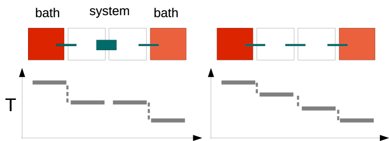
Figure 1: When the system-bath coupling is weak but the coupling inside the system is not weak, we expect a flat temperature profile because the thermal resistance is large only at the boundaries. If the coupling in the system is also weak, we expect a nonzero temperature gradient in the system.

Heat-conducting states with nonzero temperature gradients are difficult to study analytically, because they are usually realized in non-integrable systems. However, our setting allows some analytical treatment of such states. In this paper, we consider one-dimensional uniform quantum spin-1/2 systems with nearest-neighbor interactions, whose Hamiltonians are of the form

$$H = \lambda\sum_{l}\sum_{j,k}\alpha_{j,k}\sigma_{l}^{j}\sigma_{l+1}^{k}+h\sum_{l}\sigma_{l}^{z}.$$ (1)

Here, $\sigma_{l}^{j}\;(j=x,y,z)$ represents a Pauli matrix at the $l$th site. We assume $h\neq 0$ and $\alpha_{ij}=\alpha_{ji}$. Then we show that

$$\alpha_{zz}\neq 0$$ (2)

is necessary to form a nonzero temperature gradient. Note that this condition is independent of the integrability of the system. For example, it is consistent with the observation that the $XXZ$ model has normal conducting states in spite of its integrabilityprosen ; michel ; wu ; mendoza . We can understand intuitively that Eq. (2) must be satisfied so that the local temperature at a site can affect the temperatures of neighboring sites, because in the weak-coupling limit the local temperature is determined only from $\langle\sigma_{z}\rangle$. We also show that some three-body correlations play important roles in forming the temperature gradient. The forms of the correlation terms are universal, i.e., they do not depend on the form of the interaction.

This paper is organized as follows. In Sect. II, we derive the quantum master equation (QME) in the weak-coupling limit. We show that the heat bath superoperator becomes local when the spin-spin coupling is weak. In Sect. III, we derive a perturbative expansion of the stationary solution of the QME. In Sect. IV we study quantum spin-1/2 chains. First we analyze two-spin cases and show an explicit example of a frozen NESS with a nonzero temperature gradient. Then we study $N$-spin systems and derive Eq. (2). We also show some numerical results to verify our theoretical considerations. Section V is devoted to a summary.

II Quantum Master Equation

In this section, we derive the QME for weakly coupled spin systems. For simplicity, we first derive the QME for a system coupled to a single heat bath. Generalization to multiple heat baths is straightforward. We denote the Hilbert space of the system by $\mathsf{H}$ and assume that its dimension is finite. The set of all linear operators on $\mathsf{H}$ is denoted by $\mathsf{L}$. It becomes a Hilbert space by introducing the Hilbert–Schmidt inner product as ${\rm Tr}\left(X_{1}X_{2}\right)$ for any $X_{1},X_{2}\in\mathsf{L}$. We refer to a linear operator on $\mathsf{L}$ as a superoperator.

We start with the Hamiltonian

$$H = H_{\rm S}+H_{\rm B}+\lambda H_{\rm SB},$$ (3)

where $\lambda$ is a small coupling parameter, $H_{\rm S}$ is the Hamiltonian for the system, and $H_{\rm B}$ is that for the heat bath. $H_{\rm SB}$ represents the interaction between the system and the heat bath, which can be written as

$$H_{\rm SB} = \sum_{j}X_{j}Y_{j}.$$ (4)

Here, $X_{j}$ and $Y_{j}$ are Hermitian operators on the system and on the heat bah, respectively. By using the Born-Markov approximationkubo ; breuer , we obtain the standard Redfield-type QME

$$\frac{d}{dt}\rho(t) = \frac{1}{i\hbar}\left[H_{\rm S},\rho(t)\right]+\lambda\frac{1}{i\hbar}\left[\overline{H}_{\rm SB},\rho(t)\right]+\lambda^{2}\mathcal{D}\rho.$$ (5)

Here, $\overline{H}_{\rm SB}\in\mathsf{L}$ represents the interaction averaged over the heat bath, whose explicit form is

$$\overline{H}_{SB} = {\rm Tr}_{\rm B}H_{\rm SB}=\sum_{j}X_{j}\overline{Y}_{j},$$ (6)

where $\overline{Y}_{j}={\rm Tr}\left\{\rho_{\rm B}Y_{j}\right\}$ and $\rho_{\rm B}$ is the equilibrium state of the heat bath $\rho_{\rm B}=e^{-\beta H_{\rm B}}/Z_{\rm B}$. $\mathcal{D}$ is the heat bath superoperator

$$\mathcal{D}\rho = -\frac{1}{\hbar^{2}}\sum_{jl}\left[X_{j},S_{jl}\rho\right]+{\rm h.c.},$$ (7)

where

$$S_{jl} = \int_{0}^{\infty}dte^{-iH_{\rm S}t/\hbar}X_{l}e^{iH_{\rm S}t/\hbar}\Phi_{jl}(t).$$ (8)

$\Phi_{jl}$ is a correlation function for the heat bath,

$$\Phi_{jl}(t) = {\rm Tr}\left\{\rho_{\rm B}\Delta Y_{j}(t)\Delta Y_{l}\right\},$$ (9)

where $\Delta Y_{k}(t)=Y_{k}(t)-\overline{Y}_{k}$. Note that Eq. (5) is correct up to $O(\lambda^{2})$. We also use the Markovian approximation in deriving Eq. (5), which is correct when the density matrix in the interacting picture $e^{iH_{\rm S}t/\hbar}\rho(t)e^{-iH_{\rm S}t/\hbar}$ is slowly varying compared with the correlation time of the heat bath kubo . This assumption holds for NESSs in a weakly nonequilibrium regime. In our perturbation theory, the zeroth order solution satisfies this condition exactly even when it is far from equilibrium.

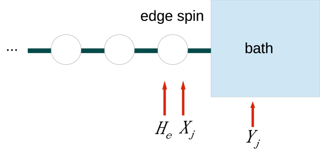
Figure 2: $X_{j}$ and $H_{\rm e}$ act only on the edge spin.

Now we consider a weakly coupled one-dimensional spin system with nearest-neighbor interactions. We assume that the spin-spin interaction is of the same order as the system-bath interaction. Then the system Hamiltonian can be written as

$$H_{\rm S} = H_{0}+\lambda H_{\rm I},$$ (10)

where $H_{0}$ represents the external field applied to the spins and $H_{\rm I}$ is the interaction among the spins. We also assume that the $X_{j}$ in $H_{\rm SB}$ act only on the edge spin (Fig. 2) and write

$$H_{0} = H_{0}^{\prime}+H_{\rm e},$$ (11)

where $H_{\rm e}$ acts on the edge spin and $H_{0}^{\prime}$ acts on the other spins. Since $[H_{0}^{\prime},X_{j}]=0$, we have

$$S_{jl} = \int_{0}^{\infty}dte^{-iH_{\rm e}t/\hbar}X_{l}e^{iH_{\rm e}t/\hbar}\Phi_{jl}(t)+O(\lambda).$$ (12)

The $O(\lambda)$ term is negligible in the QME in Eq. (5), and now $S_{jl}$ is a local operator acting on the edge spin. It can also be written as

$$S_{jl} = \sum_{pq}\Xi_{jl}\left(\frac{E_{p}-E_{q}}{\hbar}\right)|E_{p}\rangle\langle E_{p}|X_{l}|E_{q}\rangle\langle E_{q}|,$$ (13)

where $\Xi_{jl}$ is the Fourier–Laplace transform of the correlation function

$$\Xi_{jl}(\omega) = \int_{0}^{\infty}e^{-i\omega t}\Phi_{jl}(t),$$ (14)

$E_{r}$ is an eigenvalue of $H_{\rm e}$ and $|E_{r}\rangle$ is the corresponding eigenvector.

If we place heat baths at both ends of the spin chain, the QME for this weak-coupling limit is

$$\frac{d}{dt}\rho = \mathcal{L}\rho,$$ (15)

$$\mathcal{L} = \mathcal{L}_{0}+\lambda\mathcal{L}_{1}+\lambda^{2}\mathcal{L}_{2},$$ (16)

$$\mathcal{L}_{0}\rho = \frac{1}{i\hbar}[H_{0},\rho],$$ (17)

$$\mathcal{L}_{1}\rho = \frac{1}{i\hbar}[H_{1},\rho],$$ (18)

$$\mathcal{L}_{2}\rho = \mathcal{D}_{\rm L}\rho+\mathcal{D}_{\rm R}\rho,$$ (19)

where $H_{1}=H_{\rm I}+\overline{H}_{\rm SB}$, and $\mathcal{D}_{\rm L}$ and $\mathcal{D}_{\rm R}$ are heat bath superoperators for the left and right heat baths, respectively. They are of the form given in Eqs. (7) and (13).

III Perturbative Expansion

III.1 Zeroth-order solution

The steady state is determined by the equation

$$\frac{d}{dt}\rho=\mathcal{L}\rho=0.$$ (20)

We calculate the steady state by expanding $\rho$ with respect to the coupling parameter $\lambda$:

$$\rho = \rho_{0}+\lambda\rho_{1}+\lambda^{2}\rho_{2}+\dots.$$ (21)

By substituting it into Eq. (20), we obtain the following equations up to the second order:

$$\mathcal{L}_{0}\rho_{0} = 0,$$ (22)

$$\mathcal{L}_{0}\rho_{1}+\mathcal{L}_{1}\rho_{0} = 0,$$ (23)

$$\mathcal{L}_{0}\rho_{2}+\mathcal{L}_{1}\rho_{1}+\mathcal{L}_{2}\rho_{0} = 0.$$ (24)

In usual perturbation theories, the zeroth-order solution is determined from the zeroth-order equation. In this case, however, we cannot determine $\rho_{0}$ simply from Eq. (22), and the first order-equation Eq. (23) also fails to determine $\rho_{0}$. Hence we need all three equations Eqs. (22)-(24) to determine the zeroth-order solution. Physically speaking, this is because the Liouvillian $\mathcal{L}_{0}+\lambda\mathcal{L}_{1}$ represents Hamiltonian dynamics governed by $H_{0}+\lambda H_{1}$, and all energy eigenstates of $H_{0}+\lambda H_{1}$ are stationary in this dynamics. We require the heat baths, which are represented by $\mathcal{L}_{2}$, to make the stationary state unique.

Let us consider the eigenvalue problem of the Hamiltonian $H_{0}+\lambda H_{1}$ up to the first order of $\lambda$. Since $H_{0}$ is a non-interacting Hamiltonian and highly degenerate, we must use degenerate perturbation theory. Then we obtain the eigenvalues

$$E_{n,k} = E_{n}+\lambda e^{(n)}_{k},$$ (25)

where $E_{n}$ is an eigenvalue of $H_{0}$ and $e^{(n)}_{k}$ is obtained by diagonalizing $H_{1}$ in the eigenspace belonging to $E_{n}$. Therefore, the corresponding eigenvector $|E_{n,k}\rangle$ satisfies

$$H_{0}|E_{n,k}\rangle = E_{n}|E_{n,k}\rangle$$ (26)

and

$$\langle E_{n,k}|H_{1}|E_{n,l}\rangle = e^{(n)}_{k}\delta_{k,l}.$$ (27)

We assume the $E_{n,k}$ are nondegenerate.

Since $|E_{n,k}\rangle\langle E_{m,l}|\in\mathsf{L}$ satisfies the equation

$$\mathcal{L}_{0}|E_{n,k}\rangle\langle E_{m,l}| = \frac{E_{n}-E_{m}}{i\hbar}|E_{n,k}\rangle\langle E_{m,l}|,$$ (28)

it is an eigenoperator of $\mathcal{L}_{0}$ with the eigenvalue $\frac{E_{n}-E_{m}}{i\hbar}$, and the operators of this type form a complete set in $\mathsf{L}$. The zero eigenspace is spanned by the operators with $n=m$:

$$\mathtt{Ker\,}\mathcal{L}_{0} = \tt{Span}\left\{|E_{n,k}\rangle\langle E_{n,l}|\right\}_{n,k,l}.$$ (29)

We denote the projection superoperator to $\mathtt{Ker\,}\mathcal{L}_{0}$ by $\mathcal{P}_{0}$. Then we have

$$\mathcal{P}_{0}\mathcal{L}_{0}=\mathcal{L}_{0}\mathcal{P}_{0}=0$$ (30)

and

$$\mathcal{P}_{0}\rho_{0}=\rho_{0}$$ (31)

because $\rho_{0}\in\mathtt{Ker\,}\mathcal{L}_{0}$. By applying $\mathcal{P}_{0}$ to Eq. (23), we obtain

$$\mathcal{P}_{0}\mathcal{L}_{1}\rho_{0}=\mathcal{P}_{0}\mathcal{L}_{1}\mathcal{P}_{0}\rho_{0}=0.$$ (32)

Hence, $\rho_{0}$ is in $\mathtt{Ker\,}\left(\mathcal{P}_{0}\mathcal{L}_{1}\mathcal{P}_{0}\right)$, which is spanned by the diagonal elements:

$$\mathtt{Ker\,}\left(\mathcal{P}_{0}\mathcal{L}_{1}\mathcal{P}_{0}\right) = \tt{Span}\left\{|E_{n,k}\rangle\langle E_{n,k}|\right\}_{n,k}.$$ (33)

We denote the projection superoperator to $\mathtt{Ker\,}\left(\mathcal{P}_{0}\mathcal{L}_{1}\mathcal{P}_{0}\right)$ by $\mathcal{P}_{1}$. Then

$$\mathcal{P}_{1}\rho_{0}=\rho_{0}.$$ (34)

We also define projection superoperators

$$\mathcal{Q}_{0} \coloneqq 1-\mathcal{P}_{0},$$ (35)

$$\mathcal{Q}_{1} \coloneqq \mathcal{P}_{0}-\mathcal{P}_{1}.$$ (36)

Note that

$$1=\mathcal{Q}_{0}+\mathcal{Q}_{1}+\mathcal{P}_{1}$$ (37)

and $\mathtt{Im\,}\mathcal{P}_{1}\subset\mathtt{Im\,}\mathcal{P}_{0}$, $\mathtt{Im\,}\mathcal{Q}_{1}\subset\mathtt{Im\,}\mathcal{P}_{0}$.

Applying $\mathcal{Q}_{0}$ to Eq. (23), we obtain

$$Q_{0}\mathcal{L}_{0}(P_{0}+Q_{0})\rho_{1}+Q_{0}\mathcal{L}_{1}\rho_{0}=Q_{0}\mathcal{L}_{0}Q_{0}\rho_{1}+Q_{0}\mathcal{L}_{1}\rho_{0}=0.$$ (38)

Hence,

$$\mathcal{Q}_{0}\rho_{1} = -\left(Q_{0}\mathcal{L}_{0}Q_{0}\right)^{-1}\mathcal{L}_{1}\rho_{0}.$$ (39)

Note that the superoperator $\left(Q_{0}\mathcal{L}_{0}Q_{0}\right)^{-1}$ is defined on ${\tt Im}Q_{0}$. We implicitly assumed in Eq. (39) that $\left(Q_{0}\mathcal{L}_{0}Q_{0}\right)^{-1}\rho=0$ if $\rho\notin{\tt Im}Q_{0}$. Hence,

$$\left(Q_{0}\mathcal{L}_{0}Q_{0}\right)^{-1}=\left(Q_{0}\mathcal{L}_{0}Q_{0}\right)^{-1}Q_{0}.$$ (40)

By applying $\mathcal{P}_{1}$ to Eq. (24), we obtain

$$\mathcal{P}_{1}\mathcal{L}_{1}\rho_{1}+\mathcal{P}_{1}\mathcal{L}_{2}\rho_{0}=0.$$ (41)

Since $\mathcal{P}_{1}\mathcal{L}_{1}\mathcal{P}_{0}=\mathcal{P}_{1}\mathcal{P}_{0}\mathcal{L}_{1}\mathcal{P}_{0}=0$, we have

$$\mathcal{P}_{1}\mathcal{L}_{1}\rho_{1} = \mathcal{P}_{1}\mathcal{P}_{0}\mathcal{L}_{1}(\mathcal{P}_{0}+\mathcal{Q}_{0})\rho_{1}$$ (42)

$$= -\mathcal{P}_{1}\mathcal{L}_{1}\left(Q_{0}\mathcal{L}_{0}Q_{0}\right)^{-1}\mathcal{L}_{1}\mathcal{P}_{1}\rho_{0}.$$ (43)

We can show that

$$\mathcal{P}_{1}\mathcal{L}_{1}\left(Q_{0}\mathcal{L}_{0}Q_{0}\right)^{-1}\mathcal{L}_{1}\mathcal{P}_{1}=0$$ (44)

by a straightforward algebra (see AppendixA). Hence, we obtain the following three equations to determine the zeroth-order solution:

$$\mathcal{L}_{0}\rho_{0} = 0,$$ (45)

$$\mathcal{P}_{0}\mathcal{L}_{1}\rho_{0} = 0,$$ (46)

$$\mathcal{P}_{1}\mathcal{L}_{2}\rho_{0} = 0.$$ (47)

III.2 Higher-order solutions

In a similar way, we can obtain higher-order solutions. If the Liouvillian is expanded with respect to $\lambda$ as

$$\mathcal{L} = \sum_{n=0}^{\infty}\lambda^{n}\mathcal{L}_{n},$$ (48)

the $m$th-order equation is

$$\sum_{n=0}^{m}\mathcal{L}_{n}\rho_{m-n} = 0.$$ (49)

We decompose the $m$th-order solution as

$$\rho_{m} = \mathcal{Q}_{0}\rho_{m}+\mathcal{Q}_{1}\rho_{m}+\mathcal{P}_{1}\rho_{m}$$ (50)

and represent the three terms by lower-order solutions in the following.

First we apply $\mathcal{Q}_{0}$ to Eq. (49). Then we have

$$\mathcal{Q}_{0}\mathcal{L}_{0}\rho_{m} = -Q_{0}\sum_{n=1}^{m}\mathcal{L}_{n}\rho_{m-n}.$$ (51)

Hence,

$$\mathcal{Q}_{0}\rho_{m} = -\left(Q_{0}\mathcal{L}_{0}Q_{0}\right)^{-1}\sum_{n=1}^{m}\mathcal{L}_{n}\rho_{m-n}.$$ (52)

Then we apply $\mathcal{Q}_{1}$ to the $(m+1)$th-order equation. Since $\mathcal{Q}_{1}\mathcal{L}_{0}=0$, we have

$$\mathcal{Q}_{1}\mathcal{L}_{1}\rho_{m} = -\mathcal{Q}_{1}\sum_{n=2}^{m+1}\mathcal{L}_{n}\rho_{m+1-n}.$$ (53)

Because

$$Q_{1}\mathcal{L}_{1}=Q_{1}\mathcal{L}_{1}(P_{1}+Q_{1}+Q_{0})=Q_{1}\mathcal{L}_{1}(Q_{1}+Q_{0}),$$ (54)

we obtain

$$Q_{1}\rho_{m} = -\left(Q_{1}\mathcal{L}_{1}Q_{1}\right)^{-1}\left(\mathcal{L}_{1}Q_{0}\rho_{m}+\sum_{n=2}^{m+1}\mathcal{L}_{n}\rho_{m+1-n}\right).$$ (55)

Next we apply $\mathcal{P}_{1}$ to the $(m+2)$th-order equation. Then we have

$$\mathcal{P}_{1}\mathcal{L}_{1}\rho_{m+1}+\mathcal{P}_{1}\mathcal{L}_{2}\rho_{m}+\mathcal{P}_{1}\sum_{n=3}^{m+2}\mathcal{L}_{n}\rho_{m+2-n} = 0.$$ (56)

The first term is

$$\mathcal{P}_{1}\mathcal{L}_{1}(\mathcal{P}_{0}+\mathcal{Q}_{0})\rho_{m+1} = \mathcal{P}_{1}\mathcal{L}_{1}\mathcal{Q}_{0}\rho_{m+1}$$ (57)

$$= -\mathcal{P}_{1}\mathcal{L}_{1}\left(Q_{0}\mathcal{L}_{0}Q_{0}\right)^{-1}\left(\mathcal{L}_{1}\rho_{m}+\sum_{n=2}^{m+1}\mathcal{L}_{n}\rho_{m+1-n}\right)$$ (58)

$$= -\mathcal{P}_{1}\mathcal{L}_{1}\left(Q_{0}\mathcal{L}_{0}Q_{0}\right)^{-1}\left(\mathcal{L}_{1}(\mathcal{Q}_{1}+\mathcal{Q}_{0})\rho_{m}+\sum_{n=2}^{m+1}\mathcal{L}_{n}\rho_{m+1-n}\right),$$ (59)

where we used Eq. (52) with $m$ replaced by $m+1$ in the second line and Eq. (44) in the last line. Therefore,

$$\mathcal{P}_{1}\mathcal{L}_{2}\mathcal{P}_{1}\rho_{m}+\mathcal{P}_{1}\left(\mathcal{L}_{2}-\mathcal{L}_{1}\left(Q_{0}\mathcal{L}_{0}Q_{0}\right)^{-1}\mathcal{L}_{1}\right)(\mathcal{Q}_{1}+\mathcal{Q}_{0})\rho_{m}$$ (60)

$$+\mathcal{P}_{1}\sum_{n=2}^{m+1}\left(\mathcal{L}_{n+1}-\mathcal{L}_{1}(\mathcal{Q}_{0}\mathcal{L}_{0}\mathcal{Q}_{0})^{-1}\mathcal{L}_{n}\right)\rho_{m+1-n} = 0.$$ (61)

The superoperator $\mathcal{P}_{1}\mathcal{L}_{2}\mathcal{P}_{1}$ is not invertible since it has a one-dimensional kernel spanned by $\rho_{0}$. Therefore, we define $\left(\mathcal{P}_{1}\mathcal{L}_{2}\mathcal{P}_{1}\right)^{-1}$ as the Moore-Penrose pseudoinverse of $\mathcal{P}_{1}\mathcal{L}_{2}\mathcal{P}_{1}$. Then we have

$$\mathcal{P}_{1}\rho_{m} = \left(\mathcal{P}_{1}\mathcal{L}_{2}\mathcal{P}_{1}\right)^{-1}\left\{\left(\mathcal{L}_{1}\left(Q_{0}\mathcal{L}_{0}Q_{0}\right)^{-1}\mathcal{L}_{1}-\mathcal{L}_{2}\right)(\mathcal{Q}_{1}+\mathcal{Q}_{0})\rho_{m}+\sum_{n=2}^{m+1}\left(\mathcal{L}_{1}(\mathcal{Q}_{0}\mathcal{L}_{0}\mathcal{Q}_{0})^{-1}\mathcal{L}_{n}-\mathcal{L}_{n+1}\right)\rho_{m+1-n}\right\}$$ (62)

$$+c\rho_{0},$$

where the constant $c$ is determined by the condition

$${\rm Tr}\rho_{m} = 0\;\;\;\;(m\geq 1).$$ (63)

Combining Eqs. (52), (55), and (62), we obtain the $m$th-order solution $\rho_{m}$. For example, the first-order solution is given by

$$\rho_{1} = \mathcal{Q}_{0}\rho_{1}+\mathcal{Q}_{1}\rho_{1}+\mathcal{P}_{1}\rho_{1},$$ (64)

$$\mathcal{Q}_{0}\rho_{1} = -(\mathcal{Q}_{0}\mathcal{L}_{0}\mathcal{Q}_{0})^{-1}\mathcal{L}_{1}\rho_{0},$$ (65)

$$\mathcal{Q}_{1}\rho_{1} = -(\mathcal{Q}_{1}\mathcal{L}_{1}\mathcal{Q}_{1})^{-1}\left(\mathcal{L}_{1}\mathcal{Q}_{0}\rho_{1}+\mathcal{L}_{2}\rho_{0}\right),$$ (66)

$$\mathcal{P}_{1}\rho_{1} = \left(\mathcal{P}_{1}\mathcal{L}_{2}\mathcal{P}_{1}\right)^{-1}\left\{\left(\mathcal{L}_{1}\left(\mathcal{Q}_{0}\mathcal{L}_{0}\mathcal{Q}_{0}\right)^{-1}\mathcal{L}_{1}-\mathcal{L}_{2}\right)(\mathcal{Q}_{1}+\mathcal{Q}_{0})\rho_{1}+\left(\mathcal{L}_{1}\left(\mathcal{Q}_{0}\mathcal{L}_{0}\mathcal{Q}_{0}\right)^{-1}\mathcal{L}_{2}-\mathcal{L}_{3}\right)\rho_{0}\right\}$$ (67)

$$+c\rho_{0}.$$

Here, we give some comments about the range of applicability of our perturbation theory. Our method has two parameters, the system size and the coupling constant, which compete with each other. If the system size is large, $\mathcal{Q}_{1}\rho_{m}$ may be very large because we have $(\mathcal{Q}_{1}\mathcal{L}_{1}\mathcal{Q}_{1})^{-1}$ in Eq. (55), whose eigenvalues may be very large. Then our method could work only for a very small coupling constant $\lambda$ and might be practically useless for large systems. However, it is also possible that even when the higher-order terms of the density matrix are large, they give only small contributions to local physical quantities such as local temperature and current. (Note that very different states, such as a pure state and the Gibbs state, can give the same expectation values for local observables in macroscopic systems sugita2 ; sugiura .) Then our method may be useful even for large systems.

To consider this point, we will give some numerical results for spin systems in the next section. The results show that, for local temperatures, the zeroth-order approximation is equally good for the system sizes $N=2$ and $N=6$. Therefore, we hope that our method is useful for larger systems.

Another important point to note is that a NESS in a rather small system may be similar to a part of a macroscopic NESS, at least in some aspects. Thus, we will be able to obtain some insights on macroscopic NESSs by studying those in small systems, where our method will be helpful.

IV Spin-1/2 Chain

In this section, we consider a quantum $N$-spin chain with the Hamiltonian

$$H_{\rm S} = H_{0}+\lambda H_{\rm I},$$ (68)

$$H_{0} = h\sum_{l=1}^{N}\sigma_{l}^{z},$$ (69)

$$H_{\rm I} = \sum_{l=1}^{N-1}\sum_{j,k}\alpha_{j,k}\sigma^{j}_{l}\sigma^{k}_{l+1}.$$ (70)

In this section we set $\hbar=1$.

IV.1 Basis of $\mathtt{Ker\,}\mathcal{L}_{0}$

We represent spin up and down states by $|1\rangle$ and $|-1\rangle$, respectively. Then $H_{0}$ has eigenvectors of the form

$$|\{s_{l}\}\rangle \coloneqq |s_{1}\rangle\otimes|s_{2}\rangle\otimes\dots\otimes|s_{N}\rangle,$$ (71)

where $s_{l}=\pm 1$, and its eigenvalue is $h\sum_{l}s_{l}$. $\mathtt{Ker\,}\mathcal{L}_{0}$ is spanned by elements of the form

$$|\{s_{l}\}\rangle\langle\{s^{\prime}_{l}\}|$$ (72)

with

$$\sum_{l}s_{l}=\sum_{l}s^{\prime}_{l}.$$ (73)

Note that the number of sites with $s_{l}\neq s^{\prime}_{l}$ must be even to satisfy this condition.

Let us consider some simple cases. If $N=1$, $\mathtt{Ker\,}\mathcal{L}_{0}$ is spanned by $|1\rangle\langle 1|$ and $|-1\rangle\langle-1|$. In this case, only diagonal terms appear. Therefore, in this case, $\mathtt{Ker\,}\mathcal{L}_{0}$ is spanned by $\sigma^{0}$ and $\sigma^{z}$, where $\sigma^{0}$ is the $2\times 2$ unit matrix.

If $N=2$, $\mathtt{Ker\,}\mathcal{L}_{0}$ is spanned by six elements, in which there are four diagonal elements,

$$|1,1\rangle\langle 1,1|,\;\;\;|1,-1\rangle\langle 1,-1|,\;\;\;|-1,1\rangle\langle-1,1|,\;\;\;|-1,-1\rangle\langle-1,-1|,$$ (74)

and two off-diagonal elements,

$$|1,-1\rangle\langle-1,1|,\;\;\;|-1,1\rangle\langle 1,-1|.$$ (75)

The diagonal terms can be represented by linear combinations of $\sigma_{\alpha}\otimes\sigma_{\beta}$, where $\alpha,\beta$ are $0$ or $z$. The off-diagonal terms are represented as

$$|1,-1\rangle\langle-1,1| = \sigma_{1}^{+}\otimes\sigma_{2}^{-}=\frac{1}{4}\left\{(\sigma_{1}^{x}\otimes\sigma_{2}^{x}+\sigma_{1}^{y}\otimes\sigma_{2}^{y})-i(\sigma_{1}^{x}\otimes\sigma_{2}^{y}-\sigma_{1}^{y}\otimes\sigma_{2}^{x})\right\}$$ (76)

$$|-1,1\rangle\langle 1,-1| = \sigma_{1}^{-}\otimes\sigma_{2}^{+}=\frac{1}{4}\left\{(\sigma_{1}^{x}\otimes\sigma_{2}^{x}+\sigma_{1}^{y}\otimes\sigma_{2}^{y})+i(\sigma_{1}^{x}\otimes\sigma_{2}^{y}-\sigma_{1}^{y}\otimes\sigma_{2}^{x})\right\}$$ (77)

where

$$\sigma_{l}^{\pm}=\frac{1}{2}(\sigma_{l}^{x}\pm i\sigma_{l}^{y}).$$ (78)

Therefore, the off-diagonal terms can be represented by the two terms $\sigma_{1}^{x}\otimes\sigma_{2}^{x}+\sigma_{1}^{y}\otimes\sigma_{2}^{y}$ and $\sigma_{1}^{x}\otimes\sigma_{2}^{y}-\sigma_{1}^{y}\otimes\sigma_{2}^{y}$.

For the $N$-spin case, a basis element in Eq. (72) has an even number of off-diagonal sites where $s_{l}\neq s^{\prime}_{l}$. The diagonal parts can be represented by combining $\sigma_{0}$ and $\sigma_{z}$, and the off-diagonal parts can be obtained by combining the following two types of correlation terms:

$$\rho^{\rm A}_{l,m} \coloneqq \sigma_{l}^{x}\otimes\sigma_{m}^{x}+\sigma_{l}^{y}\otimes\sigma_{m}^{y},$$ (79)

$$\rho^{\rm B}_{l,m} \coloneqq \sigma_{l}^{x}\otimes\sigma_{m}^{y}-\sigma_{l}^{y}\otimes\sigma_{m}^{x}.$$ (80)

IV.2 Zeroth-order solution for the two-spin case

Let us consider the two-spin case. In this case $\mathtt{Ker\,}\mathcal{L}_{0}$ is six dimensional, and we take the basis as

$$\mathtt{Ker\,}\mathcal{L}_{0} = \mathtt{Span\,}\left\{\sigma^{00},\sigma^{zz},\sigma^{0z}+\sigma^{z0},\rho^{\rm A},\rho^{\rm B},\rho^{\rm C}\right\}.$$ (81)

Here we used the notation

$$\sigma^{jk} \coloneqq \sigma_{1}^{j}\otimes\sigma_{2}^{k}.$$ (82)

$\rho^{\rm A}$ and $\rho^{\rm B}$ are correlation terms in the form of Eqs. (79) and (80), respectively, with $l=1$ and $m=2$. $\rho^{\rm C}$ is defined as

$$\rho^{\rm C} \coloneqq \sigma^{0z}-\sigma^{z0}.$$ (83)

Then we consider Eq. (46). $\mathcal{L}_{1}$ is represented by two terms,

$$\mathcal{L}_{1} = \mathcal{L}_{\rm I}+\mathcal{L}_{\rm E},$$ (84)

where

$$\mathcal{L}_{\rm I}\rho = -i[H_{\rm I},\rho],$$ (85)

$$\mathcal{L}_{\rm E}\rho = -i[\overline{H}_{SB},\rho].$$ (86)

By straightforward algebra, we obtain

$$\mathcal{P}_{0}\mathcal{L}_{\rm I}\sigma^{00}=\mathcal{P}_{0}\mathcal{L}_{\rm I}\sigma^{zz}=\mathcal{P}_{0}\mathcal{L}_{\rm I}(\sigma^{0z}+\sigma^{z0})=0,$$ (87)

$$\mathcal{P}_{0}\mathcal{L}_{\rm I}\rho^{\rm A} = 0,$$ (88)

$$\mathcal{P}_{0}\mathcal{L}_{\rm I}\rho^{\rm B} = 2\alpha_{+}\rho^{\rm C},$$ (89)

$$\mathcal{P}_{0}\mathcal{L}_{\rm I}\rho^{\rm C} = -2\alpha_{+}\rho^{\rm B},$$ (90)

where $\alpha_{+}\coloneqq\alpha_{xx}+\alpha_{yy}$.

We write

$$\overline{H}_{\rm SB} = \sum_{j=x,y,z}(\alpha_{\rm L}^{j}\sigma^{j0}+\alpha_{\rm R}^{j}\sigma^{0j}),$$ (91)

which represents the first-order effect of the system-bath coupling from the left and right heat baths. Then we have

$$\mathcal{P}_{0}\mathcal{L}_{\rm E}\sigma^{00}=\mathcal{P}_{0}\mathcal{L}_{\rm E}\sigma^{zz}=\mathcal{P}_{0}\mathcal{L}_{\rm E}(\sigma^{0z}+\sigma^{z0})=0,$$ (92)

$$\mathcal{P}_{0}\mathcal{L}_{\rm E}\rho^{\rm A} = -2\Delta\alpha^{z}\rho^{\rm B},$$ (93)

$$\mathcal{P}_{0}\mathcal{L}_{\rm E}\rho^{\rm B} = 2\Delta\alpha^{z}\rho^{\rm A},$$ (94)

$$\mathcal{P}_{0}\mathcal{L}_{\rm E}\rho^{\rm C} = 0,$$ (95)

where $\Delta\alpha^{z}\coloneqq\alpha_{\rm L}^{z}-\alpha_{\rm R}^{z}$. Therefore, we have

$$\mathtt{Ker\,}\mathcal{P}_{0}\mathcal{L}_{1}\mathcal{P}_{0} = \mathtt{Span\,}\left\{\sigma^{00},\sigma^{zz},\sigma^{0z}+\sigma^{z0},\rho^{C^{\prime}}\right\},$$ (96)

where

$$\rho^{C^{\prime}} \coloneqq \rho^{\rm C}-\gamma\rho^{\rm A},$$ (97)

$$\gamma \coloneqq \frac{\alpha_{+}}{\Delta\alpha_{z}}.$$ (98)

Let us consider the local equilibrium form

$$\rho_{\rm LE}(\beta_{1})\otimes\rho_{\rm LE}(\beta_{2}).$$ (99)

Here, $\rho_{\rm LE}$ represents a single-spin equilibrium state, whose explicit form is

$$\rho_{\rm LE}(\beta_{l})=\frac{e^{-\beta_{l}h\sigma^{z}}}{e^{\beta_{l}h}+e^{-\beta_{l}h}}=\frac{1}{2}(\sigma^{0}-t_{l}\sigma^{z}),$$ (100)

where $t_{l}\coloneqq\tanh(\beta_{l}h)$. Then we apply $\mathcal{P}_{0}\mathcal{L}_{1}$ to Eq. (99). Since

$$\rho_{\rm LE}(\beta_{1})\otimes\rho_{\rm LE}(\beta_{2}). = \frac{1}{4}\left\{\sigma^{00}+t_{1}t_{2}\sigma^{zz}-\frac{t_{1}+t_{2}}{2}(\sigma^{0z}+\sigma^{z0})-\frac{t_{2}-t_{1}}{2}\rho^{\rm C}\right\},$$ (101)

we have

$$\mathcal{P}_{0}\mathcal{L}_{1}\rho_{\rm LE}(\beta_{1})\otimes\rho_{\rm LE}(\beta_{2}) = \frac{t_{2}-t_{1}}{4}\alpha_{+}\rho^{\rm B}.$$ (102)

Therefore, we see that the local equilibrium form in Eq. (99) is not the zeroth-order solution unless $t_{1}=t_{2}$. The general form of the solution of the equation $\mathcal{P}_{0}\mathcal{L}_{1}\rho_{0}=0$ is

$$\rho_{0} = \rho_{\rm LE}(\beta_{1})\otimes\rho_{\rm LE}(\beta_{2})+\frac{t_{2}-t_{1}}{8}\gamma\rho^{\rm A}+g\sigma^{zz},$$ (103)

where the three parameters $t_{1},t_{2}$, and $g$ are to be determined from $\mathcal{P}_{1}\mathcal{L}_{2}\rho_{0}=0$. Note that the correlation term $\rho^{\rm A}$ appears when there is a temperature gradient in the system.

Let us consider the tilted Ising model as an example:

$$H = \lambda\sigma^{zz}+h\cos\theta(\sigma^{z0}+\sigma^{0z})+h\sin\theta(\sigma^{x0}+\sigma^{0x}).$$ (104)

This model is known to be integrable at $\theta=\pi/2$ (transverse Ising model), and the NESS has a flat temperature profile in this case saito1 .

By taking the $z$-axis in the direction of the external field, the Hamiltonian can be transformed as

$$H = \lambda\sigma_{1}^{z^{\prime}}\otimes\sigma_{2}^{z^{\prime}}+h(\sigma^{z0}+\sigma^{0z}),$$ (105)

where

$$\sigma_{l}^{z^{\prime}} \coloneqq \sigma_{l}^{z}\cos\theta-\sigma_{l}^{x}\sin\theta.$$ (106)

The interaction term can also be written as

$$\sigma_{1}^{z^{\prime}}\otimes\sigma_{2}^{z^{\prime}} = \sigma^{zz}\cos^{2}\theta-(\sigma^{zx}+\sigma^{xz})\cos\theta\sin\theta+\sigma^{xx}\sin^{2}\theta.$$ (107)

Therefore, we have

$$\alpha_{zz} = \cos^{2}\theta$$ (108)

$$\alpha_{zx}=\alpha_{xz} = -\cos\theta\sin\theta$$ (109)

$$\alpha_{xx} = \sin^{2}\theta.$$ (110)

We take the spin-bath coupling as having the same form as the spin-spin coupling (Fig. 3). This situation may be regarded as similar to that for the two spins in a NESS of a long spin chain. We also assume that the temperature difference between the two heat baths is small. Then we obtain

$$t_{1} = \frac{t_{\rm L}+t_{\rm R}}{2}+\frac{K}{2}(t_{\rm L}-t_{\rm R}),$$ (111)

$$t_{2} = \frac{t_{\rm L}+t_{\rm R}}{2}-\frac{K}{2}(t_{\rm L}-t_{\rm R}),$$ (112)

$$g = -\frac{K(1-K)}{16}(t_{\rm L}-t_{\rm R})^{2},$$ (113)

where $t_{l}=\tanh(\beta_{l}h)\;\;(l={\rm L,R})$, and $\beta_{\rm L}$ ($\beta_{\rm R}$) is the inverse temperature for the left (right) heat bath. $K$ is defined as

$$K \coloneqq \frac{c(t_{\rm L}-t_{\rm R})^{2}\cos^{4}\theta}{c(t_{\rm L}-t_{\rm R})^{2}\cos^{4}\theta+\sin^{2}\theta(2d\cos^{2}\theta+c\sin^{2}\theta)},$$ (114)

where $c$ and $d$ are non-negative constants. (See AppendixB for details of the calculation.) We see that a nonzero temperature gradient is formed unless $\alpha_{zz}=\cos^{2}\theta=0$, which corresponds to the transverse Ising model.

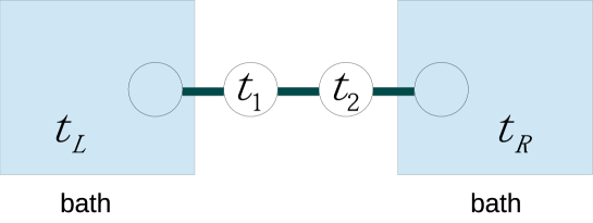
Figure 3: Schematic figure of our two-spin model. The system-bath coupling is assumed to have the same form as the spin-spin coupling. The $t_{l}$ are related to the local inverse temperatures by $t_{l}=\tanh(\beta_{l}h)$.

Figure 4 shows the temperature profiles for the tilted Ising model with $N=2$. The numerical results are obtained by diagonalizing the Liouvillian in Eq. (16). We set $h=1$ and take the heat bath parameters as $c_{L}=c_{R}=c_{L}=c_{R}=1$ in Eqs. (191) and (192). Then Eqs. (111) and (112) should hold exactly in the limit $\lambda\rightarrow 0$. In the case with $\theta=\pi/4$, the numerical results are in good agreement with the analytical results for $\lambda=0.01$ with relative errors of order $10^{-2}$. For the case with $\theta=\pi/2$ (transverse Ising model), where the temperature gradient vanishes, the convergence to the weak-coupling limit is much faster.

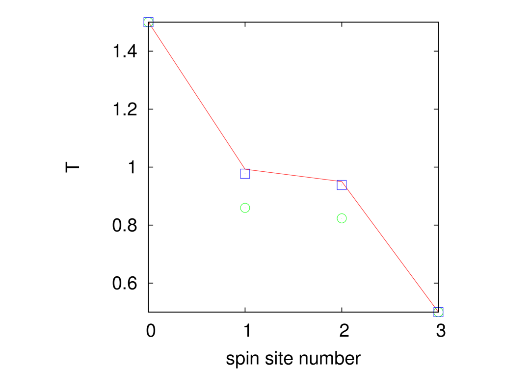
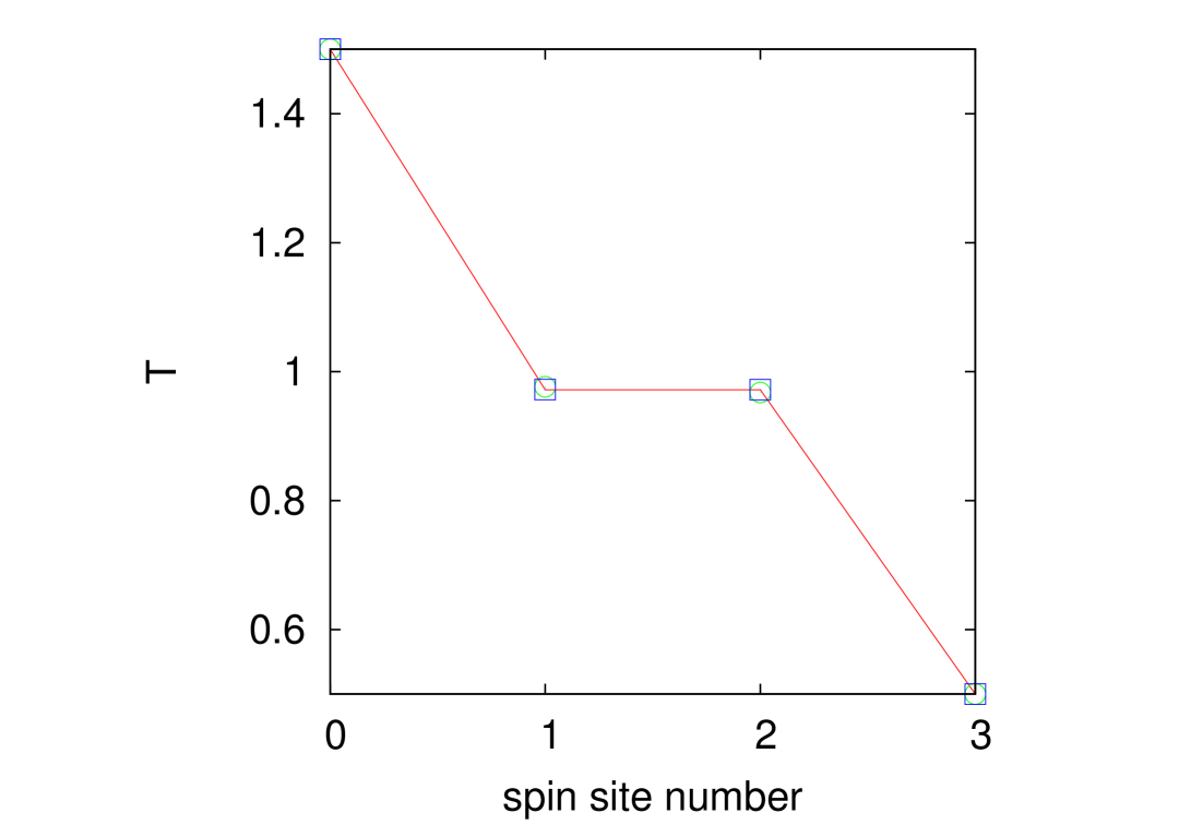
Figure 4: Temperature profiles for the two-spin tilted Ising model. The left and right figures show the results for $\theta=\pi/4$ and $\theta=\pi/2$ (transverse Ising model), respectively. The heat bath temperatures are $T_{L}=1.5$ and $T_{R}=0.5$, which are shown at the zeroth and third sites in the figure, respectively. The solid line shows the analytical results in Eqs. (111) and (112). The circles and squares are numerical results for $\lambda=0.1$ and $0.01$, respectively.

IV.3 $N$-spin case

Next we consider $N$-spin systems. Let us first consider the product of local equilibrium states:

$$\rho_{\rm PLE} \coloneqq \bigotimes_{m=1}^{N}\rho_{\rm LE}(\beta_{m}).$$ (115)

We write $\mathcal{L}_{1}$ as

$$\mathcal{L}_{1} = \sum_{l=1}^{N-1}\mathcal{L}_{{\rm I}(l,l+1)}+\mathcal{L}_{{\rm E}(1)}+\mathcal{L}_{{\rm E}(N)},$$ (116)

where $\mathcal{L}_{{\rm I}(l,l+1)}$ represents a local interaction,

$$\mathcal{L}_{{\rm I}(l,l+1)}\rho = -i[H_{{\rm I}(l,l+1)},\rho],$$ (117)

$$H_{{\rm I}(l,l+1)} \coloneqq \sum_{jk}\alpha_{jk}\sigma^{j}_{l}\otimes\sigma^{k}_{l+1},$$ (118)

and $\mathcal{L}_{{\rm E}(l)}$ represents the first-order contribution from a heat bath,

$$\mathcal{L}_{{\rm E}(l)}\rho = -i[H_{{\rm E}(l)},\rho],$$ (119)

$$H_{{\rm E}(l)} \coloneqq \alpha_{l}^{x}\sigma_{l}^{x}+\alpha_{l}^{y}\sigma_{l}^{y}+\alpha_{l}^{z}\sigma_{l}^{z}.$$ (120)

Then we have

$$\mathcal{P}_{0}\mathcal{L}_{\rm I(l,l+1)}\rho_{\rm PLE} = \frac{t_{l+1}-t_{l}}{4}\alpha_{+}\rho^{\rm B}_{l,l+1}\bigotimes_{m(\neq l,l+1)}\rho_{\rm LE}(\beta_{m})$$ (121)

and

$$\mathcal{P}_{0}\mathcal{L}_{{\rm E}(l)}\rho_{\rm PLE} = 0.$$ (122)

Since $\mathcal{P}_{0}\mathcal{L}_{1}\rho_{\rm PLE}\neq 0$, $\rho_{\rm PLE}$ is not the zeroth-order solution. Therefore we have to add some correction terms to $\rho_{\rm PLE}$ to obtain $\rho_{0}$. To cancel the two-body correlated term in Eq. (121), we have to add three-body correlated terms, but if we apply $\mathcal{P}_{0}\mathcal{L}_{1}$ to them, slightly different residual three-body terms appear. Then we have to add four-body correlated terms to cancel the three-body residual terms, which give new four-body residual terms, and so on. Thus, we obtain a BBGKY (Bogoliubov-Born-Green-Kirkwood-Yvon)-like hierarchy of equations, which is difficult to solve.

In this paper, we do not try to obtain $\rho_{0}$ explicitly. Instead, we consider local projections of the equation $\mathcal{P}_{0}\mathcal{L}_{1}\rho_{0}=0$. A one-site projection $\mathcal{P}_{(l)}$ traces out all spins except for that on the $l$th site. It gives no information, however, since $\rho_{\rm PLE}$ already satisfies

$$\mathcal{P}_{(l)}\mathcal{P}_{0}\mathcal{L}_{1}\rho_{\rm PLE} = 0.$$ (123)

Next we consider a two-site projection $\mathcal{P}_{(l,l+1)}$, which traces out all spins except for those at the $l$th and $(l+1)$th sites. Since

$$\mathcal{P}_{(l,l+1)}\mathcal{P}_{0}\mathcal{L}_{{\rm I}(m,m+1)}=0$$ (124)

if $l+1<m$ or $m+1<l$, only three interaction terms, $\mathcal{L}_{{\rm I}(l-1,l)}$, $\mathcal{L}_{{\rm I}(l,l+1)}$, and $\mathcal{L}_{{\rm I}(l+1,l+2)}$ matter when we consider $\mathcal{P}_{(l,l+1)}$. Hence, the equation to solve is

$$\mathcal{P}_{(l,l+1)}\mathcal{P}_{0}\left(\mathcal{L}_{{\rm I}(l-1,l)}+\mathcal{L}_{{\rm I}(l,l+1)}+\mathcal{L}_{{\rm I}(l+1,l+2)}\right)\rho_{0} = 0.$$ (125)

We write

$$\rho_{0} = \rho_{\rm PLE}+\rho_{a}.$$ (126)

Without loss of generality, we can assume that the additional term $\rho_{a}$ does not change the local state:

$$\mathcal{P}_{l}\rho_{0} = \rho_{\rm LE}(\beta_{l}).$$ (127)

Then the general form of $\rho_{a}$ that is relevant to Eq. (125) is

$$\rho_{a} = c^{\rm A}_{\overline{l-1},l,l+1}\sigma_{l-1}^{z}\rho^{\rm A}_{l,l+1}+c^{\rm B}_{\overline{l-1},l,l+1}\sigma_{l-1}^{z}\rho^{\rm B}_{l,l+1}+c^{\rm A}_{l-1,\overline{l},l+1}\sigma_{l}^{z}\rho^{\rm A}_{l-1,l+1}+c^{\rm B}_{l-1,\overline{l},l+1}\sigma_{l}^{z}\rho^{\rm B}_{l-1,l+1}$$ (128)

$$+c^{\rm A}_{l,\overline{l+1},l+2}\sigma_{l+1}^{z}\rho^{\rm A}_{l,l+2}+c^{\rm B}_{l,\overline{l+1},l+2}\sigma_{l+1}^{z}\rho^{\rm B}_{l,l+2}+c^{\rm A}_{l,l+1,\overline{l+2}}\rho^{\rm A}_{l,l+1}\sigma_{l+2}^{z}+c^{\rm B}_{l,l+1,\overline{l+2}}\rho^{\rm B}_{l,l+1}\sigma_{l+2}^{z}$$

$$+c^{\rm B}_{l,l+1}\rho^{\rm B}_{l,l+1}.$$

In the coefficients $c^{\alpha}_{p,q,r}$, the overline attached to a suffix shows the site where $\sigma^{z}$ is. We assume that, at a site whose state is unspecified, the state is $\sigma^{0}/2$, whose trace is unity. For example,

$$\sigma_{l-1}^{z}\rho^{\rm A}_{l,l+1} \coloneqq \sigma_{l-1}^{z}\rho^{\rm A}_{l,l+1}\bigotimes_{m(\neq l-1,l,l+1)}\frac{\sigma_{m}^{0}}{2}.$$ (129)

Substituting Eq. (128) into Eqs. (125) and (126), we obtain

$$\left\{\frac{t_{l+1}-t_{l}}{4}\alpha_{+}+4\alpha_{zz}(-c^{\rm A}_{\overline{l-1},l,l+1}+c^{\rm A}_{l,l+1,\overline{l+2}})+2\alpha_{+}(c^{\rm A}_{l-1,\overline{l},l+1}-c^{\rm A}_{l,\overline{l+1},l+2})\right\}\rho^{\rm B}_{l,l+1}$$

$$-2\left\{2\alpha_{zz}(-c^{\rm B}_{\overline{l-1},l,l+1}+c^{\rm B}_{l,l+1,\overline{l+2}})+\alpha_{+}(c^{\rm B}_{l-1,\overline{l},l+1}-c^{\rm B}_{l,\overline{l+1},l+2})\right\}\rho^{\rm A}_{l,l+1}$$

$$+2\alpha_{+}c^{\rm B}_{l,l+1}\rho_{l,l+1}^{C}=0,$$ (130)

where $\rho^{\rm C}_{l,m}\coloneqq\sigma^{0}_{l}\sigma^{z}_{m}-\sigma^{z}_{l}\sigma^{0}_{m}$. Hence,

$$(t_{l+1}-t_{l})\alpha_{+}+16\alpha_{zz}(-c^{\rm A}_{\overline{l-1},l,l+1}+c^{\rm A}_{l,l+1,\overline{l+2}})+8\alpha_{+}(c^{\rm A}_{l-1,\overline{l},l+1}-c^{\rm A}_{l,\overline{l+1},l+2}) = 0,$$ (131)

$$2\alpha_{zz}(-c^{\rm B}_{\overline{l-1},l,l+1}+c^{\rm B}_{l,l+1,\overline{l+2}})+\alpha_{+}(c^{\rm B}_{l-1,\overline{l},l+1}-c^{\rm B}_{l,\overline{l+1},l+2}) = 0,$$ (132)

$$c^{\rm B}_{l,l+1} = 0.$$ (133)

At the edges of the system, we have slightly different equations. For example, at the left edge ($l=1$), we have

$$\mathcal{P}_{(1,2)}\mathcal{P}_{0}(\mathcal{L}_{{\rm E}(1)}+\mathcal{L}_{{\rm I}(1,2)}+\mathcal{L}_{{\rm I}(2,3)})\rho_{0} = 0.$$ (134)

The general form of the relevant additional term is

$$\rho_{a} = c^{\rm A}_{1,\overline{2},3}\sigma_{2}^{z}\rho^{\rm A}_{1,3}+c^{\rm B}_{1,\overline{2},3}\sigma_{2}^{z}\rho^{\rm B}_{1,3}+c^{\rm A}_{1,2,\overline{3}}\rho^{\rm A}_{1,2}\sigma_{3}^{z}+c^{\rm B}_{1,2,\overline{3}}\rho^{\rm B}_{1,2}\sigma_{3}^{z}+c^{\rm A}_{1,2}\rho^{\rm A}_{1,2}+c^{\rm B}_{1,2}\rho^{\rm B}_{1,2}.$$ (135)

Substituting Eq. (135) into Eq. (134), we obtain

$$\left\{\frac{t_{2}-t_{1}}{4}\alpha_{+}+4\alpha_{zz}c^{\rm A}_{1,2,\overline{3}}-2\alpha_{+}c^{\rm A}_{1,\overline{2},3}-2\alpha_{1}^{z}c^{\rm A}_{1,2}\right\}\rho^{\rm B}_{1,2}$$

$$-2\left\{2\alpha_{zz}c^{\rm B}_{1,2,\overline{3}}-\alpha_{+}c^{\rm B}_{1,\overline{2},3}-\alpha_{1}^{z}c^{\rm B}_{1,2}\right\}\rho^{\rm A}_{1,2}$$

$$+2\alpha_{+}c^{\rm B}_{1,2}\rho_{1,2}^{C}=0,$$ (136)

Hence,

$$(t_{2}-t_{1})\alpha_{+}+16\alpha_{zz}c^{\rm A}_{1,2,\overline{3}}-8\alpha_{+}c^{\rm A}_{1,\overline{2},3}-8\alpha_{1}^{z}c^{\rm A}_{1,2} = 0,$$ (137)

$$2\alpha_{zz}c^{\rm B}_{1,2,\overline{3}}-\alpha_{+}c^{\rm B}_{1,\overline{2},3} = 0,$$ (138)

$$c^{\rm B}_{1,2} = 0.$$ (139)

In the same way, we obtain the following three equations at the right edge:

$$(t_{N}-t_{N-1})\alpha_{+}-16\alpha_{zz}c^{\rm A}_{\overline{N-2},N-1,N}+8\alpha_{+}c^{\rm A}_{N-2,\overline{N-1},N}+8\alpha_{N}^{z}c^{\rm A}_{N-1,N} = 0,$$ (140)

$$2\alpha_{zz}c^{\rm B}_{\overline{N-1},N-1,N}-\alpha_{+}c^{\rm B}_{N-2,\overline{N-1},N} = 0,$$ (141)

$$c^{\rm B}_{N-1,N} = 0.$$ (142)

Thus, we have obtained the following set of equations related to the temperature gradient:

$$t_{2}-t_{1} = \frac{8}{\alpha_{+}}(-2\alpha_{zz}c^{\rm A}_{1,2,\overline{3}}+\alpha_{+}c^{\rm A}_{1,\overline{2},3}+\alpha_{1}^{z}c^{\rm A}_{1,2}),$$ (143)

$$t_{3}-t_{2} = \frac{8}{\alpha_{+}}\left\{2\alpha_{zz}(c^{\rm A}_{\overline{1},2,3}-c^{\rm A}_{2,3,\overline{4}})+\alpha_{+}(-c^{\rm A}_{1,\overline{2},3}+c^{\rm A}_{2,\overline{3},4})\right\},$$ (144)

$$t_{4}-t_{3} = \frac{8}{\alpha_{+}}\left\{2\alpha_{zz}(c^{\rm A}_{\overline{2},3,4}-c^{\rm A}_{3,4,\overline{5}})+\alpha_{+}(-c^{\rm A}_{2,\overline{3},4}+c^{\rm A}_{3,\overline{4},5})\right\},$$ (145)

$$\vdots$$ (146)

$$t_{N-1}-t_{N-2} = \frac{8}{\alpha_{+}}\left\{2\alpha_{zz}(c^{\rm A}_{\overline{N-3},N-2,N-1}-c^{\rm A}_{N-2,N-1,\overline{N}})+\alpha_{+}(-c^{\rm A}_{N-3,\overline{N-2},N-1}+c^{\rm A}_{N-2,\overline{N-1},N})\right\},$$ (147)

$$t_{N}-t_{N-1} = \frac{8}{\alpha_{+}}(2\alpha_{zz}c^{\rm A}_{\overline{N-2},N-1,N}-\alpha_{+}c^{\rm A}_{N-2,\overline{N-1},N}-\alpha_{N}^{z}c^{\rm A}_{N-1,N}).$$ (148)

Summing these equations, all terms with $\alpha_{+}$ vanish and we obtain

$$t_{N}-t_{1} = \frac{8}{\alpha_{+}}\left\{2\alpha_{zz}\sum_{l=2}^{N-1}\left(c^{\rm A}_{\overline{l-1},l,l+1}-c^{\rm A}_{l-1,l,\overline{l+1}}\right)+\alpha_{1}^{z}c_{1,2}^{\rm A}-\alpha_{N}^{z}c_{N-1,N}^{\rm A}\right\}.$$ (149)

If we assume that the system-bath coupling has the same form as the spin-spin coupling as in Sect. IV.2, we have $\alpha_{1}^{z}=-\alpha_{zz}t_{\rm L}$ and $\alpha_{N}^{z}=-\alpha_{zz}t_{\rm R}$. Replacing the coefficients with the expectation values of the correlations, we obtain

$$t_{N}-t_{1} = \frac{\alpha_{zz}}{\alpha_{+}}\left\{\sum_{l=2}^{N-1}\left(\langle\sigma_{l-1}^{z}\rho^{\rm A}_{l,l+1}\rangle-\langle\rho^{\rm A}_{l-1,l}\sigma^{z}_{l+1}\rangle\right)-t_{\rm L}\langle\rho^{\rm A}_{1,2}\rangle+\langle\rho^{\rm A}_{N-1,N}\rangle t_{\rm R}\right\}.$$ (150)

This is our main result. The left-hand side (LHS) is related to the temperature difference between the two ends of the chain. Here, we see that $\alpha_{zz}\neq 0$ is necessary to form a nonzero temperature gradient. We can also see that the three-body correlations

$$\langle\sigma_{l-1}^{z}\rho^{\rm A}_{l,l+1}\rangle = \langle\sigma_{l-1}^{z}(\sigma^{x}_{l}\sigma^{x}_{l+1}+\sigma^{y}_{l}\sigma^{y}_{l+1})\rangle$$ (151)

and

$$\langle\rho^{\rm A}_{l-1,l}\sigma_{l+1}\rangle = \langle(\sigma^{x}_{l-1}\sigma^{x}_{l}+\sigma^{y}_{l-1}\sigma^{y}_{l})\sigma_{l+1}^{z}\rangle$$ (152)

play essential roles in forming the temperature gradient. Note that the two-body correlation terms related to the heat baths also have similar forms since $t_{l}=-\langle\sigma_{l}\rangle$.

In Fig. 5 we show numerically obtained temperature profiles for the tilted Ising model with $N=6$. We see that the temperature gradient is nonzero for $\theta=\pi/4$, where $\alpha_{zz}\neq 0$, while it vanishes for $\theta=\pi/2$, where $\alpha_{zz}=0$, as expected from Eq. (150). In the case with $\theta=\pi/4$, the numerical results agree with the weak-coupling limit for $\lambda=0.01$, with relative errors of order $10^{-2}$. The convergence is as fast as for the two-spin case. For $\theta=\pi/2$, the convergence is much faster, which is also the same as in the two-spin case.

In Fig. 6 we show numerical results for the LHS and the right-hand side (RHS) of Eq. (150). We see that both sides converge to the same value in the weak-coupling limit, although the convergence is slightly slower than that for the temperature.

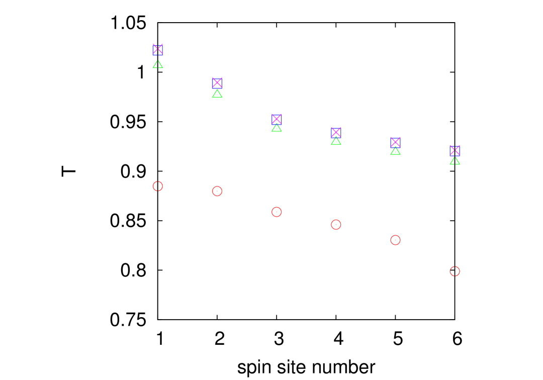
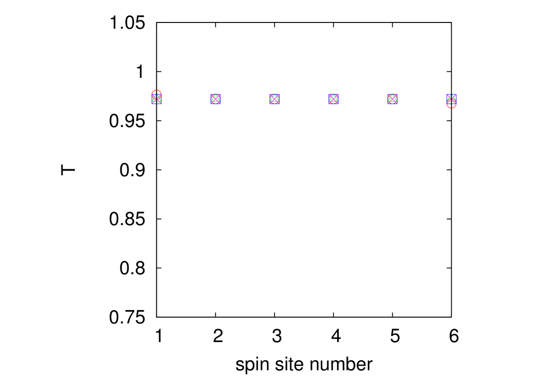
Figure 5: Temperature profiles for the tilted Ising model with $N=6$. The left and right figures correspond to $\theta=\pi/4$ and $\theta=\pi/2$, respectively. The circles, triangles, squares, and crosses show the numerical results for $\lambda=10^{-1},10^{-2},10^{-3}$, and $10^{-4}$, respectively. The other parameters, which are not written explicitly here, are the same as those for the two-spin case in Fig. 4.

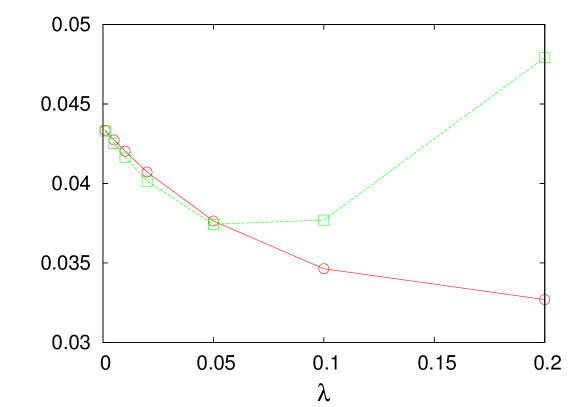
Figure 6: Numerical results for the LHS (circles) and RHS (squares) of Eq. (150). The coupling parameter is taken as $\lambda=0.001,0.005,0.01,0.02,0.05,0.1$, and $0.2$.

V Summary

We considered NESSs in weakly coupled one-dimensional quantum spin-1/2 chains. The spin-spin coupling and system-bath coupling were assumed to be of the same order. We derived the QME for this case, in which the heat bath superoperator becomes local. We developed a perturbative expansion for the stationary solution of the QME. For the two-spin case, we gave an explicit example in which the zeroth-order solution has a nonzero temperature gradient. For the general $N$-spin case, we showed that $\alpha_{zz}\neq 0$ is necessary to obtain a nonzero temperature gradient. We also showed that some three-body correlations are essential for the formation of a temperature gradient.

Appendix A Proof of Eq. (44)

Let us denote a matrix element of $H_{1}$ as

$$d_{n,k,m,l}\coloneqq\langle E_{n,k}|H_{1}|E_{m,l}\rangle.$$ (153)

It satisfies

$$d_{n,k,m,l} = d_{m,l,n,k}^{*}.$$ (154)

We apply $\mathcal{L}_{1}\left(Q_{0}\mathcal{L}_{0}Q_{0}\right)^{-1}\mathcal{L}_{1}\mathcal{P}_{1}$ to a basis element $|E_{n,k}\rangle\langle E_{n,k}|$ in $\mathtt{Im\,}\mathcal{P}_{1}$. Then we obtain

$$\mathcal{L}_{1}\left(\mathcal{Q}_{0}\mathcal{L}_{0}\mathcal{Q}_{0}\right)^{-1}\mathcal{L}_{1}|E_{n,k}\rangle\langle E_{n,k}|$$ (155)

$$= \frac{1}{i\hbar}\sum_{p,q}\sum_{m(\neq n),l}\frac{1}{E_{m}-E_{n}}\left\{|E_{p,q}\rangle d_{p,q,m,l}d_{m,l,n,k}\langle E_{n,k}|-|E_{m,l}\rangle d_{m,l,n,k}d_{n,k,p,q}\langle E_{p,q}|\right.$$

$$\left.+|E_{p,q}\rangle d_{p,q,n,k}d_{n,k,m,l}\langle E_{m,l}|-|E_{n,k}\rangle d_{n,k,m,l}d_{m,l,p,q}\langle E_{p,q}|\right\}.$$

Applying $\mathcal{P}_{1}$ to the above equation, we have

$$\mathcal{P}_{1}\mathcal{L}_{1}\left(\mathcal{Q}_{0}\mathcal{L}_{0}\mathcal{Q}_{0}\right)^{-1}\mathcal{L}_{1}|E_{n,k}\rangle\langle E_{n,k}|$$ (156)

$$= \frac{1}{i\hbar}\sum_{m(\neq n),l}\frac{1}{E_{m}-E_{n}}\left\{|E_{n,k}\rangle|d_{m,l,n,k}|^{2}\langle E_{n,k}|-|E_{m,l}\rangle|d_{m,l,n,k}|^{2}\langle E_{m,l}|\right.$$

$$\left.+|E_{m,l}\rangle|d_{m,l,n,k}|^{2}\langle E_{m,l}|-|E_{n,k}\rangle|d_{m,l,n,k}|^{2}\langle E_{n,k}|\right\}$$

$$= 0.$$ (157)

Hence, Eq. (44) is proven.

Appendix B Two-spin tilted Ising model

In this appendix, we show the details of the calculation of the zeroth-order solution for the two-spin tilted Ising model.

First we consider a single bath and assume spin-bath coupling of the form $\sigma^{z^{\prime}}\otimes\sigma^{z^{\prime}}$, where

$$\sigma^{z^{\prime}} = \sigma^{z}\cos\theta-\sigma^{x}\sin\theta.$$ (158)

Then the heat bath superoperator becomes

$$\mathcal{D}\rho=-\left([\sigma^{z^{\prime}},S\rho]+h.c.\right),$$ (159)

where

$$S = \left(\begin{array}[]{cc}\Xi_{\beta}(0)\cos\theta&-\Xi_{\beta}(2h)\sin\theta\\ -\Xi_{\beta}(-2h)\sin\theta&-\Xi_{\beta}(0)\cos\theta\end{array}\right),$$ (162)

$$\Xi_{\beta}(\omega) = \int_{0}^{\infty}dte^{-i\omega t}\Phi_{\beta}(t),$$ (163)

$$\Phi_{\beta}(t) = \langle\Delta\sigma^{z^{\prime}}(t)\Delta\sigma^{z^{\prime}}\rangle_{\beta}.$$ (164)

Here, $\langle\cdot\rangle_{\beta}$ represents the equilibrium average in the heat bath at the inverse temperature $\beta$. We removed suffices $j,l$ from $\Xi$ and $\Phi$ since the system-bath coupling is represented by a single term, and use the subscript $\beta$ to show the inverse temperature of the heat bath explicitly. Note that we take $\hbar=1$ here.

$\Xi_{\beta}$ can be written as

$$\Xi_{\beta}(\omega) = \frac{1}{2}\left\{\tilde{\Phi}_{\beta}(\omega)+i\Psi_{\beta}(\omega)\right\},$$ (165)

where the real part is represented by the Fourier transform of $\Phi_{\beta}(t)$:

$$\tilde{\Phi}_{\beta}(\omega) = \int_{-\infty}^{\infty}dte^{-i\omega t}\Phi_{\beta}(t).$$ (166)

It satisfies the KMS (Kubo-Martin-Schwinger) condition kubo

$$\tilde{\Phi}_{\beta}(-\omega) = \tilde{\Phi}_{\beta}(\omega)e^{\beta\omega}$$ (167)

and $\tilde{\Phi}(\omega)\geq 0$. We ignore the imaginary part $\Psi_{\beta}$ because usually it does not give a significant contribution.saito2

Then

$$S = \frac{1}{2}\left\{b\sigma_{z}-a(\sigma_{x}-it\sigma_{y})\right\},$$ (168)

where

$$a = \frac{\tilde{\Phi}_{\beta}(2h)+\tilde{\Phi}_{\beta}(-2h)}{2}\sin\theta,$$ (169)

$$b = \tilde{\Phi}_{\beta}(0)\cos\theta,$$ (170)

$$t = \tanh(\beta h).$$ (171)

Thus, we have

$$\mathcal{D}\sigma_{0} = -2at(\sigma_{x}\cos\theta+\sigma_{z}\sin\theta),$$ (172)

$$\mathcal{D}\sigma_{x} = -2b(\sigma_{x}\cos\theta-\sigma_{z}\sin\theta),$$ (173)

$$\mathcal{D}\sigma_{y} = -2(b\cos\theta+a\sin\theta)\sigma_{y},$$ (174)

$$\mathcal{D}\sigma_{z} = -2a(\sigma_{x}\cos\theta+\sigma_{z}\sin\theta).$$ (175)

Next we apply $\mathcal{P}_{1}\mathcal{L}_{2}=\mathcal{P}_{1}(\mathcal{D}_{\rm L}+\mathcal{D}_{\rm R})$ to Eq. (103). Then we obtain

$$\mathcal{P}_{1}\mathcal{L}_{2}\rho_{0}$$ (177)

$$= -\frac{\sin\theta}{2}\left\{a_{L}(t_{1}-t_{\rm L})t_{2}+a_{R}(t_{2}-t_{\rm R})t_{1}+4g(a_{L}+a_{R})\right\}\sigma^{zz}$$

$$+\frac{\sin\theta}{4}\left\{a_{L}(t_{1}-t_{\rm L})+a_{R}(t_{2}-t_{\rm R})\right\}(\sigma^{0z}+\sigma^{z0})$$

$$+\frac{1}{8(1+\gamma^{2})}\left[2\sin\theta\left\{a_{R}(t_{2}-t_{\rm R})-a_{L}(t_{1}-t_{\rm L})\right\}\right.$$

$$\left.+\gamma^{2}(t_{2}-t_{1})\left\{2(b_{L}+b_{R})\cos\theta+(a_{L}+a_{R})\sin\theta\right\}\right]\rho^{C^{\prime}},$$

with obvious notations. Since in this case

$$\overline{H}_{SB} = \langle\sigma^{z^{\prime}}\rangle_{\beta_{L}}\sigma_{1}^{z^{\prime}}\otimes\sigma_{2}^{0}+\sigma_{1}^{0}\otimes\sigma_{2}^{z^{\prime}}\langle\sigma^{z^{\prime}}\rangle_{\beta_{R}}$$ (178)

$$= -\cos\theta\left(t_{\rm L}\sigma_{1}^{z^{\prime}}\otimes\sigma_{2}^{0}+t_{\rm R}\sigma_{1}^{0}\otimes\sigma_{2}^{z^{\prime}}\right),$$ (179)

we have

$$\Delta\alpha_{z}=-(t_{\rm L}-t_{\rm R})\cos^{2}\theta$$ (180)

and

$$\gamma=\frac{\alpha_{xx}+\alpha_{yy}}{\Delta\alpha_{z}}=-\frac{\sin^{2}\theta}{(t_{\rm L}-t_{\rm R})\cos^{2}\theta}.$$ (181)

We can determine $t_{1},t_{2}$, and $g$ by solving the following three equations:

$$a_{L}(t_{1}-t_{\rm L})t_{2}+a_{R}(t_{2}-t_{\rm R})t_{1}+4g(a_{L}+a_{R}) = 0,$$ (182)

$$a_{L}(t_{1}-t_{\rm L})+a_{R}(t_{2}-t_{\rm R}) = 0,$$ (183)

$$2\sin\theta\left\{a_{\rm R}(t_{2}-t_{\rm R})-a_{\rm L}(t_{1}-t_{\rm L})\right\}+\gamma^{2}(t_{2}-t_{1})\left\{2(b_{\rm L}+b_{\rm R})\cos\theta+(a_{\rm L}+a_{\rm R})\sin\theta\right\}=0.$$ (184)

When $t_{\rm L}-t_{\rm R}\ll 1$, $a_{\rm L}\simeq a_{\rm R}$ and $b_{\rm L}\simeq b_{\rm R}$. Hence, we obtain

$$t_{1} = \frac{t_{\rm L}+t_{\rm R}}{2}+\frac{K}{2}(t_{\rm L}-t_{\rm R}),$$ (185)

$$t_{2} = \frac{t_{\rm L}+t_{\rm R}}{2}-\frac{K}{2}(t_{\rm L}-t_{\rm R}),$$ (186)

$$g = -\frac{K(1-K)}{16}(t_{\rm L}-t_{\rm R})^{2},$$ (187)

ignoring higher-order terms with respect to $t_{\rm L}-t_{\rm R}$. Here,

$$K \coloneqq \frac{c(t_{\rm L}-t_{\rm R})^{2}\cos^{4}\theta}{c(t_{\rm L}-t_{\rm R})^{2}\cos^{4}\theta+\sin^{2}\theta(2d\cos^{2}\theta+c\sin^{2}\theta)}$$ (188)

and

$$c \coloneqq \frac{c_{\rm L}+c_{\rm R}}{2},$$ (189)

$$d \coloneqq \frac{d_{\rm L}+d_{\rm R}}{2},$$ (190)

where

$$c_{\alpha} \coloneqq \frac{\tilde{\Phi}_{\beta_{\alpha}}(2h)+\tilde{\Phi}_{\beta_{\alpha}}(-2h)}{2},$$ (191)

$$d_{\alpha} \coloneqq \tilde{\Phi}_{\beta_{\alpha}}(0),$$ (192)

and $\alpha={\rm L},{\rm R}$. Note that $a_{\alpha}=c_{\alpha}\sin\theta$ and $b_{\alpha}=d_{\alpha}\cos\theta$. Since $c,d\geq 0$, $K$ satisfies $0\leq K\leq 1$. $K=0$ holds for $\theta=\pi/2$ (horizontal magnetic field), and $K=1$ for $\theta=0$ (vertical magnetic field).

References

• (1) S. Lepri, R. Livi, and A. Politi, Phys. Rep. 377, 1 (2003).
• (2) T. Prosen and M. Žnidarič, J. Stat. Mech. P02035 (2009).
• (3) M. Michel, O. Hess, H. Wichterich, and J. Gemmer, Phys. Rev. B 77, 104303 (2008).
• (4) J. Wu and M. Berciu, Phys. Rev. B 83, 214416 (2011).
• (5) J. J. Mendoza-Arenas, S. Al-Assam, S. R. Clark, and D. Jaksch, J. Stat. Mech. P07007 (2013).
• (6) T. Yuge and A. Sugita, J. Phys. Soc. Jpn. 84, 014001 (2014).
• (7) A. Sugita, Proc. Recent Advances in the Physics of Low-Dimensional Nanoscale Systems, arXiv:1203.3817.
• (8) R. Kubo, M. Toda, and N. Hashitsume, Statistical Physics II: Nonequilibrium Statistical Mechanics (Springer, Berlin, 1991) 2nd ed.
• (9) H.-P. Breuer and F. Petruccione, The Theory of Open Quantum Systems (Oxford University Press, London, 2002).
• (10) A. Sugita, RIMS Kokyuroku 1507, 147 (2006) [in Japanese]; Nonlinear Phenom. Complex Syst. 10, 192 (2007).
• (11) S. Sugiura and A. Shimizu, Phys. Rev. Lett. 108, 240401 (2012); Phys. Rev. Lett. 111, 010401 (2013).
• (12) K. Saito, S. Takesue, and S. Miyashita, Phys. Rev. E 54, 2404 (1996).
• (13) K. Saito, S. Takesue, and S. Miyashita, Phys. Rev. E 61, 2397 (2000).