Modeling and simulation of thermally actuated bilayer plates

Abstract.

We present a mathematical model of polymer bilayers that undergo large bending deformations when actuated by non-mechanical stimuli such as thermal effects. The simple model captures a large class of nonlinear bending effects and can be discretized with standard plate elements. We devise a fully practical iterative scheme and apply it to the simulation of folding of several practically useful compliant structures comprising of thin elastic layers.

1. Introduction

Bilayer polymers are appealing for the development of autonomous lightweight foldable structures, such as drug delivery vesicles, flexible constructions for soft robots, self-deployable sun sails in spacecraft, and morphing structures, since they can be manufactured into various shapes with tunable material properties for each layer. A characteristic feature is that they can undergo controlled large deformations via relatively small external stimuli. Bilayers having two polymeric layers with different thermo-responsive and swelling characteristics have been shown capable of forming various practically useful folding shapes [28, 6, 2]. Different expansion/contraction characteristics of the two layers when exposed to temperature changes or solvent diffusions lead to out of plane rotations and curvature changes of the bilayers which trigger folding, cf. Fig. 1. When the two layers have significantly different expansion/contraction behaviors, often characterized by the coefficient of thermal or moisture expansion, folding can be achieved with relatively smaller stimuli. However, high contrast in mechanical properties, i.e., elastic modulus, between the two layers can induce high stress discontinuities between the layers, leading to delamination. Another mechanism for folding and bending of bilayers can be achieved by integrating two electro-active polymers with the opposite directions of through-thickness poling axes and when the bilayers are subjected to electric potential through the thickness one layer would expand while the other would contract [31, 30, 21]. One of the advantages of combining two polymers with different responsive characteristics with regard to their non-mechanical performances is that the mechanical properties of polymers do not vary significantly, e.g., extensional elastic moduli of various polymers are typically between $0.5-5.0\,{\rm GPa}$, which can minimize stress discontinuities at the interfaces between the two layers and thus can avoid failure due to delamination. Alternatively, bilayers can be formed by combining two different types of materials, i.e., metal- or ceramic-polymer, which have significant differences in their mechanical and non-mechanical properties [25, 14].

\begin{picture}(4951.0,503.0)(-52.0,53.0)\end{picture}

Figure 1. Schematic description of a thermally actuated bilayer: heat diffusion starts from the sides into polymer layers that compress and expand and which are placed between two insulating layers.

We are specifically interested in bilayers comprising of two polymeric layers that can undergo large deformations when exposed to non-mechanical stimuli, such as temperature changes or fluid sorption. Due to the slender nature of the bilayers, large deformations are mainly governed by rotations while the strains in the bilayer are relatively small [26, 30], thereby leading to negligible stretching and transverse shear effects. Furthermore, the mid-surface of the bilayer plate is considered to be inextensible and non-shearable, thereby leaving bending as a chief mechanism for shape deformation. These basic mechanical assumptions lead to a reduced Kirchhoff plate model for the deformation with a preferred curvature tensor and an isometry constraint. The former encodes the mismatch between bilayers while the latter reflects the property that distances among points on the mid surface do not change with shape deformation. In addition, we ignore inertial effects and assume a quasi-static evolution of the plate.

The bilayer plate is driven by heat conduction or fluid sorption. We model this diffusion process with a linear Fourier heat conduction or Fickian diffusion law. Since the deformation is an isometry, the diffusion equation is insensitive to the plate deformation, whereas the temperature affects the mismatch between lower and upper layers of the plate. In several experimental studies, the bilayers are insulated on top and bottom and subjected to uniform environmental conditions on their sides, e.g., at dry conditions the bilayer is immersed in fluid or from curing at high temperature the bilayer is cooled down to room temperature or vice versa. In such situations, the entire polymers will be at uniform temperature or will have uniform fluid content at the steady state and the diffusion process occurs from the boundaries of the bilayers. We model this with homogeneous Neumann boundary condition on top and bottom of the plate, and either Neumann or Robin boundary conditions on the sides of the plate. We derive a reduce diffusion model that accounts for these effects.

Our investigations are motivated by lab experiments reporting problems in the controlled fabrication of nanotubes, cf. [28, 35, 33, 34]. In particular, rectangular bilayer plates occasionally start bending from the corners leading to formation of so-called dog-ears, thus failing to attain the desired cylindrical shape. Our mathematical model and corresponding simulations indicate that this may be attributed to too rapid changes in the environment that yield high concentrations of the diffusing quantity at the corners of the bilayer. Moreover, we present computational experiments resembling origami structures such as self-assembling cube [29, 13] and deployable airfoil [17], as well as particle encapsulation which is of interest in drug targeting [27]. Although additional effects become relevant at the nanoscale, see e.g. [32], our computational model could be utilized as a simple tool to explore and predict conditions and configurations that enable a controlled production of nanoscale and microscale devices. The method is advantageous with respect to direct simulation of full three-dimensional thermo-elasticity in terms of simplicity of implementation, efficiency, performance, and flexibility.

Our simple two-dimensional model is thus able to capture the principal mechanical and thermal effects responsible for large deformations observed in lab experiments of thermally actuated bilayer plates. This suffices for the aforementioned applications. In fact, the present model and analyses can help designers in simulating desired shape changes and determining external stimuli to be prescribed prior to fabricating flexible bilayer systems. We refer the reader to [1, 6, 15, 18, 23, 24, 25, 27, 28, 36] for further discussion on the applications. In contrast, a three-dimensional model capturing strong swelling effects and which leads to a two-way coupling of the diffusion and deformation processes has been investigated in [20].

Most of available studies with regards to folding of polymeric composite structures have been on fabrication and experiments. The mathematical description and numerical treatment of large bending deformations of elastic solids has recently undergone some important development. Dimensionally reduced models have been derived rigorously from three-dimensional hyperelasticity [10, 21] and numerical methods capable of approximating large rotations correctly have been devised and analyzed in [3, 4, 5]. In this work we extend the approach from [5] by including temperature dependence in the preferred curvature tensor. The mechanical part consists of a nonlinear Kirchhoff model for which we devise a finite element discretization based on standard plate elements. The heat equation decouples from the mechanical equation due to the inextensibility of the plate and we approximate it with standard finite element methods together with the backward Euler time stepping algorithm. The proposed iterative numerical method for the coupled system is roughly ten times faster than the one used in [5].

The outline of this article is as follows. In Section 2 we introduce the thermo-mechanical mathematical model and describe its dimension reduction. Corresponding partial differential equations are formulated in Section 3. We then present in Section 4 the temporal and spatial discretization of the nonlinear and constrained system composed of second order diffusion and fourth order bending equations. We report several intruiguing and practically useful numerical experiments in Section 5.

2. Mathematical model

2.1. Hyperelastic materials

We model polymers as isotropic and elastic materials. According to St. Venant–Kirchhoff description, the mechanical behavior of the system is governed by a hyperelastic stored energy density

$$W(E):=\mu|E|^{2}+\frac{\lambda}{2}({\rm tr}E)^{2},$$

where $E:=F^{\rotatebox[origin={c}]{180.0}{\footnotesize$\perp$}}F-I$ is the Green–Lagrange strain tensor related to the deformation gradient $F$, and $\lambda,\mu$ are the (first and second) Lamé constants [19]; hereafter we let $|E|^{2}=E:E$ be the square of the Frobenius norm of $E$ and ${\rm tr}E=E:I$ be the trace of $E$. As strain tensor we use the temperature dependent quantity $E_{\Theta}:=F^{\rotatebox[origin={c}]{180.0}{\footnotesize$\perp$}}F-(1+\alpha\Theta)I\in\mathbb{R}^{3\times 3}$ which generalizes the Green–Lagrange strain tensor. Here $\alpha,\Theta$ are the thermal expansion coefficient and temperature change. Therefore, a simple calculation yields

$$W(E_{\Theta})=W(E)-(2\mu+3\lambda)\alpha\Theta{\rm tr}E+c_{\Theta}$$

with $c_{\Theta}:=(3\mu+\frac{9}{2}\lambda)\alpha^{2}\Theta^{2}$. We note that the elastic material constants $\lambda,\mu$ can also change with temperature or fluid concentration. We simplify the model further upon realizing that $({\rm tr}E)^{2}\leq 3|E|^{2}$, whence

$$\mu|E_{\Theta}|^{2}\leq W(E_{\Theta})\leq\big{(}\mu+\frac{3\lambda}{2}\big{)}|E_{\Theta}|^{2}.$$

This equivalence motivates our choice of energy

(1) $$W_{\Theta}(F):=\frac{\mu}{4}|E_{\Theta}|^{2}=\frac{\mu}{4}\big{|}F^{\rotatebox[origin={c}]{180.0}{\footnotesize$\perp$}}F-(1+\alpha\Theta)I\big{|}^{2}.$$

which in turn allows us to follow the arguments of [5] for the formal dimension reduction of the plate model. A rigorous derivation for more general material models including the above St. Venant–Kirchhoff material can be found in [21] which leads to the same dimensionally reduced model up to a different prefactor in the energy density. For further details on admissible energies and relaxation effects of the dimension reduction, we refer the reader to [11, 10, 20, 21]. We remark that a more general, nonlinear dependence of the strain tensor on temperature can be used; for our experiments a linear relation turned out to be sufficient.

2.2. Bilayer configuration and evolution hypotheses

We consider the following configuration below. We let $\omega\subset\mathbb{R}^{2}$ be the flat parametric domain, $\delta>0$ be the thickness of the plate, and $\omega_{\delta}:=\omega\times(-\delta/2,\delta/2)$ be the plate in the undeformed configuration. We let $\mathbf{x}:=(\mathbf{x}^{\prime},x_{3})\in\omega_{\delta}$ denote a generic point and $t\in(0,\infty)$ time. We further indicate with $\mathbf{u}(\cdot,t):\omega_{\delta}\to\mathbb{R}^{3}$ the deformation of the plate and $\gamma_{\delta}(t)=\mathbf{u}(\cdot,t)(\omega_{\delta})$ the deformed configuration of the plate at time $t$.

For the evolution model considered below we assume that inertial effects are insignificant and that no mechanical dissipation occurs so that the plate immediately adjusts to temperature changes. This yields a dynamics driven by temperature, which mathematically entails that $\Theta$ solves a suitable diffusion equation on the flexible surface and $\mathbf{u}(\cdot,t)$ is a minimizer of an elastic energy associated with the density $W_{\Theta}(\nabla\mathbf{u}(\cdot,t))$. Due to the assumptions of thermal insulation of the bilayer top and bottom and of mid-surface inextensibility, it turns out that the diffusion equation decouples from the deformation equation. We examine these two models below and outline reduced models for the vanishing thickness limit $\delta\to 0$.

2.3. Reduced bilayer plate model

We adjust the simplified energy (1) for hyperelastic materials to model thin bilayers and derive effective energies describing large deformations. In particular, we consider two layers of materials glued on top of each other with different thermal material constants such as the thermal expansion coefficients. We assume that one material expands and the other compresses above a critical temperature, which we assume to be zero for simplicity. Therefore, we consider (1) with $F=\nabla\mathbf{u}$

$$W_{\Theta}(\nabla\mathbf{u},\mathbf{x},t)=\frac{\mu(\mathbf{x})}{4}\Big{|}\nabla\mathbf{u}^{\rotatebox[origin={c}]{180.0}{\footnotesize$\perp$}}\nabla\mathbf{u}-(1+\alpha(\mathbf{x})\Theta(\mathbf{x},t))I\Big{|}^{2},$$

where the coefficients $\alpha(\mathbf{x}),\mu(\mathbf{x})$ jump across $x_{3}=0$

$$\alpha(\mathbf{x}):=\begin{cases}+\alpha&\mbox{for }x_{3}>0,\\ -\alpha&\mbox{for }x_{3}<0,\end{cases}\qquad\mu(\mathbf{x}):=\begin{cases}\mu^{+}(x^{\prime})&\mbox{for }x_{3}>0,\\ \mu^{-}(x^{\prime})&\mbox{for }x_{3}<0.\end{cases}$$

We follow [11, 22, 5] to identify a dimensionally reduced model corresponding to the limit $\delta\to 0$. Formally, this is based on the Kirchhoff assumption that the actual deformation $\mathbf{u}$, subject to given forces and boundary conditions can be, up to higher order contributions, represented as

(2) $$\mathbf{u}(\mathbf{x}^{\prime},x_{3},t)=\mathbf{y}(\mathbf{x}^{\prime},t)+x_{3}\mathbf{b}(\mathbf{x}^{\prime},t)$$

with a mapping $\mathbf{y}:\omega\times(0,\infty)\to\mathbb{R}^{3}$ that describes the deformation of the midplane $\omega\times\{0\}$ and a vector field $\mathbf{b}:\omega\times(0,\infty)\to\mathbb{R}^{3}$ that is normal to the deformed midplane $\gamma(t)=\mathbf{y}(\omega,t)$. This means that fibers perpendicular to $\omega$ in the undeformed configuration remain normal to the mid-surface $\gamma(t)$ in the deformed configuration. For ease of presentation we do not write the argument $t$ explicitly in the remainder of this subsection. Inserting the corresponding deformation gradient

$$\nabla\mathbf{u}(\mathbf{x})=[\nabla^{\prime}\mathbf{y}(\mathbf{x}^{\prime}),\mathbf{b}(\mathbf{x}^{\prime})]+x_{3}[\nabla^{\prime}\mathbf{b}(\mathbf{x}^{\prime}),0]$$

into the scaled elastic energy functional

$$I_{\Theta}[\mathbf{u}]=\frac{1}{\delta^{3}}\int_{\omega_{\delta}}W_{\Theta}(\nabla\mathbf{u},\cdot)$$

leads to

$$\begin{split}I_{\Theta}[\mathbf{u}]=\frac{1}{\delta^{3}}\int_{\omega}\int_{-\delta/2}^{\delta/2}\frac{\mu}{4}\Bigg{\{}\Bigg{|}&\begin{bmatrix}(\nabla^{\prime}\mathbf{y})^{\rotatebox[origin={c}]{180.0}{\footnotesize$\perp$}}\nabla\mathbf{y}-(1\pm\alpha\Theta)I_{2}&0\\ 0&|\mathbf{b}|^{2}-(1\pm\alpha\Theta)\end{bmatrix}\\ +x_{3}&\begin{bmatrix}(\nabla^{\prime}\mathbf{b})^{\rotatebox[origin={c}]{180.0}{\footnotesize$\perp$}}\nabla^{\prime}\mathbf{y}+(\nabla^{\prime}\mathbf{y})^{\rotatebox[origin={c}]{180.0}{\footnotesize$\perp$}}\nabla^{\prime}\mathbf{b}&(\nabla^{\prime}\mathbf{b})^{\rotatebox[origin={c}]{180.0}{\footnotesize$\perp$}}\mathbf{b}\\ \mathbf{b}^{\rotatebox[origin={c}]{180.0}{\footnotesize$\perp$}}\nabla^{\prime}\mathbf{b}&0\end{bmatrix}\\ +x_{3}^{2}&\begin{bmatrix}(\nabla^{\prime}\mathbf{b})^{\rotatebox[origin={c}]{180.0}{\footnotesize$\perp$}}\nabla^{\prime}\mathbf{b}&0\\ 0&0\end{bmatrix}\Bigg{|}^{2}\Bigg{\}}.\end{split}$$

The scaling of the elastic energy by $\delta^{-3}$ corresponds to deformations that describe a bending behavior of the thin plate and is crucial for identifying limiting equations. We assume that $I_{\Theta}[\mathbf{u}]$ remains bounded as $\delta\to 0$, carry out the integration in $x_{3}$ direction, and deduce necessary scaling properties of terms arising in the energy functional; details can be found in [5]. The first necessary condition to have a finite limit as $\delta\to 0$ is that $\mathbf{b}$ has length $|\mathbf{b}|=1\pm\alpha\Theta$ in the upper and lower layers. Assuming that $\alpha/\delta$ is finite, which is explained below, shows that for $\delta\to 0$ we have that $\mathbf{b}$ equals the unit normal ${\boldsymbol{\nu}}$ to the deformed midplane $\gamma$ and that $(\nabla^{\prime}\mathbf{b})^{\rotatebox[origin={c}]{180.0}{\footnotesize$\perp$}}\mathbf{b}=0$. Let $G$ and $H$ be the first and second fundamental forms of $\gamma$, i.e., the symmetric matrices

$$G=(\nabla^{\prime}\mathbf{y})^{\rotatebox[origin={c}]{180.0}{\footnotesize$\perp$}}\nabla^{\prime}\mathbf{y},\quad H=-(\nabla^{\prime}{\boldsymbol{\nu}})^{\rotatebox[origin={c}]{180.0}{\footnotesize$\perp$}}\nabla^{\prime}\mathbf{y}.$$

Then we find the second necessary condition $G=I_{2}$ for a finite limit $\delta\to 0$,

$$[\nabla^{\prime}\mathbf{y}]^{T}\nabla^{\prime}\mathbf{y}=I_{2},$$

i.e., $\mathbf{y}:\omega\to\mathbb{R}^{3}$ defines an isometric deformation of the midplane $\omega$. With this we derive the central identity

$$\delta^{-3}\int_{-\delta/2}^{\delta/2}\frac{\mu}{4}|2x_{3}H\mp\alpha\Theta I_{2}|^{2}=\frac{\overline{\mu}}{12}\Big{(}|H-\overline{\alpha}\theta I_{2}|^{2}-\frac{4}{3}\overline{\alpha}^{2}\theta^{2}\Big{)},$$

in which $\overline{\mu}$ is the average of $\mu(\cdot,\pm x_{3})$, $\theta(\mathbf{x}^{\prime})=\Theta(\mathbf{x}^{\prime},0)$ is the effective temperature that obeys a reduced diffusion equation discussed below, and $\overline{\alpha}$ is the effective thermal expansion coefficient per unit thickness given by

(3) $$\overline{\alpha}:=\lim_{\delta\to 0}\frac{3\,\alpha}{\delta}.$$

Note that $\overline{\alpha}\theta$ has the unit of a curvature, i.e. $\text{\,}{\mathrm{m}}^{-1}$.

We thus infer that the reduced energy functional takes the form

(4) $$E[\mathbf{y}]=\frac{1}{12}\int_{\omega}\overline{\mu}\big{|}H-\overline{\alpha}\theta I_{2}\big{|}^{2},$$

up to constant terms that we ignore from now on. Assuming that $\alpha$ is comparable with the plate thickness is necessary to avoid delamination and obtain a total bending effect of the thin bilayer plate resulting from a compressive and expansive behavior of the individual layers. This also shows that small material differences can lead to large deformations.

2.4. Reduced diffusion model

As in the mechanical part we allow the two different materials in the upper and lower layers of the plate to possess different physical constants, namely heat capacities $\sigma^{\pm}$ and conductivities $\kappa^{\pm}$. We define

(5) $$\overline{\sigma}:=\frac{1}{2}(\sigma^{+}+\sigma^{-}),\quad\overline{\kappa}:=\frac{1}{2}(\kappa^{+}+\kappa^{-})$$

to be their mean values in the transversal direction. We make the key simplifying assumptions that the plate is thermally insulated on top and bottom and that diffusion is taking place mostly in tangential direction of the plate. This means that the gradient of temperature, and so the heat flux $\mathbf{q}=-\kappa\nabla\Theta$ which obeys the Fourier law of diffusion, satisfies the orthogonal decomposition

(6) $$\nabla\Theta=\nabla_{\gamma}\Theta+\partial_{\boldsymbol{\nu}}\Theta\,{\boldsymbol{\nu}},$$

where for $(\mathbf{x}^{\prime},x_{3})\in\omega_{\delta}$

$$\nabla_{\gamma}\Theta(\mathbf{x}^{\prime},x_{3})=\big{(}I-{\boldsymbol{\nu}}(\mathbf{x}^{\prime})\otimes{\boldsymbol{\nu}}(\mathbf{x}^{\prime})\big{)}\nabla\Theta(\mathbf{x}^{\prime},x_{3}),$$

$$\partial_{\boldsymbol{\nu}}\Theta(\mathbf{x}^{\prime},x_{3})={\boldsymbol{\nu}}(\mathbf{x}^{\prime})\cdot\nabla\Theta(\mathbf{x}^{\prime},x_{3}),$$

as well as

(7) $$\partial_{\boldsymbol{\nu}}\Theta(\mathbf{x}^{\prime},x_{3})\to 0\quad\text{as }\delta\to 0.$$

We start with the energy balance in the slender 3d set $\gamma_{\delta}(t):=\mathbf{u}(\cdot,t)(\omega_{\delta})$, i.e., in the deformed plate with positive thickness $\delta$ where $\mathbf{u}$ is defined in (2):

(8) $$\frac{d}{dt}\int_{\gamma_{\delta}(t)}\sigma\Theta=-\int_{\partial\gamma_{\delta}(t)}\mathbf{q}\cdot\mathbf{n}=-\int_{\gamma_{\delta}(t)}\operatorname{div}\mathbf{q}.$$

Using Reynolds’ transport theorem, cf., e.g., [9], we can write the left-hand side as follows:

$$\frac{d}{dt}\int_{\gamma_{\delta}(t)}\sigma\Theta=\int_{\gamma_{\delta}(t)}\sigma\big{(}\partial_{t}\Theta+\nabla\Theta\cdot\partial_{t}\mathbf{u}+\Theta\operatorname{div}\partial_{t}\mathbf{u}\big{)}.$$

Using (6), we obtain for the second summand in the right-hand side as $\delta\to 0$

$$\frac{1}{\delta}\int_{\gamma_{\delta}(t)}\sigma\nabla\Theta\cdot\partial_{t}\mathbf{u}=\frac{1}{\delta}\int_{\gamma_{\delta}(t)}\sigma\nabla_{\gamma}\Theta\cdot\partial_{t}\mathbf{u}+\sigma\partial_{\boldsymbol{\nu}}\Theta\,{\boldsymbol{\nu}}\cdot\partial_{t}\mathbf{u}\to\int_{\gamma(t)}\overline{\sigma}\nabla_{\gamma}\theta\cdot\partial_{t}\mathbf{y},$$

where $\theta(\mathbf{x}^{\prime},t)=\Theta(\mathbf{x}^{\prime},0,t)$ is the temperature in the midsurface $\gamma(t)$ and $\overline{\sigma}$ is defined in (5). It remains to evaluate the term $\operatorname{div}\partial_{t}\mathbf{u}$.

To do so, we set $\mathbf{F}(\mathbf{x})=\mathbf{f}(\mathbf{u})$ for a vector-valued function $\mathbf{f}:\gamma_{\delta}\to\mathbb{R}$ and use (2) to deduce

$$\partial_{x_{3}}\mathbf{F}(\mathbf{x})=\nabla\mathbf{f}(\mathbf{u}(\mathbf{x}))\partial_{x_{3}}\mathbf{u}(\mathbf{x})=\nabla\mathbf{f}(\mathbf{u}(\mathbf{x}))\mathbf{b}(\mathbf{x}^{\prime})\qquad\forall\,\mathbf{x}\in\gamma_{\delta}.$$

Since the divergence is the trace of the gradient, we invoke the decomposition (6) for each component of $\mathbf{f}$ together with the preceding expression to obtain

(9) $$\operatorname{div}\mathbf{f}=\operatorname{div}_{\gamma}\mathbf{f}+{\boldsymbol{\nu}}\cdot\nabla\mathbf{f}\,{\boldsymbol{\nu}}=\operatorname{div}_{\gamma}\mathbf{f}+|\mathbf{b}|^{-2}\mathbf{b}\cdot\partial_{x_{3}}\mathbf{F}.$$

To apply this formula to $\mathbf{f}=\partial_{t}\mathbf{u}=\partial_{t}\mathbf{y}+x_{3}\,\partial_{t}\mathbf{b}$ we realize that $\partial_{x_{3}}\partial_{t}\mathbf{u}=\partial_{t}\mathbf{b}$ whence $\mathbf{b}\cdot\partial_{x_{3}}\partial_{t}\mathbf{u}=\mathbf{b}\cdot\partial_{t}\mathbf{b}=\frac{1}{2}\partial_{t}|\mathbf{b}|^{2}=0$ and

$$\operatorname{div}\partial_{t}\mathbf{u}=\operatorname{div}_{\gamma}\partial_{t}\mathbf{u}.$$

Therefore, as $\delta\to 0$ we arrive at

$$\frac{d}{dt}\frac{1}{\delta}\int_{\gamma_{\delta}(t)}\sigma\Theta\to\int_{\gamma}\overline{\sigma}\big{(}\partial_{t}\theta+\nabla_{\gamma}\theta\cdot\partial_{t}\mathbf{y}+\theta\operatorname{div}_{\gamma}\partial_{t}\mathbf{y}\big{)}=\frac{d}{dt}\int_{\gamma(t)}\overline{\sigma}\theta.$$

We now deal with the flux term $\mathbf{q}=-\kappa\nabla\Theta$. We first write

$$\operatorname{div}\mathbf{q}=\operatorname{div}_{\gamma}\mathbf{q}+\operatorname{div}_{\gamma}^{\perp}\mathbf{q},$$

where $\operatorname{div}_{\gamma}^{\perp}\mathbf{q}={\boldsymbol{\nu}}\cdot\nabla\mathbf{q}\,{\boldsymbol{\nu}}$ in view of (9). Integrating by parts in the normal direction ${\boldsymbol{\nu}}$, and using the vanishing Neumman boundary conditions $\mathbf{q}^{+}\cdot{\boldsymbol{\nu}}=\mathbf{q}^{-}\cdot{\boldsymbol{\nu}}=0$ on top and bottom of the plate $\gamma_{\delta}$ gives

(10) $$\int_{\gamma_{\delta}}\operatorname{div}_{\gamma}^{\perp}\mathbf{q}=0.$$

On the other hand, in light of (6) and (7) we deduce as $\delta\to 0$

$$\frac{1}{\delta}\int_{\gamma_{\delta}}\operatorname{div}_{\gamma}\kappa\,\nabla\Theta=\frac{1}{\delta}\int_{\gamma_{\delta}}\operatorname{div}_{\gamma}\kappa\,\nabla\gamma\Theta+\frac{1}{\delta}\int_{\gamma_{\delta}}\operatorname{div}_{\gamma}\kappa\,(\partial_{\boldsymbol{\nu}}\Theta\,{\boldsymbol{\nu}})\to\int_{\gamma(t)}\operatorname{div}_{\gamma}\overline{\kappa}\nabla_{\gamma}\theta,$$

where $\overline{\kappa}$ is defined in (5) because

$$\operatorname{div}_{\gamma}(\partial_{\boldsymbol{\nu}}\Theta\,{\boldsymbol{\nu}})=\nabla_{\gamma}(\partial_{\boldsymbol{\nu}}\Theta)\cdot{\boldsymbol{\nu}}+\partial_{\boldsymbol{\nu}}\Theta\operatorname{div}_{\gamma}{\boldsymbol{\nu}}=\partial_{\boldsymbol{\nu}}\Theta\,{\rm tr}H\to 0\quad\text{as }\delta\to 0.$$

Collecting all the previous results, we conclude that the limit of (8) as $\delta\to 0$ is the surface conservation equation

(11) $$\frac{d}{dt}\int_{\gamma(t)}\overline{\sigma}\theta-\int_{\gamma(t)}\operatorname{div}_{\gamma}(\overline{\kappa}\nabla_{\gamma}\theta)=0.$$

This equation is consistent with the diffusion equation on a surface derived in [9].

We conclude with a simple extension of (11) which accounts for diffusion transversal to the plate. Suppose that the normal fluxes $\mathbf{q}^{+},\mathbf{q}^{-}$ on top and bottom of the plate $\gamma_{\delta}(t)$ do not vanish but rather scale proportional to $\delta$. In this case, (10) reduces to

$$\frac{1}{\delta}\int_{\gamma_{\delta}}\operatorname{div}_{\gamma}^{\perp}\mathbf{q}=\frac{\mathbf{q}^{+}\cdot{\boldsymbol{\nu}}-\mathbf{q}^{-}\cdot{\boldsymbol{\nu}}}{\delta}\to\int_{\gamma}f\qquad\text{as }\delta\to 0.$$

In other works, the function $f$ acts as an effective source term in the surface diffusion equation. In addition, the following limit does no longer vanish

$$\frac{1}{\delta}\int_{\gamma-d}\sigma\partial_{\boldsymbol{\nu}}\Theta\,{\boldsymbol{\nu}}\cdot\partial_{t}\mathbf{u}+\kappa\partial_{\boldsymbol{\nu}}\Theta\,{\rm tr}H\to\int_{\gamma_{d}}\partial_{\boldsymbol{\nu}}\Theta\big{(}\bar{\sigma}V+\bar{\kappa}\,{\rm tr}H\big{)}\qquad\text{as }\delta\to 0,$$

where $V={\boldsymbol{\nu}}\cdot\partial_{t}\mathbf{y}$ is the normal velocity and $h=-{\rm tr}H$ is the mean curvature of $\gamma(t)$. This leads to the following variant of (11)

$$\frac{d}{dt}\int_{\gamma(t)}\bar{\sigma}\theta+\int_{\gamma(t)}-\operatorname{div}_{\gamma}(\bar{\kappa}\nabla_{\gamma}\theta)+\partial_{\boldsymbol{\nu}}\theta\big{(}\bar{\sigma}V-\bar{\kappa}\,h\big{)}+f=0,$$

which of course must be supplemented with a diffusion equation in the surroundings of $\gamma(t)$ to determine the quantity $\partial_{\boldsymbol{\nu}}\theta$. In contrast to (11), this form of the PDE does couple diffusion and plate geometry.

3. Governing PDEs: Weak forms

The governing equations are formulated in the cylinder $\omega\times(0,T)$ and the independent variables are denoted by $(\mathbf{x},t)\in\omega\times(0,T)$ for simplicity.

3.1. Plate equation

We first derive the Euler-Lagrange equation for a minimizer of the bending energy (4) given a fixed temperature distribution.

In (4), we omit writing the variable $\mathbf{x}$ and write

$$E[\mathbf{y}]=\frac{1}{12}\int_{\omega}\overline{\mu}\big{|}H-\overline{\alpha}\theta I_{2}\big{|}^{2},$$

For isometries, the $ij$-th element of $H$, namely $h_{ij}=\partial_{i}\partial_{j}\mathbf{y}\cdot{\boldsymbol{\nu}}$, satisfies the key relation

(12) $$\partial_{i}\partial_{j}\mathbf{y}=h_{ij}{\boldsymbol{\nu}};$$

hence $\partial_{i}\partial_{j}\mathbf{y}$ is parallel to ${\boldsymbol{\nu}}$. This immediately implies equality of the Frobenius norm of the second fundamental form $H$ and the Hessian of $\mathbf{y}$

$$|H|=|D^{2}\mathbf{y}|.$$

Developing the square yields the following equivalent expression for $E[\mathbf{y}]$

$$E[\mathbf{y}]=\frac{1}{12}\int_{\omega}\overline{\mu}|D^{2}\mathbf{y}|^{2}-2\overline{\alpha}\overline{\mu}\theta\,H:I_{2}+2\overline{\mu}(\overline{\alpha}\theta)^{2}.$$

Since ${\boldsymbol{\nu}}=\partial_{1}\mathbf{y}\times\partial_{2}\mathbf{y}$ for isometries, in view of (12) we deduce the expression

$$H:I_{2}=\Delta\mathbf{y}\cdot\big{(}\partial_{1}\mathbf{y}\times\partial_{2}\mathbf{y}\big{)}.$$

Consequently, $\mathbf{y}$ is a minimizer of the energy

$$E[\mathbf{y}]=\frac{1}{12}\int_{\omega}\overline{\mu}|D^{2}\mathbf{y}|^{2}-2\overline{\alpha}\,\overline{\mu}\theta\,\Delta\mathbf{y}\cdot\big{(}\partial_{1}\mathbf{y}\times\partial_{2}\mathbf{y}\big{)}+2\overline{\mu}(\overline{\alpha}\theta)^{2}$$

subject to the isometry constraint

(13) $$[\nabla\mathbf{y}]^{\rotatebox[origin={c}]{180.0}{\footnotesize$\perp$}}\nabla\mathbf{y}=I_{2}.$$

Computing the first variation of these two relations with respect to $\mathbf{y}$ yields the weak form of the Euler-Lagrange equation

(14) $$(\overline{\mu}D^{2}\mathbf{y},D^{2}\mathbf{w}) -(\Delta\mathbf{w}\cdot[\partial_{1}\mathbf{y}\times\partial_{2}\mathbf{y}],\overline{\alpha}\overline{\mu}\theta)$$

$$-(\Delta\mathbf{y}\cdot[\partial_{1}\mathbf{w}\times\partial_{2}\mathbf{y}+\partial_{1}\mathbf{y}\times\partial_{2}\mathbf{w}],\overline{\alpha}\overline{\mu}\theta)=0$$

for any test function $\mathbf{w}$ satisfying the linearized isometry condition

(15) $$[\nabla\mathbf{w}]^{\rotatebox[origin={c}]{180.0}{\footnotesize$\perp$}}\nabla\mathbf{y}+[\nabla\mathbf{y}]^{\rotatebox[origin={c}]{180.0}{\footnotesize$\perp$}}\nabla\mathbf{w}=0.$$

The identity (14) can be simplified further because the third term on the left-hand side vanishes. To see this, we first recall from (12) that second derivatives $\partial_{i}\partial_{j}\mathbf{y}$ of $\mathbf{y}$ are parallel to ${\boldsymbol{\nu}}=\partial_{1}\mathbf{y}\times\partial_{2}\mathbf{y}$ for isometries, whence the mean curvature $h=-{\rm tr}(HG^{-1})=-{\rm tr}H$ satisfies

$$-\Delta\mathbf{y}=h\,\partial_{1}\mathbf{y}\times\partial_{2}\mathbf{y}.$$

We next observe that $\partial_{i}\mathbf{y}\cdot\partial_{j}\mathbf{y}=0$ for $i\neq j$ according to (13) and $\partial_{i}\mathbf{y}\cdot\partial_{i}\mathbf{w}=0$ because of (15). Using now the formula $(a\times b)\cdot(c\times d)=(a\cdot c)(b\cdot d)-(a\cdot d)(b\cdot d)$ yields

$$-\Delta\mathbf{y} \cdot[\partial_{1}\mathbf{w}\times\partial_{2}\mathbf{y}+\partial_{1}\mathbf{y}\times\partial_{2}\mathbf{w}]$$

$$=h(\partial_{1}\mathbf{y}\cdot\partial_{1}\mathbf{w})(\partial_{2}\mathbf{y}\cdot\partial_{2}\mathbf{y})-h(\partial_{1}\mathbf{y}\cdot\partial_{2}\mathbf{y})(\partial_{2}\mathbf{y}\cdot\partial_{1}\mathbf{w})$$

$$\qquad+h(\partial_{1}\mathbf{y}\cdot\partial_{1}\mathbf{y})(\partial_{2}\mathbf{y}\cdot\partial_{2}\mathbf{w})-h(\partial_{1}\mathbf{y}\cdot\partial_{2}\mathbf{w})(\partial_{2}\mathbf{y}\cdot\partial_{1}\mathbf{y})=0.$$

This implies that $\mathbf{y}$ is a solution of the simplified fourth order equation

$$(\overline{\mu}D^{2}\mathbf{y},D^{2}\mathbf{w})-(\Delta\mathbf{w}\cdot[\partial_{1}\mathbf{y}\times\partial_{2}\mathbf{y}],\overline{\alpha}\overline{\mu}\theta)=0$$

for all test functions $\mathbf{w}$ satisfying the linearized isometry condition (15).

3.2. Diffusion equation

We now turn to the diffusion equation (11). Since its derivation is valid for any patch in $\gamma(t)$, we realize that it implies the strong form

(16) $$\overline{\sigma}D_{t}\theta+\overline{\sigma}\theta\operatorname{div}_{\gamma}\partial_{t}\mathbf{y}-\operatorname{div}_{\gamma}(\overline{\kappa}\nabla_{\gamma}\theta)=0,$$

where $D_{t}\theta=\partial_{t}\theta+\nabla_{\gamma}\theta\cdot\partial_{t}\mathbf{y}$ is the material derivative of $\theta$, cf. [9]. We split the boundary $\partial\gamma(t)$ of $\gamma(t)$ in two disjoint pieces $\partial_{D}\gamma(t)$ and $\partial_{R}\gamma(t)$, where $\partial_{D}\gamma(t)$ is the portion of $\partial\gamma(t)$ where we prescribe the temperature and $\partial_{R}\gamma(t)$ is where we impose the Robin condition

$$\overline{\kappa}\nabla_{\gamma}\theta\cdot\mathbf{n}=\overline{\eta}(\theta_{ext}-\theta).$$

Multiplying (16) by any test function $\varphi$ with vanishing material derivative $D_{t}\varphi=0$ and vanishing on $\partial_{D}\gamma(t)$, and integrating over $\gamma(t)$ leads to

$$\int_{\gamma(t)}\overline{\sigma}D_{t}(\theta\varphi)+\overline{\sigma}\theta\varphi\operatorname{div}_{\gamma}\partial_{t}\mathbf{y}+\overline{\kappa}\nabla_{\gamma}\theta\cdot\nabla_{\gamma}\varphi=\int_{\partial_{R}\gamma(t)}\overline{\kappa}\nabla_{\gamma}\theta\cdot\mathbf{n}\,\varphi.$$

We thus have that

(17) $$\frac{d}{dt}\int_{\gamma(t)}\overline{\sigma}\theta\varphi+\int_{\gamma(t)}\overline{\kappa}\nabla_{\gamma}\theta\cdot\nabla_{\gamma}\varphi+\int_{\partial_{R}\gamma(t)}\overline{\eta}\theta\varphi=\int_{\partial_{R}\gamma(t)}\overline{\eta}\theta_{ext}\varphi;$$

this form of the diffusion equation on $\gamma(t)$ is due to [9]. In the present context, this equation simplifies further because $\mathbf{y}$ is an isometry for all $t$. In fact, since the first fundamental form satisfies $G=[\nabla\mathbf{y}]^{\rotatebox[origin={c}]{180.0}{\footnotesize$\perp$}}\nabla\mathbf{y}=I_{2}$ we can write with $\mathbf{z}=\mathbf{y}(\mathbf{x})$

$$\int_{\gamma(t)}\overline{\sigma}(\mathbf{y}^{-1}(\mathbf{z}))\theta(\mathbf{z},t)\varphi(\mathbf{z},t)d\mathbf{z}=\int_{\omega}\overline{\sigma}(\mathbf{x})\theta(\mathbf{y}(\mathbf{x},t),t)\varphi(\mathbf{y}(\mathbf{x},t),t)d\mathbf{x},$$

and

$$\int_{\gamma(t)}\overline{\kappa}(\mathbf{y}^{-1}(\mathbf{z}))\nabla_{\gamma}\theta(\mathbf{z},t) \cdot\nabla_{\gamma}\varphi(\mathbf{z},t)d\mathbf{z}$$

$$=\int_{\omega}\overline{\kappa}(\mathbf{x})\nabla\theta(\mathbf{y}(\mathbf{x},t),t)\cdot\nabla\varphi(\mathbf{y}(\mathbf{x},t),t)d\mathbf{x}$$

because $\nabla_{\gamma}\varphi(\mathbf{z},\cdot)=\nabla\mathbf{y}G^{-1}\nabla\varphi(\mathbf{y}(\mathbf{x},\cdot),\cdot)$. This allows us to express (17) in the parametric domain $\omega$ and avoid the dependence on $t$ in the test function $\varphi$. We thus get the following simple weak form of the diffusion equation

$$\int_{\omega}\overline{\sigma}\partial_{t}\theta(\cdot,t)\,\varphi+\overline{\kappa}\nabla\theta(\cdot,t)\cdot\nabla\varphi+\int_{\partial_{R}\omega}\overline{\eta}\theta\varphi=\int_{\partial_{R}\omega}\overline{\eta}\theta_{ext}\varphi,$$

i.e., it is sufficient to solve the diffusion equation in the reference configuration $\omega$. Moreover, the diffusion equation decouples from the plate equation due to the isometry property and the vanishing Neumann boundary conditions for temperature assumed on top and bottom of the plate.

4. Numerical scheme

4.1. Time discretization

We next describe a discrete-time scheme to compute the evolution of thermally induced bilayer bending effects. We consider clamped boundary conditions for the mechanical equation and Dirichlet conditions for the diffusion process on the subset $\partial_{D}\omega\subset\partial\omega$. A Robin-type boundary condition is imposed on the remaining part $\partial_{R}\omega=\partial\omega\setminus\partial_{D}\omega$ while no explicit boundary conditions are imposed on the deformation on this part. We further impose the condition that deformations are contained in a convex set $K$ which models the presence of an obstacle, e.g., $K=\{\mathbf{y}=(y_{i})_{i=1}^{3}\in L^{2}(\omega;\mathbb{R}^{3}):y_{3}\leq 1\}$, or $K$ is the entire space $K=L^{2}(\omega;\mathbb{R}^{3})$ in the case of no obstacle. The $L^{2}$ scalar product on $\omega$ of functions or vector fields is denoted by $(\cdot,\cdot)$. If the $L^{2}$ scalar product is taken on a set $A$ we write $(\cdot,\cdot)_{A}$. In addition, we let $\{\mathbf{e}_{1},\mathbf{e}_{2}\}$ be the canonical unit vectors in $\omega$ and use the notation $d_{t}\theta^{k+1}$ to indicate the scaled backward difference

$$d_{t}\theta^{k+1}:=\tau^{-1}\big{(}\theta^{k+1}-\theta^{k}\big{)}.$$

Algorithm 1 (abstract time stepping).

Let $\tau>0$ be a uniform time step, set $\theta^{0}:=0$, $\mathbf{y}^{0}:={\rm id}$, $\nabla\mathbf{y}^{0}:=[\mathbf{e}_{1},\mathbf{e}_{2}]$ and $k:=0$.
(1) Compute $\theta^{k+1}\in H^{1}(\omega)$ with $\theta^{k+1}|_{\partial_{D}\omega}=\theta_{D}$ and

$$(\overline{\sigma}d_{t}\theta^{k+1},\varphi)+(\overline{\kappa}\nabla\theta^{k+1},\nabla\varphi)+(\overline{\eta}\theta^{k+1},\varphi)_{\partial_{R}\omega}=(\overline{\eta}\theta_{ext},\varphi)_{\partial_{R}\omega}$$

for all $\varphi\in H^{1}_{D}(\omega):=\{\psi\in H^{1}(\omega):\psi|_{\partial_{D}\omega}=0\}$.
(2) Compute a minimizer $\mathbf{y}^{k+1}\in H^{2}(\omega;\mathbb{R}^{3})$ of the functional

$$I[\mathbf{y}]=\frac{1}{12}\int_{\omega}\overline{\mu}|D^{2}\mathbf{y}|^{2}-2\overline{\alpha}\overline{\mu}\theta^{k+1}H:I_{2}+2\overline{\mu}(\overline{\alpha}\theta^{k+1})^{2}$$

subject to the obstacle constraint $\mathbf{y}\in K$, the boundary conditions $\mathbf{y}^{k+1}=[{\rm id},0]$ and $\nabla\mathbf{y}^{k+1}=\nabla[\mathbf{e}_{1},\mathbf{e}_{2}]$ on $\partial_{D}\omega$ and the linearized isometry condition

$$[\nabla(\mathbf{y}-\mathbf{y}^{k})]^{\rotatebox[origin={c}]{180.0}{\footnotesize$\perp$}}\nabla\mathbf{y}^{k}+[\nabla\mathbf{y}^{k}]^{\rotatebox[origin={c}]{180.0}{\footnotesize$\perp$}}\nabla(\mathbf{y}-\mathbf{y}^{k})=0\qquad\text{in }\omega.$$

(3) Increase $k\to k+1$ and continue with (1).

Note that the operators $\nabla$ and $D^{2}$ entail partial derivatives with respect to the parametric variables $\mathbf{x}=(x_{1},x_{2})\in\omega$ only. To obtain a practical, semi-implicit version of Algorithm 1 we use the identities derived in Section 3. Given an approximation $\mathbf{y}^{k}$ we define a tangent space relative to the isometry constraint and the boundary conditions by

$$\mathcal{F}[\mathbf{y}^{k}]:=\big{\{}\mathbf{v}\in[H^{2}_{D}(\omega)]^{3}:[\nabla\mathbf{v}]^{\rotatebox[origin={c}]{180.0}{\footnotesize$\perp$}}\nabla\mathbf{y}^{k}+[\nabla\mathbf{y}^{k}]^{\rotatebox[origin={c}]{180.0}{\footnotesize$\perp$}}\nabla\mathbf{v}=0\big{\}},$$

i.e., vector fields $\mathbf{v}$ satisfying homogeneous clamped boundary conditions and the linearized isometry constraint (15). Note that the space $H^{2}_{D}(\omega)$ consists of all functions that vanish along with their gradients on $\partial_{D}\omega$.

Obstacle constraint. We deal with the constraint $\mathbf{y}\in K$ via a variable splitting and penalization of such splitting in the $L^{2}$-norm. We thus introduce the auxiliary variable $\mathbf{s}\approx\mathbf{y}$, penalize the deviation of $\mathbf{s}$ from $\mathbf{y}$ by adding the penalty $L^{2}$-term $\frac{1}{12\varepsilon}\|\mathbf{y}-\mathbf{s}\|^{2}$ to the energy $I[\mathbf{y}]$, i.e. consider

$$J[\mathbf{y},\mathbf{s}]:=I[\mathbf{y}]+\frac{1}{12\varepsilon}\|\mathbf{y}-\mathbf{s}\|^{2}$$

and minimize $J[\mathbf{y},\mathbf{s}]$ separately over $\mathbf{y}$ and $\mathbf{s}$ imposing that $\mathbf{s}\in K$. Note that minimizing with respect to $\mathbf{s}$ leads to the $L^{2}(\omega)$-orthogonal projection of $\mathbf{y}$ onto $K$, which we denote by $\mathbf{s}=\Pi_{K}(\mathbf{y})$, whereas $\mathbf{y}$ is unconstrained. We assume that the undeformed plate does not intersect the obstacle.

Algorithm 2 (practical time stepping).

Let $\tau>0$, set $\theta^{0}:=0$, $\mathbf{y}^{0}:=[{\rm id},0]$, $\nabla\mathbf{y}^{0}:=[\mathbf{e}_{1},\mathbf{e}_{2}]$, $\mathbf{s}^{0}:=\mathbf{y}^{0}$, and $k:=0$.
(1) Compute $\theta^{k+1}\in H^{1}(\omega)$ with $\theta^{k+1}|_{\partial_{D}\omega}=\theta_{D}$ and

$$(\sigma d_{t}\theta^{k+1},\varphi)+(\overline{\kappa}\nabla\theta^{k+1},\nabla\varphi)+(\overline{\eta}\theta^{k+1},\varphi)_{\partial_{R}\omega}=(\overline{\eta}\theta_{ext},\varphi)_{\partial_{R}\omega}$$

for all $\varphi\in H^{1}_{D}(\omega)$.
(2) Compute $\mathbf{v}^{k+1}\in\mathcal{F}[\mathbf{y}^{k}]$ such that

$$\begin{split}&(\overline{\mu}D^{2}[\mathbf{y}^{k}+\tau\mathbf{v}^{k+1}],D^{2}\mathbf{w})+\varepsilon^{-1}(\mathbf{y}^{k}+\tau\mathbf{v}^{k+1},\mathbf{w})\\ &\hskip 85.35826pt=(\overline{\mu}\Delta\mathbf{w}\cdot[\partial_{1}\mathbf{y}^{k}\times\partial_{2}\mathbf{y}^{k}],\overline{\alpha}\theta^{k+1})+\varepsilon^{-1}(\mathbf{s}^{k},\mathbf{w})\end{split}$$

for all $\mathbf{w}\in\mathcal{F}[\mathbf{y}^{k}]$ and set $\mathbf{y}^{k+1}:=\mathbf{y}^{k}+\tau\mathbf{v}^{k+1}$. Set

$$\mathbf{s}^{k+1}:=\Pi_{K}(\mathbf{y}^{k+1}).$$

(3) Increase $k\to k+1$ and continue with (1).

The precise stability properties of Algorithm 2 appear difficult to identify. In particular, due to the lack of control on a discrete time-derivative for $(\mathbf{y}^{k})$, the inconsistencies related to the explicit treatment of some terms cannot be controlled directly. If we write $\mathbf{y}=\mathbf{y}^{k}+\tau\mathbf{v}$ with $\mathbf{v}\in\mathcal{F}[\mathbf{y}^{k}]$, then the equation in Step (2) is the Euler-Lagrange equation of the energy

(18) $$J[\mathbf{y};\mathbf{y}^{k},\mathbf{s}^{k},\theta^{k+1}] =\int_{\omega}\Big{(}\frac{\overline{\mu}}{12}|D^{2}\mathbf{y}|^{2}+\frac{1}{12\varepsilon}|\mathbf{y}^{k+1}-\mathbf{s}^{k}|^{2}$$

$$-\frac{\overline{\mu}}{6}\Delta\mathbf{y}\cdot(\partial_{1}\mathbf{y}^{k}\times\partial_{2}\mathbf{y}^{k})\overline{\alpha}\theta^{k+1}+\frac{\overline{\mu}}{6}(\overline{\alpha}\theta^{k+1})^{2}\Big{)}d\mathbf{x}$$

without obstacle constraint on $\mathbf{y}$. In contrast, $\mathbf{s}^{k+1}$ is the $L^{2}$-projection of $\mathbf{y}^{k+1}$ onto $K$, namely $\mathbf{s}^{k+1}=\Pi_{K}(\mathbf{y}^{k+1})$, which does not involve any solve. The decoupling of $\mathbf{y}^{k+1}$ and $\mathbf{s}^{k+1}$ in Step (2) is motivated by separate convexity properties of $J[\mathbf{y},\mathbf{s}]$ in each argument. A simultaneous minimization of $J[\mathbf{y},\mathbf{s}]$ in $\mathbf{y}$ and $\mathbf{s}$ can be iteratively realized by repeating the two substeps in Step (2) where the term $\varepsilon^{-1}(\mathbf{s}^{k},\mathbf{w})$ is repeatedly replaced by $\varepsilon^{-1}(\mathbf{s}^{k+1},\mathbf{w})$ until the subiteration becomes stationary.

4.2. Space discretization

Let $\mathcal{T}_{h}$ be a partition of the reference domain $\omega$ into quadrilaterals with diameters comparable to $h$. We use the standard lowest order $H^{1}$ conforming finite element space $\mathbb{Q}_{1}$ to discretize the diffusion equation. We solve approximately the fourth order nonlinear bending problems with $H^{2}$ nonconforming discrete Kirchhoff quadrilaterals [5]. The key idea in their construction is the use of two $H^{1}$ conforming finite element spaces to approximate deformations and deformations gradients together with a discrete (or reduced) gradient operator $\nabla_{h}$ that connects the spaces. We adopt the description of the element from [5] which is motivated by the triangular version considered in [3, 7, 8]. We let $\mathbb{Q}_{r}(T)$ and $\mathbb{P}_{r}(T)$ denote the set of polynomials on $T\in\mathcal{T}_{h}$ of partial degree $r$ on each variable and of total degree $r$, respectively. Let $\mathcal{N}_{h}$ be the set of vertices of elements in $\mathcal{T}_{h}$ and $\mathcal{E}_{h}$ be the set of edges in $\mathcal{T}_{h}$. For every $E\in\mathcal{E}_{h}$ we let $\mathbf{n}_{E}$ be a unit normal vector to $E$ and $\mathbf{z}_{E}$ be the midpoint of $E$.

Definition 1 (discrete spaces and operators).

(i) Define the discrete spaces

$$\begin{split}\mathbb{V}_{h}&:=\big{\{}w_{h}\in C(\overline{\omega}):\,w_{h}|_{T}\in\mathbb{Q}_{1}(T)~{}\forall T\in\mathcal{T}_{h}\big{\}},\\ \mathbb{W}_{h}&:=\big{\{}w_{h}\in C(\overline{\omega}):\,w_{h}|_{T}\in\mathbb{Q}_{3}(T)~{}\forall T\in\mathcal{T}_{h},\ \nabla w_{h}\mbox{ continuous in }\mathcal{N}_{h},\\ &\qquad\qquad\nabla w_{h}(\mathbf{z}_{E})\cdot\mathbf{n}_{E}=\frac{1}{2}\big{(}\nabla w_{h}(\mathbf{z}_{E}^{1})+\nabla w_{h}(\mathbf{z}_{E}^{2})\big{)}\cdot\mathbf{n}_{E}~{}\forall E\in\mathcal{E}_{h},\big{\}},\\ \mathbb{G}_{h}&:=\big{\{}\psi_{h}\in[C(\overline{\omega})]^{2}:\,\psi_{h}|_{T}\in[\mathbb{Q}_{2}(T)]^{2}~{}\forall T\in\mathcal{T}_{h}\big{\}}.\end{split}$$

(ii) Let $\widehat{\mathcal{I}}_{h}^{2}:[H^{2}(\omega)]^{2}\to\mathbb{G}_{h}$ be the interpolation operator defined by

$$\widehat{\mathcal{I}}_{h}^{2}\boldsymbol{\psi}(\mathbf{z}) =\boldsymbol{\psi}(\mathbf{z}) \mbox{ for all $\mathbf{z}\in\mathcal{N}_{h}$},$$

$$\widehat{\mathcal{I}}_{h}^{2}\boldsymbol{\psi}(\mathbf{z}_{E}) =\boldsymbol{\psi}(\mathbf{z}_{E}) \mbox{ for all $E\in\mathcal{E}_{h}$},$$

$$\widehat{\mathcal{I}}_{h}^{2}\boldsymbol{\psi}(\mathbf{z}_{T}) =\frac{1}{4}\sum_{\mathbf{z}\in\mathcal{N}_{h}\cap T}\boldsymbol{\psi}(\mathbf{z}) \mbox{ for all $T\in\mathcal{T}_{h}$}.$$

The operator $\widehat{\mathcal{I}}_{h}^{2}$ is also well-defined for discrete vector fields $\psi\in\nabla\mathbb{W}_{h}$.
(iii) Let $\nabla_{h}:H^{3}(\omega)\to\mathbb{G}_{h}$ be the discrete gradient operator defined by

$$\nabla_{h}w:=\widehat{\mathcal{I}}_{h}^{2}\big{[}\nabla w\big{]}.$$

The operator $\nabla_{h}$ is also well-defined for discrete functions $w\in\mathbb{W}_{h}$.

Note that $\nabla\mathbb{W}_{h}$ is a space of discontinuous vector fields containing $\mathbb{Q}_{2}(T)$ for all $T\in\mathcal{T}_{h}$, whereas $\nabla_{h}\mathbb{W}_{h}$ is a smaller conforming space.

For an efficient numerical treatment of nonlinearities such as the projection operator $\Pi_{K}$ we define the discrete inner product $(\cdot,\cdot)_{h}$ for piecewise continuous functions $\phi,\psi\in\Pi_{T\in\mathcal{T}_{h}}[C^{0}(T)]^{\ell}$

$$(\phi,\psi)_{h}:=\sum_{T\in\mathcal{T}_{h}}\frac{|T|}{4}\sum_{\mathbf{z}\in\mathcal{N}_{h}\cap T}\phi|_{T}(\mathbf{z})\cdot\psi|_{T}(\mathbf{z}).$$

To define our numerical scheme we also define

$$[\partial_{1}^{h},\partial_{2}^{h}]:=\nabla_{h},\quad D_{h}^{2}:=\nabla\nabla_{h},\quad\Delta_{h}:=\operatorname{tr}D_{h}^{2}.$$

The discrete counterpart of the isometry condition (13) is imposed at the nodes $\mathcal{N}_{h}$ of the mesh $\mathcal{T}_{h}$, which leads to the following discrete linearization:

$$\begin{split}\mathcal{F}_{h}[\mathbf{y}_{h}]&=\big{\{}\mathbf{v}_{h}\in[\mathbb{W}_{h}]^{3}:\mathbf{v}_{h}|_{\partial_{D}\omega}=\nabla_{h}\mathbf{v}_{h}|_{\partial_{D}\omega}=0,\\ &\quad[\nabla_{h}\mathbf{v}_{h}(\mathbf{z})]^{\rotatebox[origin={c}]{180.0}{\footnotesize$\perp$}}\nabla_{h}\mathbf{y}_{h}(\mathbf{z})+[\nabla_{h}\mathbf{y}_{h}(\mathbf{z})]^{\rotatebox[origin={c}]{180.0}{\footnotesize$\perp$}}\nabla_{h}\mathbf{v}_{h}(\mathbf{z})=0\quad\forall\mathbf{z}\in\mathcal{N}_{h}\big{\}}.\end{split}$$

The following scheme then only requires the solution of linear systems of equations and the evaluation of low dimensional projections.

Algorithm 3 (fully practical scheme).

Let $\tau>0$, set $\theta_{h}^{0}:=0$, $\mathbf{y}_{h}^{0}:=[{\rm id},0]$, $\nabla\mathbf{y}_{h}^{0}:=[\mathbf{e}_{1},\mathbf{e}_{2}]$, $\mathbf{s}_{h}^{0}:=\mathbf{y}_{h}^{0}$, and $k:=0$.
(1) Compute $\theta_{h}^{k+1}\in\mathbb{V}_{h}$ with $\theta_{h}^{k+1}|_{\partial_{D}\omega}=\theta_{D}$ and

$$(\overline{\sigma}d_{t}\theta_{h}^{k+1},\varphi_{h})+(\overline{\kappa}\nabla\theta_{h}^{k+1},\nabla\varphi_{h})+(\overline{\eta}\theta_{h}^{k+1},\varphi_{h})_{\partial_{R}\omega}=(\overline{\eta}\theta_{ext},\varphi_{h})_{\partial_{R}\omega}$$

for all $\varphi_{h}\in\mathbb{V}_{h}\cap H^{1}_{D}(\omega)$.
(2) Compute $\mathbf{v}_{h}^{k+1}\in\mathcal{F}_{h}[\mathbf{y}_{h}^{k}]$ such that

$$\begin{split}&(\overline{\mu}D_{h}^{2}[\mathbf{y}_{h}^{k}+\tau\mathbf{v}_{h}^{k+1}],D_{h}^{2}\mathbf{w}_{h})+\varepsilon^{-1}(\mathbf{y}_{h}^{k}+\tau\mathbf{v}_{h}^{k+1},\mathbf{w}_{h})\\ &\hskip 85.35826pt=(\overline{\mu}\Delta_{h}\mathbf{w}_{h}\cdot[\partial_{1}^{h}\mathbf{y}_{h}^{k}\times\partial_{2}^{h}\mathbf{y}_{h}^{k}],\overline{\alpha}\theta_{h}^{k+1})_{h}+\varepsilon^{-1}(\mathbf{s}_{h}^{k},\mathbf{w}_{h})_{h}\end{split}$$

for all $\mathbf{w}_{h}\in\mathcal{F}_{h}[\mathbf{y}_{h}^{k}]$ and set $\mathbf{y}_{h}^{k+1}:=\mathbf{y}_{h}^{k}+\tau\mathbf{v}_{h}^{k+1}$. Set

$$\mathbf{s}_{h}^{k+1}(\mathbf{z}):=\Pi_{K}\big{(}\mathbf{y}_{h}^{k+1}(\mathbf{z})\big{)}$$

for all $\mathbf{z}\in\mathcal{N}_{h}$.
(3) Increase $k\to k+1$ and continue with (1).

The definitions of both $\mathcal{F}_{h}[\mathbf{y}_{h}^{k}]$ and $\mathbf{y}_{h}^{k+1}$ imply that $\mathbf{y}_{h}^{k+1}=[{\rm id},0],\nabla y_{h}^{k+1}=[\mathbf{e}_{1},\mathbf{e}_{2}]$ on $\partial_{D}\omega$ for all $k\geq 0$.

5. Numerical experiments

We aim at numerically investigating practically relevant scenarios for our model problem. For this purpose we work with physical units and realistic material parameters in the following. These apply to polydimethylsiloxane, polyvinyl-alcohol, polystyrene, soft polyvinylchloride, and soft polyurethane materials.

5.1. Material parameters

The material parameters involved in our mathematical model belong to the following ranges for typical polymer materials:

$$\begin{split}&\text{thermal conductivity: $\kappa$ = $0.10.5\text{\,}\mathrm{W}\text{\,}{\mathrm{m}}^{-1}\text{\,}{\mathrm{\SIUnitSymbolCelsius}}^{-1}$}\\ &\text{material density: $\varrho$ = $1.02.0\text{\times}{10}^{3}\text{\,}\mathrm{kg}\text{\,}{\mathrm{m}}^{-3}$}\\ &\text{specific heat capacity: $c_{v}$ = $1.02.0\text{\times}{10}^{3}\text{\,}\mathrm{J}\text{\,}{\mathrm{kg}}^{-1}\text{\,}{\mathrm{\SIUnitSymbolCelsius}}^{-1}$}\\ &\text{shear modulus (second Lam\'{e} parameter): $\mu$ = $0.22.0\text{\times}{10}^{3}\text{\,}{\rm MPa}$}\\ &\text{first Lam\'{e} parameter: $\lambda$ = $1.515.0\text{\times}{10}^{3}\text{\,}{\rm MPa}$}\\ &\text{thermal expansion: $\alpha$ = $\pm 0.5\pm 2.0\text{\times}{10}^{-4}\text{\,}{\mathrm{\SIUnitSymbolCelsius}}^{-1}$}\\ &\text{bilayer thickness: $\delta$ = $0.12.0\text{\times}{10}^{-3}\text{\,}\mathrm{mm}$}\\ &\text{heat transfer coefficient (water): $\eta$ = $2.0\text{\times}{10}^{6}\text{\,}\mathrm{W}\text{\,}{\mathrm{m}}^{-2}\text{\,}{\mathrm{\SIUnitSymbolCelsius}}^{-1}$}\end{split}$$

The heat capacity is then $\sigma=\varrho c_{v}$. Except for the thermal expansion coefficient, which has opposite signs in the upper and lower layer, we use the same material parameters for the two layers. Unless stated otherwise we use

$$\begin{split}&\kappa=$0.1\text{\,}\mathrm{W}\text{\,}{\mathrm{m}}^{-1}\text{\,}{\mathrm{\SIUnitSymbolCelsius}}^{-1}$,\qquad\quad\lambda=\mu=$1.5\text{\times}{10}^{3}\text{\,}{\rm MPa}$,\\ &\alpha=\pm$0.5\text{\times}{10}^{-4}\text{\,}{\mathrm{\SIUnitSymbolCelsius}}^{-1}$,\qquad\eta=$2.0\text{\times}{10}^{-3}\text{\,}\mathrm{W}\text{\,}{\mathrm{mm}}^{-2}\text{\,}{\mathrm{\SIUnitSymbolCelsius}}^{-1}$.\end{split}$$

We consider different geometries $\omega$ whose diameters are on the order of a few milimeters but with the same thickness

$$\delta=$1.5\text{\times}{10}^{-3}\text{\,}\mathrm{mm}$.$$

The resulting effective material parameters for the reduced model are then

$$\begin{split}\overline{\kappa}/\overline{\sigma}&=$0.1\text{\,}{\mathrm{mm}}^{2}\text{\,}{\mathrm{s}}^{-1}$,\quad\overline{\alpha}=\pm$0.1\text{\,}{\mathrm{mm}}^{-1}\text{\,}{\mathrm{\SIUnitSymbolCelsius}}^{-1}$,\\ \overline{\mu}&=$2.0\text{\times}{10}^{3}\text{\,}{\rm MPa}$,\quad\overline{\eta}/\overline{\sigma}=$2.0\text{\,}\mathrm{mm}\text{\,}{\mathrm{s}}^{-1}$.\end{split}$$

Here, we used (3), (5), $\overline{\eta}=(\eta^{+}+\eta^{-})/2$, and the formula

$$\overline{\mu}=\mu+\frac{\lambda\mu}{2\mu+\lambda}$$

from [10] which results from a more general dimension reduction.

5.2. Discretization parameters

The choice of meshsize $h$ is dictated by space resolution, which improves with the use of mesh refinement in regions of major activity, typically near the hinges. The choice of time step $\tau$ and penalty parameters $\varepsilon$ is trickier to yield to realistic physical rather than numerical effects. To see why, we present now a nondimensional analysis. We choose characteristic length $\ell$, temperature $\theta_{0}$, bending coefficient $\mu_{0}$ and time $T$, and denote the scaled variables

$$\widehat{\mathbf{x}}:=\ell^{-1}\mathbf{x},\quad\widehat{\mathbf{y}}(\widehat{\mathbf{x}}):=\ell^{-1}\mathbf{y}(\mathbf{x}),\quad\widehat{\mathbf{s}}(\widehat{\mathbf{x}}):=\ell^{-1}\mathbf{s}(\mathbf{x}),\quad\widehat{\theta}(\widehat{\mathbf{x}}):=\theta_{0}^{-1}\theta(\mathbf{x}),$$

and scaled parameters

$$\widehat{\mu}:=\mu_{0}^{-1}\overline{\mu},\quad\widehat{\tau}:=T^{-1}\tau.$$

We next rewrite the funcional in (18) in terms of the new variables:

$$J[\mathbf{y}^{k+1};\mathbf{y}^{k},\mathbf{s}^{k} ,\theta^{k+1}]=\mu_{0}\int_{\widehat{\omega}}\Big{(}\frac{\widehat{\mu}}{12}|\widehat{D}^{2}\widehat{\mathbf{y}}^{k+1}|^{2}+\frac{\ell^{4}}{12\varepsilon\mu_{0}}|\widehat{\mathbf{y}}^{k+1}-\widehat{\mathbf{s}}^{k}|^{2}$$

$$-\frac{\ell\widehat{\mu}}{6}\widehat{\Delta}\widehat{\mathbf{y}}^{k+1}\cdot(\widehat{\partial}_{1}\widehat{\mathbf{y}}^{k}\times\widehat{\partial}_{2}\widehat{\mathbf{y}}^{k})\overline{\alpha}\theta_{0}\widehat{\theta}^{k+1}+\frac{\ell^{2}\widehat{\mu}}{6}(\overline{\alpha}\theta_{0}\widehat{\theta}^{k+1})^{2}\Big{)}d\widehat{\mathbf{x}}.$$

This reveals that the effective penalty parameter is

$$\widehat{\varepsilon}=\frac{\mu_{0}}{\ell^{4}}\varepsilon\ll 1.$$

Moreover, since the evolution is dictated by the diffusion equation, we would like the elastic energy minimization to reflect the quasi-stationary nature of the plate evolution. If the $k$-iterate $\widehat{\mathbf{y}}^{k}$ is far from the obstacle, then $\widehat{\mathbf{s}}^{k}=\Pi_{K}(\widehat{\mathbf{y}}^{k})=\widehat{\mathbf{y}}^{k}$ and we can rewrite the penalty term as follows

$$\int_{\widehat{\omega}}\frac{\ell^{4}}{12\varepsilon\mu_{0}}\big{|}\widehat{\mathbf{y}}^{k+1}-\widehat{\mathbf{s}}^{k}\big{|}^{2}=\int_{\widehat{\omega}}\frac{\ell^{4}\widehat{\tau}^{2}}{12\varepsilon\mu_{0}}\,\big{|}d_{\widehat{t}}\,\widehat{\mathbf{y}}^{k+1}\big{|}^{2}$$

where $d_{\widehat{t}}\,\widehat{\mathbf{y}}^{k+1}=\widehat{\tau}^{-1}\big{(}\widehat{\mathbf{y}}^{k+1}-\widehat{\mathbf{y}}^{k}\big{)}$ is the discrete time derivative. Consequently, to capture the expected physical behavior we impose the condition

(19) $$\frac{\ell^{4}}{T^{2}\mu_{0}}\frac{\tau^{2}}{\varepsilon}\ll 1\quad\Rightarrow\quad\tau^{2}\ll\frac{T^{2}\mu_{0}}{\ell^{4}}\varepsilon\ll T^{2}.$$

In other words, the two limits $\tau\to 0$ and $\varepsilon\to 0$ do not commute and the former has to take place before the latter for model consistency.

5.3. Bilayer micro-scale valves and switching devices

Adaptive bilayer materials are promising for micro-valves for fluid flow management systems, where flapping or flexure mechanisms are used to control the flow. For example, thermally actuated micro-valves made of bilayers [12] have been proposed where closing and opening a valve aperture is controlled through heating. Another example is using piezoelectric ceramics for micro-valves [16]. As ceramics is brittle, limited deformation can be obtained in closing and opening the valves. Alternatively, polymer bilayers can be actuated to attain relatively large deformations and used in micro-valves.

As proof of concept, we propose in this section a numerical study of bilayer switching devices consisting of bilayer hinges assembled with flexible plates. Such thermally operated devices have successfully been constructed as well. Upon activation the bilayer rotates the plate in order to touch an object. We model this by considering the square $\omega=(-1,1)^{2}$ with side lengths $2.0\text{\,}\mathrm{mm}$ which is composed of a flexible single layer and a thin bilayer strip of width $\pi/40$, cf. Figure 2. The edge $\partial_{D}\omega=\{-1\}\times[-1,1]$ of the bilayer strip which is not connected to the plate is assumed to be clamped, i.e., the deformation $\mathbf{y}$ is constrained to satisfy the boundary condition

(20) $$\mathbf{y}|_{\partial_{D}\omega}=[{\rm id},0]^{\rotatebox[origin={c}]{180.0}{\footnotesize$\perp$}},\quad\nabla\mathbf{y}|_{\partial_{D}\omega}=[\mathbf{e}_{1},\mathbf{e}_{2}].$$

The plate is initially at the critical temperature, i.e., we impose the condition

$$\theta(\cdot,0)=$0.0\text{\,}\mathrm{\SIUnitSymbolCelsius}$.$$

The bending mechanism is triggered by heating the plate from the clamped side via the prescribed temperature

$$\theta(\cdot,t)|_{\partial_{D}\omega}=\min\left(1,\frac{t}{5}\right)~{}$100.0\text{\,}\mathrm{\SIUnitSymbolCelsius}$.$$

The hinge thickness is so small that heat diffuses quite fast. To prevent a very rapid motion of the plate, which reacts instantaneously to the hinge bending, the factor $\min\left(1,\frac{t}{5}\right)$ ensures a smooth and slow transition from the initial temperature $\theta=$0\text{\,}\mathrm{\SIUnitSymbolCelsius}$$ to the desired one of $100\text{\,}\mathrm{\SIUnitSymbolCelsius}$. We assume that the plate is thermally insulated and that the deformation is free on the remaining part $\partial_{R}\omega:=\partial\omega\setminus\partial_{D}\omega$ of the boundary, i.e., we use a vanishing effective heat transfer coefficient $\overline{\eta}$. The plate rigidity is uniform throughout the plate and characterized by a bending coefficient $\overline{\mu}=$2.0\text{\times}{10}^{3}\text{\,}{\rm MPa}$$. A flat obstacle that models the contact object is modeled by the set

$$K=\big{\{}\mathbf{y}=(y_{i})_{i=1}^{3}\in H^{1}(\omega;\mathbb{R}^{3}):y_{3}\leq$0.5\text{\,}\mathrm{mm}$\big{\}},$$

and the projection $\Pi_{K}$ onto $K$ is computed nodewise for $\mathbf{y}_{h}=(y_{i})_{i=1}^{3}$:

$$\Pi_{K}(\mathbf{y}_{h})(\mathbf{z})=\big{(}y_{1}(\mathbf{z}),y_{2}(\mathbf{z}),\min\{y_{3}(\mathbf{z}),0.5\}\big{)}\quad\forall\,\mathbf{z}\in\mathcal{N}_{h}.$$

For our numerical experiments we use a partition of $\omega$ that results from 6 uniform quad refinements of $\omega$. We use uniform time steps $\tau=$3.0\text{\times}{10}^{-3}\text{\,}\mathrm{s}$$ and penalization parameter $\varepsilon=$4\text{\times}{10}^{-6}\text{\,}\mathrm{m}\mathrm{m}^{4}{\rm MPa}^{-1}$$. Since $\mu_{0}=2\times 10^{3}{\rm MPa}$ and $T=10s$, this choice is consistent with (19), namely $\tau^{2}\ll 0.5\times 10^{-1}\,s^{2}$. Figure 2 shows the evolution from the initial configuration.

$t_{0}$	$t_{1}$	$t_{2}$

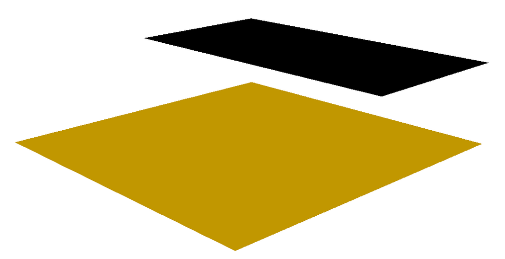
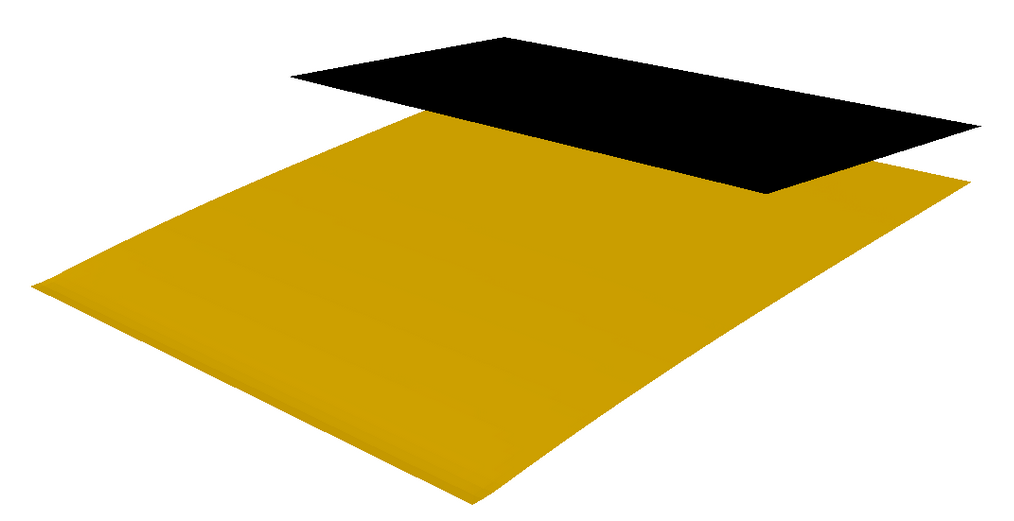
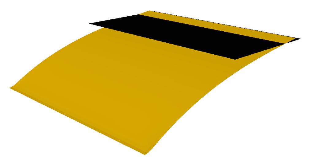
Figure 2. Top: Bilayer switching device consisting of a flexible single layer and a flexible bilayer strip that acts as a hinge. Middle: Switching device at times $t=0.0,0.9,$2.1\text{\,}\mathrm{s}$$. The bilayer region bends whereas the plate remains flat before hitting the obstacle (a)-(c). The device slightly penetrates the obstacle and then bends to accomodate the obstacle. Bottom: Experimental equilibrium states of the bilayer switching device without and with the obstacle.

To assess the intricate influence of the penalty parameter $\varepsilon$, we consider the same setting except for values of $\varepsilon=4\times 10^{-j}\,$\text{\,}\mathrm{m}\mathrm{m}^{4}{\rm MPa}^{-1}$$ for $j=4,...,9$. Cuts along the plane $\{x_{2}=0\}$ (perpendicular to the obstacle and the clamped side) of the plates stationary deformations are displayed in Figure 3. Plates are considered in a stationary state whenever

(21) $$\|\mathbf{y}_{h}^{k+1}-\mathbf{y}_{h}^{k}\|_{L_{2}(\omega)}+\|\nabla\nabla_{h}(\mathbf{y}_{h}^{k+1}-\mathbf{y}_{h}^{k})\|_{L_{2}(\omega)}\leq 10^{-5}.$$

On the one hand, the smallest value $\varepsilon$ corresponding to $j=9$ results in a plate which does not cross the obstacle but is influenced by the presence of the obstacle already when still far from the plate. On the other hand the largest value of $\varepsilon$ corresponding to $j=6$ results in a effective deformations without obstacle. Values of $\varepsilon$ for parameters $j=7,8$ yield a deformation crossing the planar obstacle by no more that the finite element meshsize.

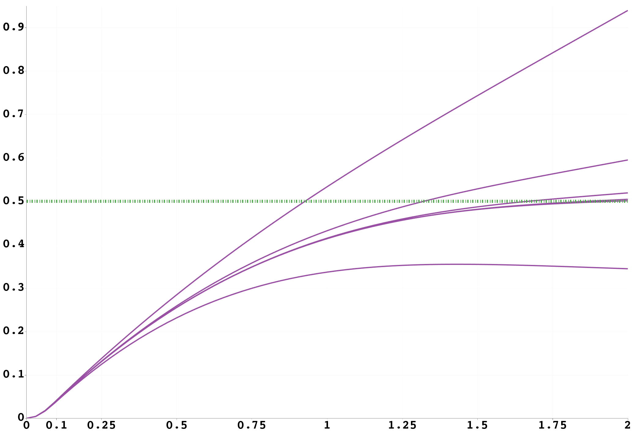
Figure 3. Cuts of stationary deformations along the plane $\{x_{2}=0\}$ of the bilayer switching device for (top to bottom curves) $\varepsilon=4\times 10^{-j}$\text{\,}\mathrm{m}\mathrm{m}^{4}{\rm MPa}^{-1}$$, $j=4,...,9$. Note that the curves corresponding to $j=8$ and $j=7$ are barely distinguishable and do not cross the obstacle $\{x_{3}=0.5\}$ more than the finite element meshsize $(=1/64)$. The horizontal line corresponds to the position of the obstacle.

It is worth mentioning that except the case $j=9$, all the stationary states (defined according to (21)) are reached at $T=$136.67\text{\,}\mathrm{s}$$ (44689 time iterations) while $j=9$ required $T=$182.739\text{\,}\mathrm{s}$$ (60913 time iterations). However, the dynamics for smaller $\varepsilon$ is influenced by the obstacle at early stages as illustrated in Figure 4. This is consistent with (19).

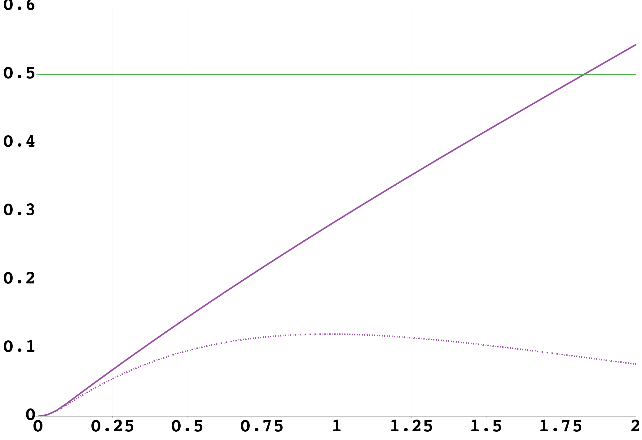
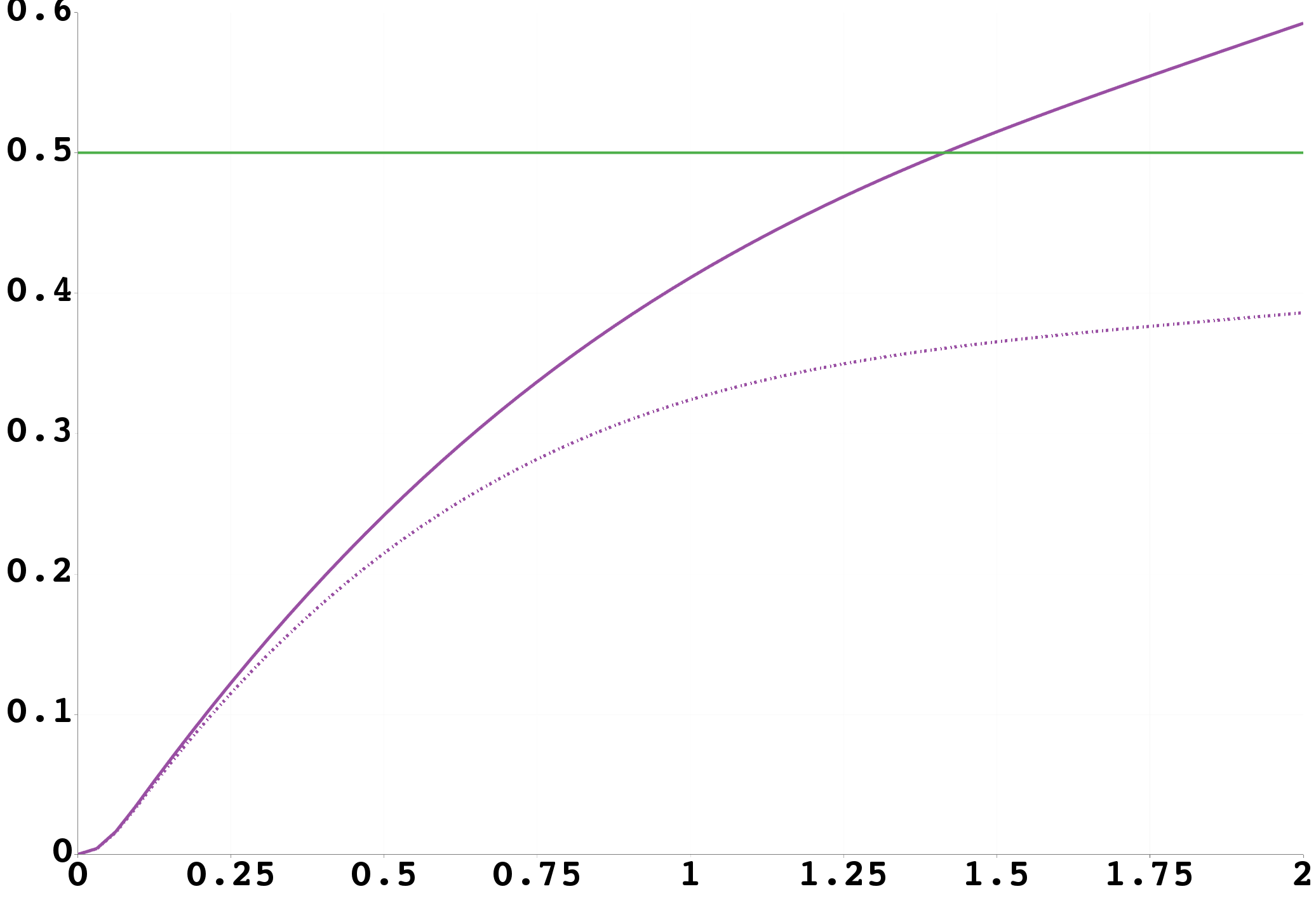
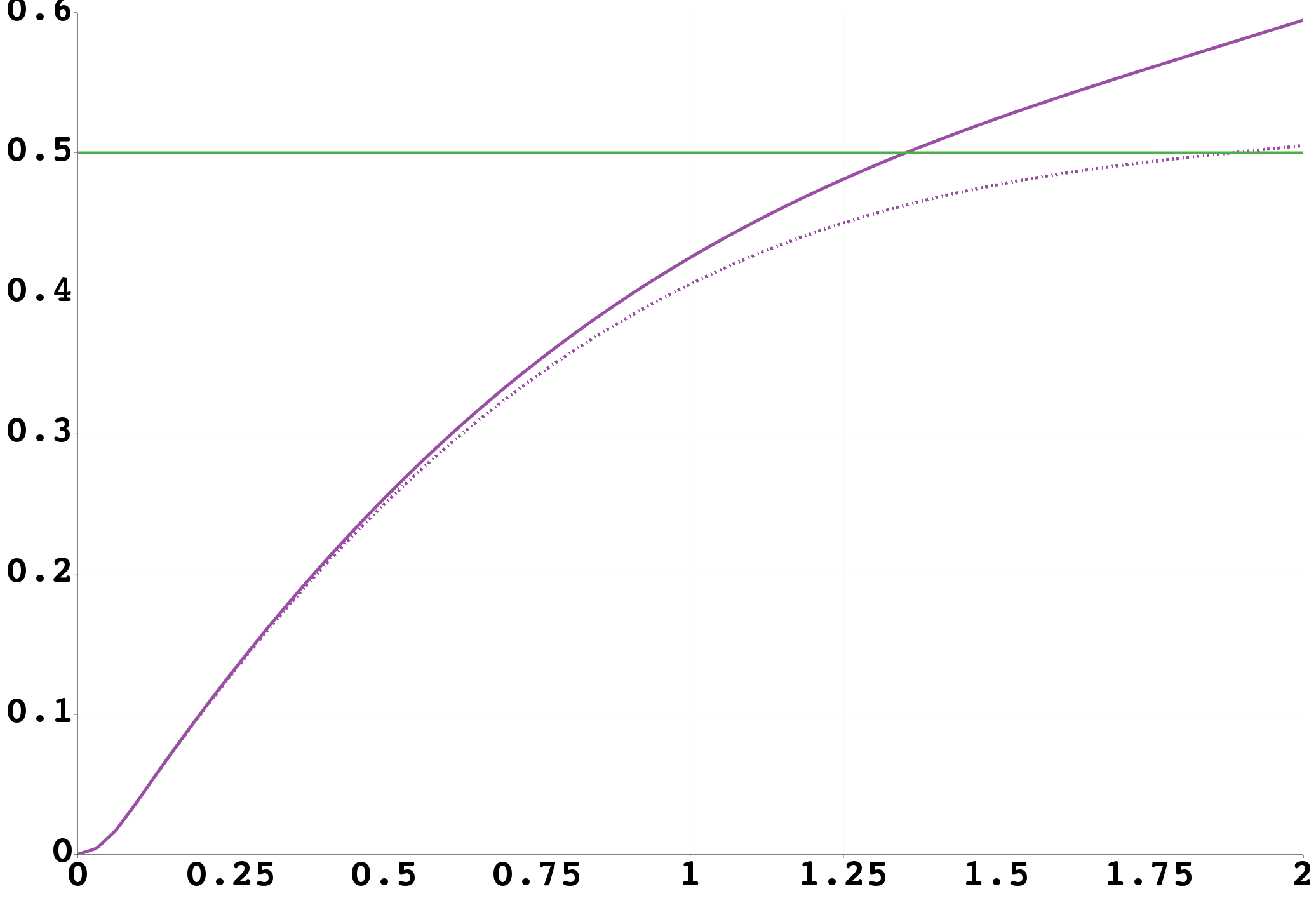
Figure 4. Cuts of deformations along the plane $\{x_{2}=0\}$ of the bilayer switching device for (top curve) $\varepsilon=$4\text{\times}{10}^{-5}\text{\,}\mathrm{m}\mathrm{m}^{4}{\rm MPa}^{-1}$$ and (bottom curve) $\varepsilon=$4\text{\times}{10}^{-7}\text{\,}\mathrm{m}\mathrm{m}^{4}{\rm MPa}^{-1}$$ and at times (left) $t=$2.4\text{\,}\mathrm{s}$$, (middle) $t=$4.8\text{\,}\mathrm{s}$$ and (right) $t=$7.2\text{\,}\mathrm{s}$$.

5.4. Dog-ear formation

To explore possible failure of controlled production of microtubes reported in [28, 33, 34] we consider a bilayer square $\omega=(-1,1)^{2}$ of side lengths $2.0\text{\,}\mathrm{mm}$ that is clamped and thermally insulated on the side $\partial_{D}\omega=\{-1\}\times[-1,1]$, namely $\mathbf{y}_{h}$ satisfies (20) and $\partial_{\mathbf{n}}\theta=0$ on $\partial_{D}\omega$. On the remaining part $\partial_{R}\omega=\partial\omega\setminus\partial_{D}\omega$ the plate is free and heated via external heat transfer obeying Newton’s law of cooling, i.e., the normal flux is proportional to temperature difference

$$\overline{\kappa}\nabla\theta\cdot\mathbf{n}=\overline{\eta}(\theta_{ext}-\theta)\qquad\text{on }\partial_{R}\omega$$

relative to the ambient temperature $\theta_{ext}=$50.0\text{\,}\mathrm{\SIUnitSymbolCelsius}$$. The experiment setup is sketched in Figure 5. For our numerical experiments we consider two different values of the effective thermal conductivity $\overline{\kappa}$ and heat capacity $\overline{\sigma}$ so that the resulting diffusivity differs by a factor 10, i.e., we consider

$$\text{(a)}\quad\overline{\kappa}/\overline{\sigma}=$0.1\text{\,}{\mathrm{mm}}^{2}\text{\,}{\mathrm{s}}^{-1}$,\qquad\text{(b)}\quad\overline{\kappa}/\overline{\sigma}=$1.0\text{\,}{\mathrm{mm}}^{2}\text{\,}{\mathrm{s}}^{-1}$.$$

We run Algorithm 3 (fully discrete scheme) for a uniform partitition of $\omega$ into subsquares with side lengths $h=2^{-6}\times$2.0\text{\,}\mathrm{mm}$$ and uniform time step $\tau=$5.0\text{\times}{10}^{-3}\text{\,}\mathrm{s}$$. Figure 5 displays snapshots of the approximate evolution for settings (a) and (b) for the respective times

$$t=0.0,\,1.0,\,2.5,\,16.0\times\overline{\kappa}/\overline{\sigma}.$$

Figure 5. Top: Bilayer plate clamped along one side $\partial_{D}\omega$ and heated via temperature difference with environment on $\partial_{R}\omega=\partial\omega\setminus\partial_{D}\omega$. Bottom: Bilayers heated via Robin condition on $\partial_{R}\omega$ with small (a) and large (b) diffusivity at different times. The gray scale represents the temperature within the plate (brightest = $0\text{\,}\mathrm{\SIUnitSymbolCelsius}$; darkest = $50\text{\,}\mathrm{\SIUnitSymbolCelsius}$). Small diffusivity leads to heat concentrations near $\partial_{R}\omega$ and strong localized bending behavior which resemble dog-ear formation.

We observe that the smaller diffusivity case (a) leads to accumulation of heat and higher temperatures in the vicinity the boundary $\partial_{R}\omega$ and in particular at the two corners belonging only to $\partial_{R}\omega$. This results in a stronger localized bending behavior for (a) and the formation of dog-ears which then prevent a controlled rolling up into a cylindrical shape. For larger diffusivity (b), heat distributes faster within the plate and the bending behavior is less localized.

5.5. Self-assembling box

We consider an arrangement of rigid plates and bilayer hinges that realizes a self-assembling and self-opening box actuated by temperature. We refer the reader to [29, 13] for related experiments. The relevant practical applications on this type of folding systems are on deployable structures such as drug delivery systems, deployable shelters with prefabricated walls. As in Subsection 5.3, the plate has $\overline{\alpha}=0$ and $\overline{\mu}$ that is $20$ larger than that of the hinge, so as to mimic a rigid plate insensitive to temperature. The geometry is sketched in Figure 6.

$t_{0}$	$t_{1}$	$t_{2}$
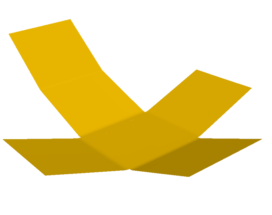
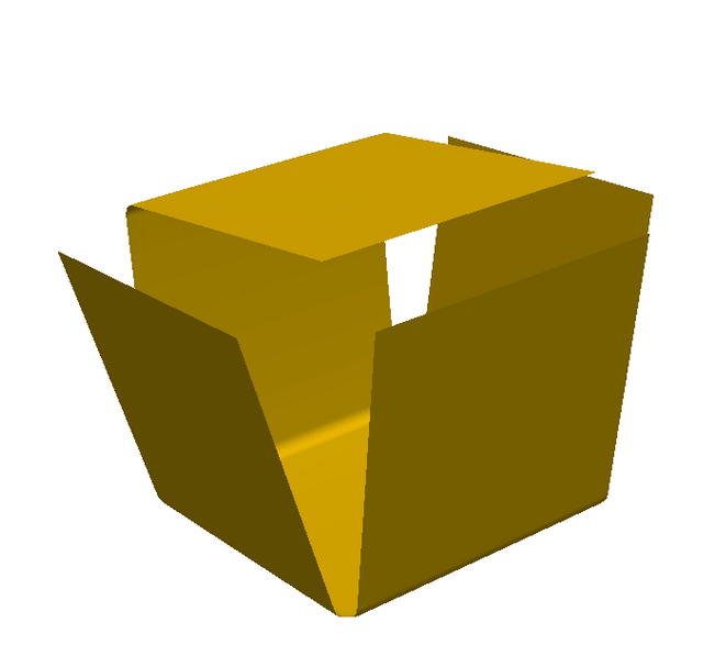
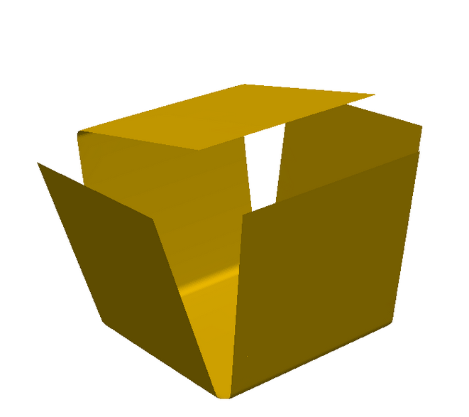
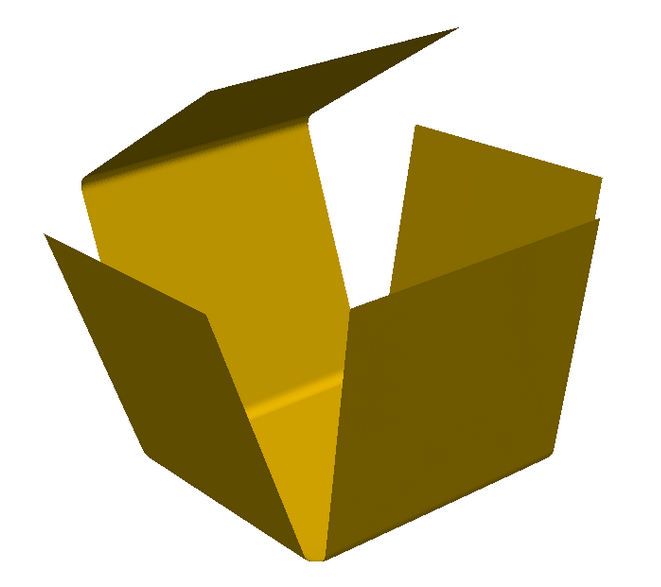
$t_{5}$	$t_{4}$	$t_{3}$

Figure 6. Top: Construction of a self-assembling box with 6 rigid plates connected by bilayer hinges. Bottom: Snapshots after $t=0.0,5.0,10.0,19.0,25.0,$30.0\text{\,}\mathrm{s}$$ of a self-assembling composite box at different times. The temperature distribution is nearly uniform throughout the evolution.

The square rigid plates have side lengths $1.0\text{\,}\mathrm{mm}$ and the hinges have widths $\pi\text{/}48\text{\,}\mathrm{mm}$. The central square, which is connected to four other squares, is assumed to be permanently attached to a substrate, and a constant heat source of $75.0\text{\,}\mathrm{\SIUnitSymbolCelsius}\text{\,}{\mathrm{s}}^{-1}$ is applied on a circle of radius $0.25\text{\,}\mathrm{mm}$ centered on this square during a period of $19.0\text{\,}\mathrm{s}$. Note that in that case, the heat equation reads

$$\partial_{t}\theta-10\Delta\theta=\left\{\begin{array}[]{ll}75.0&\qquad\text{in }\omega\times(0,19),\\ 0.0&\qquad\text{in }\omega\times(19,\infty).\end{array}\right.$$

When temperature increases the bilayer hinges start bending while the rigid plates remain undeformed, cf. Figure 6. For sufficient heating a box is formed which can be unfolded via external cooling. For our simulation we chose a uniform time step $\tau=$0.5\text{\,}\mathrm{s}$$ and a partition of $\omega$ into $3$ uniform quad refinements of each square plate, followed by $4$ quad refinements of elements in the hinges and additional local refinements to have at most one hanging node per side.

5.6. Deployable airfoil

We consider another arrangement of bilayer hinges and rigid plates shown in Figure 7 that models an initially flat device that can fold into an airfoil via external heating. Radical shape changes/folding of wing structures during flight can lead to high maneuverability of the plane and an efficient cruising that is adjustable to various flight envelopes. One example of morphing wing technology, i.e. z-shape folding, has been proposed by the Defense Advanced Research Projects Agency (DARPA), [17].

Figure 7. Top: Arrangement of bilayers and rigid plates for the construction of a deployable airfoil. Bottom: Snapshots of the folding process of the deployable airfoil at times $t=$ 0.0, 2.5, 500$\text{\,}\mathrm{s}$. The gray scale represents the temperature within the device (brightest = $0\text{\,}\mathrm{\SIUnitSymbolCelsius}$; darkest = $60\text{\,}\mathrm{\SIUnitSymbolCelsius}$).

The physical parameters are the same as in Subsection 5.5 except for $\overline{\kappa}/\overline{\sigma}=$0.1\text{\,}\mathrm{mm}\text{\,}{\mathrm{}}^{2}\text{\,}{\mathrm{s}}^{-1}$$ and the middle plate is fixed. As indicated in the sketch of Figure 7, the bilayer hinges bend into different directions, which is modeled by different signs of the effective expansion coefficients, i.e. $\overline{\alpha}=\pm 0.3$, or equivalently upon inverting the bilayer. The heat diffusion process is initiated by prescribing the temperature $\theta_{D}=$60.0\text{\,}\mathrm{\SIUnitSymbolCelsius}$$ at the Dirichlet boundary parts $\partial_{D}\omega$ where the hinges meet $\partial\omega$, and vanishing Neumann condition on the rest $\partial_{R}\omega=\partial\omega\setminus\partial_{D}\omega$ (i.e. $\overline{\eta}=0$). A simulation of the thermally driven folding process is illustrated in Figure 7.

5.7. Particle encapsulation

Thermally controlled bilayers for transporting particles at microscales have been tested experimentally in [27]. Once deployed in a desirable place, enclosed particles may be released via external cooling of the device. Similar mechanisms can be triggered by changing the pH concentration of a surrounding liquid. This may find exciting and important medical applications in targeted drug delivery.

To simulate the essential effects we consider a star-shaped configuration of a bilayer as shown in Figure 8. To start the encapsulation process we use a Robin boundary condition on the entire boundary with external temperature

$$\theta_{ext}=$100.0\text{\,}\mathrm{\SIUnitSymbolCelsius}$\qquad\text{on }\partial_{R}\omega=\partial\omega.$$

The boundary is mechanically free but we fix the deformation at the vertices of one element in the mesh $\mathcal{T}_{h}$ which contains the midpoint of the center square to guarantee well-posedness of our method, i.e., uniquely defined iterates in Algorithm 3 (fully practical scheme). If the device center has the coordinate $(0,0)$, then the obstacle consists of $5$ spheres $B_{i}$, $i=0,...,4$, each of radius $0.24\text{\,}\mathrm{m}\mathrm{m}$ and centered at $(0.28,0.28,0.25)$, $(0.72,0.28,0.25)$, $(0.28,0.72,0.25)$, $(0.72,0.72,0.25)$ and $(0.5,0.5,0.5)$ (all in $$\text{\,}\mathrm{m}\mathrm{m}$)$. At each vertex, the projection to the obstacle required by Algorithm 3 is approximated by the projection to the closest sphere. The obstacle models particles that are encapsulated by the deformed bilayer plate.

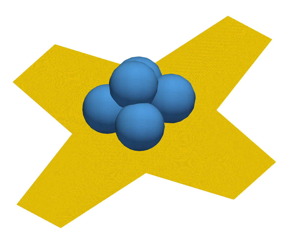
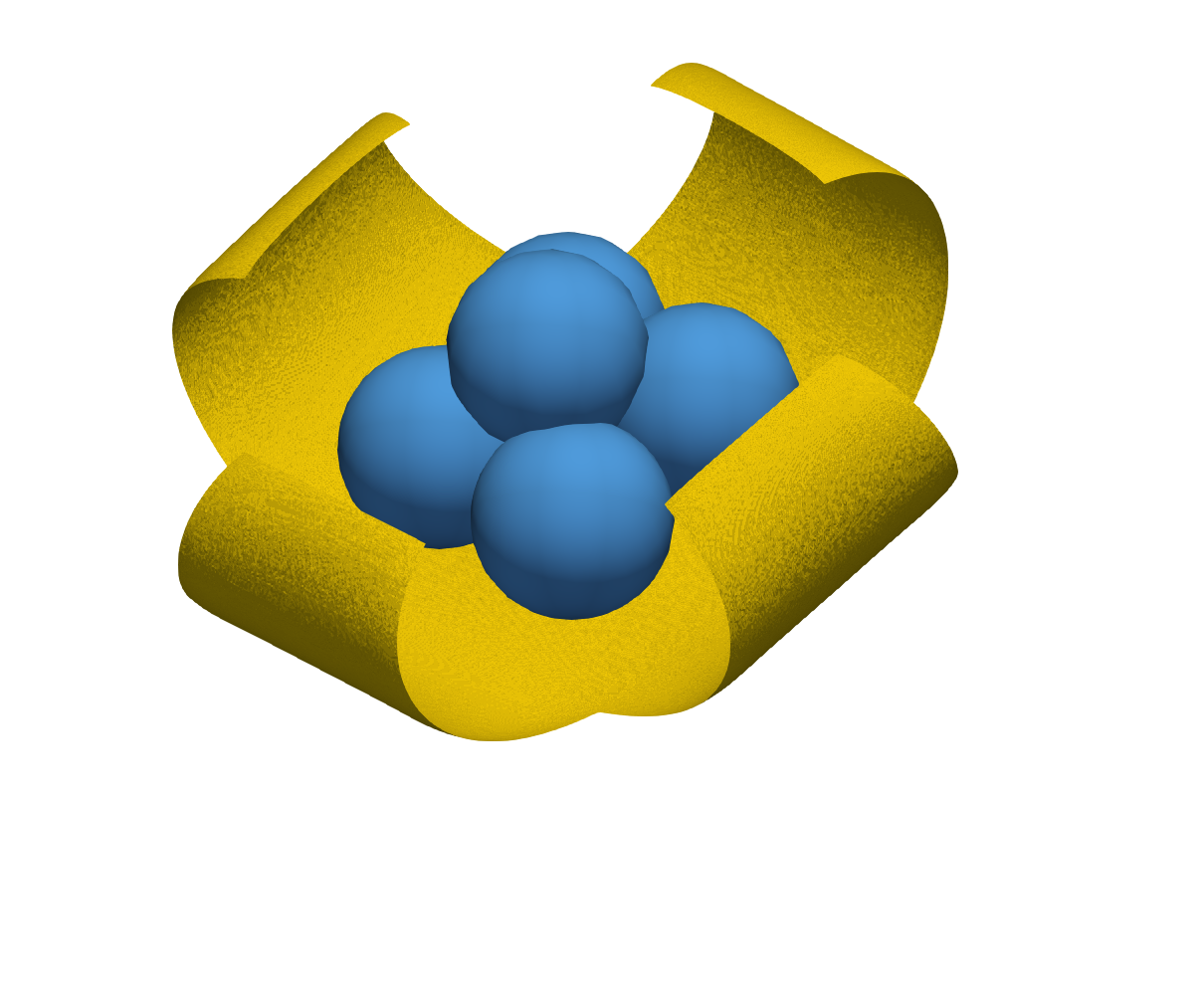
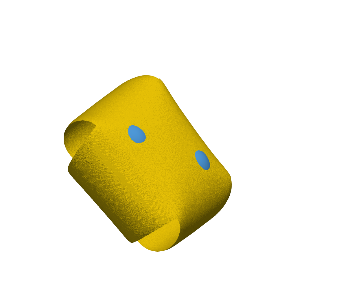
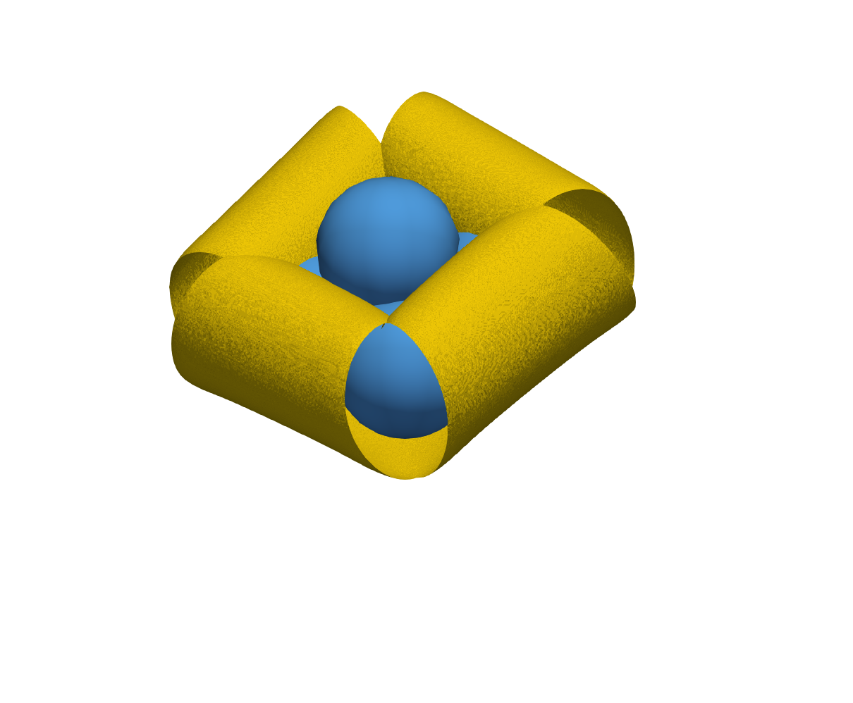
Figure 8. Top: Geometry of a bilayer plate that serves as a microcapsule and can be closed and opened via external heating and cooling. The dashed lines indicate the coarsest partition. Bottom: Folding of a micro-capsule enclosing 5 non-penetrable particles at times $t_{0}=$0.0\text{\,}\mathrm{s}$$, $t_{1}=$0.5\text{\,}\mathrm{s}$$ and $t_{2}=$1.0\text{\,}\mathrm{s}$$. The bottom left plot provides a different view at $t_{2}=$1.0\text{\,}\mathrm{s}$$ to illustrate the numerical penetration of the spherical obstacle by the plates, which is comparable to the finite element meshsize ($=1/64$). Note that the grey area depicted in the top figure can bend as well since only its corners are fixed. This effect can be reduced via higher resolution and smaller penalty parameter $\varepsilon$.

We construct the mesh $\mathcal{T}_{h}$ via 6 uniform quad refinements of the initial coarse partition of the domain $\omega$, indicated by the dashed lines in Figure 8. For our simulations we use the uniform time step $\tau=$2.5\text{\times}{10}^{-4}\text{\,}\mathrm{s}$$ and the penalization parameter $\varepsilon=$5.0\text{\times}{10}^{-8}\text{\,}\mathrm{m}\mathrm{m}^{4}{\rm MPa}^{-1}$$. Since $T=1s$ and $\mu_{0}=2\times 10^{3}{\rm MPa}$, this choice satisfies (19). Figure 8 depicts the encapsulation process of 5 non-penetrable and rigid spherical particles with radii $0.24\text{\,}\mathrm{mm}$. Penalization of the discrepancy between $y_{h}^{k+1}$ and $s_{h}^{k}$ in Algorithm 3 (fully practical scheme) does not prevent penetration of the obstacle, an effect that depends on the size of the penalization parameter $\varepsilon$ and the finite element meshsize and is discussed in Section 5.3. We refer to the lower part of Figure 8 that illustrates this feature. Reducing the size of $\varepsilon$ ameliorates this numerical artifact without making the algebraic system for $y_{h}^{k+1}$ of Algorithm 3 stiffer.

6. Conclusions

This paper develops a reduced model for the thermal actuation of bilayer plates consisting of a 4-th order nonlinear PDE and a 2-nd order diffusion in the mid-surface of a thin plate. The evolution is dictated by the latter whereas the former corresponds to a quasi-stationary reaction of the plate. We design a novel and effective finite element method for simulating large 3D deformations of slender planar structures, including the presence of obstacles. Several simulations illustrate the virtues of this approach.

The planar structures must be macroscopically compliant to allow for 3D shape changes with relatively small external stimuli. We study thin polymer materials composed of two layers which respond differently to thermal actuation, resulting in out of plane curvature changes and extremely large 3D deformations. The thin layer structures experience relatively small strain/stretch while undergoing large rotation. The interface between the two layers, or mid surface, is thus assumed to be perfectly bonded and inextensible, which leads to isometric deformations. The equations governing heat conduction and mechanical deformation decouple, i.e., the thermal effect induces plate deformations, but the latter do not affect heat conduction. This simplifies the solution process.

The algorithm takes advantage of several geometric properties valid for isometries, and advances in time with a semi-implicit scheme; the algebraic equations to be solved at each time step are linear. The only restrictions among discretization parameters come from achieving physically realistic dynamics in the presence of obstacles. Simulations of significant practical applications examine the feasibility of certain geometries and material parameters of polymers in attaining dramatic shape changes. This methodology could be used at the design stage, upon choosing material and geometric parameters as well as external stimuli and simulating shape reconfigurations prior to fabricating structures. This methodology is general and can be extented for more complex material models for active materials.

References

• [1] Alben, S., Balakrisnan, B., and Smela, E. Edge effects determine the direction of bilayer bending. Nano Letters 11, 6 (2011), 2280–2285. PMID: 21528897.
• [2] Ataka, M., Omodaka, A., Takeshima, N., and Fujita, H. Fabrication and operation of polyimide bimorph actuators for a ciliary motion system. Microelectromechanical Systems, Journal of 2, 4 (Dec 1993), 146–150.
• [3] Bartels, S. Approximation of large bending isometries with discrete Kirchhoff triangles. SIAM J. Numer. Anal. 51, 1 (2013), 516–525.
• [4] Bartels, S. Numerical methods for nonlinear partial differential equations., vol. 47 of Springer Series in Computational Mathematics. Springer, 2015.
• [5] Bartels, S., Bonito, A., and Nochetto, R. H. Bilayer plates: Model reduction, Γ-convergent finite element approximation, and discrete gradient flow. Comm. Pure Appl. Math. (2015), n/a–n/a.
• [6] Bassik, N., Abebe, B., Laflin, K., and Gracias, D. Photolithographically patterned smart hydrogel based bilayer actuators. Polymer 51 (2010), 6093–6098.
• [7] Batoz, J.-L., Bathe, K.-J., and Ho, L.-W. A study of three-node triangular plate bending elements. International Journal for Numerical Methods in Engineering 15, 12 (1980), 1771–1812.
• [8] Braess, D. Finite elements, third ed. Cambridge University Press, Cambridge, 2007. Theory, fast solvers, and applications in elasticity theory, Translated from the German by Larry L. Schumaker.
• [9] Dziuk, G., and Elliott, C. M. Finite elements on evolving surfaces. IMA J. Numer. Anal. 27, 2 (2007), 262–292.
• [10] Friesecke, G., James, R. D., and Müller, S. A theorem on geometric rigidity and the derivation of nonlinear plate theory from three-dimensional elasticity. Comm. Pure Appl. Math. 55, 11 (2002), 1461–1506.
• [11] Friesecke, G., James, R. D., and Müller, S. A hierarchy of plate models derived from nonlinear elasticity by gamma-convergence. Arch. Ration. Mech. Anal. 180, 2 (2006), 183–236.
• [12] Gordon, G. B., and Barth, P. W. Thermally-actuated microminiature valve, Oct. 22 1991. US Patent 5,058,856.
• [13] Janbaz, S., Hedayati, R., and Zadpoor, A. A. Programming the shape-shifting of flat soft matter: from self-rolling/self-twisting materials to self-folding origami. Mater. Horiz. (2016), –.
• [14] Kalaitzidou, K., and Crosby, A. Adaptive polymer particles. Applied Physics Letters 93, 041910 (2008).
• [15] Kuo, J.-N., Lee, G.-B., Pan, W.-F., and Lee, H.-L. Shape and thermal effects of metal films on stress-induced bending of micromachined bilayer cantilever. Japanese Journal of Applied Physics 44, 5R (2005), 3180.
• [16] Li, B., Chen, Q., Lee, D.-G., Woolman, J., and Carman, G. P. Development of large flow rate, robust, passive micro check valves for compact piezoelectrically actuated pumps. Sensors and Actuators A: Physical 117, 2 (2005), 325–330.
• [17] Love, M., Zink, P., Stroud, R., Bye, D., Rizk, S., and White, D. Demonstration of morphing technology through ground and wind tunnel tests. In 48th AIAA/ASME/ASCE/AHS/ASC Structures, Structural Dynamics, and Materials Conference (2007), p. 1729.
• [18] Magdanz, V., Guix, M., and Schmidt, O. Tubular micromotors: from microjets to spermbots. Robotics and Biomimetics 1, 1 (2014), 11.
• [19] Ogden, R. W. Nonlinear elastic deformations. Ellis Horwood Series: Mathematics and its Applications. Ellis Horwood Ltd., Chichester; Halsted Press [John Wiley & Sons, Inc.], New York, 1984.
• [20] Parthasarathy, S., Muliana, A., and Rajagopal, K. A fully coupled model for diffusion-induced deformation in polymers. Acta Mechanica 227 (2016), 837–856.
• [21] Schmidt, B. Minimal energy configurations of strained multi-layers. Calc. Var. Partial Differential Equations 30, 4 (2007), 477–497.
• [22] Schmidt, B. Plate theory for stressed heterogeneous multilayers of finite bending energy. J. Math. Pures Appl. (9) 88, 1 (2007), 107–122.
• [23] Schmidt, O., and Eberl, K. Thin solid films roll up into nanotubes. Nature 410 (2001), 168.
• [24] Smela, E., Inganös, O., and Lundström, I. Controlled folding of micrometer-size structures. Science 268, 5218 (1995), 1735–1738.
• [25] Smela, E., Inganös, O., Pei, Q., and Lundström, I. Electrochemical muscles: Micromachining fingers and corkscrews. Advanced Materials 5, 9 (1993), 630–632.
• [26] Srinivasa, A. On a class of gibbs potential-based nonlinear elastic models with small strain. Acta Mechanica 226 (2015), 571–583.
• [27] Stoychev, G., Puretskiy, N., and Ionov, L. Self-folding all-polymer thermoresponsive microcapsules. Soft Matter 7 (2011), 3277–3279.
• [28] Stoychev, G., Zakharchenko, S., Turcaud, S., Dunlop, J. W. C., and Ionov, L. Shape-programmed folding of stimuli-responsive polymer bilayers. ACS Nano 6, 5 (2012), 3925–3934. PMID: 22530752.
• [29] Suzuki, K., Shimoyama, I., and Miura, H. Insect-model based microrobot with elastic hinges. Microelectromechanical Systems, Journal of 3, 1 (Mar 1994), 4–9.
• [30] Tajeddini, V., and Muliana, A. Deformation of flexible and foldable electro-active composite structures. Composite Structures in press (2016).
• [31] Tzou, H., and Tseng, C. Distributed vibration control and identification of coupled elastic/piezoelectric systems: Finite element formulation and applications. Mechanical Systems and Signal Processing 5, 3 (1991), 215 – 231.
• [32] Wang, Q., and Wang, C. The constitutive relation and small scale parameter of nonlocal continuum mechanics for modelling carbon nanotubes. Nanotechnology 18, 7 (2007), 075702.
• [33] Ye, C., Nikolov, S. V., Calabrese, R., Dindarm, A., Alexeev, A., Kippelen, B., Kaplan, D. L., and Tsukruk, W. Self-(un)rolling biopolymer microstructures: Rings, tubules, and helical tubules from the same material. Angew. Chem. Int. Ed. 54 (2015).
• [34] Ye, C., Nikolov, S. V., Geryak, R. D., Calabrese, R., Ankner, J. F., Alexeev, A., Kaplan, D. L., and Tsukruk, V. V. Bimorph silk microsheets with programmable actuating behavior: Experimental analysis and computer simulations. ACS Applied Materials & Interfaces 8, 27 (2016), 17694–17706. PMID: 27308946.
• [35] Ye, C., and Tsukruk, V. V. Designing two-dimensional materials that spring rapidly into three-dimensional shapes. Science 347, 6218 (2015), 130–131.
• [36] Zhang, T., Li, X., and Gao, H. Defects controlled wrinkling and topological design in graphene. J. Mech. Phys. Solids (2014).