Exploring first-order phase transitions with population annealing

Abstract

Population annealing is a hybrid of sequential and Markov chain Monte Carlo methods geared towards the efficient parallel simulation of systems with complex free-energy landscapes. Systems with first-order phase transitions are among the problems in computational physics that are difficult to tackle with standard methods such as local-update simulations in the canonical ensemble, for example with the Metropolis algorithm. It is hence interesting to see whether such transitions can be more easily studied using population annealing. We report here our preliminary observations from population annealing runs for the two-dimensional Potts model with $q>4$, where it undergoes a first-order transition.

1 Introduction

Monte Carlo simulations are an indispensable tool for studies of a wide range of problems in statistical physics, including magnetic systems and other models on lattices as well as continuum models for polymers or colloids Landau and Binder (2015). While after 50 years of research the toolbox of simulational methods is quite well equipped with a rather diverse set of techniques, the vast majority belong to the kingdom of Markov chain approaches. Fundamentally different schemes such as sequential Monte Carlo Doucet et al. (2001) have received significantly less attention in this field (see, however, Ref. Grassberger (2002)). Population annealing (PA) Iba (2001); Hukushima and Iba (2003) is a technique combining elements of Markov chain and sequential Monte Carlo that has received relatively little attention to date Machta (2010); Machta and Ellis (2011); Wang et al. (2015a).

Since about 2005 the race towards higher and higher clock frequencies of CPUs and the resulting constant increase of the performance available from serial codes have come to end. High-performance computing has hence arrived in the era of massive parallelism, where additional computational power is essentially only available from a further multiplication of parallel computational cores Asanovic et al. (2006). This also led to a widespread application of hardware accelerators such as graphics processing units (GPUs) or Intel’s Xeon Phi devices, which currently feature several hundreds up to several thousands of cores per device. To be able to tap into this massively parallel computational power one needs parallel algorithms that scale well with the number of cores Owens et al. (2008). This is not one of the main strengths of Markov chain Monte Carlo (MCMC), which is inherently sequential, and parallelism can only be employed by sub-dividing the work in the updating step (domain decomposition) or by running multiple chains in parallel. The parallelism in the former approach is limited by the size of systems studied, while the latter has asymptotically vanishing efficiency as a larger and larger fraction of time needs to be spent on equilibration. This is where PA comes to the rescue. In PA one starts from a population of uncorrelated, random configurations at infinite temperature that are propagated down to low temperatures according to a well-defined stochastic protocol. For a population of size $R$ statistical errors decrease like $1/\sqrt{R}$ and bias as $1/R$ Machta and Ellis (2011); Wang et al. (2015a). The size of populations is mostly limited only by the available memory, but since memory is typically expected to scale with the number of cores this is not a real problem. The approach hence has theoretically excellent scaling properties, which are also borne out very well in practical implementations, for example on GPU Barash et al. .

An important application field for computer simulation studies in statistical physics are phase transitions and critical phenomena. While a lot of effort on the theoretical and computational side has been invested in the understanding of systems with continuous transitions, the vast majority of phase transitions in nature is of first order. They are characterized by the coexistence of two (or more) phases at the transition point as well as the phenomenon of metastability, i.e., the system remains in its present phase when crossing the transition point Binder (1987). These effects are accompanied by discontinuities in observable quantities such as the internal energy or magnetization across the transition, as well as dynamic effects such as hysteresis. In contrast to second-order transitions the correlation length remains finite. These features result in particular challenges for simulations of systems undergoing first-order transitions, including an exponential slowing down of the dynamics connecting the two phases due to a region of strongly suppressed states Janke (2003). Well known rather efficient simulation methods for this situation are the multicanonical approach Berg and Neuhaus (1992) and derived techniques such as Wang-Landau sampling Wang and Landau (2001). While population annealing has been used for simulations of spin-glass systems Wang et al. (2014, 2015a, 2015b) and the Ising model Weigel et al. , as well as for finding ground states of frustrated systems Wang et al. (2015c); Borovský et al. (2016), its behavior for systems undergoing first-order phase transitions has not been studied to date. We report here some preliminary results demonstrating the behavior of the PA algorithm for simulations in the first-order regime of the $q$-states Potts model in two dimensions Wu (1982).

The rest of the paper is organized as follows. In Sec. 2 we summarize the PA algorithm, while in Sec. 3 we introduce the Potts model and the relevant observables considered here. In Sec. 4 we report some properties of the distribution of energies and magnetizations in the population in the vicinity of a first-order transition. In Sec. 5 we show that PA is affected by hysteresis effects for discontinuous transitions. Section 6 is devoted to the illustration of a method of using the free-energy estimator provided by PA to determine the location of the transition point. Finally, Sec. 7 contains our conclusions.

2 The population annealing algorithm

Population annealing is a weighted sequential algorithm that performs a temperature sweep of a population of configurations (replicas) of the system under consideration Iba (2001); Hukushima and Iba (2003); Machta (2010). At each temperature step the population is resampled from the current distribution at inverse temperature $\beta=1/k_{B}T$ according to the probability distribution of energies at the target temperature $\beta+\Delta\beta$ that is estimated by reweighting. If the initial population is in equilibrium, which can be easily achieved by starting with random configurations produced by simple sampling at infinite temperature $\beta_{0}=0$, this procedure keeps the ensemble at equilibrium at all subsequent temperatures. In practice, however, the resampling leads to an exponential decline of diversity in the population, and in order to ensure fair sampling one needs to augment the procedure with further updates on the individual replicas that will typically be chosen according to a Markov chain scheme. In detail, the algorithm comprises the following steps:

1. Set up an equilibrium ensemble of $R=R_{0}$ independent copies (replicas) of the system at inverse temperature $\beta_{0}$. Often $\beta_{0}=0$, where this can be easily achieved.

2. To create an approximately equilibrated sample at $\beta_{i}>\beta_{i-1}$, resample configurations with their relative Boltzmann weight $\tau_{i}(E_{j})=\exp[-(\beta_{i}-\beta_{i-1})E_{j}]/Q_{i}$, where $Q_{i}=\sum_{j}\exp[-(\beta_{i}-\beta_{i-1})E_{j}]/R_{i-1}$.

3. Update each replica by $\theta$ rounds of an MCMC algorithm at inverse temperature $\beta_{i}$.

4. Calculate estimates for observable quantities ${\cal O}$ as population averages $\sum_{j}{\cal O}_{j}/R_{i}$.

5. Goto step 2 unless the target temperature $\beta_{K-1}$ has been reached.

While there is no theoretical restriction on the (inverse) temperature protocol $\beta_{0},\ldots$, $\beta_{K-1}$ to be used, we focus here on the simplest choice of constant steps, $\beta_{i}=\beta_{i-1}+\Delta\beta$. The resampling proportional to $\tau_{i}(E_{j})$ needs to take a normalization into account to ensure that the population size stays close to $R$. One possible implementation which is used here is to determine the number $r_{j}^{i}$ of copies of replica $j$ at temperature $\beta_{i}$ by drawing a random number from a Poisson distribution,

$$r_{j}^{i}\sim\mathrm{Pois}\left[(R/R_{i-1})\tau_{i}(E_{j})\right].$$ (1)

The new population size is then $R_{i}=\sum_{j}r^{i}_{j}$. The equilibration sweeps in step 3 can be chosen freely from any importance sampling algorithm. Here we use simple Metropolis single-spin flip updates.

A specialty of the PA approach is that it provides a natural estimate of the free energy through the expression Machta (2010)

$$-\beta_{i}F({\beta_{i}})=\ln Z_{\beta_{0}}+\sum_{m=1}^{i}\ln Q_{m},$$ (2)

that involves the reweighting factors $Q_{m}$. Here, $Z_{\beta_{0}}$ denotes the partition function at $\beta_{0}$ which needs to be known from other sources to get absolute free energies instead of just free-energy differences. This can be provided by explicit calculation for instance for $\beta_{0}=0$ or $\beta_{0}\to\infty$ or, more generally, through the application of high- and low-temperature expansions.

3 Potts model and observables

The Potts model is a natural generalization of the Ising model to spins with $q$ different states. The Hamiltonian in zero field is Wu (1982)

$${\cal H}=-J\sum_{\langle ij\rangle}\delta_{s_{i},s_{j}},$$ (3)

where the spins $s_{i}=1,2,...,q$ and $J>0$ is a ferromagnetic coupling constant. We study the model on the square lattice with nearest-neighbor interactions as indicated by the notation $\langle ij\rangle$ and set $J=1$ to fix units. Periodic boundary conditions are applied. For this specific setup, the transition temperature is exactly given by the relation $\beta_{t}=\ln{(1{+}\sqrt{q)}}$ that follows from the self-duality of the model Baxter (1973); Beffara and Duminil-Copin (2012). The model shows a first-order phase transition for $q>q_{c}$ and one finds that $q_{c}=4$ for the present setup Wu (1982). For $q\leq q_{c}$ the transition is continuous, with additional logarithmic corrections directly at $q_{c}$.

We use population annealing with a Metropolis update on single spins in step 3 of the algorithm described above to study the square-lattice Potts model for $q=6$, $8$, $10$, and $20$ (as well as, for comparison, $q=3$ in the second-order regime). The strength of the transition increases with $q$. The case $q=6$ is still relatively weakly first-order with a correlation length $\xi\approx 160$ at the transition point, while $q=20$ has a correlation length of $\xi\approx 3$ Borgs and Janke (1992). In contrast to regular MCMC, measurements in the PA approach are taken as ensemble averages over the population, and we thus record

$$\begin{split}\overline{E}(\beta_{i})&=\frac{1}{R_{i}}\sum_{j=1}^{R_{i}}E_{j},\\ \overline{M}(\beta_{i})&=\frac{1}{R_{i}}\sum_{j=1}^{R_{i}}M_{j}.\end{split}$$ (4)

Here, $E={\cal H}(\{s_{k}\})$ is the configurational energy, and the magnetization is defined on a finite lattice with $N=L^{2}$ spins via the number $\widetilde{M}$ of spins in the most common spin orientation,

$$\begin{split}M&=\frac{q\widetilde{M}-N}{q-1},\\ \widetilde{M}&=\max_{1\leq\alpha\leq q}\sum_{k=1}^{N}\delta_{s_{k},\alpha}.\end{split}$$ (5)

4 Behavior of the population

In a perfectly equilibrated PA simulation, the set of replicas at each temperature is a sample from the equilibrium energy distribution. For a system in the vicinity of a first-order transition one hence expects a rather wide distribution and, right at the transition point, a double peak indicating the phase coexistence there Janke (2003). In the left panel of Fig. 1 we show three representative histograms for a PA run with $R=10\,000$ and $\Delta\beta=0.01$ for the $q=6$ model with $L=32$. While one clearly sees a broadening of the energy distribution at the transition point, there is no double peak — and for these parameters we also do not find a double peak for any other temperature in the vicinity of the transition point. As we will see in more detail below in Sec. 5 this is a consequence of the metastability of the simulations.

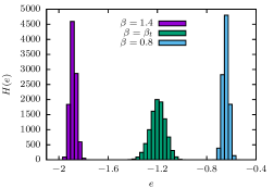
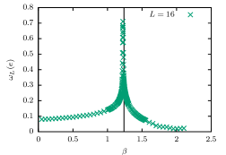
Figure 1: Left: Histograms of internal energies $e=E/N$ per spin of population members for a PA run for the $6$-state Potts model on a $32\times 32$ square lattice with periodic boundaries and parameters $R=10\,000$, $\theta=10$, $\Delta\beta=0.01$ at inverse temperatures $\beta=0.8$ in the high-temperature phase, $\beta=\beta_{t}\approx 1.24$ at the transition point, and $\beta=1.4$ in the ordered phase. Right: Full width at half maximum, $\omega_{L}(e)$, of the energy distribution over the population with $R=1000$ in a PA run for the $6$-state model and $L=16$, $\theta=100$. We used $\Delta\beta=1/N_{\beta}$ with $N_{\beta}=1000$ for $1.135\leq\beta\leq 1.305$ and $\Delta\beta=0.01$ otherwise, unless $\beta<0.995$ or $\beta>1.545$ in which case we used $\Delta\beta=0.05$.

We quantify the behavior of the histograms by systematically studying the widths $\omega_{L}(e)$ and $\omega_{L}(m)$ of the distributions of internal energies $e=E/N$ and magnetizations $m=M/N$ per spin, respectively, in the population. Here, the width is defined as the full width at half maximum of the corresponding histogram, i.e., if the maximum of the histogram is denoted as $H_{\mathrm{max}}$, it is the distance between the two intersections of the histogram with the horizontal line at $H_{\mathrm{max}}/2$. As is seen for an example run for $q=6$ and $L=16$ with $R=1000$ replicas and $\theta=100$ in the right panel of Fig. 1, the width of the energy histogram peaks close to the transition coupling. The same behavior is found for the magnetization histogram. We note that the widths are related to the specific heat and magnetic susceptibility, respectively, but these are more precisely a function of the variances of the distributions, so the relation is merely qualitative. Due to the metastability discussed above and the fact that we use a cooling (and not a heating) schedule, the quantities $\omega_{L}(e)$ and $\omega_{L}(m)$ correspond to the widths of the disordered peaks only Janke (2003).

In Tables 1 to 3 we collect our results for the widths $\omega_{L,\mathrm{max}}(e)$ and $\omega_{L,\mathrm{max}}(m)$ at the temperatures $T_{\mathrm{max}}(e)$ and $T_{\mathrm{max}}(m)$, respectively, where they are maximal. All data are averaged results from 200 independent runs. Table 1 shows the dependence on the number $q$ of Potts states — and hence the strength of the phase transition — as well as on the system size $L$. The size dependence of the positions of the maxima seems to be small, and it is possibly consistent with the shift of finite-size maxima proportional to $1/N$ expected for first-order transitions Janke (2003), but we did not perform a quantitative analysis. In Table 2 we summarize the observed dependence of histogram widths on the number $\theta$ of equilibration sweeps taken at each temperature. It is seen that the widths increase with $\theta$, indicating a gradual reduction of hysteresis with increasing $\theta$, thus ultimately revealing the double-peak nature of the energy and magnetization histograms at the transition point. Finally, in Table 3 we show the dependence of the maxima of the histogram widths on the temperature protocol for the case of using a spacing $\Delta\beta=1/N_{\beta}$ in inverse temperature in the vicinity of the transition for different values of $N_{\beta}$. It is seen that decreasing the size of temperature steps has an effect that is similar to that of increasing $\theta$ Weigel et al. .

Table 1: Maximal histogram widths and temperatures of maxima for the energy and magnetization for PA runs with $R=1000$ and $\theta=100$. We used $N_{\beta}=1000$ in all cases. To speed up the calculations, inverse temperature steps were chosen as follows. $q=6$: $\Delta\beta=1/N_{\beta}$ for $1.135\leq\beta\leq 1.305$ and $\Delta\beta=0.01$ otherwise, unless $\beta<0.995$ or $\beta>1.545$ where we used $\Delta\beta=0.05$. $q=8$: $\Delta\beta=1/N_{\beta}$ for $1.25\leq\beta\leq 1.42$ and $\Delta\beta=0.01$ otherwise, unless $\beta<1.11$ or $\beta>1.66$ where we used $\Delta\beta=0.05$. $q=10$: $\Delta\beta=1/N_{\beta}$ for $1.305\leq\beta\leq 1.475$ and $\Delta\beta=0.01$ otherwise, unless $\beta<1.165$ or $\beta>1.715$ where we used $\Delta\beta=0.05$. $q=20$: $\Delta\beta=1/N_{\beta}$ for $1.735\leq\beta\leq 1.905$ and $\Delta\beta=0.01$ otherwise, unless $\beta<1.595$ or $\beta>2.145$ where we used $\Delta\beta=0.05$.

	$L$	$\omega_{L,\mathrm{max}}(e)$	$T_{\mathrm{max}}(e)$	$\omega_{L,\mathrm{max}}(m)$	$T_{\mathrm{max}}(m)$
	16	$0.71$	$0.82$	$0.51$	$0.82$
	32	$0.39$	$0.81$	$0.41$	$0.81$
$q=6$	64	$0.23$	$0.80$	$0.40$	$0.80$
	128	$0.07$	$0.80$	$0.16$	$0.80$
	256	$0.03$	$0.80$	$0.055$	$0.79$
	16	$0.64$	$0.75$	$0.46$	$0.75$
	32	$0.34$	$0.74$	$0.36$	$0.74$
	64	$0.22$	$0.74$	$0.31$	$0.74$
$q=8$	96	$0.11$	$0.74$	$0.12$	$0.74$
	128	$0.074$	$0.74$	$0.09$	$0.73$
	192	$0.045$	$0.73$	$0.052$	$0.73$
	256	$0.032$	$0.73$	$0.037$	$0.73$
	16	$0.74$	$0.71$	$0.50$	$0.71$
	32	$0.38$	$0.70$	$0.43$	$0.70$
$q=10$	64	$0.20$	$0.69$	$0.27$	$0.69$
	128	$0.074$	$0.69$	$0.088$	$0.68$
	256	$0.032$	$0.69$	$0.026$	$0.68$
	16	$0.84$	$0.57$	$0.64$	$0.57$
	32	$0.57$	$0.57$	$0.48$	$0.57$
$q=20$	64	$0.18$	$0.57$	$0.17$	$0.56$
	128	$0.07$	$0.57$	$0.06$	$0.52$
	256	$0.029$	$0.57$	$0.018$	$0.52$

5 Hysteresis

One of the most characteristic features of first-order transitions is the occurrence of metastability, i.e., the system remains in one phase when the transition point is crossed even though the free energy of the other phase is lower there. The metastable states decay to the stable phases subject to perturbations on a time scale that depends on the cooling (or heating) rate. Only if one moves too far into the opposite phase regime, metastability disappears Binder (1987). To clearly reveal this effect in the present setup, we need to cross the phase boundary in both directions. This is possible through complementing the cooling run used in PA by an additional heating sweep. The algorithm described above in Sec. 2 is in fact independent of the sign of $\Delta\beta$, so a negative $\Delta\beta$ corresponding to a heating run is a perfectly valid choice.

To fulfill the preconditions of the approach, we only need to make sure that the starting population, which in contrast to the cooling run is now at the lowest temperature, is a well equilibrated sample. If we start runs deep in the ordered phase, however, this can easily be achieved by simulating the ensemble for a few sweeps of local updates at this lowest temperature. Alternatively, one might directly prepare the population in the ground-state manifold. For the present case, this corresponds to a uniform distribution of replicas over the $q$ ground states, i.e.,

$$s_{k}=\alpha,\;\;\;k=1,\ldots,N,$$ (6)

where $\alpha$ is an integer random variable with uniform distribution, ${\mathbb{P}}(\alpha=j)=1/q$. This corresponds to an equilibrium sample for $T=0$. In practice, it is an excellent approximation also for small $T>0$, and we start our runs at $\beta=3.0$.

The difference in energies between cooling and heating runs is shown for $q=3$, $q=6$ and $q=10$ and $L=32$ in the left panel of Fig. 2. The heating runs use the same temperature sequence as the cooling runs (but in reverse order). While in the second-order regime for $q=3$ the cooling and heating curves coincide within statistical errors, as expected, this is not the case for the first-order models with $q=6$ and $q=10$. This hysteresis effect increases with the strength of the transition and hence with the value of $q$. As the vertical dashed lines indicate, the area in the hysteresis loop is approximately, but clearly not perfectly divided in half by the asymptotic transition line Berg et al. (2004). We thus see clearly that PA in its standard setup is not able to equilibrate the population in the vicinity of the transition point. Still, the resampling strongly reduces the hysteresis effect, at least for the small system size considered here. This is illustrated in the right panel of Fig. 2, where we compare PA runs with and without resampling.

Table 2: Maximal histogram widths and temperatures of maxima for the energy and magnetization for the $8$-state Potts model on an $L=64$ lattice with $R=1000$ replicas as a function of $\theta$. The other parameters were chosen as explained in the caption of Table 1.

$\theta$	$\omega_{L,\mathrm{max}}(e)$	$T_{\mathrm{max}}(e)$	$\omega_{L,\mathrm{max}}(m)$	$T_{\mathrm{max}}(m)$
10	$0.10$	$0.73$	$0.14$	$0.72$
25	$0.13$	$0.74$	$0.20$	$0.73$
50	$0.17$	$0.74$	$0.23$	$0.74$
100	$0.22$	$0.74$	$0.31$	$0.74$
200	$0.28$	$0.74$	$0.39$	$0.74$
500	$0.29$	$0.74$	$0.36$	$0.74$
1000	$0.34$	$0.74$	$0.42$	$0.74$

Table 3: Maximal histogram widths and temperatures of maxima for the energy and magnetization for the $8$-state Potts model on an $L=64$ lattice with $R=1000$ replicas and $\theta=100$ sweeps as a function of the number $N_{\beta}$ of temperature steps in the vicinity of the transition coupling $\beta_{t}$. The temperature protocol is described in detail in the caption of Table 1.

$N_{\beta}$	$\omega_{L,\mathrm{max}}(e)$	$T_{\mathrm{max}}(e)$	$\omega_{L,\mathrm{max}}(m)$	$T_{\mathrm{max}}(m)$
100	$0.11$	$0.73$	$0.15$	$0.72$
200	$0.13$	$0.74$	$0.21$	$0.72$
500	$0.17$	$0.74$	$0.27$	$0.73$
1000	$0.23$	$0.74$	$0.34$	$0.74$
2000	$0.27$	$0.74$	$0.38$	$0.74$

To additionally illustrate the hysteresis effect in PA, we produced animations of the temperature sweeps showing the evolution of a randomly picked replica in the PA population for the two cases of increasing and decreasing temperatures. These videos are available in the supplementary material sup . Two videos show annealing (cooling) of the square lattice of $64\times 64$ spins for $q=6$ (correlation length $\xi\approx 160$) and for $q=20$ ($\xi\approx 3$). A further two videos show the heating runs for the same models. As is clearly visible, the ordering and disordering occurs in a way that is not symmetric between cooling and heating, indicative of the hysteresis and metastability. Note that the $q=6$ model with its large correlation length at the transition point shows similarities to the ordering behavior of a system with a continuous transition as for the given example $L=64\ll\xi\approx 160$.

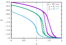
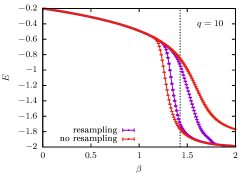
Figure 2: Left: Internal energy as measured in cooling runs (right curve of each color) and heating runs (left curve of each color) for $q=3$, $q=6$ and $q=10$ from PA runs for $L=32$ and $R=10\,000$ with $\theta=10$ and $\Delta\beta=0.01$. It is clearly visible that hysteresis occurs in the first-order cases $q=6$ and $q=10$, but not for the second-order model with $q=3$. The vertical dashed lines show the asymptotic transition points at $\beta_{t}=\ln(1+\sqrt{q})$. Right: The data for $q=10$ as shown on the left compared to the data for equivalent PA runs with the resampling step turned off.

6 The free energy

A classical method for the determination of the phase boundary in first-order transitions is the comparison of the free energies of the two phases as a function of the control parameter, here the temperature. The transition occurs where the two pure-phase branches of the free energy cross Janke (2003); Landau and Binder (2015). In standard Monte Carlo simulations it is not straightforward to produce reliable estimates of the free energy, as it cannot be directly derived from a configurational observable. The standard approach is through thermodynamic integration, which relies on the relation $E=\partial(\beta F)/\partial\beta$, such that a numerical integral of the internal energy over a temperature range will yield an estimate for the difference of free energies at the endpoints of the interval Landau and Binder (2015). The absolute normalization is additionally derived from exact calculations for $Z_{\beta_{0}}$ as indicated below Eq. (2) or from high- or low-temperature series expansions Janke (2003).

In PA, a reliable estimator of free energies is explicitly provided through the resampling factors that are combined in the estimator Eq. (2). For the case of the cooling schedule, we start at $\beta_{0}=0$ and hence we have $Z_{\beta_{0}}=q^{N}$. For the heating runs, on the other hand, we note that

$$Z_{\beta\to\infty}=\lim_{\beta\to\infty}\sum_{\{s_{k}\}}e^{-\beta{\cal H}(\{s_{k}\})}=\lim_{\beta\to\infty}q\,e^{-\beta E_{0}},$$ (7)

where $E_{0}$ is the ground-state energy that equals $E_{0}=-2N$ for the square-lattice model with periodic boundaries studied here. The free energy in this limit hence becomes

$$-\frac{\beta F_{\beta\to\infty}}{N}=\frac{\ln q}{N}-\beta e_{0},$$ (8)

where $e_{0}=E_{0}/N=-2$.

In Fig. 3 we show the resulting free-energy estimates from cooling runs starting from $\beta_{0}=0$ as compared to heating runs started from an equidistribution in the ground states of the system at the initial inverse temperature $\beta_{K-1}=3$ and using the normalizations resulting from $Z_{\beta_{0}}$ and $Z_{\beta\to\infty}$. As is seen in the left panel, the two estimates coincide everywhere for the second-order cases of the Ising model (corresponding to $q=2$, but with a different normalization) and the $q=3$ Potts model, but differences appear for the first-order systems $q=6$ and $q=10$. As the right panel reveals, the two metastable free energies cross very close to the asymptotic critical point. From the simulations with $\Delta\beta=0.01$ we can only determine the crossing points with a resolution of $\Delta\beta$, and the locations of the crossings are consistent with the asymptotic $\beta_{t}=\ln(1+\sqrt{q})$ already for $L=32$ studied here. One can easily imagine using a finer temperature grid in the relevant temperature regime to improve on these results.

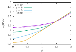
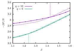
Figure 3: Left: Free energy of the Ising model and the $q=3$, $q=6$ and $q=10$ Potts models as estimated from PA runs with cooling (solid lines) and with heating (dashed lines). Parameters are $L=32$, $R=10\,000$, $\Delta\beta=0.01$ and $\theta=10$. For the Ising model and $q=3$, the two estimates coincide everywhere, whereas for the first-order cases $q=6$ and $q=10$ each estimate ceases to correspond to the equilibrium free energy as soon as the transition point is crossed. Right: Detail of the crossing of the metastable free energies for $q=6$ and $q=10$. Symbols with error bars are only shown for every fifth actual data point. The data for $q=10$ have been shifted vertically for clarity of presentation. The vertical dotted lines indicate the locations of the asymptotic transition points $\beta_{t}=\ln(1+\sqrt{q})$.

7 Conclusion

We have presented a preliminary report on the behavior of the population annealing algorithm when applied to a system with a first-order phase transition. As a well understood example system we considered the Potts model on the square lattice with $q>4$ states. While the resampling element reduces the effect of metastability and hysteresis, it is not able to remove it, at least without further modifications of the algorithm. Still, the possibility of reliably estimating free energies turns out to be a useful feature of the method also for the study of systems with first-order transitions as it appears to allow for a reasonably precise estimate of the transition point through the matching of the pure-phase free-energy branches. While population annealing in the present setup does not appear to be an ideal tool for systems with discontinuous transitions, the search for a variant of the approach using a modified ensemble and possibly modified update moves promises some improvement in this respect.