Disjointness graphs of segments in the space

Abstract

The disjointness graph $G=G({\cal S})$ of a set of segments ${\cal S}$ in ${{\mathbb{R}}}^{d}$, $d\geq 2,$ is a graph whose vertex set is ${\cal S}$ and two vertices are connected by an edge if and only if the corresponding segments are disjoint. We prove that the chromatic number of $G$ satisfies $\chi(G)\leq(\omega(G))^{4}+(\omega(G))^{3}$, where $\omega(G)$ denotes the clique number of $G$. It follows that $\cal S$ has $\Omega(n^{1/5})$ pairwise intersecting or pairwise disjoint elements. Stronger bounds are established for lines in space, instead of segments.

We show that computing $\omega(G)$ and $\chi(G)$ for disjointness graphs of lines in space are NP-hard tasks. However, we can design efficient algorithms to compute proper colorings of $G$ in which the number of colors satisfies the above upper bounds. One cannot expect similar results for sets of continuous arcs, instead of segments, even in the plane. We construct families of arcs whose disjointness graphs are triangle-free ($\omega(G)=2$), but whose chromatic numbers are arbitrarily large.

1 Introduction

Given a set of (geometric) objects, their intersection graph is a graph whose vertices correspond to the objects, two vertices being connected by an edge if and only if their intersection is nonempty. Intersection graphs of intervals on a line [H57], more generally, chordal graphs [B61, D61], and comparability graphs [D50], turned out to be perfect graphs, that is, for them and for each of their induced subgraph $H$, we have $\chi(H)=\omega(H)$, where $\chi(H)$ and $\omega(H)$ denote the chromatic number and the clique number of $H$, respectively. It was shown [HS58] that the complements of these graphs are also perfect. Based on the above results, Berge [B61] conjectured and Lovász [L72] proved that the complement of every perfect graph is perfect.

Most geometrically defined intersection graphs are not perfect. However, in many cases they still have nice coloring properties. For example, Asplund and Grünbaum [AG60] proved that every intersection graph $G$ of axis-parallel rectangles in the plane satisfies $\chi(G)=O((\omega(G))^{2})$. It is not known if the stronger bound $\chi(G)=O(\omega(G))$ also holds for these graphs. For intersection graphs of chords of a circle, Gyárfás [G85] established the bound $\chi(G)=O((\omega(G))^{2}4^{\omega(G)})$, which was improved to $O(2^{\omega(G)})$ in [KK97] and, recently, to $O(\omega\log\omega)$ by Chalermsook and Walczak [ChW19]. Here we have examples of graphs $G$ with $\chi(G)$ slightly superlinear in $\omega(G)$ [K88]. In some cases, there is no functional dependence between $\chi$ and $\omega$. The first such example was found by Burling [B65]: there are sets of axis-parallel boxes in ${{\mathbb{R}}}^{3}$, whose intersection graphs are triangle-free ($\omega=2$), but their chromatic numbers are arbitrarily large. Following Gyárfás and Lehel [GL83], we call a family $\cal G$ of graphs $\chi$-bounded if there exists a function $f$ such that all elements $G\in\cal G$ satisfy the inequality $\chi(G)\leq f(\omega(G))$. The function $f$ is called a bounding function for $\cal G$. Heuristically, if a family of graphs is $\chi$-bounded, then its members can be regarded “nearly perfect”. Consult [GL85, G87, K04] for surveys.

At first glance, one might believe that, in analogy to perfect graphs, a family of intersection graphs is $\chi$-bounded if and only if the family of their complements is. Burling’s above mentioned constructions show that this is not the case: the family of complements of intersection graphs of axis-parallel boxes in ${{\mathbb{R}}}^{d}$ is $\chi$-bounded with bounding function $f(x)=O(x\log^{d-1}x)$, see [K91]. More recently, Pawlik, Kozik, Krawczyk, Lasoń, Micek, Trotter, and Walczak [PKK14] have proved that Burling’s triangle-free graphs can be realized as intersection graphs of segments in the plane. Consequently, the family of these graphs is not $\chi$-bounded either. On the other hand, the family of their complements is, see Theorem 0.

To simplify the exposition, we call the complement of the intersection graph of a set of objects their disjointness graph. That is, in the disjointness graph two vertices are connected by an edge if and only if the corresponding objects are disjoint. Using this terminology, the following is a direct consequence of a result of Larman, Matoušek, Pach, and Törőcsik.

Theorem 0. [LMPT94] The family of disjointness graphs of segments in the plane is $\chi$-bounded. More precisely, every such graph $G$ satisfies the inequality $\chi(G)\leq(\omega(G))^{4}$.

For the proof of Theorem 0, one has to introduce four partial orders on the family of segments, and apply Dilworth’s theorem [D50] four times. Actually, the same argument also works systems of arbitrary $x$-monotone curves, instead of segments. (A continuous curve is called $x$-monotone if any line parallel to the $y$-axis intersects it in at most one point.) It was proved in [PaT19] that in this setting the order of magnitude or the upper bound $(\omega(G))^{4}$ cannot be improved.

One of the main results of this paper is a generalization of Theorem 0 to higher dimensions. We establish the following.

Theorem 1. The disjointness graph $G$ of any system of segments in ${{\mathbb{R}}}^{d},d\geq 2$ satisfies the inequality $\chi(G)\leq(\omega(G))^{4}+(\omega(G))^{3}$.

Moreover, there is a polynomial time algorithm that, given the segments corresponding to the vertices of $G$, finds a complete subgraph $K\subseteq G$ and a proper coloring of $G$ with at most $|V(K)|^{4}+|V(K)|^{3}$ colors.

Unfortunately, the technique applied in the plane does not seem to work in higher dimensions.

If we consider full lines in place of segments, we obtain stronger bounds.

Theorem 2. (i) Let $G$ be the disjointness graph of a set of lines in ${{\mathbb{R}}}^{d},\;d\geq 3.$ Then we have $\;\;\chi(G)\leq(\omega(G))^{3}.$

(ii) Let $G$ be the disjointness graph of a set of lines in the projective space ${{\mathbb{P}}}^{d},\;d\geq 3.$ Then we have $\;\;\chi(G)\leq(\omega(G))^{2}.$

In both cases, there are polynomial time algorithms that, given the lines corresponding to the vertices of $G$, find complete subgraphs $K\subseteq G$ and proper colorings of $G$ with at most $|V(K)|^{3}$ and $|V(K)|^{2}$ colors, respectively.

Note that the difference between the two scenarios comes from the fact that parallel lines in the Euclidean space are disjoint, but the corresponding lines in the projective space intersect.

Answering a question in an earlier draft of this paper, Norin [N17] showed that the family of intersection graphs of lines in ${{\mathbb{R}}}^{d}$ or ${{\mathbb{P}}}^{d}$, $d\geq 3$, is not $\chi$-bounded.

Most computational problems for geometric intersection and disjointness graphs are hard. It was shown by Kratochvíl and Nešetřil [KN90] and by Cabello, Cardinal, and Langerman [CCL13] that finding the clique number $\omega(G)$ resp. the independence number $\alpha(G)$ of disjointness graphs of segments in the plane are NP-hard. It is also known that computing the chromatic number $\chi(G)$ of disjointness and intersection graphs of segments in the plane is NP-hard [EET86]. Our next theorem shows that some of the analogous problems are also NP-hard for disjointness graphs of lines in space, while others are tractable in this case. In particular, according to Theorem 3(i), in a disjointness graph $G$ of lines, it is NP-hard to determine $\omega(G)$ and $\chi(G)$. In view of this, it is interesting that one can design polynomial time algorithms to find proper colorings and complete subgraphs in $G$, where the number of colors is bounded in terms of the size of the complete subgraphs, in the way specified in the closing statements of Theorems 1 and 2.

Theorem 3. (i) Computing the clique number $\omega(G)$ and the chromatic number $\chi(G)$ of disjointness graphs of lines in ${\mathbb{R}}^{3}$ or in ${\mathbb{P}}^{3}$ are NP-hard problems.

(ii) Computing the independence number $\alpha(G)$ of disjointness graphs of lines in ${\mathbb{R}}^{3}$ or in ${\mathbb{P}}^{3}$, and deciding for a fixed $k$ whether $\chi(G)\leq k$, can be done in polynomial time.

The bounding functions in Theorems 0, 1, and 2 are not likely to be optimal. As for Theorem 2 (i), we will prove that there are disjointness graphs $G$ of lines in $\mathbb{R}^{3}$ for which $\frac{\chi(G)}{\omega(G)}$ are arbitrarily large. Our best constructions for disjointness graphs $G^{\prime}$ of lines in the projective space satisfy $\chi(G^{\prime})\geq 2\omega(G^{\prime})-1$; see Theorem 2.3.

The proof of Theorem 1 is based on Theorem 0. Any strengthening of Theorem 0 leads to improvements of our results. For example, if $\chi(G)=O((\omega(G))^{\gamma})$ holds with any $3\leq\gamma\leq 4$ for the disjointness graph of every set of segments in the plane, then the proof of Theorem 1 implies the same bound for disjointness graphs of segments in higher dimensions. In fact, it is sufficient to verify this statement in $3$ dimensions. For $d\geq 4$, we can find a projection in a generic direction to the $3$-dimensional space that does not create additional intersections and then we can apply the $3$-dimensional bound. We focus on the case $d=3$.

It follows immediately from Theorem 0 that the disjointness (and, hence, the intersection) graph of any system of $n$ segments in the plane has a clique or an independent set of size at least $n^{1/5}$. Indeed, denoting by $\alpha(G)$ the maximum number of independent vertices in $G$, we have

$$\alpha(G)\geq\frac{n}{\chi(G)}\geq\frac{n}{(\omega(G))^{4}},$$

so that $\alpha(G)(\omega(G))^{4}\geq n$. Analogously, Theorem 1 implies that $\max(\alpha(G),\omega(G))\geq(1-o(1))n^{1/5}$ holds for disjointness (and intersection) graphs of segments in any dimension $d\geq 2$. For disjointness graphs of $n$ lines in $\mathbb{R}^{d}$ (respectively, in $\mathbb{P}^{d}$), we obtain that $\max(\alpha(G),\omega(G))$ is $\Omega(n^{1/4})$ (resp., $\Omega(n^{1/3})$). Using more advanced algebraic techniques, Cardinal, Payne, and Solomon [CPS16] proved the stronger bounds $\Omega(n^{1/3})$ (resp., $\Omega(n^{1/2})$).

If the order of magnitude of the bounding functions in Theorems 0 and 1 are improved, then the improvement carries over to the lower bound on $\max(\alpha(G),\omega(G))$. Despite many efforts [LMPT94, KPT97, K12] to construct intersection graphs of planar segments with small clique and independence numbers, the best known construction, due to Kynčl [K12], gives only

$$\max(\alpha(G),\omega(G))\leq n^{\log 8/\log 169}\approx n^{0.405},$$

where $n$ is the number of vertices. This bound is roughly the square of the best known lower bound.

Our next theorem shows that any improvement of the lower bound on $\max(\alpha(G),\omega(G))$ in the plane, even if it was not achieved by an improvement of the bounding function in Theorem 0, would also carry over to higher dimensions.

Theorem 4. If the disjointness graph of any set of $n$ segments in the plane has a clique or an independent set of size $\Omega(n^{\beta})$ for some fixed $\beta\leq 1/4$, then the same is true for disjointness graphs of segments in ${{\mathbb{R}}}^{d}$ for any $d>2$.

A continuous arc in the plane is called a string. One may wonder whether Theorem 0 can be extended to disjointness graphs of strings in place of segments. The answer is no, in a very strong sense.

Theorem 5. There exist triangle-free disjointness graphs of $n$ strings in the plane with arbitrarily large chromatic numbers. Moreover, we can assume that these strings are simple polygonal paths consisting of at most $4$ segments.

Recently, Mütze, Walczak, and Wiechert [MWW17] modified our constructions to obtain families of polygonal paths consisting of three segments each, which meet the requirements of Theorem 5 and any two paths cross at most once. It is not known whether one can find polygonal paths consisting of only two segments satisfying these conditions.

The following problems remain open.

Problem 6. (i) Is the family of disjointness graphs of polygonal paths, each consisting of at most two segments, $\chi$-bounded?

(ii) Is the previous statement true under the additional assumption that any two of the polygonal paths intersect in at most one point?

This paper is organized as follows. In the next section, we prove Theorem 2, which is needed for the proof of Theorem 1. Theorem 1 is established in Section 3. The proof of Theorem 4 is presented in Section 4. In Section 5, we construct several examples of disjointness graphs whose chromatic numbers are much larger than their clique numbers. In particular, we prove Theorem 5 and some similar statements. The last section contains the proof of Theorem 3 and remarks on the computational complexity of related problems.

2 Disjointness graphs of lines–Proof of Theorem 2

Claim 7. Let $G$ be the disjointness graph of a set of $n$ lines in ${\mathbb{P}}^{d}$. If $G$ has an isolated vertex, then $G$ is perfect.

Proof. Let $\ell_{0}\in V(G)$ be a line representing an isolated vertex of $G$. Consider the bipartite multigraph $H$ with vertex set $V(H)=A\cup B$, where $A$ consists of all points of $\ell_{0}$ that belong to at least one other line $\ell\in V(G)$, and $B$ is the set of all ($2$-dimensional) planes passing through $\ell_{0}$ that contain at least one other line $\ell\in V(G)$ different from $\ell_{0}$. We associate with any line $\ell\in V(G)$ different from $\ell_{0}$ an edge $e_{\ell}$ of $H$, connecting the point $p=\ell\cap\ell_{0}\in A$ to the plane $\pi\in B$ that contains $\ell$. Note that there may be several parallel edges in $H$. See Figure 1.

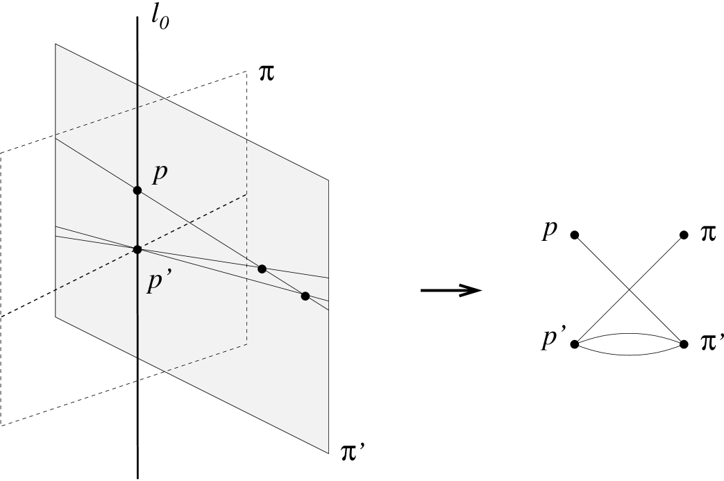
Figure 1: Construction of graph $H$ in the proof of Claim 7.

Observe that two lines $\ell,\ell^{\prime}\in V(G)\setminus\{\ell_{0}\}$ intersect if and only if $e_{\ell}$ and $e_{\ell^{\prime}}$ share an endpoint. This means that $G$ minus the isolated vertex $\ell_{0}$ is isomorphic to the complement of the line graph of $H$. The line graphs of bipartite multigraphs and their complements are known to be perfect. (For the complements of line graphs, this is the König-Hall theorem; see, e. g., [L93].) The graph $G$ can be obtained by adding the isolated vertex $\ell_{0}$ to a perfect graph, and is, therefore, also perfect. $\Box$

Proof of Theorem 2. We start with the proof of part (ii). Let $G$ be a disjointness graph of lines in ${\mathbb{P}}^{d}$. Let $C\subseteq G$ be a maximal clique in $G$. Clearly, $|C|\leq\omega(G)$. By the maximality of $C$, for every $\ell\in V(G)\setminus C$, there exists $c\in C$ that is not adjacent to $\ell$ in $G$. Hence, there is a partition of $V(G)$ into disjoint sets $V_{c},c\in C,$ such that $c\in V_{c}$ and $c$ is an isolated vertex in the induced subgraph $G[V_{c}]$ of $G$. Applying Claim 7 separately to each subgraph $G[V_{c}]$, we obtain

$$\chi(G)\leq\sum_{c\in C}\chi(G[V_{c}])=\sum_{c\in C}\omega(G[V_{c}])\leq|C|\omega(G)\leq(\omega(G))^{2}.$$

Now we turn to the proof of part (i) of Theorem 2. Let $G$ be a disjointness graph of lines in ${\mathbb{R}}^{d}$. Consider the lines in $V(G)$ as lines in the projective space ${\mathbb{P}}^{d}$, and consider the disjointness graph $G^{\prime}$ of these projective lines. Clearly, $G^{\prime}$ is a subgraph of $G$ with the lines $\ell$, $\ell^{\prime}\in V(G)$ adjacent in $G$ but not adjacent in $G^{\prime}$ if and only if $\ell$ and $\ell^{\prime}$ are parallel. Thus, an independent set in $G^{\prime}$ induces a disjoint union of complete subgraphs in $G$, where the vertices of each complete subgraph correspond to pairwise parallel lines. If $k$ is the maximal number of pairwise parallel lines in $V(G)$, then $k\leq\omega(G)$ and each independent set in $G^{\prime}$ can be partitioned into at most $k$ independent sets in $G$. Applying part (ii), we obtain

$$\chi(G)\leq k\chi(G^{\prime})\leq\omega(G)(\omega(G^{\prime}))^{2}\leq(\omega(G))^{3}.$$

Finally, we prove the last claim concerning polynomial time algorithms. In the proof of part (ii), we first took a maximal clique $C$ in $G$. Such a clique can be efficiently found by a greedy algorithm. The partition of $V(G)$ into subsets $V_{c},c\in C,$ such that $c\in V_{c}$ is an isolated vertex in the subgraph $G[V_{c}]$, can also be done efficiently. It remains to find a clique of maximum size and a proper coloring of each perfect graph $G[V_{c}]$ with the smallest number of colors. It is well known that for perfect graphs, both of these tasks can be completed in polynomial time. See e.g. Corollary 9.4.8 on page 298 of [GLS88]. Alternatively, notice that in the proof of Claim 7 we showed that $G[V_{c}]$ is, in fact, the complement of the line graph of a bipartite multigraph (plus an isolated vertex). Therefore, finding a maximum size complete subgraph corresponds to finding a maximum size matching in a bipartite graph, while finding an optimal proper coloring of $G[V_{c}]$ corresponds to finding a minimal size vertex cover in a bipartite graph. This can be accomplished by much simpler and faster algorithms than the general purpose algorithms developed for perfect graphs.

To finish the proof of the algorithmic claim for part (ii), we can simply output as $K$ the set $C$ or one of the largest maximum cliques in $G[V_{c}]$ over all $c\in C$, whichever is larger. We color each $V_{c}$ optimally, with pairwise disjoint sets of colors.

For the algorithmic claim about part (i), first color the corresponding arrangement of projective lines, and then refine the coloring by partitioning each color class into at most $k$ smaller classes, where $k$ is the maximum number of parallel lines in the arrangement. It is easy to find the value of $k$, just partition the lines into groups of parallel lines. Output as $K$ the set we found for the projective lines, or a set of $k$ parallel lines, whichever is larger. $\Box$

Theorem 8. (i) There exist disjointness graphs $G$ of families of lines in $\mathbb{R}^{3}$ for which the ratio $\chi(G)/\omega(G)$ is arbitrarily large.

(ii) For any $k$ one can find a system of lines in $\mathbb{P}^{3}$ whose disjointness graph $G$ satisfies $\omega(G)=k$ and $\chi(G)=2k-1$.

Proof. First, we prove (i). For some $m$ and $d$ to be determined later, consider the set $W_{m}^{d}$ of integer points in the $d$-dimensional hypercube $[1,m]^{d}$. That is, $W_{m}^{d}=\{1,2,\ldots,m\}^{d}$. A combinatorial line is a sequence of $m$ distinct points of $x^{1},\ldots,x^{m}\in W_{m}^{d}$ such that for every fixed $1\leq i\leq d$, the $i$th coordinates of $x^{j}$, $(x^{j})_{i}$, are either the same for all $1\leq j\leq m$ or we have $(x^{j})_{i}=j$ for all $1\leq j\leq m$. Note that the points of any combinatorial line lie on a geometric straight line. Let ${\cal L}$ denote the set of these geometric lines.

Let $G$ denote the disjointness graph of $\cal L$. Since each line in $\cal L$ passes through $m$ points of $W_{m}^{d}$, and $|W_{m}^{d}|=m^{d}$, we have $\omega(G)\leq m^{d-1}$. (It is easy to see that equality holds here, but we do not need this fact for the proof.)

Consider any proper coloring of $G$. The color classes are families of pairwise crossing lines in $\cal L$. Observe that any such family has a common point in $W_{m}^{d}$, except some families consisting of $3$ lines. Take an optimal proper coloring of $G$ with $\chi(G)$ colors, and split each $3$-element color class into two smaller classes. In the resulting coloring, there are at most $2\chi(G)$ color classes, each of which has a point of $W_{m}^{d}$ in common. This means that the set of at most $2\chi(G)$ points of $W_{m}^{d}$ (the “centers” of the color classes) “hits” every combinatorial line. By the density version of the Hales–Jewett theorem, due to Furstenberg and Katznelson [B98, FK91], if $d$ is large enough relative to $m$, then any set containing fewer than half of the points of $W_{m}^{d}$ will miss an entire combinatorial line. Choosing any $m$ and a sufficiently large $d$ depending on $m$, we conclude that $2\chi(G)\geq m^{d}/2$ and $\chi(G)/\omega(G)\geq m/4$.

Note that the family $\cal L$ consists of lines in ${\mathbb{R}}^{d}$. To find a similar family in 3-space, simply take the image of $\cal L$ under a projection to ${\mathbb{R}}^{3}$. One can pick a generic projection that does not change the disjointness graph $G$. This completes the proof of part (i). Note that the same construction does not work for projective lines, as the combinatorial lines in $W_{m}^{d}$ fall into $2^{d}-1$ parallel classes, so the chromatic number of the corresponding projective disjointness graph is smaller than $2^{d}$.

To establish part (ii), fix a positive integer $k$, and consider a set $S$ of $2k+1$ points in general position (no four in a plane) in $\mathbb{R}^{3}\subseteq\mathbb{P}^{3}$. Let $\cal L$ denote the set of $\binom{2k+1}{2}$ lines determined by them. Note that by the general position assumption, two lines in $\cal L$ intersect if and only if they have a point of $S$ in common. This means that the disjointness graph $G$ of $\cal L$ is isomorphic to the Kneser graph $G^{*}(2k+1,2)$ formed by all $2$-element subsets of a $(2k+1)$-element set. Obviously, $\omega(G^{*}(n,m))=\lfloor n/m\rfloor$, so $\omega(G)=k$. By a celebrated result of Lovász [L78], $\chi(G^{*}(n,m))=n-2m+2$ for all $n\geq 2m-1$. Thus, we have $\chi(G)=2k-1$, as claimed. $\Box$

3 Disjointness graphs of segments–Proof of Theorem 1

If all segments lie in the same plane, then by Theorem 0 we have $\chi(G)\leq(\omega(G))^{4}$. Our next theorem generalizes this result to the case where the segments lie in a bounded number of distinct planes.

Theorem 9. Let $G$ be the disjointness graph of a set of segments in $\mathbb{R}^{d},d>2,$ that lie in the union of $k$ two-dimensional planes. We have

$$\chi(G)\leq(k-1)\omega(G)+(\omega(G))^{4}.$$

Given the segments representing the vertices of $G$ and $k$ planes containing them, there is a polynomial time algorithm to find a complete subgraph $K\subseteq G$ and a proper coloring of $G$ with at most $(k-1)|V(K)|+|V(K)|^{4}$ colors.

Proof. Let $\pi_{1},\pi_{2},\ldots,\pi_{k}$ be the planes containing the segments. Partition the vertex set of $G$ into the classes $V_{1},V_{2},\ldots,V_{k}$ by putting a segment $s$ into the class $V_{i}$, where $i$ is the largest index for which $\pi_{i}$ contains $s$.

For $i=1,2,\ldots,k,$ we define subsets $W_{i},Z_{i}\subseteq V_{i}$ with $Z_{i}\subseteq W_{i}\subseteq V_{i}$ by a recursive procedure, as follows. Let $W_{1}=V_{1}$ and let $Z_{1}\subseteq W_{1}$ be a maximal size clique in $G[W_{1}]$.

Assume that the sets $W_{1},\dots,W_{i}$ and $Z_{1},\ldots,Z_{i}$ have already been defined for some $i<k$. Let $W_{i+1}$ denote the set of all vertices in $V_{i+1}$ that are adjacent to every vertex in $Z_{1}\cup Z_{2}\cup\ldots\cup Z_{i}$, and let $Z_{i+1}$ be a maximal size clique in $G[W_{i+1}]$. By definition, $\bigcup_{i=1}^{k}Z_{i}$ induces a complete subgraph in $G$, and we have

$$\sum_{i=1}^{k}|Z_{i}|\leq\omega(G).$$

Let $s$ be a segment belonging to $Z_{i}$, for some $1\leq i<k$. A point $p$ of $s$ is called a piercing point if $p\in\pi_{j}$ for some $j>i$. Notice that in this case, $s$ “pierces” the plane $\pi_{j}$ in a single point, otherwise we would have $s\subset\pi_{j}$, contradicting our assumption that $s\in V_{i}$. Letting $P$ denote the set of piercing points of all segments in $\bigcup_{i=1}^{k}Z_{i}$, we have

$$|P|\leq\sum_{i=1}^{k}(k-i)|Z_{i}|\leq(k-1)\sum_{i=1}^{k}|Z_{i}|\leq(k-1)\omega(G).$$

Let $V_{0}=V(G)\setminus\bigcup_{i=1}^{k}W_{i}$. We claim that every segment in $V_{0}$ contains at least one piercing point. Indeed, if $s\in V_{i}\setminus W_{i}$ for some $i\leq k$, then $s$ is not adjacent in $G$ to at least one segment $t\in Z_{1}\cup\ldots\cup Z_{i-1}$. Thus, $s$ and $t$ are not disjoint, and their intersection point is a piercing point, at which $t$ pierces the plane $\pi_{i}$.

Assign a color to each piercing point $p\in P$. Coloring every segment in $V_{0}$ by the color of one of its piercing points, we get a proper coloring of $G[V_{0}]$ with $|P|$ colors, so that $\chi(G[V_{0}])\leq|P|.$

For every $i\leq k$, all segments of $W_{i}$ lie in the plane $\pi_{i}$. Therefore, we can apply Theorem 0 to their disjointness graph $G[W_{i}]$, to conclude that $\chi(G[W_{i}])\leq(\omega(G[W_{i}]))^{4}$. By definition, $Z_{i}$ induces a maximum complete subgraph in $G[W_{i}]$, hence $|Z_{i}|=\omega(G[W_{i}])$ and $\chi(G[W_{i}])\leq|Z_{i}|^{4}$.

Putting together the above estimates, and taking into account that $\bigcup_{i=1}^{k}Z_{i}$ induces a complete subgraph in $G$, we obtain

$$\chi(G)\leq\chi(G[V_{0}])+\sum_{i=1}^{k}\chi(G[W_{i}])\leq|P|+\sum_{i=1}^{k}|Z_{i}|^{4}$$

$$\leq(k-1)\omega(G)+(\sum_{i=1}^{k}|Z_{i}|)^{4}\leq(k-1)\omega(G)+(\omega(G))^{4},$$

as required.

We can turn this estimate into a polynomial time algorithm as required, using the fact that the proof of Theorem 0 is constructive. In particular, we use that, given a family of segments in the plane, one can efficiently find a subfamily $K$ of pairwise disjoint segments and a proper coloring of the disjointness graph with at most $|K|^{4}$ colors. This readily follows from the proof of Theorem 0, based on the four easily computable (semi-algebraic) partial orders on the family of segments, introduced in [LMPT94].

Our algorithm finds the sets $V_{i}$, as in the proof. However, finding $W_{i}$ and a maximum size clique $Z_{i}\subseteq W_{i}$ is a challenge. Instead, we use the constructive version of Theorem 0 to find a $Z_{i}\subseteq W_{i}$ which is a clique but not necessarily the largest and a proper coloring of $G[W_{i}]$. The definition of $W_{i}$ remains unchanged. Next, the algorithm identifies the piercing points.

The algorithm outputs the clique $K=\bigcup Z_{i}$ and the coloring of $G$. The latter one is obtained by combining the previously constructed colorings of the subgraphs $G[W_{i}]$ (using disjoint sets of colors for different subgraphs), and coloring each remaining vertex by a previously unused color, associated with one of the piercing points the corresponding segment passes through. $\Box$

Proof of Theorem 1. Consider the set of all lines in the projective space $\mathbb{P}^{d}$ that contain at least one segment belonging to $V(G)$. Let $\bar{G}$ denote the disjointness graph of these lines. Obviously, we have $\omega(\bar{G})\leq\omega(G)$. Thus, Theorem 2(ii) implies that

$$\chi(\bar{G})\leq(\omega(\bar{G}))^{2}\leq(\omega(G))^{2}.$$

Let $C$ be the set of lines corresponding to the vertices of a maximum complete subgraph in $\bar{G}$. Fix an optimal proper coloring of $\bar{G}$. Suppose that we used $k$ “planar” colors (each such color is given to a set of lines that lie in the same plane) and $\chi(\bar{G^{\prime}})-k$ “pointed” colors (each given to the vertices corresponding to a set of lines passing through a common point).

Consider now $G$, the disjointness graph of the segments. Let $G_{0}$ denote the subgraph of $G$ induced by the set of segments whose supporting lines received one of the $k$ planar colors in the above coloring of $\bar{G}$. These segments lie in at most $k$ planes. Therefore, applying Theorem 9 to $G_{0}$, we obtain

$$\chi(G_{0})\leq(k-1)\omega(G_{0})+(\omega(G_{0}))^{4}\leq(k-1)\omega(G)+(\omega(G))^{4}.$$

For $i,1\leq i\leq\chi(\bar{G})-k,$ let $G_{i}$ denote the subgraph of $G$ induced by the set of segments whose supporting lines are colored by the $i$th pointed color. Its complement, $\overline{G_{i}}$, can be represented as the intersection graph of subtrees of a tree. Therefore, by the result of Gavril [G74], $\overline{G_{i}}$ is a chordal graph, that is, it contains no induced cycle of length larger than $3$. According to a theorem of Hajnal and Surányi [HS58], any graph with this property is perfect, consequently $G_{i}$ is also perfect. Therefore,

$$\chi(G_{i})=\omega(G_{i})\leq\omega(G).$$

Putting these bounds together, we obtain that

$$\chi(G)\leq\chi(G_{0})+\sum_{i=1}^{\chi(\bar{G})-k}\chi(G_{i})\leq(k-1)\omega(G)+(\omega(G))^{4}+\sum_{i=1}^{\chi(\bar{G})-k}\omega(G)$$

$$\leq((\omega(\bar{G}))^{2}-1)\omega(G)+(\omega(G))^{4}<(\omega(G))^{3}+(\omega(G))^{4}.$$

To prove the algorithmic claim in Theorem 1, we first apply the algorithm of Theorem 2 to the disjointness graph $\bar{G}^{\prime}$. We distinguish between planar and pointed color classes and find the subgraphs $G_{i}$. We output a coloring of $G$, where for each $G_{i},i>0$ we use the smallest possible number of colors ($G_{i}$ is perfect, so its optimal coloring can be found in polynomial time), and we color $G_{0}$ by the algorithm described in Theorem 9. The subgraphs $G_{i}$ are colored using pairwise disjoint sets of colors. We output the largest clique $K$ that we can find. This may belong to a subgraph $G_{i}$ with $i>0$, or may be found in $G_{0}$ or in $\bar{G}^{\prime}$ by the algorithms given by Theorem 9 or Theorem 2, respectively. (In the last case, we need to turn a clique in $\bar{G}^{\prime}$ into a clique of the same size in $G$, by picking an arbitrary segment from each of the pairwise disjoint lines.) $\Box$

4 Ramsey-type bounds in $\mathbb{R}^{2}$ vs. $\mathbb{R}^{3}$–Proof of Theorem 4

As we have pointed out in the Introduction, it is sufficient to establish Theorem 4 in $\mathbb{R}^{3}$. We rephrase Theorem 4 for this case in the following form.

Theorem 10. Let $f(m)$ be a function with the property that for any disjointness graph $G$ of a system of segments in $\mathbb{R}^{2}$ with $\max(\alpha(G),\omega(G))\leq m$ we have $|V(G)|\leq f(m).$

Then for any disjointness graph $G$ of a system of segments in $\mathbb{R}^{3}$ with $\max(\alpha(G),\omega(G))$ $\leq m$ we have $|V(G)|\leq f(m)+m^{4}.$

Applying Theorem 10 with $f(k)=ck^{1/\beta}$, Theorem 4 immediately follows. We prove Theorem 10 by adapting the proof of Theorem 9.

Proof of Theorem 10. Let $G$ be the disjointness graph of a set of segments in $\mathbb{R}^{3}$ with $\omega(G)\leq m$ and $\alpha(G)\leq m$.

First, assume that all segments lie in the union of $k$ planes, for some $k\geq 1$. Define the sets of vertices $V_{i}$, $W_{i}$, and $Z_{i}$ for every $1\leq i\leq k$, as in the proof of Theorem 9, and let $V_{0}=V(G)\setminus\bigcup_{i=1}^{k}W_{i}$. Since all elements of $W_{i}$ lie in the same plane, the subgraph induced by them is a planar segment disjointness graph for every $i\geq 1$. We can clearly represent these graphs by segments in a common plane $\pi$ such that two segments intersect if and only they come from the same set $W_{i}$ and there they intersect. In this way, we obtain a system of segments in the plane whose disjointness graph $G^{*}$ is the join of the graphs $G[W_{i}]$, i.e., $G^{*}$ is obtained by taking the disjoint union of $G[W_{i}]$ (for all $i\geq 1$) and adding all edges between $W_{i}$ and $W_{j}$ for every pair $i\neq j$. Clearly, we have

$$\omega(G^{*})=\sum_{i=1}^{k}\omega(G[W_{i}])=\sum_{i=1}^{k}|Z_{i}|\leq\omega(G)\leq m,$$

and

$$\alpha(G^{*})=\max_{i=1}^{k}\alpha(G[W_{i}])\leq\alpha(G)\leq m.$$

By our assumption, $G^{*}$ has at most $f(m)$ vertices, so that $\sum_{i=1}^{k}|W_{i}|\leq f(m).$ As we have seen in the proof of Theorem 9, the total number of piercing points is at most $(k-1)\sum_{i=1}^{k}|Z_{i}|\leq(k-1)\omega(G)<km$, and each segment in $V_{0}$ contains at least one of them. Each piercing point is contained in at most $m$ segments, because these segments induce an independent set in $G$. Thus, we have $|V_{0}|<km^{2}$ and

$$|V(G)|=|V_{0}|+\bigcup_{i=1}^{k}|W_{i}|<km^{2}+|V(G^{*})|\leq km^{2}+f(m).$$

Now we turn to the general case, where there is no bound on the number of planes containing the segments. As in the proof of Theorem 1, we consider the disjointness graph $\bar{G}$ of the supporting lines of the segments in the projective space $\mathbb{P}^{3}$. Clearly, we have $\omega(\bar{G})\leq\omega(G)\leq m$, so by Theorem 1 we have $\chi(\bar{G})\leq m^{2}$. Following the proof of Theorem 1, take an optimal coloring of $\bar{G}$, and let $G_{0}$ denote the subgraph of $G$ induced by the segments whose supporting lines received one of the planar colors. Letting $k$ denote the number of planar colors, for every $i,1\leq i\leq\omega(\bar{G})-k,$ let $G_{i}$ denote the subgraph of $G$ induced by the set of segments whose supporting lines received the $i$th pointed color. As in the proof of Theorem 1, every $G_{i},i\geq 1$ is perfect and, hence, its number of vertices satisfies

$$|V(G_{i})|\leq\chi(G_{i})\alpha(G_{i})\leq\omega(G_{i})\alpha(G_{i})\leq\omega(G)\alpha(G)\leq m^{2}.$$

The segments belonging to $V(G_{0})$ lie in at most $k$ planes. In view of the previous paragraph, $|V(G_{0})|\leq km^{2}+f(m)$ vertices. Combining the above bounds, we obtain

$$|V(G)|=|V(G_{0})|+\sum_{i=1}^{\chi(\bar{G})-k}|V(G_{i})|\leq km^{2}+f(m)+(\chi(\bar{G})-k)m^{2}$$

$$\leq km^{2}+f(m)+(m^{2}-k)m^{2}\leq f(m)+m^{4},$$

which completes the proof. $\Box$

5 Constructions–Proof of Theorem 5

The aim of this section is to describe various arrangements of geometric objects in 2, 3, and 4 dimensions with triangle-free disjointness graphs, whose chromatic numbers grow logarithmically with the number of objects. (This is much faster than the rate of growth in Theorem 8.) Our constructions can be regarded as geometric realizations of a sequence of graphs discovered by Erdős and Hajnal.

Definition 11. [EH64]. Given $m>1$, let $H\noindent_{m}$, the $m$th shift graph, be a graph whose vertex set consists of all ordered pairs $(i,j)$ with $1\leq i<j\leq m$, and two pairs $(i,j)$ and $(k,l)$ are connected by an edge if and only if $j=k$ or $l=i$.

Obviously, $H_{m}$ is triangle-free for every $m>1$. It is not hard to show (see, e.g., [L93], Problem 9.26) that $\chi(H_{m})=\lceil\log_{2}m\rceil$. Therefore, Theorem 5 follows directly from part (vii) of the next theorem.

Theorem 12. For every $m$, the shift graph $H_{m}$ can be obtained as a disjointness graph, where each vertex is represented by

(i) a line minus a point in ${\mathbb{R}}^{2}$;

(ii) a two-dimensional plane in ${\mathbb{R}}^{4}$;

(iii) the intersection of two general position half-spaces in ${\mathbb{R}}^{3}$;

(iv) the union of two segments in ${\mathbb{R}}^{2}$;

(v) a triangle in ${\mathbb{R}}^{4}$;

(vi) a simplex in ${\mathbb{R}}^{3}$;

(vii) a polygonal curve in ${\mathbb{R}}^{2}$, consisting of four line segments.

Proof. (i) Let $L_{1},\ldots,L_{m}$ be lines in general position in the plane. For any $1\leq i<j\leq m$, let us represent the pair $(i,j)$ by the “pointed line” $p_{ij}=L_{i}\setminus L_{j}$.

Fix $1\leq i<j\leq m$, $1\leq k<l\leq m$, and set $X=p_{ij}\cap p_{kl}=(L_{i}\cap L_{k})\setminus(L_{j}\cup L_{l})$. If $i=k$, then $X$ is an infinite set.

Otherwise, $L_{i}\cap L_{k}$ consists of a single point. In this case, $X$ is empty if and only if this point belongs to $L_{j}\cup L_{l}$. By the general position assumption, this happens if and only if $j=k$ or $l=i$. Thus, the disjointness graph of the sets $p_{ij},\;1\leq i<j\leq m,$ is isomorphic to the shift graph $H_{m}$.

(ii) Let $h_{1},\ldots,h_{m}$ be hyperplanes in general position in ${\mathbb{R}}^{4}$. For every $i$, fix another hyperplane $h^{\prime}_{i}$, parallel (but not identical) to $h_{i}$. For any $1\leq i<j\leq m$, represent the pair $(i,j)$ by the two dimensional plane $p_{ij}=h_{i}\cap h^{\prime}_{j}$.

Given $1\leq i<j\leq m$, $1\leq k<l\leq m$, the set $X=p_{ij}\cap p_{kl}=h_{i}\cap h^{\prime}_{j}\cap h_{k}\cap h^{\prime}_{l}$ is the intersection of four hyperplanes. If the four hyperplanes are in general position, then $X$ consists of a single point.

If the hyperplanes are not in general position, then some of the four indices must coincide. If $i=k$ or $j=l$, then two of the hyperplanes coincide and $X$ is a line. In the remaining cases, when $j=k$ or $l=i$, among the four hyperplanes two are parallel, so their intersection $X$ is empty.

(iii) For $i=1,\dots,m$, define the half-space $h_{i}$ as

$$h_{i}=\{(x,y,z)\in{\mathbb{R}}^{3}\mid ix+i^{2}y+i^{3}z>1\}.$$

Note that the bounding planes of these half-spaces are in general position. For any $1\leq i<j\leq m$, represent the pair $(i,j)$ by $p_{ij}=h_{j}\setminus h_{i}$.

Now let $1\leq i<j\leq m$, $1\leq k<l\leq m$. If $j=k$ or $l=i$, the sets $p_{ij}$ and $p_{kl}$ are obviously disjoint. If $i=k$ or $j=l$, then $p_{ij}\cap p_{kl}$ is the intersection of at most 3 half-spaces in general position, so it is unbounded and not empty.

It remains to analyze the case when all four indices are distinct. This requires some calculation. We assume without loss of generality that $j<l$. Consider the point $P=(x,y,z)\in{\mathbb{R}}^{3}$ with $x=\frac{1}{i}+\frac{1}{j}+\frac{1}{k}$, $y=-\frac{1}{ij}-\frac{1}{jk}-\frac{1}{ki}$ and $z=\frac{1}{ijk}$. This is the intersection point of the bounding planes of $h_{i}$, $h_{j}$ and $h_{k}$. Therefore, the polynomial $zu^{3}+yu^{2}+xu-1$ vanishes at $u=i,j,k$, and it must be positive at $u=l$, as $l>i,j,k$ and the leading coefficient is positive. This means that $P$ lies in the open half-space $h_{l}$. As the bounding planes of $h_{i}$, $h_{j}$ and $h_{k}$ are in general position, one can find a point $P^{\prime}$ arbitrarily close to $P$ (the intersection point of these half-planes) with $P^{\prime}\in h_{j}\setminus(h_{i}\cup h_{k})$. If we choose $P^{\prime}$ close enough to $P$, it will also belong to $h_{l}$. Thus, $P^{\prime}\in p_{ij}\cap p_{kl}$, and so $p_{ij}$ and $p_{kl}$ are not disjoint.

(iv), (v), and (vi) directly follow from (i), (ii) and (iii), respectively, by replacing the unbounded geometric objects representing the vertices with their sufficiently large bounded subsets.

(vii) Let $C$ be an almost vertical, very short curve (arc) in the plane, convex from the right (that is, the set of points to the right of $C$ is convex) lying in a small neighborhood of $(0,1)$. Let $p_{1},p_{2},\ldots,p_{m}$ be a sequence of $m$ points on $C$ such that $p_{j}$ is above $p_{i}$ if and only if $j>i$. For every $1\leq i\leq m$, let $T_{i}$ be an equilateral triangle whose base is horizontal, whose upper vertex is $p_{i}$, and whose center is on the $x$-axis. Let $q_{i}$ and $r_{i}$ be the lower right and lower left vertices of $T_{i}$, respectively. It is easy to see that $T_{j}$ contains $T_{i}$ in its interior if $j>i$. Let $s_{i}$ be a point on $r_{i}p_{i}$, very close to $p_{i}$.

Let us represent the vertex $(i,j)$ of the shift graph $H_{m}$ by the polygonal curve $p_{ij}=t_{ij}p_{j}q_{j}r_{j}s_{j}$, where the point $t_{ij}$ is on the $x$-axis slightly to the left of the line $p_{i}p_{j}$. Note that if $C$ is short enough and close enough to vertical, then $t_{ij}$ can be chosen so that it belongs to the interior of all triangles $T_{k}$ for $1\leq k\leq m$. In particular, the entire polygonal path $p_{ij}$ belongs to $T_{j}$.

It depends on our earlier choices of the vertices $p_{i^{\prime}}$, how close we have to choose $s_{i}$ to $p_{i}$. Analogously, it depends on our earlier choices of $p_{i^{\prime}}$ and $s_{i^{\prime}}$, how close we have to choose $t_{ij}$ to the line. Instead of describing an explicit construction, we simply claim that with proper choices of these points, we obtain a disjointness representation of the shift graph.

To see this, let $1\leq i<j\leq m$, $1\leq k<l\leq m$. If $j=l$, then three of the four line segments in $p_{ij}$ and $p_{kl}$ are the same, so they intersect. Otherwise, assume without loss of generality that $j<l$. As noted above, $p_{ij}$ belongs to the triangle $T_{j}$, which, in turn, lies in the interior of $T_{l}$. Three segments of $p_{kl}$ lie on the edges of $T_{l}$, so if $p_{ij}$ and $p_{kl}$ meet, the fourth segment, $t_{kl}p_{l}$, must meet $p_{ij}$. This segment enters the triangle $T_{j}$, so it meets one of its edges. Namely, for $j>k$ it follows from the convexity of the curve $C$ that the segment $t_{kl}p_{l}$ intersects the edge $p_{j}q_{j}$ and, hence, also $p_{ij}$. Analogously, if $j<k$, then $t_{kl}p_{l}$ intersects the interior of the edge $r_{j}p_{j}$. This is true even if $t_{kl}$ were chosen on the line $p_{k}p_{l}$, so choosing $s_{j}$ close enough to $p_{j}$, one can make sure that $t_{kl}p_{l}$ intersects $r_{j}s_{j}$ and, hence, also $p_{ij}$. On the other hand, if $j=k$, we choose $t_{kl}$ so that $t_{kl}p_{l}$ is just slightly to the left of $p_{j}=p_{k}$, so it enters $T_{j}$ through the interior of the segment $s_{j}p_{j}$ that is not contained in $p_{ij}$. To see that in this case $p_{ij}$ and $p_{kl}$ are disjoint, it is enough to check that $t_{kl}p_{l}$ and $t_{ij}p_{j}$ are disjoint. This is true, because $p_{j}$ is on the right of $t_{kl}p_{l}$ and (from the convexity of $C$) the slope of the segments is such that $p_{j}$ is the closest point of the segment $t_{ij}p_{j}$ to $t_{kl}p_{l}$. $\Box$

6 Complexity issues–Proof of Theorem 3

The aim of this section is to outline the proof of Theorem 3 and to establish some related complexity results. For simplicity, we only consider systems of lines in the projective space ${\mathbb{P}}^{3}$. It is easy to see that by removing a generic hyperplane (not containing any of the intersection points), we can turn a system of projective lines into a system of lines into ${\mathbb{R}}^{3}$ without changing the corresponding disjointness graph.

It is more convenient to speak about intersection graphs rather than their complement in formulating the next theorem.

Theorem 13. (i) If $G$ is a graph with maximum degree at most $3$, then $G$ is an intersection graph of lines in ${\mathbb{P}}^{3}$.

(ii) For an arbitrary graph $G$ the line graph of $G$ is an intersection graph of lines in ${\mathbb{P}}^{3}$.

Proof. (i) Suppose first that $G$ is triangle-free. Let $V(G)=\{v_{1},\dots,v_{k}\}$. Let vertex $v_{1}$ be represented by an arbitrary line $L_{1}$. Suppose, recursively, that the line $L_{j}$ representing vertex $j$ has already been defined for every $j<i$. We will maintain the “general position” property that no doubly ruled surface contains more than $3$ pairwise disjoint lines. For the definition and basic properties of doubly ruled surfaces refer to the classic texbook of Hilbert and Cohn-Vossen [HCV]. (The same book can also be used for reference to the few elementary concepts of algebraic geometry we will use below.) We must choose $L_{i}$ representing $v_{i}$ such that

(a) it intersects the lines representing the neighbors $v_{j}$ of $v_{i}$ with $j<i$,

(b) it does not intersect the lines representing the non-neighbors $v_{j}$ with $j<i$, and

(c) we maintain our general position conditions.

These are simple algebraic conditions. The vertex $v_{i}$ has at most $3$ neighbors among $v_{j}$ for $j<i$, and they must be represented by pairwise disjoint lines. Thus, the Zariski-closed conditions from (a) determine an irreducible variety of lines, so unless they force the violation of a specific other (Zariski-open) condition from (b) or (c), all of those conditions can be satisfied with a generic line through the lines representing the neighbors. In case $v_{i}$ has three neighbors $v_{j}$ with $j<i$, the corresponding condition forces $L_{i}$ to be in one of the two families of lines on a doubly ruled surface $\Sigma$. This further forces $L_{i}$ to intersect all lines of the other family on $\Sigma$, but due to the general position condition, none of the vertices of $G$ is represented by lines there, except the three neighbors of $v_{i}$. We would violate the general position condition with the new line $L_{i}$ if the family we choose it from already had three members representing vertices. However, this would mean that the degrees of the neighbors of $v_{i}$ would be at least $4$, a contradiction. In case $v_{i}$ has fewer than $3$ neighbors, the requirement of $L_{i}$ intersecting the corresponding lines does not force $L_{i}$ to intersect any further lines or to lie on any doubly ruled surface.

We prove the general case by induction on $|V(G)|$. Suppose that $a,b,c\in V(G)$ form a triangle in $G$ and that the subgraph of $G$ induced by $V(G)\setminus\{a,b,c\}$ can be represented as the intersection graph of distinct lines in ${\mathbb{P}}^{3}$. Note that each of $a$, $b$ and $c$ has at most a single neighbor in the rest of the graph. We extend the representation of the subgraph by adding three lines $L_{a}$, $L_{b}$ and $L_{c}$, representing the vertices of the triangle. We choose these lines in a generic way so that they pass through a common point $p$, and $L_{a}$ intersects the line representing the neighbor of $a$ (in case it exists), and similarly for $L_{b}$ and $L_{c}$. It is clear that we have enough degrees of freedom (at least six) to avoid creating any further intersection. For instance, it suffices to choose $p$ outside all lines in the construction and all planes determined by intersecting pairs of lines.

(ii) Assign distinct points of ${\mathbb{P}}^{3}$ to the vertices of $G$ so that no four points lie in a plane. Represent each edge $xx^{\prime}\in E(G)$ by the line connecting the points assigned to $x$ and $x^{\prime}$. As no four points are coplanar, two lines representing a pair of edges will cross if and only if the edges share an endpoint. Therefore, the intersection graph of these lines is isomorphic to the edge graph of $G$. $\Box$

The following theorem implies Theorem 3, as the disjointness graph $H=\bar{G}$ is the complement of the intersection graph $G$, and we have $\omega(G)=\alpha(H)$, $\alpha(G)=\omega(H)$, $\chi(G)=\theta(H)$, and $\theta(G)=\chi(H)$. Here $\theta(H)$ denotes the clique covering number of $H$, that is, the smallest number of complete subgraphs of $H$ whose vertex sets cover $V(H)$.

Theorem 14. Let $H$ be an intersection graph of $n$ lines in the Euclidean space ${\mathbb{R}}^{3}$ or in the projective space ${\mathbb{P}}^{3}$.

(i) Computing $\alpha(H)$, the independence number of $H$, is NP-hard.

(ii) Computing $\theta(H)$, the clique covering number of $H$, is NP-hard.

(iii) Deciding whether $\chi(H)\leq 3$, that is, whether $H$ is $3$-colorable, is NP-complete.

(iv) Computing $\omega(H)$, the clique number of $H$, is in P.

(v) Deciding whether $\theta(H)\leq k$ for a fixed $k$ is in P.

(vi) All the above statements remain true if $H$ is not given as an abstract graph, but with its intersection representation with lines.

Proof. We only deal with the case where the lines are in ${\mathbb{P}}^{3}$. The reduction of the Euclidean case to this case is easy.

(i) The problem of determining the independence number of 3-regular graphs is $NP$-hard; see [AK00]. By Theorem 13(i), all 3-regular graphs are intersection graphs of lines in ${\mathbb{P}}^{3}$.

(ii) The vertex cover number of a graph $H$ is the smallest number of vertices with the property that every edge of $H$ is incident to at least one of them. In [P74], it was shown that the problem of determining the independendence number $\alpha(H)$ is $NP$-hard even for triangle-free graphs. Note that the vertex cover number of $H$ is $|V(H)|-\alpha(H)$. We can reduce this problem to the problem of determining the clique covering number of an intersection graph of lines. For this, note that each complete subgraph of the line graph $H^{\prime}$ of a triangle-free graph $H$ corresponds to a star of $H$ and thus $\theta(H^{\prime})$ is the vertex cover number of $H$. The reduction is complete, as $H^{\prime}$ is the intersection graph of lines in ${\mathbb{P}}^{3}$, by Theorem 13(ii).

(iii) Deciding whether the chromatic index (chromatic number of the line graph) of a $3$-regular graph is $3$ is NP-complete, see [H81]. Using that the line graph of any graph is an intersection graph of lines in ${\mathbb{P}}^{3}$ (Theorem 13(ii)), the statement follows.

(iv) A maximal complete subgraph corresponds to a set of lines passing through the same point $p$ or lying in the same plane $\Pi$. Any such point $p$ or plane $\Pi$ is determined by two intersecting lines, so each edge of $H$ is contained in at most $2$ maximal cliques. This limits the number of maximal cliques and yields a polynomial time algorithm to find them all. Computing $\omega(H)$ then reduces simply to finding the largest clique on this list.

(v) As we have seen in part (iv), there are at most $2|E(H)|$ we can efficiently find all maximal cliques in $H$. Then we can check all $k$-tuples of them to decide whether they cover all vertices in $H$.

(vi) For the statements (iv–v) the claim is trivial: we can ignore the extra information given in the input.

To see the claim for the statements (i–iii), we need to consider the constructions of lines in the representations described in the proof of Theorem 13, and show that they can be built in polynomial time. This is obvious in part (ii) of the theorem. For part (i), the situation is somewhat more complex. To find many possible representations of the next vertex intersecting the lines it should, is an algebraically simple task. In polynomial time, we can find one of them that is generic in the sense needed for the construction. However, if the coordinates of each line would be twice as long as those of the preceding line (a condition that is hard to rule out a priori), then the whole construction takes more than polynomial time.

A simple way to avoid this problem is the following. First, color the vertices of the triangle-free graph $G$ of maximal degree at most $3$ by at most $4$ colors, by a simple greedy algorithm. Find the lines representing the vertices in the following order: first for the first color class, next for second color class, etc. The coordinates of each line will be just slightly more complex than the coordinates of the lines representing vertices in earlier color classes. Therefore, the construction can be performed in polynomial time. A similar argument works also for graphs $G$ with triangles: First we find a maximal subset of pairwise vertex-disjoint triangles in $G$. Let $G_{0}$ be the graph obtained from $G$ by removing these triangles. Then we construct an auxiliary graph $G^{\prime}$ with these triangles as vertices by connecting two of them with an edge if there is an edge in $G$ between the triangles. The graph $G^{\prime}$ has maximum degree at most $3$, so it can be greedily $4$-colored. If we construct $G$ by adding back the triangles to $G_{0}$, in the order determined by their colors, then the procedure will end in polynomial time. $\Box$

Acknowledgement. A preliminary version of this paper with the same title was published in the Proceedings of the 33rd International Symposium on Computational Geometry 2017: 59:1–59:15.

References

- [AK00] P. Alimonti and V. Kann: Some APX-completeness results for cubic graphs, Theoret. Comput. Science 237 (2000), 123–134.
- [AG60] E. Asplund and B. Grünbaum: On a colouring problem, Math. Scand. 8 (1960), 181–188.
- [B61] C. Berge: Färbung von Graphen, deren sämtlich bzw. deren ungerade Kreise starr sind. Beiträge zur Graphentheorie (Vorträge während des graphentheoretischen Kolloquiums in Halle im März 1960, German), Wiss. Zeitchr. Univ. Halle 10 (1961), 114.
- [B98] B. Bollobás: Modern Graph Theory. Graduate Texts in Mathematics 184, Springer-Verlag, New York, 1998.
- [B65] J. P. Burling: On coloring problems of families of prototypes (PhD thesis), University of Colorado, Boulder, 1965.
- [CCL13] S. Cabello, J. Cardinal, and S. Langerman: The clique problem in ray intersection graphs, Discrete Comput. Geom. 50(3) (2013), 771–783.
- [CPS16] J. Cardinal, M. S. Payne, and N. Solomon: Ramsey-type theorems for lines in 3-space, Discrete Mathematics & Theoretical Computer Science 18(3) (2016), #14.
- [ChW19] P. Chalermsook and B. Walczak: personal communication, Prague, September 2019.
- [D50] R. P. Dilworth: A decomposition theorem for partially ordered sets, Ann. Math. 51(1) (1950), 161–166.
- [D61] G. A. Dirac: On rigid circuit graphs, Abh. Math. Sem. Univ. Hamburg 25 (1961), 71–76.
- [EET86] G. Ehrlich, S. Even, and R. E. Tarjan: Intersection graphs of curves in the plane, J. Combinatorial Theory Ser. B 21(1) (1976), 8–20.
- [EH64] P. Erdős and A. Hajnal: Some remarks on set theory. IX. Combinatorial problems in measure theory and set theory. Michigan Math. J. 11 (1964), 107–127.
- [FK91] H. Furstenberg and Y. Katznelson: A density version of the Hales-Jewett theorem, J. Anal. Math. 57 (1991), 64–119.
- [G74] F. Gavril: The Intersection Graphs of Subtrees in Trees Are Exactly the Chordal Graphs, J. Combin. Theory Ser. B 16 (1974), 47–56.
- [GLS88] M. Grötschel, L. Lovász, A. Schrijver: Geometric Algorithms and Combinatorial Optimization, Springer-Verlag, Berlin, Heidelberg, 1988.
- [G85] A. Gyárfás: On the chromatic number of multiple interval graphs and overlap graphs, Discrete Math. 55(2) (1985), 161–166. Corrigendum: Discrete Math. 62(3) (1986), 333.
- [G87] A. Gyárfás: Problems from the world surrounding perfect graphs, in: Proceedings of the International Conference on Combinatorial Analysis and its Applications (Pokrzywna, 1985), Zastos. Mat. 19(3–4) (1987), 413–441.
- [GL83] A. Gyárfás and J. Lehel: Hypergraph families with bounded edge cover or transversal number, Combinatorica 3(3–4) (1983), 351–358.
- [GL85] A. Gyárfás and J. Lehel: Covering and coloring problems for relatives of intervals, Discrete Math. 55(2) (1985), 167–180.
- [HS58] A. Hajnal and J. Surányi: Über die Auflösung von Graphen in vollständige Teilgraphen (German), Ann. Univ. Sci. Budapest. Eötvös. Sect. Math. 1 (1958), 113–121.
- [H57] G. Hajós: Über eine Art von Graphen, Intern. Math. Nachr. 11 (1957), Sondernummer 65.
- [HCV] D. Hilbert, S. Cohn-Vossen, Geometry and the Imagination, Chelsea Publishing Company, New York, N.Y., 1952.
- [H81] I. Holyer: The NP-Completeness of Edge-Coloring, SIAM J. Comput. 10(4) (1981), 718–720.
- [K91] G. Károlyi: On point covers of parallel rectangles. Period. Math. Hungar. 23(2) (1991), 105–107.
- [KPT97] G. Károlyi, J. Pach, and G. Tóth: Ramsey-type results for geometric graphs. I, ACM Symposium on Computational Geometry (Philadelphia, PA, 1996), Discrete Comput. Geom. 18(3) (1997), 247–255.
- [K88] A. V. Kostochka: Upper bounds for the chromatic numbers of graphs, Trudy Inst. Mat. (Novosibirsk), Modeli i Metody Optim. (Russian) 10 (1988), 204–226.
- [K04] A. V. Kostochka: Coloring intersection graphs of geometric figures, in: Towards a Theory of Geometric Graphs (J. Pach, ed.), Contemporary Mathematics 342, Amer. Math. Soc., Providence, 2004, 127–138.
- [KK97] A. V. Kostochka and J. Kratochvíl: Covering and coloring polygon-circle graphs, Discrete Math. 163(1–3) (1997), 299–305.
- [KN90] J. Kratochvíl and J. Nešetřil: INDEPENDENT SET and CLIQUE problems in intersection-defined classes of graphs, Comment. Math. Univ. Carolin. 31(1) (1990), 85–93.
- [K12] J. Kynčl: Ramsey-type constructions for arrangements of segments, European J. Combin. 33(3) (2012), 336–339.
- [LMPT94] D. Larman, J. Matoušek, J. Pach, and J. Törőcsik: A Ramsey-Type Result for Convex Sets, Bull. London Math. Soc. 26 (1994), 132–136.
- [L72] L. Lovász: Normal hypergraphs and the perfect graph conjecture, Discrete Math. 2(3) (1972), 253–267.
- [L78] L. Lovász: Kneser’s conjecture, chromatic number, and homotopy, J. Combinatorial Theory, Ser. A 25(3) (1978), 319–324.
- [L93] L. Lovász: Combinatorial Problems and Exercises, Second edition, North-Holland Publishing Co., Amsterdam, 1993.
- [MWW17] T. Mütze, B. Walczak, V. Wiechert: Realization of shift graphs as disjointness graphs of 1-intersecting curves in the plane, manuscript.
- [N17] S. Norin, Problem session on the Geometric and Structural Graph Theory workshop, Banff, August 20–25, 2017.
- [PaT19] J. Pach and I. Tomon: On the chromatic number of disjointness graphs of curves, in: 35th Internat. Symp. Computational Geom. (SoCG 2019) 54 (2019), 1–17.
- [PKK14] A. Pawlik, J. Kozik, T. Krawczyk, M. Lasoń, P. Micek, W. T. Trotter, and B. Walczak: Triangle-free intersection graphs of line segments with large chromatic number, Journal of Combinatorial Theory, Ser. B 105 (2014), 6–10.
- [P74] S. Poljak: A note on stable sets and colorings of graphs, Commun. Math. Univ. Carolinae 15 (1974), 307–309.