Geometry of Log-Concave Density Estimation

Abstract

Shape-constrained density estimation is an important topic in mathematical statistics. We focus on densities on $\mathbb{R}^{d}$ that are log-concave, and we study geometric properties of the maximum likelihood estimator (MLE) for weighted samples. Cule, Samworth, and Stewart showed that the logarithm of the optimal log-concave density is piecewise linear and supported on a regular subdivision of the samples. This defines a map from the space of weights to the set of regular subdivisions of the samples, i.e. the face poset of their secondary polytope. We prove that this map is surjective. In fact, every regular subdivision arises in the MLE for some set of weights with positive probability, but coarser subdivisions appear to be more likely to arise than finer ones. To quantify these results, we introduce a continuous version of the secondary polytope, whose dual we name the Samworth body. This article establishes a new link between geometric combinatorics and nonparametric statistics, and it suggests numerous open problems.

1 Introduction

Let $X=(x_{1},x_{2},\ldots,x_{n})$ be a configuration of $n$ distinct labeled points in $\mathbb{R}^{d}$, and let $w=(w_{1},w_{2},\ldots,w_{n})$ be a vector of positive weights that satisfy $w_{1}+w_{2}+\cdots+w_{n}=1$. The pair $(X,w)$ is our dataset. Think of experiments whose outcomes are measurements in $\mathbb{R}^{d}$. We interpret $w_{i}$ as the fraction among our experiments that led to the sample point $x_{i}$ in $\mathbb{R}^{d}$.

From this dataset one can compute the sample mean $\,\hat{\mu}=\sum_{i=1}^{n}w_{i}x_{i}\,$ and the sample covariance matrix $\,\hat{\Sigma}=\sum_{i=1}^{n}w_{i}(x-\hat{\mu})(x-\hat{\mu})^{T}$. Suppose that $\hat{\Sigma}$ has full rank $d$ and we wish to approximate the sample distribution by a Gaussian with density $f_{\mu,\Sigma}$ on $\mathbb{R}^{d}$. Then $(\hat{\mu},\hat{\Sigma})$ is the best solution in the likelihood sense, i.e. this pair maximizes the log-likelihood function

$$(\mu,\Sigma)\,\,\,\mapsto\,\,\,\sum_{i=1}^{n}w_{i}\cdot{\rm log}(f_{\mu,\Sigma}(x_{i})).$$ (1)

In nonparametric statistics one abandons the assumption that the desired probability density belongs to a model with finitely many parameters. Instead one seeks to maximize

$$f\,\,\,\mapsto\,\,\,\sum_{i=1}^{n}w_{i}\cdot{\rm log}(f(x_{i}))$$ (2)

over all density functions $f$. However, since $f$ can be chosen arbitrarily close to the finitely supported measure $\sum_{i=1}^{n}w_{i}\delta_{x_{i}}$, it is necessary to put constraints on $f$. One approach to a meaningful maximum likelihood problem is to impose shape constraints on the graph of $f$. This line of research started with Grenander [14], who analyzed the case when the density is monotonically decreasing. Another popular shape constraint is convexity of the density [15].

In this paper, we consider maximum likelihood estimation, under the assumption that $f$ is log-concave, i.e. that ${\rm log}(f)$ is a concave function from $\mathbb{R}^{d}$ to $\mathbb{R}\cup\{-\infty\}$. Density estimation under log-concavity has been studied in depth in recent years; see e.g. [7, 10, 21]. Note that Gaussian distributions $f_{\mu,\Sigma}$ are log-concave. Hence, the following optimization problem naturally generalizes the familiar task of maximizing (1) over all pairs of parameters $(\mu,\Sigma)$:

$$\begin{matrix}\hbox{Maximize the log-likelihood (\ref{eq:loglikelihood2}) of the given sample $(X,w)$ over all}\\ \hbox{integrable functions $f:\mathbb{R}^{d}\rightarrow\mathbb{R}_{\geq 0}$ such that ${\rm log}(f)$ is concave and $\,\int_{\mathbb{R}^{d}}f(x)dx=1$.}\end{matrix}$$ (3)

A solution to this optimization problem was given by Cule, Samworth and Stewart in [7]. They showed that the logarithm of the optimal density $\hat{f}$ is a piecewise linear concave function, whose regions of linearity are the cells of a regular polyhedral subdivision of the configuration $X$. This reduces the infinite-dimensional optimization problem (3) to a convex optimization problem in $n$ dimensions, since $\hat{f}$ is uniquely defined once its values at $x_{1},\dots,x_{n}$ are known. An efficient algorithm for solving this problem is described in [7]. It is implemented in the R package LogConcDEAD due to Cule, Gramacy and Samworth [6].

      

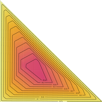
Figure 1: The optimal log-concave density $\hat{f}$ for the six data points in (4) with unit weights. The graph of the piecewise linear concave function $\log(\hat{f})$ is shown on the left. The regions of linearity are the seven triangles in the triangulation of the six points shown on the right.

Example 1.1.

Let $d=2$, $n=6$, $w=\frac{1}{6}(1,1,1,1,1,1)$, and fix the point configuration

$$X\,\,=\,\,\bigl{(}\,(0,0)\,,\,(100,0)\,,\,(0,100)\,,\,(22,37)\,,\,(43,22)\,,\,(36,41)\,\bigr{)}.$$ (4)

The graphical output generated by LogConcDEAD is shown on the left in Figure 1. This is the graph of the function ${\rm log}(\hat{f})$ that solves (3). This piecewise linear concave function has seven linear pieces, namely the triangles on the right in Figure 1, with vertices taken from $X$.

The purpose of this paper is to establish a link between nonparametric statistics and geometric combinatorics. We develop a generalization of the theory of regular triangulations arising in the context of maximum likelihood estimation for log-concave densities.

A key feature of our approach is that we emphasize the presence of unequal weights in the maximum likelihood estimation problem (3). In fact, it is important for us that the weights $w$ are allowed to vary. While this is a natural assumption from the perspective of geometry and combinatorics, it is also well-motived by statistics. For instance, unequal weights are necessary when applying the bootstrap to assess uncertainty in the density estimate. In addition, Leister [18, Section 2.3] studies Hidden Markov Models for state-dependent log-concave densities. Her EM algorithm solves the problem (3) repeatedly for different weights.

Our paper is organized as follows. In Section 2 we first review the relevant mathematical concepts, especially polyhedral subdivisions and secondary polytopes [9, 13]. We then generalize results in [7] from the case of unit weights $w=\frac{1}{n}(1,1,\ldots,1)$ to arbitrary weights $w$. Theorem 2.2 casts the problem (3) as a linear optimization problem over a convex subset $\mathcal{S}(X)$ of $\mathbb{R}^{n}$, which we call the Samworth body of $X$. Theorem 2.5 uses integrals as in [4] to give an unconstrained formulation of this problem with an explicit objective function.

Cule, Samworth and Stewart [7] discovered that log-concave density estimation leads to regular polyhedral subdivisions. In this paper we prove the following converse to their result:

Theorem 1.2.

Let $\Delta$ be any regular polyhedral subdivision of the configuration $X$. There exists a non-empty open subset $\,\mathcal{U}_{\Delta}$ in $\mathbb{R}^{n}$ such that, for every $w\in\mathcal{U}_{\Delta}$, the optimal solution $\hat{f}$ to (3) is a piecewise log-linear function whose regions of linearity are the cells of $\Delta$.

The proof of Theorem 1.2 appears in Section 3. We introduce a remarkable symmetric function $H$ that serves as a key technical tool. The theory behind $H$ seems interesting in its own right. In Theorem 3.7 we characterize the normal cone at any boundary point of the Samworth body. In other words, for a given concave piecewise log-linear function $f$, we determine the set of all weight vectors $w$ such that $f$ is the optimal solution in (3).

In Section 4 we view (3) as a parametric optimization problem, as either $w$ or $X$ vary. Variation of $w$ is explained by the geometry of the Samworth body. We explore empirically the probability that a given subdivision is optimal. We observe that triangulations are rare. Thus pictures like the triangulation in Figure 1 are exceptional and deserve special attention.

In Section 5 we focus our attention on the case of unit weights, and we examine the constraints this imposes on $\Delta$. Theorem 5.1 shows that triangulations never occur for $n=d+2$ points in $\mathbb{R}^{d}$ with unit weights. A converse to this result is established in Theorem 5.3.

Sections 4 and 5 conclude with several open problems. These suggest possible lines of inquiry for a future research theme that might be named Nonparametric Algebraic Statistics.

2 Geometric Combinatorics

We begin by reviewing concepts from geometric combinatorics, studied in detail in the books by De Loera, Rambau and Santos [9] and Gel’fand, Kapranov and Zelevinsky [13]. See Thomas [20, §7-8] for a first introduction. Let $X=(x_{1},\ldots,x_{n})$ be a configuration as before and $P={\rm conv}(X)$ its convex hull in $\mathbb{R}^{d}$. We assume that the polytope $P$ has dimension $d$.

Fix a real vector $y=(y_{1},\ldots,y_{n})$. We write $h_{X,y}$ for the smallest concave function $h$ on $\mathbb{R}^{n}$ such that $h(x_{i})\geq y_{i}$ for $i=1,\ldots,n$. The graph of $h_{X,y}$ is the upper convex hull of $\{(x_{1},y_{1}),\ldots,(x_{n},y_{n})\}$ in $\mathbb{R}^{n+1}$. Hence $h_{X,y}(t)$ is the largest real number $h^{*}$ such that $(t,h^{*})$ is in the convex hull of $\{(x_{1},y_{1}),\ldots,(x_{n},y_{n})\}$. In particular, $h_{X,y}(t)=-\infty$ for $t\not\in P$. Up to sign, the function $h_{X,y}$ is called the characteristic section in [9, Definition 5.2.12]. We also refer to $h_{X,y}$ as the tent function, with (some of) the points $(x_{i},y_{i})$ being the tent poles. The vector $y$ is called relevant if $h_{X,y}(x_{i})=y_{i}$ for $i=1,\ldots,n$, i.e. if each $(x_{i},y_{i})$ is a tent pole. This fails, for example, if $x_{i}$ lies in the interior of $P$ and $y_{i}$ is small relative to the other $y_{j}$.

A regular subdivision $\Delta$ of $X$ is a collection of subsets of $X$ whose convex hulls are the regions of linearity of the function $h_{X,y}$ for some $y\in\mathbb{R}^{n}$. These regions are $d$-dimensional polytopes, and are called the cells of $\Delta$. A regular subdivision $\Delta$ is a regular triangulation of $X$ if each cell is a $d$-dimensional simplex. The secondary polytope $\Sigma(X)$ is a polytope of dimension $n-d-1$ in $\mathbb{R}^{n}$ whose faces are in bijection with the regular subdivisions of $X$. In particular, the vertices of $\Sigma(X)$ correspond to the regular triangulations of $X$; see [9, §5].

If $\Delta$ is a regular triangulation of $X$, then the $k$-th coordinate of the corresponding vertex $z^{\Delta}$ of $\Sigma(X)\subset\mathbb{R}^{n}$ is the sum of the volumes of all simplices in $\Delta$ that contain $x_{k}$. In symbols,

$$z^{\Delta}_{k}\,\,=\,\,\sum_{\sigma\in\Delta:\atop x_{k}\in\sigma}{\rm vol}(\sigma).$$ (5)

We call $z^{\Delta}=(z^{\Delta}_{1},\ldots,z^{\Delta}_{n})$ the GKZ vector of the triangulation $\Delta$, in reference to [13].

The support function of the secondary polytope $\Sigma(X)$ is the piecewise linear function

$$\mathbb{R}^{n}\rightarrow\mathbb{R},\quad y\,\mapsto\,\int_{P}h_{X,y}(t)dt.$$

This follows from the equation in [9, page 232]. The function is linear on each cone in the secondary fan of $X$. For every $y$ in the secondary cone of a given regular triangulation $\Delta$,

$$\int_{P}h_{X,y}(t)dt\,\,=\,\,z^{\Delta}\cdot y\,\,=\,\,\sum_{i=1}^{n}z^{\Delta}_{i}y_{i}.$$ (6)

This means that the convex dual to the secondary polytope has the representation

$$\Sigma(X)^{*}\quad=\quad\bigl{\{}y\in\mathbb{R}^{n}\,:\,z^{\Delta}\cdot y\leq 1\,\,\hbox{for all}\,\,\Delta\bigr{\}}\,\,\,=\,\,\,\bigl{\{}y\in\mathbb{R}^{n}\,:\,\int_{P}h_{X,y}(t)dt\leq 1\,\bigr{\}}.$$

Note that $\Sigma(X)^{*}$ is an unbounded polyhedron in $\mathbb{R}^{n}$ since $\Sigma(X)$ has dimension $n-d-1$. Indeed, $\Sigma(X)^{*}$ is the product of an $(n-d-1)$-dimensional polytope and an orthant $\mathbb{R}_{\geq 0}^{d+1}$.

We now introduce an object that looks like a continuous analogue of $\Sigma(X)^{*}$. We define

$$\mathcal{S}(X)\quad=\quad\bigl{\{}\,y\in\mathbb{R}^{n}\,:\,\int_{P}{\rm exp}(h_{X,y}(t))dt\leq 1\,\bigr{\}}.$$ (7)

Inspired by [6, 7], we call $\mathcal{S}(X)$ the Samworth body of the point configuration $X$.

Proposition 2.1.

The Samworth body $\mathcal{S}(X)$ is a full-dimensional closed convex set in $\mathbb{R}^{n}$.

Proof.

Let $y,y^{\prime}\in\mathcal{S}(X)$ and consider a convex combination $y^{\prime\prime}=\alpha y+(1-\alpha)y^{\prime}$ where $0\leq\alpha\leq 1$. For all $t\in P$, we have $h_{X,y^{\prime\prime}}(t)\leq\alpha h_{X,y}(t)+(1-\alpha)h_{X,y^{\prime}}(t)$, and therefore

$${\rm exp}(h_{X,y^{\prime\prime}}(t))\,\leq\,{\rm exp}\bigl{(}\alpha h_{X,y}(t)+(1-\alpha)h_{X,y^{\prime}}(t)\bigr{)}\,\leq\,\alpha\cdot{\rm exp}(h_{X,y}(t))+(1-\alpha)\cdot{\rm exp}(h_{X,y^{\prime}}(t)).$$

Now integrate both sides of this inequality over all $t\in P$. The right hand side is bounded above by $1$, and hence so is the left hand side. This means that $y^{\prime\prime}\in\mathcal{S}(X)$. We conclude that $\mathcal{S}(X)$ is convex. It is closed because the defining function is continuous, and it is $n$-dimensional because all points $y$ whose $n$ coordinates are sufficiently negative lie in $\mathcal{S}(X)$. ∎

Every boundary point $y$ of the Samworth body $\mathcal{S}(X)$ defines a log-concave probability density function $f_{X,y}$ on $\mathbb{R}^{d}$ that is supported on the polytope $P={\rm conv}(X)$. This density is

$$f_{X,y}\,\,:\,\,\,t\,\,\mapsto\,\,\begin{cases}{\rm exp}(h_{X,y}(t))&{\rm if}\,\,\,t\in P,\\ \qquad 0&{\rm otherwise}.\end{cases}$$ (8)

We fix a positive real vector $w=(w_{1},\ldots,w_{n})\in\mathbb{R}^{n}_{\geq 0}$ that satisfies $\sum_{i=1}^{n}w_{i}=1$. The following result rephrases the key results of Cule, Samworth and Stewart [7, Theorems 2 and 3], who proved this, in a different language, for the unit weight case $w=\frac{1}{n}(1,1,\ldots,1)$.

Theorem 2.2.

The linear functional $\,y\mapsto w\cdot y=\sum_{i=1}^{n}w_{i}y_{i}$ is bounded above on the Samworth body $\,\mathcal{S}(X)$. Its maximum over $\,\mathcal{S}(X)\,$ is attained at a unique point $y^{*}$. The corresponding log-concave density $f_{X,y^{*}}$ is the unique optimal solution to the estimation problem (3).

Proof.

We are claiming that $\mathcal{S}(X)$ is strictly convex and its recession cone is contained in the negative orthant $\mathbb{R}^{n}_{\leq 0}$. The point $y^{*}$ represents the solution to the optimization problem

Maximize $$\,w\cdot y\, \,y\in\mathcal{S}(X)$$ subject to . (9)

The equivalence of (3) and (9) stems from the fact that the optimal solution $\hat{f}$ to the maximum likelihood problem (3) has the form $f=f_{X,y}$ for some choice of $y\in\mathbb{R}^{n}$. This was proven in [7] for unit weights $w=\frac{1}{n}(1,1,\ldots,1)$. The general case for positive weights $w\in\mathbb{R}^{n}$ follows analogously. To be precise, let $f$ be the maximum likelihood estimator for $(X,w)$, and let $y=\log(f(X))$ be the heights at the samples $X$. Then, the function $C\cdot f_{X,y}$, where $C\geq 1$ is the appropriate constant that makes the integral equal to $1$, gives a likelihood that is at least as large as $f$ does, with equality if and only if $f=f_{X,y}$. Thus, $f=f_{X,y}$.

Let $N$ be the sample size, so that $N_{i}=Nw_{i}$ is a positive integer for $i=1,\ldots,n$. We think of $x_{i}$ as a sample point in $\mathbb{R}^{d}$ that has been observed $N_{i}$ times. If $f$ is any probability density function on $\mathbb{R}^{d}$, then the log-likelihood of the $N$ observations with respect to $f$ equals

$$N\cdot\sum_{i=1}^{n}w_{i}\cdot{\rm log}(f(x_{i})).$$ (10)

Maximizing (10) over log-concave densities is equivalent to maximizing (2). We know from [7, Theorem 2] that the maximum is unique and is attained by $f=f_{X,y^{*}}$ for some $y^{*}\in\mathbb{R}^{n}$. Here $y^{*}$ is the unique relevant point in $\,\mathcal{S}(X)=\bigl{\{}y\in\mathbb{R}^{n}:\int_{\mathbb{R}^{d}}f_{X,y}(t)dt\leq 1\bigr{\}}\,$ that maximizes the linear functional $w\cdot y$. Hence (3) and (9) are equivalent for all $w\in\mathbb{R}^{n}_{\geq 0}$. ∎

The constrained optimization problem (9) can be reformulated as an unconstrained optimization problem. For the unit weight case $w_{1}=\cdots=w_{n}=1/n$, this was done in [7, §3.1]. This result can easily be extended to general weights. In the language of convex analysis, Proposition 2.3 says that the optimal value function of the convex optimization problem (9) is the Legendre-Fenchel transform of the convex function $y\mapsto\int_{P}{\rm exp}(h_{X,y}(t))dt$.

Proposition 2.3.

The constrained optimization problem (9) is equivalent to the unconstrained optimization problem

$$\hbox{{\rm Maximize} $\,\,w\cdot y-\int_{P}\exp(h_{X,y}(t))dt\,\,$ over all $\,\,y\in\mathbb{R}^{n}$},$$ (11)

where, as before, $P$ denotes the convex hull of $x_{1},\dots,x_{n}\in\mathbb{R}^{d}$ and $h_{X,y}$ is the tent function, i.e.,  $h_{X,y}:\mathbb{R}^{d}\to\mathbb{R}$ is the least concave function satisfying $h_{X,y}(x_{i})\geq y_{i}$ for all $i=1,\ldots,n$.

Proof.

A proof for uniform weights is given in [7]. We here present the proof for arbitrary weights $w_{1},\ldots,w_{n}$. These are positive real numbers that sum to $1$. This ensures that the objective function in (9) is bounded above, since the exponential term dominates when the coordinates of $y$ become large. Clearly, the optimum of (9) is attained on the boundary $\partial\mathcal{S}(X)$ of the feasible set $\mathcal{S}(X)$, and we could equivalently optimize over that boundary.

Now suppose that $y^{*}$ is an optimal solution of (11). This implies that $h_{X,y^{*}}(x_{i})=y^{*}_{i}$, i.e. each tent pole touches the tent. Otherwise $\,w\cdot y$ in the objective function can be increased without changing $\int_{P}\exp(h_{X,y}(t))dt$. Let $c:=\int_{P}\exp(h_{X,y^{*}}(t))dt$. We claim that $c=1$.

Let $\hat{y}$ be a vector in $\mathbb{R}^{n}$, also satisfying $h_{X,\hat{y}}(x_{i})=\hat{y}_{i}$ for all $i$, such that $\exp(h_{X,y^{*}}(t))=c\exp(h_{X,\hat{y}}(t))$ and $\int_{P}\exp(h_{X,\hat{y}}(t))dt=1$. This means that $h_{X,y^{*}}(t)=\log(c)+h_{X,\hat{y}}(t)$ for all points $t$ in the polytope $P$. In particular, we have $y_{i}^{*}-\hat{y}_{i}=\log(c)$ for $i=1,2,\ldots,n$.

We now analyze the difference of the objective functions at the points $\hat{y}$ and $y^{*}$:

$$w\cdot\hat{y}-\int_{P}\exp(h_{X,\hat{y}}(t))dt-\left(w\cdot y^{*}-\int_{P}\exp(h_{X,y^{*}}(t))dt\right)=-\log(c)-1+c.$$

Note that the function $c\mapsto-\log(c)-1+c$ is nonnegative. Since $y^{*}$ maximizes $w\cdot y-\int_{P}\exp(h_{X,y}(t))dt$, it follows that $-\log(c)-1+c=0$, which implies that $c=1$. So, the claim holds. We have shown that the solution $y^{*}$ of (11) also solves the following problem:

Maximize $$\,w\cdot y-\int_{P}\exp(h_{X,y}(t))dt \int_{P}\exp(h_{X,y}(t))dt=1$$   subject to  . (12)

But this is equivalent to the constrained formulation (9), and the proof is complete. ∎

The objective function in (11) looks complicated because of the integral and because $h_{X,y}(t)$ depends piecewise linearly on both $y$ and $t$. To solve our optimization problem, a more explicit form is needed. This was derived by Cule, Samworth and Stewart in [7, Section B.1]. The formula that follows writes the objective function locally as an exponential-rational function. This can also be derived from work on polyhedral residues due to Barvinok [4].

Lemma 2.4.

Fix a simplex $\sigma={\rm conv}(x_{0},x_{1},\ldots,x_{d})$ in $\mathbb{R}^{d}$ and an affine-linear function $\ell:\mathbb{R}^{d}\rightarrow\mathbb{R}$, and let $y_{0}=\ell(x_{0}),y_{1}=\ell(x_{1}),\ldots,y_{d}=\ell(x_{d})$ be its values at the vertices. Then

$$\int_{\sigma}{\rm exp}\bigl{(}\ell(t)\bigr{)}dt\,\,\,=\,\,\,{\rm vol}(\sigma)\cdot\sum_{i=0}^{d}{\rm exp}(y_{i})\!\!\prod_{j\in\{0,\ldots,d\}\backslash\{i\}}\!\!\!\!\!(y_{i}-y_{j})^{-1}.$$

Proof.

This follows directly from equation (B.1) in [7, Section B.1], and it can also easily be derived from Barvinok’s formula in [4, Theorem 2.6]. ∎

This lemma implies the following formula for integrating exponentials of piecewise-affine functions on a convex polytope. This can be regarded as an exponential variant of (6).

Theorem 2.5.

Let $\Delta$ be a triangulation of the configuration $X=(x_{1},\ldots,x_{n})$ and $h:P\rightarrow\mathbb{R}$ the piecewise-affine function on $\Delta$ that takes values $h(x_{i})=y_{i}$ for $i=1,2,\ldots,n$. Then

$$\int_{P}{\rm exp}\bigl{(}h(t)\bigr{)}dt\,\,\,=\,\,\,\sum_{i=1}^{n}{\rm exp}(y_{i})\sum_{\sigma\in\Delta:\atop i\in\sigma}\frac{{\rm vol}(\sigma)}{\prod_{j\in\sigma\backslash i}(y_{i}-y_{j})}$$

Proof.

We add the expressions in Lemma 2.4 over all maximal simplices $\sigma$ of the triangulation $\Delta$, and we collect the rational function multipliers for each of the $n$ exponentials ${\rm exp}(y_{i})$. ∎

This formula underlies the efficient solution to the estimation problem (3) that is implemented in the R package LogConcDEAD [6]. We record the following algebraic reformulation, which will be used in our study in the subsequent sections. This follows from Theorem 2.5.

Corollary 2.6.

The equivalent optimization problems (3), (9), (11) are also equivalent to

$${\rm Maximize}\,\,\,w\cdot y\,-\,\sum_{\sigma\in\Delta}\sum_{i\in\sigma}\frac{{\rm vol}(\sigma)\cdot{\rm exp}(y_{i})}{\prod_{j\in\sigma\backslash i}(y_{i}-y_{j})},$$ (13)

where $y$ runs over $\mathbb{R}^{n}$ and $\Delta$ is a regular triangulation of $X$ whose secondary cone contains $y$.

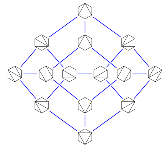
Figure 2: The associahedron is the secondary polytope for the six vertices of a hexagon. This diagram belongs to David Epstein. It was first appeared in his blog post [11] and it was published as Figure 15 in his article [12].

We close this section with an example that illustrates the various concepts seen so far.

Example 2.7.

Let $d=2$ and $n=6$. Take $X$ to be six points in convex position in the plane, labeled cyclically in counterclockwise order. The normalized area of the triangle formed by any three of the vertices of the hexagon $P={\rm conv}(X)$ is computed as a $3\times 3$-determinant

$$\quad v_{ijk}\,\,:=\,\,{\rm vol}\bigl{(}{\rm conv}(x_{i},x_{j},x_{k})\bigr{)}\,\,=\,\,{\rm det}\begin{pmatrix}1&1&1\\ x_{i}&x_{j}&x_{k}\end{pmatrix}\,\,\quad{\rm for}\,\,\,\,1\leq i<j<k\leq 6.\quad$$ (14)

The configuration $X$ has $14$ regular triangulations. These come in three symmetry classes: six triangulations like $\Delta=\{123,134,145,156\}$, six triangulations like $\,\Delta^{\prime}=\{123,134,146,456\}$, and two triangulations like $\,\Delta^{\prime\prime}=\{123,135,156,345\}$. The corresponding GKZ vectors are

$$\begin{matrix}z^{\Delta}&=&\bigl{(}\,v_{123}+v_{134}+v_{145}+v_{156}\,,\,v_{123}\,,\,v_{123}+v_{134}\,,\,v_{134}+v_{145}\,,\,v_{145}+v_{156}\,,v_{156}\,\bigr{)},\\ z^{\Delta^{\prime}}&=&\bigl{(}\,v_{123}+v_{134}+v_{146}\,,\,v_{123}\,,\,v_{123}+v_{134}\,,\,v_{134}+v_{146}+v_{456}\,,\,v_{456}\,,\,v_{146}+v_{456}\,\bigr{)},\\ z^{\Delta^{\prime}}&=&\bigl{(}\,v_{123}+v_{135}+v_{156}\,,\,v_{123}\,,\,v_{123}+v_{135}+v_{345}\,,\,v_{345}\,,\,v_{135}+v_{156}+v_{345}\,,\,v_{156}\,\bigr{)},\end{matrix}$$

as defined in (5). The secondary polytope $\Sigma(X)$ is the convex hull of these $14$ points in $\mathbb{R}^{6}$. This is a simple $3$-polytope with $14$ vertices, $21$ edges and $9$ facets, shown in Figure 2. This polytope is known as the associahedron. It has $45=14+21+9+1$ faces in total, one for each of the $45$ polyhedral subdivisions of $X$. These are the supports of the functions $h_{X,y}$.

For example, the edge of $\Sigma(X)$ that connects $z^{\Delta}$ and $z^{\Delta^{\prime}}$ represents the subdivision $\{123,134,1456\}$, with two triangles and one quadrangle. The smallest face containing $\{z^{\Delta},z^{\Delta^{\prime}},z^{\Delta^{\prime\prime}}\}$ is two-dimensional. It is a pentagon, encoding the subdivision $\{123,13456\}$.

The Samworth body $\mathcal{S}(X)$ is full-dimensional in $\mathbb{R}^{6}$. Its boundary is stratified into $45$ pieces, one for each subdivision of $X$. For any given $w\in\mathbb{R}^{6}$, the optimal solution $y^{*}$ to (9) lies in precisely one of these $45$ strata, depending on the shape of the optimal density $f_{X,y^{*}}$.

Algebraically, we can find $y^{*}$ by computing the maximum among $14$ expressions like

$$\begin{matrix}w_{1}y_{1}+w_{2}y_{2}+\cdots+w_{6}y_{6}&-&v_{123}\cdot\bigl{(}\frac{{\rm exp}(y_{1})}{(y_{1}-y_{2})(y_{1}-y_{3})}+\frac{{\rm exp}(y_{2})}{(y_{2}-y_{1})(y_{2}-y_{3})}+\frac{{\rm exp}(y_{3})}{(y_{3}-y_{1})(y_{3}-y_{2})}\bigr{)}\vskip 3.0pt plus 1.0pt minus 1.0pt\\ &-&v_{134}\cdot\bigl{(}\frac{{\rm exp}(y_{1})}{(y_{1}-y_{3})(y_{1}-y_{4})}+\frac{{\rm exp}(y_{3})}{(y_{3}-y_{1})(y_{3}-y_{4})}+\frac{{\rm exp}(y_{4})}{(y_{4}-y_{1})(y_{4}-y_{3})}\bigr{)}\vskip 3.0pt plus 1.0pt minus 1.0pt\\ &-&v_{145}\cdot\bigl{(}\frac{{\rm exp}(y_{1})}{(y_{1}-y_{4})(y_{1}-y_{5})}+\frac{{\rm exp}(y_{4})}{(y_{4}-y_{1})(y_{4}-y_{5})}+\frac{{\rm exp}(y_{5})}{(y_{5}-y_{1})(y_{5}-y_{4})}\bigr{)}\vskip 3.0pt plus 1.0pt minus 1.0pt\\ &-&v_{156}\cdot\bigl{(}\frac{{\rm exp}(y_{1})}{(y_{1}-y_{5})(y_{1}-y_{6})}+\frac{{\rm exp}(y_{5})}{(y_{5}-y_{1})(y_{5}-y_{6})}+\frac{{\rm exp}(y_{6})}{(y_{6}-y_{1})(y_{6}-y_{5})}\bigr{)}.\end{matrix}$$ (15)

This formula is the objective function in (13) for the triangulation $\Delta=\{123,134,145,156\}$. The mathematical properties of this optimization process will be studied in the next sections.

3 Every Regular Subdivision Arises

Our goal in this section is to prove Theorem 1.2. We begin by examining the function

$$H\,:\,\mathbb{R}^{d}\rightarrow\mathbb{R}\,,\,\,\,(u_{1},\ldots,u_{d})\,\,\mapsto\,\,(-1)^{d}\frac{1+u_{1}^{-1}+\cdots+u_{d}^{-1}}{u_{1}u_{2}\cdots u_{d}}\,+\,\sum_{j=1}^{d}\frac{e^{u_{j}}}{u_{j}^{2}\prod_{k\not=j}(u_{j}-u_{k})}.$$ (16)

Proposition 3.1.

The function $H$ is well-defined on $\mathbb{R}^{d}$. It admits the series expansion

$$H(u_{1},\dots,u_{d})\quad=\quad\sum_{r=0}^{\infty}\frac{h_{r}(u_{1},\ldots,u_{d})}{(r+d+1)!},$$ (17)

where $h_{r}$ is the complete homogeneous symmetric polynomial of degree $r$ in $d$ unknowns.

Proof.

We substitute the Taylor expansion of the exponential function in the sum on the right hand side of (16). This sum then becomes

$$\sum_{j=1}^{d}\frac{e^{u_{j}}}{u_{j}^{2}\prod_{k\not=j}(u_{j}-u_{k})}\quad=\quad\sum_{\ell=0}^{\infty}\frac{1}{\ell!}\sum_{j=1}^{d}\frac{u_{j}^{\ell-2}}{\prod_{k\not=j}(u_{j}-u_{k})}\quad$$

$$=\quad\sum_{\ell=0}^{\infty}\frac{1}{\ell!}\sum_{j=1}^{d}\frac{u_{j}^{\ell-d-1}}{\prod_{k\not=j}(1-u_{k}/u_{j})}\quad=\quad\sum_{r=-d-1}^{\infty}\frac{1}{(r+d+1)!}\sum_{j=1}^{d}\frac{u_{j}^{r}}{\prod_{k\not=j}(1-u_{k}/u_{j})}$$

For nonnegative values of the summation index $r=\ell-d-1$, the inner summand equals $h_{r}(u_{1},\ldots,u_{d})$, by Brion’s Theorem [19, Theorem 12.13]. For negative values of $r$, we use Ehrhart Reciprocity, in the form of [19, Lemma 12.15, eqn (12.7)], as seen in [19, Example 12.14]. The two terms for $r\in\{-d-1,-d\}$ cancel with the left summand on the right hand side of (16). The terms for $r\in\{-d+1,\ldots,-2,-1\}$ are zero. This implies (17). ∎

We shall derive a useful integral representation of our function $H$. What follows is a Lebesgue integral over the standard simplex $\,\Sigma_{d}=\{(y_{1},\dots,y_{d})\in\mathbb{R}^{d}:\,y_{i}\geq 0,\,\sum_{i}y_{i}\leq 1\}$.

Proposition 3.2.

The function $H$ can be expressed as the following integral:

$$H(u_{1},\ldots,u_{d})\,\,=\,\int_{\Sigma_{d}}\left(1-\sum_{i=1}^{d}t_{i}\right)\exp\left(\sum_{i=1}^{d}u_{i}t_{i}\right)\text{d}t_{1}\dots\text{d}t_{d}.$$ (18)

Proof.

The complete homogeneous symmetric polynomial $h_{r}$ equals the Schur polynomial $s_{(r)}$ corresponding to the partition $\lambda=(r)$. By formula (2.11) in [16] we have $s_{(r)}=Z_{(r)}$, where $Z_{\lambda}(u_{1},\dots,u_{d})$ is the zonal polynomial, or spherical function [16]. Therefore, we conclude

$$H(u_{1},\ldots,u_{d})\,=\,\sum_{r=0}^{\infty}\frac{Z_{(r)}(u_{1},\ldots,u_{d})}{(r+d+1)!}\,=\,\frac{1}{(d+1)!}\sum_{r=0}^{\infty}\frac{Z_{(r)}(u_{1},\ldots,u_{d})\cdot[1]_{(r)}}{[d+2]_{(r)}\cdot r!},$$

where $[a]_{\lambda}=\prod_{j=1}^{m}(a-j+1)_{\lambda_{j}}$ for a partition $\lambda=(\lambda_{1},\dots,\lambda_{m})$, and $(a)_{s}=a(a+1)\cdots(a+s-1)$. In particular, $[1]_{(r)}=r!$, and $[1]_{\lambda}=0$ if $\lambda$ has more than one nonzero part. Therefore,

$$H(u_{1},\ldots,u_{d})\,\,=\,\,\frac{1}{(d+1)!}\sum_{\text{all partitions }\lambda}\frac{Z_{\lambda}(u_{1},\ldots,u_{d})\cdot[1]_{\lambda}}{[d+2]_{\lambda}\cdot|\lambda|!}.$$

By [16, (4.14)], this can be written in terms of the confluent hypergeometric function of matrix argument ${}_{1}F_{1}$:

$$H(u_{1},\ldots,u_{d})\,\,=\,\,\frac{1}{(d+1)!}\cdot\,{}_{1}F_{1}(1;d+2;\mbox{diag}{(}u_{1},\ldots,u_{d})).$$

The right hand side has the desired integral representation (18), by [16, equation (5.14)]. ∎

Corollary 3.3.

The function $H$ is positive, increasing in each variable, and convex.

Proof.

The integrand in (18) is nonnegative. Hence, $H(u_{1},\ldots,u_{d})>0$ for all $(u_{1},\ldots,u_{d})\in\mathbb{R}^{d}$. After taking derivatives with respect to $u_{i}$, the integrand remains positive. Therefore, $H$ is increasing in $u_{i}$. Finally, the integrand is a convex function, and hence so is $H$. ∎

We now embark towards the proof of Theorem 1.2. Recall that a vector $y\in\mathbb{R}^{n}$ is relevant if $h_{X,y}(x_{i})=y_{i}$ for all $i$, i.e. the regular subdivision of $X$ induced by $y$ uses each point $x_{i}$.

Lemma 3.4.

Fix a configuration $X$ of $n$ points in $\mathbb{R}^{d}$. For any relevant $y^{*}\in\mathbb{R}^{n}$ that satisfies $\int_{\mathbb{R}^{d}}f_{X,y^{*}}(t)dt=1$, there are weights $w\in\mathbb{R}^{n}_{>0}$ such that $y^{*}$ is the optimal solution to (3)-(11).

Proof.

We use the formulation (13) which is equivalent to (3), (9), and (11). Let $\Delta$ be any regular triangulation that refines the regular subdivision given by $y$. In other words, we choose $\Delta$ so that (6) is maximized. The objective function in Corollary 2.6 takes the form

$$S(y_{1},\dots,y_{n})\,\,\,=\,\,\,w\cdot y-\sum_{i=1}^{n}\exp(y_{i})\sum_{\sigma\in\Delta,\atop i\in\sigma}\frac{\text{vol}(\sigma)}{\prod_{j\in\sigma\setminus i}(y_{i}-y_{j})}.$$

Consider the partial derivative of the objective function $S$ with respect to the unknown $y_{k}$:

$$\frac{\partial S}{\partial y_{k}}\,\,\,=\,\,\,w_{k}\,\,-\, \sum_{\sigma\in\Delta,\atop k\in\sigma}\text{vol}(\sigma)\exp(y_{k})\frac{1}{\prod_{j\in\sigma\setminus k}(y_{k}-y_{j})}\left(1-\sum_{j\in\sigma\setminus k}\frac{1}{(y_{k}-y_{j})}\right)$$

$$- \,\sum_{\sigma\in\Delta,\atop k\in\sigma}\text{vol}(\sigma)\sum_{j\in\sigma\setminus k}\exp(y_{j})\frac{1}{\prod_{i\in\sigma\setminus j}(y_{j}-y_{i})}\frac{1}{(y_{j}-y_{k})}.$$

Using the formula (16) for the symmetric function $H(u_{1},\ldots,u_{d})$, this can be rewritten as

$$\frac{\partial S}{\partial y_{k}}\,\,\,=\,\,\,w_{k}\,-\,\sum_{\sigma\in\Delta,\atop k\in\sigma}\text{vol}(\sigma)\exp(y_{k})H(\{y_{i}-y_{k}:i\in\sigma\backslash k\}).$$

We now consider the specific given vector $y^{*}\in\mathbb{R}^{n}$, and we use it to define

$$w_{k}\,\,=\,\,\sum_{\sigma\in\Delta,\atop k\in\sigma}\text{vol}(\sigma)\exp(y^{*}_{k})H(\{y^{*}_{i}-y^{*}_{k}:i\in\sigma\backslash k\}).$$ (19)

By Corollary 3.3, the vector $w=(w_{1},\ldots,w_{n})$ is well-defined and has positive coordinates. Consider now our estimation problem (3) for that $w\in\mathbb{R}^{n}_{>0}$. By construction, the gradient vector of $S$ vanishes at $y^{*}$. Furthermore, recall that the choice of the triangulation $\Delta$ was arbitrary, provided $\Delta$ refines the subdivision of $y$. This ensures that all subgradients of the objective function in (11) vanish. Since this function is strictly convex, as shown in [7], we conclude that the given $y^{*}$ is the unique optimal solution for the choice of weights in (19). ∎

We note that the function $H$ and Lemma 3.4 are quite interesting even in dimension one.

Example 3.5.

Let $d=1$. So, we here examine log-concave density estimation for $n$ samples $x_{1}<x_{2}<\cdots<x_{n}$ on the real line. The function we defined in (16) has the representations

$$H(u)\,\,=\,\,\frac{e^{u}-u-1}{u^{2}}\,\,=\,\,\int_{0}^{1}(1-y)e^{uy}dy\,\,=\,\,\frac{1}{2}+\frac{1}{6}u+\frac{1}{24}u^{2}+\frac{1}{120}u^{3}+\cdots.$$

A vector $y^{*}\in\mathbb{R}^{n}$ is relevant if and only if

$${\rm det}\begin{pmatrix}1&1&1\\ x_{i-1}&x_{i}&x_{i+1}\\ y^{*}_{i-1}&y^{*}_{i}&y^{*}_{i+1}\end{pmatrix}\,\leq\,0\,\,\quad\hbox{for}\quad i=2,3,\ldots,n-1.$$ (20)

The desired vector $w\in\mathbb{R}^{n}_{>0}$ is defined by the formula in (19). The $k$-th coordinate of $w$ is

$$w_{k}=\begin{cases}(x_{2}-x_{1})e^{y^{*}_{1}}H(y^{*}_{2}-y^{*}_{1})&{\rm if}\,\,k=1,\\ (x_{k}-x_{k-1})e^{y^{*}_{k}}H(y^{*}_{k-1}-y^{*}_{k})+(x_{k+1}-x_{k})e^{y^{*}_{k}}H(y^{*}_{k+1}-y^{*}_{k})&{\rm if}\,\,2\leq k\leq n-1,\\ (x_{n}-x_{n-1})e^{y^{*}_{n}}H(y^{*}_{n-1}-y^{*}_{n})&{\rm if}\,\,k=n.\end{cases}$$

If we now further assume that $f_{X,y^{*}}={\rm exp}(h_{X,y^{*}})$ is a density, i.e. $\int_{-\infty}^{\infty}f_{X,y^{*}}(t)dt=1$, then $f_{X,y^{*}}$ is the unique log-concave density that maximizes the likelihood function for $(X,w)$.

Example 3.6.

For $d=2$, our symmetric convex function $H$ has the form

$$H(u,v)\,=\,\frac{1}{uv}+\frac{1}{u^{2}v}+\frac{1}{uv^{2}}+\frac{e^{u}}{u^{2}(u{-}v)}+\frac{e^{v}}{v^{2}(v{-}u)}\,=\,\frac{1}{6}+\frac{1}{24}(u+v)+\frac{1}{120}(u^{2}+uv+v^{2})+\cdots.$$

For planar configurations $X$, we use this function to map each point $y^{*}$ in the boundary of the Samworth body $\mathcal{S}(X)$ to a hyperplane $w\in\partial\mathcal{S}(X)^{*}$ that is tangent to $\partial\mathcal{S}(X)$ at $y^{*}$.

The set of all vectors $w\in\mathbb{R}^{n}$ that lead to a desired optimal solution $y^{*}\in\partial\mathcal{S}(X)$ is a convex polyhedral cone in $\mathbb{R}^{n}$. The following theorem characterizes that convex cone.

Theorem 3.7.

Fix a vector $y^{*}\in\mathbb{R}^{n}$ that is relevant for $X$. Let $\Delta_{1},\Delta_{2},\ldots,\Delta_{m}$ be all the regular triangulations of $X$ that refine the subdivision of $X$ given by $y^{*}$, and let $w^{\Delta_{i}}\in\mathbb{R}^{n}_{>0}$ be the vector defined by (19) for $\Delta_{i}$. Then, a vector $w\in\mathbb{R}^{n}_{>0}$ lies in the convex cone that is spanned by $\,w^{\Delta_{1}},w^{\Delta_{2}},\ldots,w^{\Delta_{m}}\,$ if and only if $\,y^{*}$ is the optimal solution for (3),(9),(11),(13).

Proof.

This follows from the fact that the cone of subgradients at each $y^{*}$ is convex, and, the gradients for each triangulation on which $h_{X,y^{*}}$ is linear are also subgradients at $y^{*}$; cf. [7]. We can take any convex combination of these subgradients to obtain another subgradient. ∎

Example 3.8 ($n{=}4,d{=}2$).

Fix four points $x_{1},x_{2},x_{3},x_{4}$ in counterclockwise convex position in $\mathbb{R}^{2}$. These admit two regular triangulations, $\Delta_{1}=\{124,234\}$ and $\Delta_{2}=\{123,134\}$. Consider any $y\in\mathbb{R}^{4}$ with $\int_{\mathbb{R}^{2}}f_{X,y}(t)dt=1$. The vector $w^{\Delta_{1}}\in\mathbb{R}^{4}$ has coordinates

$$w_{1}^{\Delta_{1}} \,\,=\,\,v_{124}e^{y_{1}}H(y_{2}-y_{1},y_{4}-y_{1})$$

$$w_{2}^{\Delta_{1}} \,\,=\,\,v_{124}e^{y_{2}}H(y_{1}-y_{2},y_{4}-y_{2})+v_{234}e^{y_{2}}H(y_{3}-y_{2},y_{4}-y_{2})$$

$$w_{3}^{\Delta_{1}} \,\,=\,\,v_{234}e^{y_{3}}H(y_{2}-y_{3},y_{4}-y_{3})$$

$$w_{4}^{\Delta_{1}} \,\,=\,\,v_{124}e^{y_{4}}H(y_{1}-y_{4},y_{2}-y_{4})+v_{234}e^{y_{4}}H(y_{2}-y_{4},y_{3}-y_{4}).$$

Here $v_{ijk}$ denotes the triangle area in (14). Similarly, the vector $w^{\Delta_{2}}$ has coordinates

$$w_{1}^{\Delta_{2}} \,\,=\,\,v_{123}e^{y_{1}}H(y_{2}-y_{1},y_{3}-y_{1})+v_{134}e^{y_{1}}H(y_{3}-y_{1},y_{4}-y_{1})$$

$$w_{2}^{\Delta_{2}} \,\,=\,\,v_{123}e^{y_{2}}H(y_{1}-y_{2},y_{3}-y_{2})$$

$$w_{3}^{\Delta_{2}} \,\,=\,\,v_{123}e^{y_{3}}H(y_{1}-y_{3},y_{2}-y_{3})+v_{134}e^{y_{3}}H(y_{1}-y_{3},y_{4}-y_{3})$$

$$w_{4}^{\Delta_{2}} \,\,=\,\,v_{134}e^{y_{4}}H(y_{1}-y_{4},y_{3}-y_{4}).$$

In these formulas, the bivariate function $H$ can be evaluated as in Example 3.6.

We now distinguish three cases for $y$, depending on the sign of the $4\times 4$-determinant

$${\rm det}\begin{pmatrix}1&1&1&1\\ x_{1}&x_{2}&x_{3}&x_{4}\\ y_{1}&y_{2}&y_{3}&y_{4}\end{pmatrix}.$$ (21)

If (21) is positive then $y$ induces the triangulation $\Delta_{1}$. In that case, $y$ is the unique solution to our optimization problem whenever $w$ is any positive multiple of $w^{\Delta_{1}}$. If (21) is negative then $y$ induces $\Delta_{2}$ and it is the unique solution whenever $w$ is a positive multiple of $w^{\Delta_{2}}$. Finally, suppose (21) is zero, so $y$ induces the trivial subdivision $1234$. If $w$ is any vector in the cone spanned by $w^{\Delta_{1}}$ and $w^{\Delta_{2}}$ in $\mathbb{R}^{4}$ then $y$ is the optimal solution for (3),(9),(11),(13).

We next observe what happens in Theorem 3.7 when all coordinates of $y^{*}$ are equal.

Corollary 3.9.

Fix the constant vector $y^{*}=(c,c,\ldots,c)$, where $c=-{\rm log}({\rm vol}(P))$, so as to ensure that $\int_{\mathbb{R}^{d}}f_{X,y^{*}}(t)dt=1$. For any regular triangulation $\Delta_{i}$, the weight vector in (19) is a constant multiple of the GKZ vector in (5). More precisely, we have $w^{\Delta_{i}}=\frac{e^{c}}{(d+1)!}\cdot z^{\Delta_{i}}$. Hence $y^{*}$ is the optimal solution for any $w$ in the cone over the secondary polytope $\Sigma(X)$.

Proof.

The constant term of the series expansion in Proposition 3.1 equals

$$H(0,0,\ldots,0)\,\,=\,\,\frac{1}{(d+1)!}.$$

This implies that the sum in (19) simplifies to $\frac{e^{c}}{(d+1)!}$ times the sum in (5). The last statement follows from Theorem 3.7 because the cone over $\sigma(X)$ is spanned by all GKZ vectors $z^{\Delta}$. ∎

We shall now prove the result that was stated in the Introduction.

Proof of Theorem 1.2.

Let $\Delta_{1},\ldots,\Delta_{m}$ be all regular triangulations that refine a given subdivision $\Delta$. To underscore the dependence on $y$, we write $w^{\Delta_{i}}_{y}$ for the vector defined in (19). Let $\mathcal{C}_{\Delta}$ denote the secondary cone of $\Delta$. This is the normal cone to $\Sigma(X)$ at the face with vertices $z^{\Delta_{1}},\ldots,z^{\Delta_{m}}$. In particular, we have $\,\dim(\text{span}(z^{\Delta_{1}},\dots,z^{\Delta_{m}}))=n-\dim(\mathcal{C}_{\Delta})$.

For $y\in\mathbb{R}^{n}$ we abbreviate $N(y)=\dim(\text{span}(w^{\Delta_{1}}_{y},\dots,w^{\Delta_{m}}_{y}))$. The closure of the cone $\mathcal{C}_{\Delta}$ contains the constant vector $y^{0}=(c,c,\ldots,c)$, where $c=-{\rm log}({\rm vol}(P))$. Corollary 3.9 implies that $N(y_{0})=n-\dim(\mathcal{C}_{\Delta})$. The matrix $(w^{\Delta_{1}}_{y},\dots,w^{\Delta_{m}}_{y})$ depends analytically on the parameter $y$. Its rank is an upper semicontinuous function of $y$. Thus, there exists an open ball $\hat{\mathcal{B}}$ in $\mathbb{R}^{n}$ that contains $y_{0}$ and such that $N(y)\geq n-\dim(\mathcal{C}_{\Delta})$ for every $y\in\hat{\mathcal{B}}$. Now, let $\mathcal{B}=\mathcal{C}_{\Delta}\cap\hat{\mathcal{B}}$. The set $\mathcal{B}$ is full-dimensional in $\mathcal{C}_{\Delta}$, and $N(y)\geq n-\dim(\mathcal{C}_{\Delta})$ for all $y\in\mathcal{B}$.

For each $y\in\mathcal{B}$ we consider the convex cone in Theorem 3.7, which consists of all weight vectors $w$ for which the optimum occurs at $y$. We denote it by $\,{\rm cone}(w^{\Delta_{1}}_{y},\ldots,w^{\Delta_{m}}_{y})$. These convex cones are pairwise disjoint as $y$ runs over $\mathcal{B}$, and they depend analytically on $y$. Since the dimension of each cone is at least $n-{\rm dim}(\mathcal{B})$, it follows that the semi-analytic set

$$\bigcup_{y\in\mathcal{B}}{\rm cone}(w^{\Delta_{1}}_{y},\dots,w^{\Delta_{m}}_{y}).$$ (22)

is full-dimensional in $\mathbb{R}^{n}$. By Theorem 3.7, for each $w$ in the set (22), the optimal solution $\hat{f}$ to (3) is a piecewise log-linear function whose regions of linearity are the cells of $\Delta$. ∎

We conclude this section with the following open problem.

Problem 3.10.

Show that the rank $N(y)$ of the matrix $(w^{\Delta_{1}}_{y},\ldots,w^{\Delta_{m}}_{y})$ is the same for all vectors $y$ that induce the regular subdivision $\Delta$, namely we have $\,N(y)=n-{\rm dim}(\mathcal{C}_{\Delta})$.

For the proof of Theorem 1.2, it was sufficient to only have this constant-dimension property for all $y$ in a relatively open subset $\mathcal{B}$ of the secondary cone $\mathcal{C}_{\Delta}$. Problem 3.10 puts forth the conjecture that this property holds throughout the entire secondary cone $\mathcal{C}_{\Delta}$.

4 The Samworth Body

The maximum likelihood problem studied in this paper is a linear optimization problem over a convex set. We named that convex set the Samworth body, in recognition of the contributions made by Richard Samworth and his collaborators [6, 7]. In what follows we explore the geometry of the Samworth body. We begin with the following explicit formula:

Corollary 4.1.

The Samworth body of a given configuration $X$ of $\,n$ points in $\mathbb{R}^{d}$ equals

$$\!\mathcal{S}(X)\,\,=\,\,\biggl{\{}(y_{1},\ldots,y_{n})\in\mathbb{R}^{n}\,:\,\sum_{\sigma\in\Delta}\sum_{i\in\sigma}\frac{{\rm vol}(\sigma)\cdot{\rm exp}(y_{i})}{\prod_{j\in\sigma\backslash i}(y_{i}-y_{j})}\leq 1\,\,\,\hbox{for all $\Delta$ that refine $y\,$}\biggr{\}}.$$ (23)

This is a closed convex subset of $\,\mathbb{R}^{n}$. In the defining condition we mean that $\Delta$ runs over all regular triangulations that refine the regular polyhedral subdivision of $X$ specified by $y$.

Proof.

This is a reformulation of the definition (7) using the formulas in Theorem 2.5 and Corollary 2.6. Closedness and strict convexity of $\mathcal{S}(X)$ were noted in Theorem 2.2. ∎

Maximization of a linear function $w$ over $\mathcal{S}(X)$ becomes an unconstrained problem via the Legendre-Fenchel transform as in (13). By solving this problem for many instances of $w$, one can approximate the shape of $\mathcal{S}(X)$. Indeed, each regular subdivision of $X$ specifies a full-dimensional subset in the boundary of the dual body $\mathcal{S}(X)^{*}$, by Theorem 1.2. If we choose a direction $w$ at random in $\mathbb{R}^{n}$, then a unique positive multiple $\lambda w$ lies in $\partial\mathcal{S}(X)^{*}$, in the stratum associated to the subdivision of $X$ specified by the optimal solution $y^{*}\in\partial\mathcal{S}(X)$. By evaluating the map $w\mapsto y^{*}$ many times, we thus obtain the empirical distribution on the subdivisions, indicating the proportion of volumes of the strata in $\partial\mathcal{S}(X)^{*}$. In the next example we compute this distribution when the double sum in (23) looks like that in (15).

Example 4.2.

Let $d=2$, $n=6$, and take our configuration $X$ to be the six points $(0,0),(1,0),(2,1),(2,2),(1,2),(0,1)$. We sampled 100,000 vectors $w$ uniformly from the simplex $\{w\in\mathbb{R}^{6}_{\geq 0}:\sum_{i=1}^{6}w_{i}=1\}$. For each $w$, we computed the optimal $y^{*}\in\mathbb{R}^{6}$, and we recorded the subdivision of $X$ that is the support of $h_{X,y^{*}}$. We know from Example 2.7 that the secondary polytope $\Sigma(X)$ is an associahedron, which has $14+21+9+1=45$ faces. We here code each subdivision by a list of length $3,2,1$ or $0$ from among the diagonal segments

$$13,\,14,\,15,\,24,\,25,\,26,\,35,\,36,\,46.$$

For instance, the list $13\,\,14\,\,15$ encodes the triangulation $\Delta$ in Example 2.7. The edge connecting the triangulations $\Delta$ and $\Delta^{\prime}$ from Example 2.7 is denoted $13\,14$. We write $\emptyset$ for the trivial flat subdivision. The following table of percentages shows the empirical distribution we observed for the $45$ outcomes of our experiment:

$$\begin{matrix}\emptyset&35\,&\,46\,&\,24\,&\,15\,&\,13\,&\,26\,&\,25\,&\,14\,&\,36\\ 30.5\,\,&\,\,5.95\,\,&\,\,5.85\,\,&\,\,5.84\,\,&\,\,5.83\,\,&\,\,5.75\,\,&\,\,5.70\,\,&\,\,3.91\,\,&\,\,3.90\,\,&\,\,3.87\\ \end{matrix}$$

$$\setcounter{MaxMatrixCols}{13}\begin{matrix}13\,15&26\,46&15\,35&13\,35&24\,26&24\,46&13\,14&35\,36&14\,24&26\,36&14\,46&25\,35&15\,25\\ 1.23&1.21&1.21&1.20&1.16&1.14&0.96&0.92&0.92&0.92&0.92&0.90&0.90\end{matrix}$$

$$\setcounter{MaxMatrixCols}{12}\begin{matrix}25\,26&14\,15&36\,46&24\,25&13\,36&13\,46&26\,35&15\,24&13\,14\,15&13\,15\,35&14\,24\,46&24\,26\,46\\ 0.89&0.89&0.87&0.87&0.84&0.82&0.77&0.70&0.25&0.24&0.23&0.22\end{matrix}$$

$$\begin{matrix}15\,25\,35&26\,36\,46&13\,35\,36&24\,25\,26&13\,36\,46&25\,26\,35&15\,24\,25&14\,15\,24&13\,14\,46&26\,35\,36\\ 0.22&0.21&0.20&0.18&0.18&0.16&0.15&0.15&0.15&0.14\end{matrix}$$

The entry marked $\emptyset$ reveals that the trivial subdivision occurs with the highest frequency. This means that a large portion of the dual boundary $\partial\mathcal{S}(X)^{*}$ is flat. Equivalently, the Samworth body $\mathcal{S}(X)$ has a “very sharp edge” along the lineality space of the secondary fan.

To get a better understanding of the geometry of the Samworth body $\mathcal{S}(X)$, at least when $d$ or $n-d$ are small, we can also use the algebraic formula in (23) for explicit computations.

Example 4.3.

Let $d=3$, $n=6$, and fix the configuration of vertices of a regular octahedron:

$$X\,=\,(x_{1},x_{2},\ldots,x_{6})\,=\,\bigl{(}\,+e_{1}\,,\,-e_{1}\,,\,\,+e_{2},\,-e_{2}\,,\,\,+e_{3}\,,\,-e_{3}\,\bigr{)}.$$

Here $e_{i}$ denotes the $i$th unit vector in $\mathbb{R}^{3}$. The secondary polytope $\Sigma(X)$ is a triangle. Its edges correspond to the three subdivisions of the octahedron $X$ into two square-based pyramids, $\Delta_{1234}=\{12345,12346\}$, $\Delta_{1256}=\{12356,12456\}$, and $\Delta_{3456}=\{13456,23456\}$. Its vertices correspond to the three triangulations of $X$, namely $\Delta_{12}=\{1235,1236,1245,1256\}$, $\Delta_{34}=\{1345,1346,2345,2346\}$, and $\Delta_{56}=\{1356,1456,2356,2456\}$.

The normal fan of $\Sigma(X)$, which is the secondary fan of $X$, has three full-dimensional cones in $\mathbb{R}^{6}$. A vector $y$ in $\mathbb{R}^{6}$ selects the triangulation $\Delta_{ij}$ if $y_{i}+y_{j}$ is the uniquely attained minimum among $\{y_{1}+y_{2},\,y_{3}+y_{4},\,y_{5}+y_{6}\}$. It selects $\Delta_{1234}$ if $y_{1}+y_{2}=y_{3}+y_{4}<y_{5}+y_{6}$, and it leaves the octahedron unsubdivided when $y$ is in the lineality space $\,\{y\in\mathbb{R}^{6}:y_{1}+y_{2}=y_{3}+y_{4}=y_{5}+y_{6}\}$.

The Samworth body $\mathcal{S}(X)$ is defined in $\mathbb{R}^{6}$ by the following system of three inequalities. Use the $i$th inequality when the $i$th number in the list $(y_{1}{+}y_{2},y_{3}{+}y_{4},y_{5}{+}y_{6})$ is the smallest:

$$\begin{matrix}\frac{e^{y_{1}}(2y_{1}-y_{6}-y_{5})(2y_{1}-y_{4}-y_{3})}{(y_{1}{-}y_{2})(y_{1}{-}y_{3})(y_{1}{-}y_{5})(y_{1}{-}y_{6})(y_{1}{-}y_{4})}-\frac{e^{y_{2}}(2y_{2}-y_{6}-y_{5})(2y_{2}-y_{4}-y_{3})}{(y_{1}{-}y_{2})(y_{2}{-}y_{3})(y_{2}{-}y_{5})(y_{2}{-}y_{6})(y_{2}{-}y_{4})}+\frac{e^{y_{3}}(2y_{3}-y_{6}-y_{5})}{(y_{1}{-}y_{3})(y_{2}{-}y_{3})(y_{3}{-}y_{5})(y_{3}{-}y_{6})}\vskip 3.0pt plus 1.0pt minus 1.0pt\\ \,\,+\frac{e^{y_{4}}(2y_{4}-y_{6}-y_{5})}{(y_{1}{-}y_{4})(y_{2}{-}y_{4})(y_{4}{-}y_{5})(y_{4}{-}y_{6})}-\frac{e^{y_{5}}(y_{4}-2y_{5}+y_{3})}{(y_{1}{-}y_{5})(y_{2}{-}y_{5})(y_{3}{-}y_{5})(y_{4}{-}y_{5})}-\frac{e^{y_{6}}(y_{4}-2y_{6}+y_{3})}{(y_{1}{-}y_{6})(y_{2}{-}y_{6})(y_{3}{-}y_{6})(y_{4}{-}y_{6})}\,\,\leq\,1\vskip 3.0pt plus 1.0pt minus 1.0pt\end{matrix}$$

$$\begin{matrix}\frac{e^{y_{1}}(2y_{1}-y_{6}-y_{5})}{(y_{1}-y_{3})(y_{1}-y_{4})(y_{1}-y_{5})(y_{1}-y_{6})}+\frac{e^{y_{2}}(2y_{2}-y_{6}-y_{5})}{(y_{2}-y_{3})(y_{2}-y_{4})(y_{2}-y_{5})(y_{2}-y_{6})}-\frac{e^{y_{3}}(2y_{3}-y_{6}-y_{5})(y_{2}-2y_{3}+y_{1})}{(y_{1}-y_{3})(y_{3}-y_{4})(y_{3}-y_{5})(y_{3}-y_{6})(y_{2}-y_{3})}\vskip 3.0pt plus 1.0pt minus 1.0pt\\ +\frac{e^{y_{4}}(2y_{4}-y_{6}-y_{5})(-2y_{4}+y_{1}+y_{2})}{(y_{1}-y_{4})(y_{3}-y_{4})(y_{4}-y_{5})(y_{4}-y_{6})(y_{2}-y_{4})}-\frac{e^{y_{5}}(y_{2}-2y_{5}+y_{1})}{(y_{1}-y_{5})(y_{2}-y_{5})(y_{3}-y_{5})(y_{4}-y_{5})}-\frac{e^{y_{6}}(y_{2}-2y_{6}+y_{1})}{(y_{1}-y_{6})(y_{2}-y_{6})(y_{3}-y_{6})(y_{4}-y_{6})}\,\,\leq\,1\vskip 3.0pt plus 1.0pt minus 1.0pt\end{matrix}$$

$$\!\begin{matrix}\frac{e^{y_{1}}(2y_{1}-y_{4}-y_{3})}{(y_{1}-y_{3})(y_{1}-y_{4})(y_{1}-y_{5})(y_{1}-y_{6})}+\frac{e^{y_{2}}(2y_{2}-y_{4}-y_{3})}{(y_{2}-y_{3})(y_{2}-y_{4})(y_{2}-y_{5})(y_{2}-y_{6})}-\frac{e^{y_{3}}(y_{2}-2y_{3}+y_{1})}{(y_{1}-y_{3})(y_{2}-y_{3})(y_{3}-y_{5})(y_{3}-y_{6})}-\vskip 3.0pt plus 1.0pt minus 1.0pt\\ \frac{e^{y_{4}}(-2y_{4}+y_{1}+y_{2})}{(y_{1}-y_{4})(y_{2}-y_{4})(y_{4}-y_{5})(y_{4}-y_{6})}{+}\frac{e^{y_{5}}(y_{4}-2y_{5}+y_{3})(y_{2}-2y_{5}+y_{1})}{(y_{1}-y_{5})(y_{3}-y_{5})(y_{5}-y_{6})(y_{4}-y_{5})(y_{2}-y_{5})}{-}\frac{e^{y_{6}}(y_{4}-2y_{6}+y_{3})(y_{2}-2y_{6}+y_{1})}{(y_{1}-y_{6})(y_{3}-y_{6})(y_{5}-y_{6})(y_{4}-y_{6})(y_{2}-y_{6})}\leq 1\vskip 3.0pt plus 1.0pt minus 1.0pt\end{matrix}$$

The dual convex body $\mathcal{S}(X)^{*}$ has seven strata of faces in its boundary: a $3$-dimensional manifold of $2$-dimensional faces, corresponding to the trivial subdivision, three $4$-dimensional manifolds of edges corresponding to $\Delta_{1234},\Delta_{1256},\Delta_{3456}$, and three $5$-dimensional manifolds of extreme points, corresponding to $\Delta_{12},\Delta_{34},\Delta_{56}$. Each $2$-dimensional face of $\mathcal{S}(X)^{*}$ is a triangle, like the secondary polytope $\Sigma(X)$. The dual to this convex set is the Samworth body $\mathcal{S}(X)$, which is strictly convex. Its boundary is singular along three $4$-dimensional strata are formed when two of the three inequalities above are active. These meet in a highly singular $3$-dimensional stratum which is formed when all three inequalities are active. These singularities of $\partial\mathcal{S}(X)$ exhibit the secondary fan of $X$. It is instructive to draw a cartoon, in dimension two or three, to visualize the boundary features of $\mathcal{S}(X)$ and $\mathcal{S}(X)^{*}$.

Up until this point, the premise of this paper has been that the configuration $X$ is fixed but the weights $w$ vary. Example 4.3 was meant to give an impression of the corresponding geometry, by describing in an intuitive language how a Samworth body $\mathcal{S}(X)$ can look like.

However, our premise is at odds with the perspective of statistics. For a statistician, the natural setting is to fix unit weights, $w=\frac{1}{n}(1,1,\ldots,1)$, and to assume that $X$ consists of $n$ points that have been sampled from some underlying distribution. Here, one cares about one distinguished point in $\partial\mathcal{S}(X)$ and less about the global geometry of the Samworth body. Specifically, we wish to know which face of $\mathcal{S}(X)^{*}$ is pierced by the ray $\bigl{\{}(\lambda,\ldots,\lambda)\,:\,\lambda\geq 0\bigr{\}}$.

Subdivision: number of				Convex	Gaussian	Uniform	Circular	Circular
3-gons	4-gons	5-gons	6-gons	hull	$\mathcal{N}(0,1)$	$a=0.5$	$a=0.3$	$a=0.1$
1	0	0	0	3	948	533	257	34
0	1	0	0	4	8781	6719	4596	1507
0	0	1	0	5	8209	9743	10554	8504
0	0	0	1	6	1475	2805	4495	9887
2	0	0	0	4	8	3	6	7
1	1	0	0	5	1	2	1	2
3	0	0	0	3	6	2	2	1
2	1	0	0	4	39	16	4	7
2	0	1	0	5	1	1	0	1
1	2	0	0	5	1	0	1	6
4	0	0	0	4	1	0	0	0
3	1	0	0	3	114	38	10	1
3	0	1	0	4	39	20	9	2
2	2	0	0	4	59	19	16	9
5	0	0	0	3	3	0	0	0
4	1	0	0	4	1	0	0	0
4	0	1	0	3	90	27	8	1
3	2	0	0	3	120	32	11	0
5	1	0	0	3	50	11	3	0
7	0	0	0	3	2	1	0	0

Table 1: The optimal subdivisions for six random points in the plane

Example 4.4.

Let $d=2$ and $n=6$ as in Example 4.2, but now with unit weights $w=\frac{1}{6}(1,1,1,1,1,1)$. We sample i.i.d. points $x_{1},\ldots,x_{6}$ from various distributions $f$ on $\mathbb{R}^{2}$, some log-concave and others not, and we compare the resulting maximum likelihood densities $\hat{f}$.

In what follows, we analyze the case where $f$ is a standard Gaussian distribution or a uniform distribution on the unit disc, and we contrast this to distributions of the form $X=(U_{1}^{a}\cos(2\pi U_{2}),U_{1}^{a}\sin(2\pi U_{2}))$, where $U_{1}$ and $U_{2}$ are independent uniformly distributed on the interval $[0,1]$ and $a<0.5$. Such distributions have more mass towards the exterior of the unit disc and are hence not log-concave. For $a=0.5$ this is the uniform distribution on the unit disc. We drew 20,000 samples $X=(x_{1},\ldots,x_{6})$ from each of these four distributions.

For each experiment, we recorded the number of vertices of the convex hull of the sample, we computed the optimal subdivision using LogConcDEAD, and we recorded the shapes of its cells. Our results are reported in Table 1. Each of the four right-most columns shows the number of experiments out of 20,000 that resulted in a subdivision as described in the five left-most columns. These columns do not add up to 20,000, because we discarded all experiments for which the optimization procedure did not converge due to numerical instabilities.

In the vast majority of cases, reported in the first four rows, the optimal solution $\hat{f}$ is log-linear. Here the subdivision is trivial, with only one cell. For instance, the fourth row is the 30.5% case in Example 4.2. In the last row, ${\rm conv}(X)$ is a triangle and the subdivision is a triangulation that uses all three interior points. We saw such a triangulation in Example 1.1. In fact, we constructed the data (4) by modifying one of the examples with seven cells found by sampling from a Gaussian $\mathcal{N}(0,1)$ distribution. Note that the subdivisions resulting from Gaussian samples tend to have more cells than those from other distributions.

The examples in this section illustrate two different interpretations of the data set $(X,w)$: either the configuration $X$ is fixed and the weight vector $w$ varies, or $w$ is fixed and $X$ varies. These are two different parametric versions of our optimization problem (3), (9), (11), (13). This generalizes the interpretation of the secondary polytope $\Sigma(X)$ seen in [9, Section 1.2], namely as a geometric model for parametric linear programming. The vertices of $\Sigma(X)$ represent the various collections of optimal bases when the matrix $X$ is fixed and the cost function $w$ varies. See [9, Exercise 1.17] for the case $d=2,n=6$, as in Examples 2.7, 4.2 and 4.4. Of course, it is very interesting to examine what happens when both $X$ and $w$ vary, and to study $\Sigma(X)$ as a function on the space of configurations $X$. This was done in [8]. The same problem is even more intriguing in the statistical setting introduced in this paper.

Problem 4.5.

Study the Samworth body as a function $X\mapsto\mathcal{S}(X)$ on the space of configurations. Understand log-concave density estimation as a parametric optimization problem.

This problem has many angles, aspects and subproblems. Here is one of them:

Problem 4.6.

For fixed $w$ and a fixed combinatorial type of subdivision $\Delta$, study the semi-analytic set of all configurations $X$ such that $\Delta$ is the optimal subdivision for the data $(X,w)$.

For instance, suppose we fix the triangulation $\Delta$ seen on the right of Figure 1. How much can we perturb the configuration in (4) and retain that $\Delta$ is optimal for unit weights? For $n{=}6,d{=}2$, give inequalities that characterize the space of all datasets $(X,w)$ that select $\Delta$.

An ultimate goal of our geometric approach is the design of new tools for nonparametric statistics. One aim is the development of test statistics for assessing whether a given sample comes from a log-concave distribution. Such tests are important, e.g. in economics [2, 3].

Problem 4.7.

Improve the accuracy of existing test statistics for log-concavityy [5, 17] by augmenting these with combinatorial properties (such as the f-vector) of the observed subdivision $\Delta$.

The idea is that $\Delta$ is likely to have more cells when $X$ is sampled from a log-concave distribution. Hence we might use the f-vector of $\Delta$ as a test statistic for log-concavity. The study of such tests seems related to the approximation theory of convex bodies developed by Adiprasito, Nevo and Samper [1]. What does their “higher chordality” mean for statistics?

5 Unit Weights

In this section we offer an analysis of the uniform weights case. Example 4.4 suggests that the flat subdivision occurs with overwhelming probability when the sample size is small. Our main result in this section establishes this flatness for the smallest non-trivial case $n=d+2$:

Theorem 5.1.

Let $X$ be a configuration of $n=d+2$ points that affinely span $\mathbb{R}^{d}$. For $w=\frac{1}{n}(1,\ldots,1)$, the optimal density $\hat{f}$ is log-linear, so the optimal subdivision of $X$ is trivial.

We shall use the following lemma, which can be derived by a direct computation.

Lemma 5.2.

The symmetric function $H$ in Section 4 satisfies the differential equation

$$\frac{\partial H}{\partial x_{1}}(x_{1},\dots,x_{d})\quad=\quad\frac{e^{x_{1}}H(-x_{1},x_{2}-x_{1},\dots,x_{d}-x_{1})-H(x_{1},\dots,x_{d})}{x_{1}}.$$

Proof of Theorem 5.1.

Our $d+2$ points in $\mathbb{R}^{d}$ can be partitioned uniquely into two affinely independent subsets whose convex hulls intersect. This gives rise to a unique identity

$$\sum_{i=1}^{k}\alpha_{i}x_{i}\,\,\,=\,\,\sum_{j=k+1}^{d+2}\beta_{j}x_{j},$$

where $1\leq k\leq d+1,\,\,\alpha_{1},\dots,\alpha_{k},\beta_{k+1},\dots,\beta_{d+2}\geq 0$, and $\sum\alpha_{i}=\sum\beta_{j}=1$. We abbreviate $\mathcal{D}=\{1,2,\ldots,d+2\}$. There are precisely three regular subdivisions of the configuration $X$:

1. the triangulation $\,\bigl{\{}\mathcal{D}\backslash\{1\},\mathcal{D}\backslash\{2\},\ldots,\mathcal{D}\backslash\{k\}\bigr{\}}$,

2. the triangulation $\,\bigl{\{}\mathcal{D}\backslash\{k{+}1\},\mathcal{D}\backslash\{k{+}2\},\ldots,\mathcal{D}\backslash\{d{+}2\}\bigr{\}}$,

3. the flat subdivision $\bigl{\{}\mathcal{D}\bigr{\}}$.

The simplex volumes $\,\sigma_{\mathcal{D}\setminus i}={\rm vol}\bigl{(}{\rm conv}(\,x_{\ell}:\ell\in\mathcal{D}\backslash\{i\})\bigr{)}\,$ satisfy the identity

$$\qquad\quad\sum_{i=1}^{k}\sigma_{\mathcal{D}\setminus i}\,\,\,=\,\,\sum_{j=k+1}^{d+2}\!\sigma_{\mathcal{D}\setminus j}\quad=\quad{\rm vol}({\rm conv}(X)).$$ (24)

Now let $w\in\mathbb{R}^{d+2}$ be a positive weight vector, and suppose that the optimal heights $y_{1},\dots,y_{d+2}$ do not induce the flat subdivision (iii). This means that the optimal subdivision is one of the triangulations (i) and (ii). We will show that in that case $w\not=(\lambda,\lambda,\ldots,\lambda)$.

After relabeling we may assume that (ii) is the optimal triangulation for the given weights $w$. This is equivalent to the inequality

$$\sum_{i=1}^{k}y_{i}\sigma_{\mathcal{D}\setminus i}\,\,\,>\,\,\sum_{j=k+1}^{d+2}y_{j}\sigma_{\mathcal{D}\setminus j}.\quad\qquad$$

In light of (24), at least one of $y_{1},\dots,y_{k}$ has to be larger than at least one of $y_{k+1},\dots,y_{d+2}$. After relabeling once more, we may assume that $\,y_{1}>y_{k+1}$.

Theorem 3.7 states that the weight vector $w$ is uniquely determined (up to scaling) by the optimal height vector $y$. Namely, the coordinates of $w$ are given by the formula (19) for the optimal triangulation (ii). That formula gives

$$w_{1}\,\,\,=\,\,\sum_{j=k+1}^{d+2}\sigma_{\mathcal{D}\backslash j}e^{y_{1}}H\bigl{(}y_{\ell}-y_{1}:\ell\in\mathcal{D}\backslash\{1,j\}\bigr{)},\quad$$ (25)

and

$$w_{k+1}\,\,\,=\,\,\sum_{j=k+2}^{d+2}\sigma_{\mathcal{D}\backslash j}e^{y_{k+1}}H\bigl{(}y_{\ell}-y_{k+1}:\ell\in\mathcal{D}\backslash\{k{+}1,j\}\bigr{)}.$$ (26)

For any index $j\in\{k{+}2,\dots,d{+}2\}$ we consider the expression

$$e^{y_{1}}H(y_{\ell}-y_{1}:\ell\in\mathcal{D}\backslash j)\,\,-\,\,e^{y_{k+1}}H(y_{\ell}-y_{k+1}:\ell\in\mathcal{D}\backslash j)\,\,$$ (27)

$$=\,\,\,\bigl{(}\,e^{y_{1}-y_{k+1}}H(y_{\ell}-y_{k+1}-(y_{1}-y_{k+1}):\ell\in\mathcal{D}\backslash j)\,-\,H(y_{\ell}-y_{k+1}:\ell\in\mathcal{D}\backslash j)\,\bigr{)}.$$

If we divide the parenthesized difference by $x_{1}=y_{1}-y_{k+1}$, then we obtain an expression as in the right hand side of Lemma 5.2. Then, by Lemma 5.2, the expression in (27) becomes

$$e^{y_{k+1}}\cdot(y_{1}-y_{k+1})\cdot\frac{\partial H}{\partial x_{1}}\bigl{(}\,y_{\ell}-y_{k+1}:\ell\in\mathcal{D}\backslash j\,\bigr{)}.$$

By Corollary 3.3, all partial derivatives of $H$ are positive. Also, recall that $y_{1}>y_{k+1}$. Therefore, the expression in (27) is positive. Hence, for any $j\in\{k{+}2,\dots,d{+}2\}$, we have

$$e^{y_{1}}H(y_{\ell}-y_{1}:\ell\in\mathcal{D}\backslash j)\,\,\,>\,\,\,e^{y_{k+1}}H(y_{\ell}-y_{k+1}:\ell\in\mathcal{D}\backslash j).$$

In the left expression it suffices to take $\,\ell\in\mathcal{D}\backslash\{1,j\}$, and in the right expression it suffices to take $\,\ell\in\mathcal{D}\backslash\{k{+}1,j\}$. Summing over all $j$, the identities (24), (25) and (26) now imply

$$w_{1}\,\,>\,\,w_{k+1}.$$

This means that $w\not=(\lambda,\lambda,\ldots,\lambda)$ for all $\lambda>0$. We conclude that it is impossible to get a nontrivial subdivision of $X$ as the optimal solution when all the weights are equal. ∎

We now show that the result of Theorem 5.1 is the best possible in the following sense.

Theorem 5.3.

For any integer $d\geq 2$, there exists a configuration of $n=d+3$ points in $\mathbb{R}^{d}$ for which the optimal subdivision with respect to unit weights is non-trivial.

The hypothesis $d\geq 2$ is essential in this theorem. Indeed, for $d=1$ it can be shown, using the formulas in Example 3.5, that the flat subdivision is optimal for any configuration of $d+3=4$ points on the line $\mathbb{R}$ with unit weights. Here is an illustration of Theorem 5.3.

         

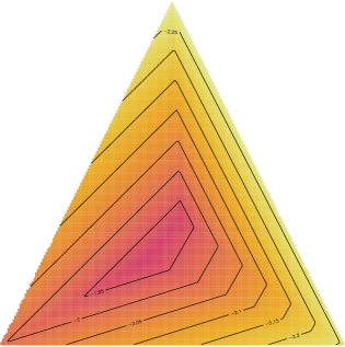
Figure 3: The optimal log-concave density for the five data points in (28) with unit weights.

Example 5.4.

Fix unit weights on the following five points in the plane:

$$X\,\,=\,\,\bigl{(}\,(0,0),\,(40,0),\,(20,40),\,(17,10),\,(21,15)\,\bigr{)}.$$ (28)

Using LogConcDEAD [6], we find that the optimal subdivision equals $\{124,245,235,1345\}$.

To derive Theorem 5.3, we first study the following configuration of $d+2$ points in $\mathbb{R}^{d}$:

$$X\,\,=\,\,\biggl{(}e_{1}\,,\,e_{2}\,,\,\ldots\,,\,e_{d}\,,\,0\,,\,\,\frac{1}{d+1}\sum_{i=1}^{d}e_{i}\,\biggr{)}.$$ (29)

Lemma 5.5.

Let $\alpha>0$ and assign weights as follows to the configuration $X$ in (29):

$$w_{1}=w_{2}=\cdots=w_{d+1}>0,\text{ and }\,\,w_{d+2}\,=\,w_{1}\frac{(d+1)e^{\alpha}H(-\alpha,-\alpha,\dots,-\alpha)}{dH(\alpha,0,\dots,0)}.$$ (30)

Then the optimal heights satisfy $\,y_{1}=y_{2}=\cdots=y_{d+1}\,$ and $\,y_{d+2}=y_{1}+\alpha$.

Proof.

Let $\mathcal{D}=\{1,\dots,d+2\}$ and fix $w$ as in (30). The volumes $\text{vol}(\mathcal{D}\backslash\{i\})$ are equal for $i\in\{1,\dots,d+1\}$. Set $\sigma=\text{vol}(\mathcal{D}\backslash\{i\})$. We will show that the heights $y_{1}=\cdots=y_{d+1}=y$ and $y_{d+2}=y+\alpha$ solve the Lagrange multiplier equations (19) for our optimization problem, assuming that $\Delta$ is the triangulation $\{\mathcal{D}\backslash\{1\},\ldots,\mathcal{D}\backslash\{d{+}1\}\}$. Indeed, from (19) we derive

$$\begin{matrix}&w_{i}&=&d\cdot\sigma\cdot e^{y}\cdot H(\alpha,0,\ldots,0)\quad&\hbox{ for $i\leq d+1$}\\ \hbox{and}\qquad&w_{d+2}&=&(d{+}1)\cdot\sigma\cdot e^{y+\alpha}\cdot H(-\alpha,\dots,-\alpha).&\end{matrix}$$

By taking ratios, we now obtain (30). Of course, the weights must be scaled so that they sum to one. Since $\alpha>0$, the subdivision induced by $y$ is indeed $\{\mathcal{D}\backslash 1,\ldots,\mathcal{D}\backslash\{d{+}1\}\}$. ∎

We now note that, by Lemma 5.2,

$$e^{\alpha}\cdot H(-\alpha,\dots,-\alpha)-H(\alpha,0,\ldots,0)\,\,=\,\,\alpha\frac{\partial H}{\partial\alpha}(\alpha,0,\ldots,0).$$

This is positive for $\alpha>0$, zero for $\alpha=0$, and negative for $\alpha<0$. The first case implies:

Corollary 5.6.

Fix the configuration $X$ in (29) and suppose that $w_{1}=\cdots=w_{d+1}$. Then $\frac{w_{d+2}}{w_{1}}>\frac{d+1}{d}$ if and only if the optimal subdivision is the triangulation $\{\mathcal{D}\backslash\{1\},\ldots,\mathcal{D}\backslash\{d{+}1\}\}$.

We are now prepared to pass from $d+2$ to $d+3$ points, and to offer the missing proof.

Proof of Theorem 5.3.

We use Corollary 5.6 with $\frac{w_{d+2}}{w_{1}}=2$. This is strictly bigger than $\frac{d+1}{d}$ whenever $d\geq 2$. We redefine $(X,w)$ by splitting the last point $x_{d+2}$ into two nearby points with equal weights. Then $n=d+3$ and the optimal subdivision is non-trivial. This holds because, for any fixed $w\in\mathbb{R}^{n}$, the set of $X$ whose optimal subdivision is trivial is described by the vanishing of continuous functions. It is hence closed in the space of configurations. ∎

We conclude this paper with a pair of challenges for Nonparametric Algebraic Statistics.

Problem 5.7.

What is the smallest size $n$ of a configuration $X$ in $\mathbb{R}^{d}$ such that the optimal subdivision of $\,X$ with unit weights has at least $c$ cells? This $n$ is a function of $c$ and $d$.
We just saw that $n(2,d)=d+3$ for $d\geq 2$. Determine upper and lower bounds for $n(c,d)$.

We can also ask for a characterization of combinatorial types of triangulations that are realizable as in Figures 1 and 3. Such a triangulation in $\mathbb{R}^{d}$ is obtained by removing a facet from a $(d{+}1)$-dimensional simplicial polytope with $\leq n$ vertices. If we are allowed to vary $w\in\mathbb{R}^{n}$, then Theorem 1.2 tells us that all simplicial polytopes have such a realization. Hence, in the following question, we seek configurations $X$ in $\mathbb{R}^{d}$ with $w=\frac{1}{n}(1,\ldots,1)$.

Problem 5.8.

Which simplicial polytopes can be realized by points in $\mathbb{R}^{d}$ with unit weights?

For example, the octahedron can be realized with unit weights, as was seen in Figure 1.

Acknowledgements. We thank Donald Richards for very helpful discussions regarding Proposition 3.2. Bernd Sturmfels was partially supported by the Einstein Foundation Berlin and the NSF (DMS-1419018). Caroline Uhler was partially supported by DARPA (W911NF-16-1-0551), NSF (DMS-1651995) and ONR (N00014-17-1-2147).

Authors’ addresses:

Elina Robeva, Massachusetts Institute of Technology, Department of Mathematics, erobeva@mit.edu

Bernd Sturmfels,   MPI-MiS Leipzig, bernd@mis.mpg.de  and  UC Berkeley, bernd@berkeley.edu

Caroline Uhler, Massachusetts Institute of Technology, IDSS and EECS Department, cuhler@mit.edu.

References

[1]
K. Adiprasito, E. Nevo and J. Samper:
A geometric lower bound theorem,
Geom. Funct. Anal. 26 (2016) 359–378.
[2]
M.Y. An: Log-concave probability distributions: theory and statistical testing,
Duke University, Department of Economics Working Paper No. 95-03.
[3]
M.Y. An: Log-concavity versus log-convexity: a complete characterization,
Journal of Economic Theory 80 (1998) 350–369.
[4]
A. Barvinok:
Computing the volume, counting integral points, and exponential sums,
Discrete Comput. Geom. 10 (1993) 123–141.
[5]
Y. Chen and R. J. Samworth:
Smoothed log-concave maximum likelihood estimation with applications,
Statistica Sinica 23 (2013) 1373–1398.
[6]
M. Cule, R.B. Gramacy and R. Samworth:
LogConcDEAD: an R package for maximum likelihood estimation of a multivariate log-concave density. J. Statist. Software 29 (2009) Issue 2.
[7]
M. Cule, R. Samworth and M. Stewart:
Maximum likelihood estimation of a multi-dimensional log-concave density,
J. R. Stat. Soc. Ser. B Stat. Methodol. 72 (2010) 545–607.
[8]
J. De Loera, S. Hoşten, F. Santos and B. Sturmfels:
The polytope of all triangulations of a point configuration,
Documenta Mathematica 1 (1996) 103–119.
[9] J. De Loera, J. Rambau and
F. Santos: Triangulations. Structures for Algorithms and Applications,
Algorithms and Computation in Mathematics 25, Springer-Verlag, Berlin, 2010.
[10] L. Dümbgen and K. Rufibach: Maximum likelihood estimation of a log-concave density and its distribution function: Basic properties and uniform consistency,
Bernoulli 15 (2009) 40–68.
[12] D. Eppstein: Happy endings for flip graphs,
J. Comput. Geom. 1 (2010) 3–28.
[13]
I.M. Gel’fand, M.M. Kapranov and A.V. Zelevinsky:
Discriminants, Resultants and Multidimensional Determinants,
Birkhäuser, Boston, 1994.
[14]
U. Grenander: On the theory of mortality measurement II, Skandinavisk Aktuarietidskrift 39 (1956) 125–153.
[15]
P. Groeneboom, G. Jongbloed and J. A. Wellner: Estimation of a convex function: Characterizations and asymptotic theory, Annals of Statistics 29 (2001) 1653–1698.
[16]
K. Gross and D. Richards:
Total positivity, spherical series, and hypergeometric functions of matrix argument,
Journal of Approximation Theory 59 (1989) 224–246
[17]
M. L. Hazelton:
Assessing log-concavity of multivariate densities,
Statistics & Probability Letters 81 (2011) 121–125.
[18]
A.M. Leister: Hidden Markov Models: Estimation Theory and
Economic Applications, Doctoral Dissertation, Philipps-Universität Marburg, Germany, 2016.
[19]
E. Miller and B. Sturmfels:
Combinatorial Commutative Algebra,
Graduate Texts in Mathematics, Vol. 227, Springer Verlag, New York, 2004.
[20]
R. Thomas:
Lectures in Geometric Combinatorics,
Student Mathematical Library 33, IAS/Park City Mathematical Subseries,
American Mathematical Society, Providence, RI, 2006.
[21]
G. Walther: Inference and modeling with log-concave distributions, Statistical
Science 24 (2009) 319–327.