Calibrating photometric redshifts with intensity mapping observations

Abstract

Imaging surveys of galaxies will have a high number density and angular resolution yet a poor redshift precision. Intensity maps of neutral hydrogen (HI) will have accurate redshift resolution yet will not resolve individual sources. Using this complementarity, we show how the clustering redshifts approach, proposed for spectroscopic surveys can also be used in combination with intensity mapping observations to calibrate the redshift distribution of galaxies in an imaging survey and, as a result, reduce uncertainties in photometric redshift measurements. We show how the intensity mapping surveys to be carried out with the MeerKAT, HIRAX and SKA instruments can improve photometric redshift uncertainties to well below the requirements of DES and LSST. The effectiveness of this method as a function of instrumental parameters, foreground subtraction and other potential systematic errors is discussed in detail.

I Introduction

Photometric redshift surveys are an economic way of building up a detailed map of the large scale structure of the Universe. By imaging large swathes of the sky, it is possible to construct catalogues of individually resolved galaxies with high number density (and therefore a low “shot” noise). The trade-off for such a large number of objects is the inability to obtain accurate redshift measurements for individual objects. Thus, photometric redshift surveys are orders of magnitude less resolved in the radial direction than the sparser spectroscopic redshift surveys. The uncertainty in the individual redshifts and in the overall galaxy redshift distribution can severely degrade the constraining power of such datasets for cosmology.

Galaxies cluster to form the cosmic web, and one expects structures in the galaxy distribution to be spatially correlated with structures in any other tracer of the dark matter density. For example, if one has an imaging survey of galaxies (where redshifts are poorly resolved) and a spectroscopic catalog (where redshifts are well resolved), they should have non-trivial cross-correlations; in particular, structures in the imaging survey should be mirrored in the spectroscopic survey. A natural step is to use these cross-correlations so that the precise redshift measurements of the spectroscopic survey can be used to sharpen the photometric redshifts in the imaging survey, or at least calibrate its redshift distribution. These types of methods have been advocated in Newman (2008); Benjamin et al. (2010); Matthews and Newman (2010); Schmidt et al. (2013); Ménard et al. (2013); van Daalen and White (2017), and employed in the analysis of several datasets (e.g. Rahman et al. (2016a); Choi et al. (2016); Scottez et al. (2016); Rahman et al. (2016b); Johnson et al. (2017)).

One does not necessarily have to use a catalogue of resolved sources to follow this rationale. In particular, if one can accurately map out, in redshift, any tracer of the dark matter, it can in principle be used to improve redshift measurements in a sister imaging survey. A notable example is that of an unresolved map of neutral hydrogen, HI, through a technique known as intensity mapping (Battye et al., 2004; McQuinn et al., 2006; Chang et al., 2008; Wyithe and Loeb, 2008; Loeb and Wyithe, 2008; Peterson et al., 2009; Bagla et al., 2010; Battye et al., 2013; Masui et al., 2013; Switzer et al., 2013; Bull et al., 2015). Radio observations at a GHz or below will map out the distribution of neutral hydrogen out to redshifts, $z\sim 2$ or higher. The neutral hydrogen traces the large scale structure of the dark matter and thus, inevitably, will be correlated with any other tracer. Maps of HI will be exquisitely resolved in the frequency domain and therefore will map out the density distribution, in detail, in redshift. Although intensity mapping observations will not resolve individual objects, they will be able to achieve sufficient angular resolution for cosmological studies (although this statement depends on the observing mode).

In this paper we explore the use of HI intensity mapping to calibrate photometric redshift surveys. In particular we show that forthcoming intensity mapping experiments such as those undertaken by MeerKAT Fonseca et al. (2017), HIRAX Newburgh et al. (2016) and the SKA Santos et al. (2015) can be used to reduce the uncertainties related to photo-$z$ systematics well below the requirements currently posited by the DES and LSST surveys, thus improving final constraints on cosmological parameters. We structure this paper as follows: in Section II we describe the formalism and discuss, in detail, various aspects of the instrumental and observational models we are assuming. Section III presents our results as a function of experimental configuration and foreground uncertainties. In Section IV we discuss the prospects of using such a method and compare with other proposals currently being developed. The appendices present a number of calculations which are essential for the models considered here.

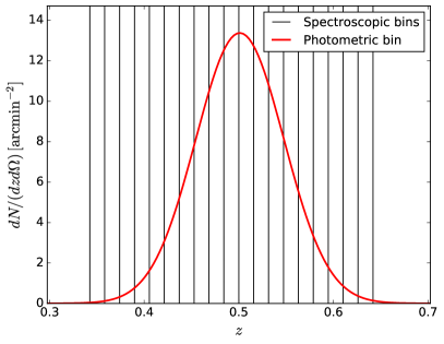
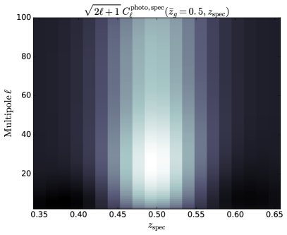
Figure 1: Left panel: example of a redshift bin for a photometric survey and the redshift bins chosen for an overlapping spectroscopic survey. Right panel: amplitude of the cross-correlation with an overlapping spectroscopic survey as a function of spectroscopic redshift bin ($x$ axis) and angular scale ($y$ axis). The amplitude of the cross-correlation traces the redshift distribution, and can therefore be used to constrain it.

II Formalism

II.1 Clustering-based photo-$z$ calibration

Consider two galaxy samples with redshift distributions $\phi_{i}(z)$ ($i=\{1,2\}$), and let $a^{i}_{\ell m}$ be the harmonic coefficients of their projected overdensity of counts on the sky. Their cross-correlation is given by:

$$\langle a^{i}_{\ell m}a^{j*}_{\ell m}\rangle=N^{ij}_{\ell}+S^{ij}_{\ell}$$ (1)

$$S^{ij}_{\ell}=\frac{2}{\pi}\int dz\int dz^{\prime}\,\phi_{i}(z)\phi_{j}(z^{\prime})\times$$ (2)

$$\times\int dk\,k^{2}\,b_{i}(z)b_{j}(z^{\prime})P_{m}(k,z,z^{\prime})\,j_{\ell}(k\chi(z))\,j_{\ell}(k\chi(z^{\prime})),$$

where $P_{m}$ is the matter power spectrum, $\chi$ is the radial comoving distance, $j_{\ell}(x)$ is a spherical Bessel function, $N^{ij}_{\ell}$ is the cross-noise power spectrum between samples $i$ and $j$, $b_{i}$ is the linear bias of the $i$-th sample and we have neglected redshift-space distortions and all other sub-dominant contributions to the observed power spectrum. In the Limber approximation - where $j_{\ell}(x)\rightarrow\sqrt{\pi/(2\ell+1)}\delta^{\mathcal{D}}(\ell+1/2-x)$ - this expression simplifies to:

$$S^{ij}_{\ell}=\int dk\,P_{m}(k,z_{\ell})\,\frac{H^{2}(z_{\ell})b^{i}(z_{\ell})b^{j}(z_{\ell})}{\ell+1/2}\phi_{i}(z_{\ell})\phi_{j}(z_{\ell}),$$ (3)

where $\chi(z_{\ell})\equiv(\ell+1/2)/k$.

For the purposes of this discussion, the most important feature of Equation 3 is the fact that the amplitude of the cross-correlation is proportional to the overlap between the redshift distributions of those samples. This is especially relevant if one of the samples has good radial resolution, in which case it can be split into narrow bins of redshift. The cross-correlations of all narrow bins with the other sample will therefore trace the amplitude of its redshift distribution, and can effectively be used to constrain it. This is illustrated in Fig. 1, which shows the cross-power spectrum between a Gaussian photo-$z$ bin of width $\sigma=0.05$ and a set of narrow redshift bins ($\delta z\sim 0.002$).

Note also that Eq. 3 implies that the redshift distribution and the redshift-dependent galaxy bias of the photometric sample are completely degenerate in this method, and therefore additional information is needed in order to separate both quantities (e.g. including prior information or lensing data). Since this is an inherent problem of the method, and not specific to the case of intensity mapping, we will simply assume that $b(z)$ is a sufficiently smoothly-varying function of $z$, thus treating IM and spectroscopic surveys on an equal footing. The more complicated biasing scheme that arises on small scales also prevents the use of those modes to constrain $\phi(z)$ Schmidt et al. (2013), and therefore one must be conservative when deciding the range of scales to include in the analysis.

Different recipes have been formulated to carry out this kind of analysis, such as the optimal quadratic estimator method of McQuinn and White (2013). The forecasts presented here will interpret the redshift distribution (in a parametric or non-parametric form) as a set of extra nuisance parameters, on which we will carry out the Fisher matrix analysis described in Section II.5. Thus, even though our results will be optimistic in as much as the Fisher matrix saturates the Rao-Cramer bound, they will account for all correlations between redshift distribution parameters and with the cosmological parameters, as well as the presence of redshift-space distortions and magnification bias (effects that have been overseen in previous works).

For the purposes of estimating the ability of future surveys to calibrate photometric redshift distributions through cross-correlations, we will always consider an individual redshift bin for a photometric sample with unknown distribution, together with a set of overlapping narrow redshift bins of spectroscopic galaxies or intensity mapping observations. Let $N^{p}(z)$ be the overall true redshift distribution of the photometric sample, and let $p(z_{\rm ph}|z)$ be the conditional distribution for a photo-$z$ $z_{\rm ph}$ given the true redshift $z$. Then, the redshift distribution in a photo-$z$ redshift bin $b$ with bounds $z_{b}^{i}<z_{\rm ph}<z_{b}^{f}$ is given by

$$\phi_{b}(z)\propto N^{p}(z)\int_{z_{b}^{i}}^{z_{b}^{f}}dz_{\rm ph}\,p(z_{\rm ph}|z).$$ (4)

In what follows we will consider two degrees of complexity in terms of describing the unknown redshift distribution:

1. We will assume Gaussian photo-$z$s with a given variance ($\sigma_{z}^{2}$) and bias $\Delta z$:

   $$p(z_{\rm ph}|z) \equiv\mathcal{N}(z_{\rm ph}-\Delta z;z,\sigma_{z})$$

   $$\equiv\frac{\exp\left[-\frac{1}{2}\frac{(z_{\rm ph}-z-\Delta z)^{2}}{\sigma_{z}^{2}}\right]}{\sqrt{2\pi\sigma_{z}}},$$ (5)

   and we will assume that the uncertainty in the redshift distribution is fully described by $\Delta z$ and $\sigma_{z}$.

2. We will use a non-parametric form for $\phi_{b}(z)$, given as a piecewise function with a free amplitude for each spectroscopic redshift bin.

Our assumed fiducial value for $\Delta z$ and $\sigma_{z}$, as well as the binning scheme used are described in Section II.2.

We finish this section by noting that the use of cross-correlations with spectroscopic surveys or intensity mapping observations for photo-$z$ calibration is not limited to the measurement of the redshift distribution of a given galaxy sample, but that they can also be used to improve the precision of photometric redshift estimates for individual galaxies (e.g. Jasche and Wandelt (2012)). Although we leave the discussion of this possibility for future work, we describe a Bayesian formalism for this task in Appendix A.

II.2 Photometric redshift surveys

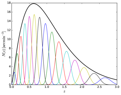
Figure 2: Angular number density of galaxies as a function of redshift for the LSST gold sample (solid black line). The colored lines show the window functions of the 15 redshift bins considered here.

This section describes the model used here for a LSST-like photometric redshift survey. As in Alonso and Ferreira (2015), we base our description of the number density of sources and their magnification bias on the measurements of the luminosity function of Gabasch et al. (2006), with $k$-corrections computed with kcorrect Blanton and Roweis (2007). We assume a magnitude cut of $25.3$ in the $i$ band, corresponding to the so-called “gold” sample LSST Collaboration et al. (2009). Unlike Alonso and Ferreira (2015), and for simplicity, we will consider a single galaxy population, instead of splitting it into “red” and “blue” sources. The resulting redshift distribution is shown by the solid black line in Figure 2.

We model the linear galaxy bias as a function of redshift as $b(z)=1+0.84z$, based on the simulations of Weinberg et al. (2004), and quoted in the LSST science book LSST Collaboration et al. (2009).

The photometric redshift requirement for the gold sample as stated in the LSST science book are $\sigma_{z}/(1+z)<0.05$, with a goal of $0.02$. Here we have taken a conservative estimate, assuming a standard deviation $\sigma_{z}=0.03(1+z)$. We then split the full sample into redshift bins with a width given by $3\times\bar{\sigma}_{z}$, where $\bar{\sigma}_{z}$ is the photo-$z$ variance at the bin centre. This binning scheme is chosen to reduce the correlation between bins induced by the tails of the photo-$z$ distribution, and results in the 15 redshift bins shown in Fig. 2 (where the redshift distributions are computed with Eq. 4). Our fiducial photo-$z$ model will assume biased Gaussian distributions, fully determined by $\sigma_{z}$ and $\Delta z$.

II.3 Intensity mapping

Experiment	SKA	MeeKAT	HIRAX
$T_{\rm inst}$	25K	25 K	50 K
$t_{\rm tot}$	10000 h	4000 h	$2.8\times 10^{4}$ h
$N_{\rm dish}$	197	64	1024 ($32\times 32$)
$D_{\rm dish}$	15 m	13.5 m	6 m
$\nu$ range	350-1050 MHz	600-1050 MHz	400-800 MHz
$f_{\rm sky}$	0.4	0.1	0.4

Table 1: Experimental specifications assumed for SKA, MeerKAT and HIRAX. The baseline distributions for each experiment are described in Section II.3. Note that the frequency ranges above correspond to the UHF band of SKA and MeerKAT.

Intensity mapping (IM) is a novel observational technique that circumvents the long integration times needed to obtain reliable spectroscopic redshifts for individual objects through an approach that is transverse to that used by photometric surveys. The idea (McQuinn et al., 2006; Wyithe and Loeb, 2008; Peterson et al., 2009; Switzer et al., 2013) is to observe the unresolved combined emission of many line-emitting sources in a relatively wide pixel at different frequencies. The signal-to-noise ratio of the corresponding line emission is much stronger than that of the individual sources, and thus, combining the intensity measured across the sky and relating the intensity observed at a given frequency to the rest-frame wavelength of the emission line it is possible to produce three-dimensional maps of the density of the line-emitting species. This technique is particularly appealing for isolated spectral lines, as is the case of the 21cm line caused by the spin-flip transition in neutral hydrogen atoms (HI), and thus HI intensity mapping has been proposed as an ideal method to cover vast volumes at relatively low cost.

A number of experiments have been proposed to carry out IM measurements of the baryon acoustic oscillation scale, such as BINGO Battye et al. (2012), CHIME Newburgh et al. (2014), FAST Bigot-Sazy et al. (2016), HIRAX Newburgh et al. (2016), SKA Santos et al. (2015) and Tianlai Chen (2011). The different instrumental approaches to IM can be broadly classified into two camps:

• Interferometers: the sky emission is measured by a set of antennas, and the measurements of pairs of antennas separated by a given baseline ${\bf d}$ are cross-correlated to produce the measurement of an angular Fourier mode with scale ${\bf l}\sim 2\pi{\bf d}/\lambda$ (where $\lambda$ is the observed wavelength). The intensity map is then reconstructed by combining pairs with different baselines.

• Single-dish: in this case the sky emission is measured and auto-correlated by individual antennas. A band-limited intensity map with a resolution $\delta\theta\sim\lambda/D_{\rm dish}$ is then produced by varying the antenna pointing, where $D_{\rm dish}$ is the antenna diameter.

The expressions for the noise power spectrum for both cases are derived in Appendix C, and can be summarized as:

$$N^{\nu}_{\bf l}=\frac{T_{\rm sys}^{2}4\pi f_{\rm sky}}{\eta^{2}\Delta\nu t_{\rm tot}}\left\{\begin{array}[]{ll}\frac{1}{N_{\rm dish}B^{2}({\bf l})},&\text{single dish}\\ \frac{\Omega_{p}}{N_{d}({\bf d}={\bf l}\lambda/(2\pi))\lambda^{2}},&\text{interferometer}.\end{array}\right.$$ (6)

Here $T_{\rm sys}$ is the system temperature, given as a combination of instrumental and sky temperature (see Appendix C), $f_{\rm sky}$ is the sky fraction covered by the observations, $\eta^{2}$ is the antenna efficiency, $\Delta\nu$ is the bandwidth in that channel, $t_{\rm tot}$ is the total observation time for the survey, $N_{\rm dish}$ is the number of dishes, $B({\bf l})$ is the harmonic transform of the antenna beam, $N_{d}({\bf d})$ is the distribution of baselines and $\Omega_{p}$ is the solid angle covered per pointing. For all experiments discussed here we will assume $\eta=1$, Gaussian beams so that $B({\bf l})=\exp[-\ell(\ell+1)\theta_{\rm FWHM}^{2}/(16\log 2)]$, and $\Omega_{p}=\theta_{\rm FWHM}^{2}$, where $\theta_{\rm FWHM}$ is the beam full-width at half maximum, which will approximate as $\theta_{\rm FWHM}=1.22\lambda/D_{\rm dish}$. Note that the baseline distribution $N_{d}$ is normalized such that:

$$\frac{N_{\rm dish}(N_{\rm dish}-1)}{2}=\int d{\bf d}^{2}\,N_{d}({\bf d}),$$ (7)

where $N_{\rm dish}(N_{\rm dish}-1)/2$ is the total number of independent baselines.

Given their expected full overlap with LSST, we will consider here the two main currently envisaged southern-hemisphere intensity mapping experiments: SKA (and its pathfinder, MeerKAT) and HIRAX.

II.3.1 MeerKAT and the SKA

MeerKAT is the 64-dish precursor to the mid-frequency component of the SKA. MeerKAT is comprised of 13.5 metre dishes and will operate between $\sim 550-3$ GHz using three separate receivers. Although, it will predominantly used as an interferometer, and as such only be sensitive to relatively small spatial scales, there is a proposed project to use MeerKAT in single-dish mode Fonseca et al. (2017). If such a mode of operation is viable, then MeerKAT will become an extremely efficient intensity-mapping facility operating at frequencies that allows the detection of Hi to $z\sim 1.5$. Indeed, a proposed open-time survey would provide a several thousand square degree sky survey over the Dark Energy Survey and/or Kilo-degree Survey areas, which will provide excellent visible wavelength coverage.

In the 2020s, MeerKAT will be enhanced by the addition of 130, 15 metre dishes to form the mid-frequency SKA. Operating at similar frequencies to MeerKAT, the additional 130 dishes will provide much more sensitivity for all science aims, and is capable of carrying out a $\sim 10,000$ deg² intensity mapping survey Santos et al. (2015).

As such, both MeerKAT and the SKA will provide a unique view on the Hi Universe, and as we will show, can enhance the cosmological science with the LSST with cross-correlations.

II.3.2 HIRAX

The Hydrogen Intensity mapping and Real-time Analysis eXperiment (HIRAX) is a proposed close-packed radio array comprising 1024 six metre dishes disposed in a $32\times 32$ grid and operating at 400-800 MHz. The telescope will be located on the South African Karoo site, which has very low levels of RFI in this band, and provides an ideal location to overlap in sky coverage with other planned southern sky cosmological surveys. The large collecting area and field-of-view provide excellent sensitivity and mapping speed, with the high density of short baselines allowing for sensitive measurements of the baryon acoustic oscillation (BAO) scale in the cosmic HI distribution from redshift $\sim$0.8 to 2.5, which in turn will provide competitive constraints on dark energy (Newburgh et al., 2016). HIRAX will make high signal-to-noise maps of 21cm intensity fluctuations over 15,000 sq degrees (taken to overlap fully with LSST) on cosmological scales of interest, with the relatively high frequency resolution (1024 channels over the 400 MHz bandwidth) allowing for accurate redshift calibration of 21cm intensity maps. This makes it ideal for calibration of LSST photometric redshifts through the cross-correlation technique.

II.3.3 Generic IM experiment

Besides SKA and HIRAX we will also explore the capabilities of a generic intensity mapping experiment in terms of photo-$z$ calibration. The performance of a given experiment is roughly determined by three quantities:

• The range of angular scales over which the noise power spectrum is low enough to probe the cosmological HI emission. This range can be characterized by the minimum and maximum baselines $d_{\rm min}$ and $d_{\rm max}$.

• The noise level (normalized by the bandwidth $\Delta\nu$) $\sigma_{T}$ on this range of scales. For a fixed integration time, this is determined by the system temperature $T_{\rm sys}$ and the observed sky area $f_{\rm sky}$.

Here we will model the effects of the minimum and maximum baselines as a sharp and an inverse-Gaussian cutoff respectively. Thus, our model for the angular noise power spectrum is:

$$N^{\nu}_{\ell}=\frac{\sigma^{2}_{T}}{\Delta\nu}\left[\Theta\left(\frac{\ell\lambda}{2\pi},d_{\rm min}\right)\right]^{-1}\exp\left[\ell(\ell+1)\frac{\theta_{\rm beam}^{2}}{8\log 2}\right],$$ (8)

where $\theta_{\rm beam}\equiv 1.22\lambda/d_{\rm max}$ and $\Theta(x,x_{i})$ is 1 if $x_{i}<x$ and 0 otherwise. Note that by definition $\sigma_{T}$ has units of $[{\rm mK}\,{\rm rad}\,{\rm MHz}^{1/2}]$. For comparison, the equivalent values of these parameters that roughly reproduce the noise curves for HIRAX are:

$$d^{\rm HIRAX}_{\rm min}=6\,{\rm m},\hskip 12.0ptd^{\rm HIRAX}_{\rm max}\sim 300\,{\rm m},$$

$$\sigma^{\rm HIRAX}_{T}\sim 10^{-3}\,{\rm mK}\,{\rm rad}\,{\rm MHz}^{1/2}$$

II.3.4 Foregrounds

One of the main obstacles that HI intensity mapping must overcome to become a useful cosmological tool is the presence of galactic and extragalactic foregrounds several orders of magnitude larger than the 21cm cosmological signal Santos et al. (2005); Wolz et al. (2014). Under the assumption that foregrounds are coherent in frequency (as opposed to the cosmic signal tracing the density inhomogeneities along the line of sight), these foreground sources can be in principle efficiently removed using component-separation methods Wolz et al. (2014); Shaw et al. (2015); Alonso et al. (2015). However, instrumental imperfections, such as frequency-dependent beams or polarisation leakage, can generate foreground residuals with a non-trivial frequency structure that could strongly bias cosmological constraints from 21cm data alone. In any case, the removal of frequency-smooth components will introduce large uncertainties on the large-scale radial modes of the 21cm fluctuations.

Here we have introduced the effect of foregrounds by including an extra component, $f$, in the sky model for HI accounting for foreground residuals. Thus we will assume that the measured harmonic coefficients at a given frequency $\nu$ are given by:

$$a^{\nu}_{\ell m}=s^{\nu}_{\ell m}+f^{\nu}_{\ell m}+n^{\nu}_{\ell m},$$ (9)

where $s^{\nu}_{\ell m}$ and $n_{\ell m}$ are the true cosmological signal and the instrumental noise contribution. We will model $f$ as an almost-correlated component with a cross-frequency power spectrum given by

$$C^{\nu\nu^{\prime}}_{f,\ell m} \equiv\langle f^{\nu}_{\ell m}f^{\nu^{\prime}*}_{\ell m}\rangle$$

$$=A_{\rm FG}\left(\frac{\ell}{\ell_{*}}\right)^{\beta}\left(\frac{\nu\nu^{\prime}}{\nu_{*}^{2}}\right)^{\alpha}\exp\left[-\frac{{\rm log}^{2}(\nu/\nu^{\prime})}{2\xi^{2}}\right].$$ (10)

Here $A_{\rm FG}$ and $\beta$ parametrise the amplitude of the foreground residuals and their distribution on different angular scales, and $\alpha$ describes their mean frequency dependence. Finally, $\xi$ parametrises the characteristic frequency scale over which foregrounds are decorrelated. When including the effects of foregrounds (Section III.3) we will also marginalize over $(A_{\rm FG},\alpha,\beta,\xi)$. For $\alpha$ and $\beta$ we will use the fiducial values $\alpha=-2.7$ and $\beta=-2.4$, corresponding to galactic synchrotron emission Santos et al. (2005); Planck Collaboration et al. (2016), and we will set $A_{\rm FG}=1\,{\rm mK}^{2}$, large enough for the residuals to dominate the equal-$\nu$ power spectrum. We will study the final constraints as a function of $\xi$.

Effectively, this extra component cancels the constraining power of all radial modes of the 21cm fluctuations with comoving radial wavenumbers $k_{\parallel}$ below a scale $k_{\parallel}^{\rm FG}$, related to $\xi$ through

$$k_{\parallel}^{\rm FG}\sim\frac{\pi\,H(z)}{c\,(1+z)\,\xi}$$ (11)

The effect of foregrounds on the ability to constrain redshift distributions can be readily understood as loss of information in the $k_{\parallel}-k_{\perp}$ space. In the flat-sky approximation, and on linear scales, the angular power spectrum between two tracers $i$ and $j$ of the matter density can be computed as:

$$C^{ij}_{k_{\perp}}=\int\frac{dk_{\parallel}}{2\pi}P(k_{\parallel},k_{\perp})W^{i}(k_{\parallel})W^{j*}(k_{\parallel}),$$ (12)

where we have again ignored the effect of redshift-space distortions and:

$$W^{k}(k_{\parallel})\equiv\int dx_{\parallel}\,\phi^{k}(x_{\parallel})b^{k}(x_{\parallel})D(x_{\parallel})e^{ix_{\parallel}k_{\parallel}}.$$ (13)

Here $D$ is the linear growth factor and $b^{k}$ and $\phi^{k}$ are the linear bias and selection function for the $k$-th tracer. Let us assume that $i$ is a photometric redshift bin and $j$ is a narrow intensity mapping frequency shell with comoving width $\delta\chi$ centered at $\chi_{*}$. Assuming $D$ and the bias $b^{j}$ to be slowly-varying functions of $\chi$ we obtain:

$$C^{ij}_{k_{\perp}}=\int\frac{dk_{\parallel}}{2\pi}P(k_{\parallel},k_{\perp})W^{i}(k_{\parallel})D(\chi_{*})b^{j}(\chi_{*})j_{0}(k_{\parallel}\delta\chi/2).$$ (14)

Now, assuming that $\phi^{i}$ has support over a wide range of redshifts, corresponding to a comoving width $\Delta\chi$, its Fourier transform ($\sim W^{i}$) will only have support over wavenumbers $k_{\parallel}\lesssim 1/\Delta\chi$. Since the Bessel function $j_{0}$ provides support over all values of $k_{\parallel}\lesssim 1/\delta\chi$, and under the assumption that $\delta\chi<\Delta\chi$, the total number of modes that contribute to $C^{ij}$ is bound by $\sim 1/\Delta\chi$. Since foreground contamination will mostly affect large radial modes, eventually a large fraction of this $k_{\parallel}$-range becomes dominated by foreground uncertainties and stops contributing efficiently to the overall signal-to-noise ratio, thus degrading the final constraints on any model parameter.

We finish this Section by noting that, as described in Section II.1, the main constraining power for photo-$z$ calibration comes from the cross-correlation of the photometric and spectroscopic samples. Since the photometric sample would not suffer from foreground contamination, these cross-correlations are very robust against foreground biasing, which makes photo-$z$ calibration an ideal application of IM.

II.4 Spectroscopic surveys

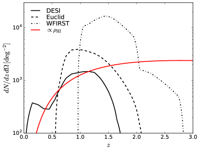
Figure 3: Angular number density of galaxies as a function of redshift for the three spectroscopic surveys considered here: DESI (solid), Euclid (dashed) and WFIRST (dot-dashed). The red solid line shows the redshift dependence of the mean HI density (arbitrarily normalized) for comparison.

In order to showcase the possibility of calibrating redshift distributions through cross-correlation with future intensity mapping experiments we will compare their forecast performance against that of the most relevant future spectroscopic suveys:

• The Dark Energy Spectroscopic Instrument (DESI) Levi et al. (2013) is a spectroscopic galaxy survey planned to cover $\sim 14000\,{\rm deg}^{2}$ from its northern-hemisphere location at Kitt Peak National Observatory. We assume an area overlap of $f_{\rm sky}=0.2$ with LSST, and we model the number density and clustering bias of the two galaxy samples considered here (Luminous Red Galaxies and Emission Line Galaxies) as done in Font-Ribera et al. (2014).

• The Euclid galaxy survey Laureijs et al. (2011) is a space-borne infrared spectrograph that will aim to detect $\sim 5\times 10^{7}$ H$\alpha$-emitting galaxies in the redshift range $0.65<z<2$ over $\sim 15000\,{\rm deg}^{2}$. We assume full overlap with LSST, and we model the number density and bias as in Font-Ribera et al. (2014).

• The Wide Field Infrared Survey Telescope (WFIRST) Spergel et al. (2013) is a future space observatory in the infrared that will measure redshifts for $\sim 2.6\times 10^{7}$ objects over $\sim 2000\,{\rm deg}^{2}$. The deep nature of WFIRST will make it ideal to calibrate the LSST redshift distribution at high redshifts. We model the number density and bias of the WFIRST sample as in Font-Ribera et al. (2014), and we assume a full overlap with LSST ($f_{\rm sky}=0.05$).

Figure 3 shows the redshift distributions for galaxies detected by these three experiments.

II.5 Forecasting formalism

Our formalism will distinguish between two types of tracers of the density field:

• Spectroscopic: tracers whose redshift distribution is well known. This would correspond to tracers with good radial resolution such as a narrow redshift bin of spectroscopic sources or an intensity map in a narrow frequency band, as well as other tracers with a well-known window function, such as a CMB lensing map.

• Photometric: tracers whose redshift distribution is unknown or uncertain. This would correspond to e.g. a photometric-redshift bin, a radio continuum survey or a map of the Cosmic Infrared Background.

Let us start by considering a set of sky maps corresponding to a number of tracers, and let ${\sf a}$ be the corresponding vector of maps expressed in a given basis. In the following sections we will assume that ${\sf a}$ is stored in terms of spherical harmonic coefficients and that it takes the form ${\sf a}_{\ell m}=(p_{\ell m},s^{1}_{\ell m},...s^{N_{s}}_{\ell m})$, where $p_{\ell m}$ is a photometric tracer and $s^{i}_{\ell m}$ is a set of spectroscopic tracers. For the moment, however, we will keep the discussion general.

Assuming that ${\sf a}$ is Gaussianly distributed with zero mean and covariance $\hat{\sf C}\equiv\langle{\sf a}{\sf a}^{\dagger}\rangle$, its log-likelihood is given by:

$$\mathcal{L}\equiv-2\log p({\sf a})={\sf a}^{\dagger}\hat{\sf C}^{-1}{\sf a}+\log(\det(2\pi\hat{\sf C})).$$ (15)

Now let $q_{i}$ be a set of parameters modelling $\hat{\sf C}$, including (but not limited to) the parameters describing the photometric redshift distribution. A maximum-likelihood estimator for $q_{i}$ can be defined by using an iterative Newton-Raphson method to minimize Eq. 15. This is described in Tegmark et al. (1998); Bond et al. (1998); McQuinn and White (2013), and yields the iterative algorithm:

$$q_{i}^{n}=q_{i}^{n-1}+[\hat{\sf F}^{-1}]_{ij}\left[{\sf a}^{\dagger}\hat{\sf C}^{-1}\hat{\sf C}_{,j}\hat{\sf C}^{-1}{\sf a}-{\rm Tr}(\hat{\sf C}_{,j}\hat{\sf C}^{-1})\right],$$ (16)

$$\hat{\sf F}_{ij}\equiv\left\langle\frac{\partial^{2}\mathcal{L}}{\partial q_{i}\partial q_{j}}\right\rangle={\rm Tr}\left(\hat{\sf C}^{-1}\hat{\sf C}_{,i}\hat{\sf C}^{-1}\hat{\sf C}_{,j}\right),$$

where, in Eq. 16 there is an implicit summation over $j$, the sub-index _,i implies differentiation with respect to $q_{i}$, $\hat{\sf F}$ is the Fisher matrix, $q_{i}^{n}$ is the $n-$th iteration of the solution for $q_{i}$ and the previous iteration $q_{i}^{n-1}$ is used to compute $\hat{\sf C}$ and $\hat{\sf C}_{,i}$ in the second term. Note that we have simplified a pure Newton-Raphson iteration by taking the ensemble average of the likelihood Hessian (i.e. the Fisher matrix). Furthermore, in the case where the likelihood is well-approximated by a Gaussian, $\hat{\sf F}^{-1}$ is the covariance matrix of the $q_{i}$. Eq. 16 is the basis of the method proposed in McQuinn and White (2013) (with a number of simplifications) and used in Johnson et al. (2017) to constrain the redshift distribution of galaxies in the KiDS survey.

In our case, we mainly care about the uncertainty in the redshift distribution parameters included in the $q_{i}$, and therefore we will simply estimate the Fisher matrix $\hat{\sf F}$. In the case where ${\sf a}$ is a set of spherical harmonic coefficients with power spectrum $\langle{\sf a}_{\ell m}{\sf a}^{\dagger}_{\ell^{\prime}m^{\prime}}\rangle=\delta_{\ell\ell^{\prime}}\delta_{mm^{\prime}}\hat{\sf C}_{\ell}$, $\hat{\sf F}$ is given by

$$\hat{\sf F}_{ij}=\sum_{\ell=2}^{\ell_{\rm max}}f_{\rm sky}(\ell+1/2)\,{\rm Tr}\left(\hat{\sf C}^{-1}_{\ell}\hat{\sf C}_{\ell,i}\hat{\sf C}^{-1}_{\ell}\hat{\sf C}_{\ell,j}\right),$$ (17)

where we have approximated the effects of a partial sky coverage by scaling the number of independent modes per $\ell$ by the sky fraction $f_{\rm sky}$. The form of the power spectra $\hat{\sf C}_{\ell}$ for the different tracers considered in this work is given in Appendix B.

As explicitly shown in Eq. 17, smaller-scale modes carry a higher statistical weight (proportional to $\sim\ell$), and would in principle dominate the redshift distribution constraints. The smallest scales are, however, dominated by theoretical uncertainties from non-linearities in the evolution of the density field and the galaxy-halo connection, and therefore a multipole cutoff $\ell_{\rm max}$ must be used to contain the constraining power of systematics-dominated modes. In this paper we use a redshift-dependent cutoff defined as follows. Let $z$ be the mean redshift of a given redshift bin, and let $\sigma^{2}(k_{*})$ be the variance of the linear density field at that redshift on modes with wavenumber $k<k_{*}$:

$$\sigma^{2}(k_{*},z)\equiv\frac{1}{2\pi^{2}}\int_{0}^{k_{*}}dk\,k^{2}\,P_{m}(k,z).$$ (18)

We then define the cutoff scale as $\ell_{\rm max}(z)=\chi(z)\,k_{\rm max}(z)$, where $k_{\rm max}(z)$ satisfies $\sigma(k_{\rm max},z)=\sigma_{\rm thr}$ for some choice of $\sigma_{\rm thr}$. In what follows we will use a fiducial threshold $\sigma_{\rm thr}=1$, corresponding to $k_{\rm max}(z=0)\simeq 0.3\,h\,{\rm Mpc}^{-1}$, and we will study the dependence of our results on this choice. Besides this choice of $\ell_{\rm max}$, we will also impose a hard cutoff for all galaxy-survey and intensity-mapping tracers of $\ell<2000$ (thus, in reality, $\ell_{\rm max}={\rm min}(\chi k_{\rm max},2000)$).

III Results

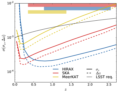
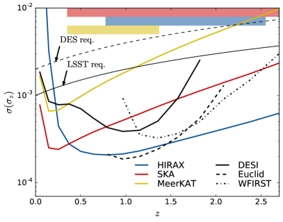
Figure 4: Left panel: forecast 1$\sigma$ constraints on the photo-$z$ scatter $\sigma_{z}$ (solid lines) and bias $\Delta z$ (dashed lines) for the three IM experiments under consideration: HIRAX (blue), SKA (red) and MeerKAT (yellow). Right panel: comparison of the previous three intensity mapping experiments, in terms of the forecast constraints on $\sigma_{z}$, with three future spectroscopic surveys: DESI (black solid), Euclid (black dashed) and WFIRST (black dot-dashed). In both panels, the thin solid line shows the photo-$z$ calibration requirement on both $\sigma_{z}$ and $\Delta z$ for LSST, with the corresponding requirement for DES shown as a thin dashed line in the right panel. The coloured bands in the upper part of all plots show the proposed frequency ranges for the three 21cm experiments (same color code). We have assumed using the UHF band for SKA and MeerKAT. The L-band would be able to cover all redshifts below $z\sim 0.35$.

In order to forecast for the ability of future experiments to constrain photometric redshift distributions, in the following sections we will use the formalism described in Section II.5 with a data vector given by ${\sf a}_{\ell m}=(p_{\ell m},s^{1}_{\ell m},...,s^{N_{s}}_{\ell m})$, where $p$ is a photometric redshift bin and $s^{i}$ are a set of overlapping redshift bins for a spectroscopic tracer (either an intensity mapping experiment or a spectroscopic galaxy survey). The number $N_{s}$, width and redshift range of the spectroscopic redshift bins is chosen in order to adequately sample the changes in the photometric redshift distribution. We choose the redshift bin width to be $33\%$ of the photo-$z$ uncertainty $\sigma_{z}$, which governs the variability of the redshift distribution (i.e. each redshift interval of $\sigma_{z}$ is sampled in 3 points). In order to sample the tails of the distribution we then define the redshift range of the set of spectroscopic bins as $[z_{b}^{i}-3\sigma_{z},z_{b}^{f}+3\sigma_{z}]$, where $z_{b}^{i}$ and $z_{b}^{f}$ are the edges of the photometric redshift bin. The number of spectroscopic redshift bins $N_{s}$ is then defined in terms of these numbers.

The model parameters $q_{i}$ in the following sections will be given by:

• All of the parameters needed to determine the redshift distribution ($\sigma_{z}$, $\Delta z$ or the amplitude $N(z)$ in different spectroscopic bins, depending on the case).

• Two overall clustering bias parameters, $b_{\rm p}$ and $b_{\rm s}$, corresponding to the bias of the photometric and spectroscopic tracers.

• We will also include two cosmological parameters: the fractional matter density $\Omega_{M}$ and the amplitude of scalar perturbations $A_{\rm s}$, in $q_{i}$ in order to account for the possible cosmology dependence of the results.

We will change this setup in Section III.5, where we will explore the impact of the achieved constraints on the photo-$z$ parameters on the final cosmological constraints. In this section ${\sf a}$ will correspond to the 15 photometric redshift bins for LSST, for both galaxy clustering and weak lensing (i.e. 30 sets of spherical harmonics). Likewise $q_{i}$ will contain the cosmological parameters $(\omega_{c},\omega_{b},h,w_{0},w_{a},A_{s},n_{s},\tau_{\rm reio})$ as well as all the baseline photo-$z$ parameters ($\Delta z$ and $\sigma_{z}$ for all redshift bins), with priors corresponding to the constraints found in the preceding sections.

III.1 Baseline forecasts

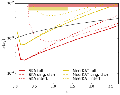
Figure 5: Forecast constraints on the LSST photo-$z$ scatter $\sigma_{z}$ for SKA (red) and MeerKAT (yellow) assuming only interferometric observations (dot-dashed lines), single-dish observations (dashed lines) and both simultaneously (solid lines).

Using the formalism described above, and in the simplified scenario of Gaussian photo-$z$s, we present, in the left panel of Figure 4, the forecast constraints on the photo-$z$ bias ($\Delta z$) and variance ($\sigma_{z}$) for the key intensity mapping experiments introduced in Section II.3. In this and all subsequent plots, the thin black solid line shows the LSST requirement of $\sigma(\Delta z,\sigma_{z})\lesssim 10^{-3}(1+z)$ Newman et al. (2015); de Putter et al. (2014), while the thin dashed line corresponds to the nominal requirement for the Dark Energy Survey ($2\times 10^{-3}$) The Dark Energy Survey Collaboration (2005). The coloured bars in these and all subsequent plots show the redshift ranges corresponding to the proposed frequency bands of the three IM experiments explored here.

Two key features must be noted in this figure: first, the uncertainties grow steeply at low redshifts. This is due to the reduced number of modes available in that regime, associated with the smaller comoving volume and the impact of non-linearities on lower values of $k$. The latter effect is especially severe for HIRAX, given its inability to measure angular modes larger than its beam size. Note, however, that this regime lies outside the proposed frequency ranges for both HIRAX ($0.8\lesssim z\lesssim 2.5$) and SKA ($0.35\lesssim z\lesssim 3$).

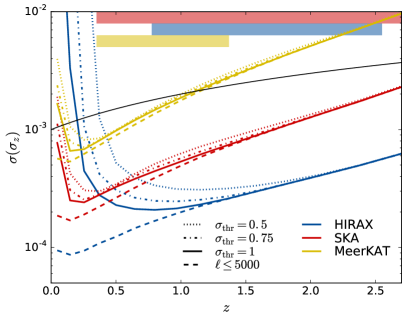
Figure 6: Dependence of the constraints on the LSST photo-$z$ scatter $\sigma_{z}$ on the overdensity variance threshold used to filter out non-linear scales (see Equation 18). The results are shown for HIRAX (blue), SKA (red) and MeerKAT (yellow). The fiducial value used in this analysis is shown as solid lines, while a more optimistic scenario where all multipoles up to $\ell=5000$ are included at all redshifts is shown as a dashed line. This case would mostly benefit interferometric observations, given their higher sensitivity on small angular scales.

Secondly, the ratio between $\sigma(\sigma_{z})$ and $\sigma(\Delta z)$ stays roughly constant ($\sim 1.4$). This is compatible with the expected ratio between the uncertainties associated to the maximum-likelihood estimates of the mean and standard deviation of a Gaussian distribution from a finite number of samples ($\sigma(\sigma)/\sigma(\mu)=\sqrt{2}$). This result holds for most of the cases explored here (see Section III.3 for an exception), and thus we have omitted the curves for $\sigma(\Delta z)$ in most of the subsequent figures.

The right panel of Fig. 4 compares the constraints achievable by IM experiments with those forecast for the spectroscopic surveys described in Section II.4. We see that both SKA and HIRAX would be able to satisfy the LSST requirements over the redshift range of interest. The SKA precursor MeerKAT would fall short except at low redshifts. However, the shorter-term timeline of MeerKAT (2018 onward) would make it an ideal experiment to prove the viability of this technique in cross-correlation with the Dark Energy Survey (DES) The Dark Energy Survey Collaboration (2005), particularly in the light of the proposed intensity mapping surveys Fonseca et al. (2017) targeting a full overlap with DES.

As discussed in Bull et al. (2015), the dish size of SKA is not ideal for cosmological observations, since it is not large/small enough to resolve the angular BAO scale sufficiently well in either single-dish or interferometric modes, although single-dish observations are able to address important science cases such as primordial non-Gaussianity Camera et al. (2013); Alonso and Ferreira (2015). Small scales carry a larger statistical weight, however, and it is not clear that a single-dish strategy would also be ideal for the purposes of photo-$z$ calibration. This is explored in Figure 5, which shows the constraints on $\sigma_{z}$ achievable with single-dish (dashed lines) and interferometric (dash-dotted lines) observations for SKA (red) and MeerKAT (yellow). The constraints from a joint auto- and cross-correlation analysis are shown as solid lines, and correspond to the results reported here. We see that, in the case of SKA, the single-dish mode outperforms the interferometer up to $z\sim 1.4$, when a sufficiently large number of usable modes enter the regime probed by the latter. This suggests that, if simultaneous single-dish and interferometric observations proved to be unfeasible, the photo-$z$ calibration requirements could still be met by using either mode in different redshift ranges.

The performance of this method at low redshift depends crucially on the prescription used to isolate the effect of non-linearities. Here we have done this in terms of the threshold rms variance $\sigma_{\rm thr}$ defined in Eq. 18 for a fiducial value of $\sigma_{\rm thr}=1$, corresponding to $k_{\rm max}\sim 0.3\,{\rm Mpc}^{-1}\,h$ at $z=0$. Figure 6 shows the result of relaxing or tightening this criterion. The effect on SKA and MeerKAT is only moderate, since these experiments gather most of their sensitivity from the large, linear scales in auto-correlation mode. HIRAX, on the other hand, loses sensitivity more rapidly as the scale of non-linearities removes a larger fraction of the available modes. Nevertheless, even for $\sigma_{\rm thr}=0.5$ (corresponding to $k_{\rm max}=0.1\,{\rm Mpc}^{-1}\,h$ at $z=0$) the LSST calibration requirements are satisfied in the redshift range corresponding to the HIRAX frequency band.

III.2 Dependence on experimental parameters

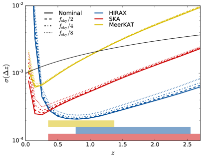
Figure 7: Dependence of the forecast constraints on the LSST photo-$z$ scatter $\sigma_{z}$ on the overlap sky fraction for constant total observation time. In all cases the constraints are mostly insensitive to the trade-off between sky area and noise level, although larger areas are marginally preferred, which reflects the fact that these measurements are mostly dominated by cosmic variance and not noise.

We have so far quantified the potential of currently-proposed experimental configurations for photo-$z$ calibration. The aim of this section is to identify the optimal instrumental specifications for this task.

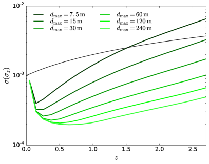
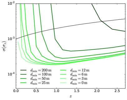
Figure 8: Upper panel: dependence of the forecast constraints on the LSST photo-$z$ scatter $\sigma_{z}$ on the dish size for single-dish IM observations. A dish size of at least $\sim 15{\rm m}$ is needed to match the LSST requirements throughout the whole redshift range. Lower panel: dependence on the minimum baseline for interferometers. Baselines of at most $\sim 12{\rm m}$ are needed to successfully constrain photo-$z$ systematics below $z\sim 0.5$.

We start by exploring the balance between noise level and sky fraction, varying the total overlapping area of the three experiments explored in the previous section (SKA, MeerKAT and HIRAX) keeping the total observation time fixed. The result is presented in Figure 7, which shows the achievable constraints on $\sigma_{z}$ when reducing the sky area by successive factors of 2. We find that, although the results are almost insensitive to the reduction in $f_{\rm sky}$, larger sky areas are always preferred, a reflection of the fact that the constraints are dominated by cosmic variance rather than noise.

As we have discussed in the previous section, the key drawback of single-dish experiments is their inability to access angular scales smaller than the beam size (with their higher statistical weight). Conversely, interferometers are unable to cover scales larger than that probed by their smallest baseline, and therefore they have access to a limited number of reliable (i.e. mildly non-linear) modes. Using the generic instrument parametrization given by Eq. 8, and the fiducial parameters corresponding to HIRAX, Figure 8 explores these issues.

The upper panel shows the constraints achievable by a single-dish experiment for different dish sizes. Dishes of at least 15m (corresponding to the SKA case) are needed in order to achieve the LSST requirements at all redshifts, while a $\sim 100{\rm m}$ dish (e.g. such as the Green Bank Telescope Masui et al. (2013)) would be able to achieve constraints similar to those of HIRAX. The largest currently planned experiment is FAST Bigot-Sazy et al. (2016), with a dish size of 500m.

The lower panel of the figure shows the performance of an interferometer as a function of the minimum baseline $d_{\rm min}$. In this case the main effect is the loss, at lower redshifts, of the large, mildly non-linear scales. A maximum baseline of at most 12m is needed in order to calibrate redshift distributions below $z\sim 0.5$ with sufficient accuracy.

III.3 Foregrounds

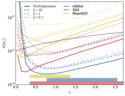
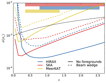
Figure 9: Upper panel: dependence of the forecast constraints on the LSST photo-$z$ scatter on the frequency correlation length of foreground residuals (a measure of the coherence of these residuals across frequencies). Correlation lengths above $\xi\sim 0.1$ (corresponding to radial scales $k_{\parallel}\sim 0.01\,h\,{\rm Mpc}^{-1}$) are necessary to limit the degradation of the photo-$z$ calibration. Lower panel: impact of the foregrounds wedge on the final constraints on the photo-$z$ scatter.

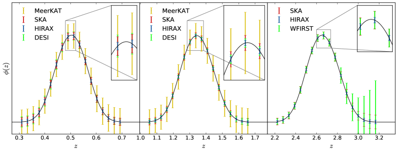
Figure 10: Non-parametric reconstruction of the redshift distribution for four different redshift bins. The points with error bars show the $1\sigma$ constraints on $\phi(z)$ achievable with HIRAX (blue), SKA (red) and MeerKAT (yellow), as well as two spectroscopic surveys (green), DESI and WFIRST, at low and high redshifts respectively. Note that, given the proposed frequency band for HIRAX, it would not be able to calibrate the low and high-redshift bins shown here.

As we discussed in Section II.3.4, the main effect of radio foregrounds for 21cm observations is to make large radial scales (i.e. modes with $k_{\parallel}$ smaller than some $k_{\parallel}^{\rm FG}$) useless. We have parametrised this by introducing an extra component corresponding to foreground residuals characterised by an amplitude $A_{\rm FG}$ and a frequency correlation length $\xi$ (see Section II.3.4 and Eq. 10 for a full description). We set $A_{\rm FG}$ to a value large enough to dominate the emission on radial scales larger than the comoving length corresponding to $\xi$ (see Eq. 11), and study the final constraints as a function of $\xi$.

Figure 9 shows the result of this analysis: while sufficiently coherent foregrounds ($\xi\gtrsim 1$) do not qualitatively modify the final results for the three experiments under consideration, correlation lengths smaller than $\xi\sim 0.1$ would result in a fast degradation of the performance for photo-$z$ calibration. In particular, the associated loss of $k$-space volume would prevent MeerKAT and SKA from reaching the calibration requirements for DES and LSST. The peformance of HIRAX would also be severely compromised by foreground contamination, although it would still be able to reach the required constraints within its proposed frequency range.

These results pose the question of how uncorrelated we can expect foreground residual to be. For reference, raw foreground components are constrained to have correlation lengths of $\xi\sim 1-10$ Santos et al. (2005). On the other hand, more complicated residuals arising from leaked polarised synchrotron would exhibit a much richer frequency structure caused by Faraday rotation, with correlation lengths $\xi\sim 0.1$ at high frequencies ($\sim 800\,{\rm MHz}$) decreasing for longer wavelengths Jelić et al. (2010); Shaw et al. (2015); Alonso et al. (2015). An exquisite instrumental calibration will therefore be necessary in order to optimise the scientific output of 21cm experiments. It is worth noting that the comoving scale corresponding to $\xi\sim 0.1$ ($k_{\parallel}\sim 0.01\,h\,{\rm Mpc}^{-1}$ at $z\sim 1$) is similar to the cut suggested by Shaw et al. (2015), although the expontial form assumed here for the power spectrum of the foreground residuals (Eq. 10) extends the degrading effect into larger wavenumbers.

A further complication comes in the form of the so-called “foreground wedge”, produced by the long time-delay contribution of foregrounds from antennas with far side-lobe responses Datta et al. (2010); Vedantham et al. (2012); Liu et al. (2014); Seo and Hirata (2016). As proven in Parsons et al. (2012); Pober et al. (2014), this effect makes the region of $k$-space defined by:

$$k^{\rm hor}_{\parallel}<\frac{\chi(z)H(z)}{c(1+z)}k_{\perp}$$ (19)

liable to foreground contamination. This is the so-called “horizon” wedge, and corresponds to the case where foreground contamination can be caused by the sources in the horizon picked up by very far sidelobes. Under optimistic assumptions, however, we can consider the case where this effect extends only up to foreground sources located in the outer fringes of the primary beam, in which case the size of the wedge is reduced to the so-called primary-beam wedge Pober et al. (2014), given by $k_{\parallel}^{\rm pb}=\sin(\theta_{\rm FWHM}/2)k^{\rm hor}_{\parallel}$. The lower panel of Figure 9 shows that the LSST photo-$z$ calibration requirements are still met after accounting for the loss of $k$-space to the primary beam wedge.

III.4 Generalized redshift distributions

Even though the simple parametrization of photo-$z$ systematic uncertainties in terms of $\Delta z$ and $\sigma_{z}$ allows us to easily compare the performance of different experiments in terms of photo-$z$ calibration, in a realistic scenario we would like to calibrate generic redshift distributions without assuming a particular parametrization.

This is typically done by promoting the amplitude of the redshift distribution of the photometric sample in each narrow redshift interval to a free parameter that can be constrained from the cross-correlation with the spectroscopic survey. In this section we explore this scenario for the same redshift bins considered in the previous sections.

For this we use the method proposed by McQuinn and White (2013). In essence, this method is equivalent to the formalism outlined in Section II.5, where the free parameters $q_{i}$ considered are the amplitudes of the photometric redshift distribution. The method is further simplified in McQuinn and White (2013) to make it applicable to the analysis of real data using the following approximations:

1. All power spectra are computed using the Limber approximation. This implies (among other things) that all cross-correlations between non-overlapping redshift bins are neglected.

2. The contributions from RSDs and magnification bias are not included in the model for the angular power spectra.

3. No marginalization over cosmological or other nuisance parameters is carried out.

4. The auto-correlation of photometric sources does not contain information about their redshift distribution.

We have adopted these same assumptions here to simplify the discussion.

Figure 10 shows the constraints achievable by different IM experiments and spectroscopic surveys on the generalized form of the redshift distribution for three photometric redshift bins centered around $z\sim 0.5,\,1.35$ and 2.6. The constraining power displayed in this figure matches the results shown in the right panel of Figure 4.

Note that the uncertainties on the amplitude of the redshift distribution found this way can be translated into uncertainties on the two parameters $\Delta z$ and $\sigma_{z}$ used to characterize this distribution in the previous section by performing a simple 2-parameter likelihood analysis for the model in Eqs. 4 and 5. We find that, using this procedure, we recover constraints on $\Delta z$ and $\sigma_{z}$ that are a factor $\sim 2-3$ worse than in the optimal case. This can be understood in terms of the simplifying assumptions adopted here, such as neglecting the information encoded in cross-bin correlations and in the auto-correlation of the photometric sample. In all cases, however, we recover the same relative performance between different experiments in terms of $\sigma(\sigma_{z},\Delta z)$.

III.5 Impact on cosmological constraints

In order to study the impact of photo-$z$ calibration on the final cosmological constraints we have run a Fisher matrix analysis using the formalism described in Section II.5 with the specifications for LSST described in Section II.2. In this case we consider a set of 54 free parameters:

• 3 nuisance parameters for each of the 15 redshift bins: the balaxy bias $b$, the photo-$z$ bias $\Delta z$ and the photo-$z$ scatter $\sigma_{z}$.

• 9 cosmological parameters: the fractional density of cold dark matter $\Omega_{c}\,h^{2}$, the fractional density in baryons $\Omega_{b}\,h^{2}$, the normalized local expansion rate $h$, the amplitude and tilt of primordial scalar perturbations $A_{s}$ and $n_{s}$, the optical depth to reionization $\tau$, the equation of state of dark energy in the $w_{0}$-$w_{a}$ parametrization and the sum of neutrino masses $\sum m_{\nu}$.

In order to pin down the early-universe parameters, we also include information from a hypothetical ground-based Stage-4 CMB experiment Abazajian et al. (2016) using the specifications assumed in Calabrese et al. (2016) and complemented by Planck at low multipoles.

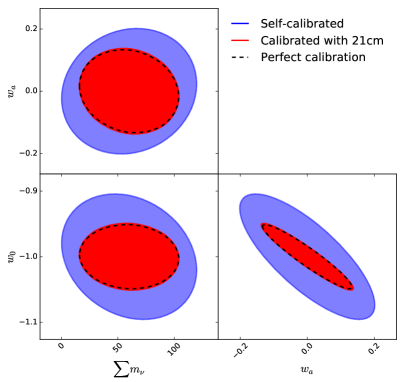
Figure 11: Constraints on the equation of state of dark energy and the sum of neutrino masses in the absence of external photo-$z$ calibration (blue ellipses), with redshift distributions calibrated through cross-correlation with a HIRAX-like 21cm experiment (red ellipses) and in the case of perfect calibration (dashed lines). The constraints also include early-universe information from a Stage-4 CMB experiment.

For the photo-$z$ nuisance parameters we then add Gaussian priors corresponding to the $1\sigma$ uncertainties on $\sigma_{z}$ and $\Delta z$ found using the procedure described in the previous sections for the different experiments considered in this paper. The results of this exercise are displayed in Figure 11, which shows the constraints on the most relevant late-universe parameters: the dark energy equation of state parameters, $w_{0}$ and $w_{a}$, and the sum of neutrino masses. The results shown correspond to the $1\sigma$ contours in the absence of photo-$z$ uncertainties (dashed black line), with photo-$z$ systematics constrained through cross-correlation with a 21cm experiment, in this case HIRAX (red ellipse) and in the absence of external data for photo-$z$ calibration (blue ellipse).

It is important to stress that the overall constraints on these parameters forecast here depend heavily on the survey specifications assumed (e.g. photo-$z$ model and uncertainties), as well as the scales included in the analysis, a point where we have tried to be very conservative. Thus, the results shown in Figure 11 should not be taken to represent the final constraints achievable by LSST. The main result shown in this figure is the relative improvement on the final constraints after photo-$z$ calibration, which should be more robust to these considerations.

Photo-$z$ calibration improves the constraints on each of these parametes by a factor $\sim 1.5-2$, and the dark energy figure of merit by a factor $\gtrsim 5$. Furthermore, we find that the level of calibration achievable through cross-correlations with intensity mapping experiments is nearly equivalent to the case of perfect calibration. Equivalent results are found for SKA and HIRAX, as well as for the combination of DESI, Euclid and WFIRST, as could be expected from the results displayed in the right panel of Figure 4.

IV Discussion

In this paper we have shown that intensity maps of the HI emission can be used to improve the scientific output of photometric redshift surveys. By exploiting the cross-correlations between imaging surveys of galaxies and HI maps, we find that it is possible to optimally calibrate the photometric redshift distributions. This is made clear when assessing improvements in constraints on cosmological parameters: in Figure 11 we see that the FoM using this method is effectively as good as having perfect calibration. This also means that, with the aid of future IM experiments it should be possible to, for example, improve the LSST equation of state figure of merit by approximately a factor of 5.

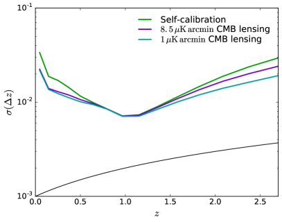
Figure 12: Forecast constraints on the LSST photo-$z$ bias $\Delta z$ in the absence of external datasets (green), and adding CMB lensing data from Stage-3 (purple) and Stage-4 (cyan) CMB experiments.

This approach is promising, but it is important to highlight some of the limitations that have to be overcome if IM is to be used successfully in this context. For a start, it will be important to be able to deal with foreground contamination. In essence, as we have discussed, one can model the effect of foregrounds as a source of noise that cancels the information contained in long-wavelength radial modes. This effect is therefore greatly dependent on how coherent foreground residuals are in frequency. We can expect foregrounds to be highly correlated in intensity, with correlation lengths of order $\xi\sim 1-10$. However, instrumental effects such as polarization leakage or frequency-dependent beams could spoil this coherence and lead to significant losses in the coverage of the $k_{\parallel}$-$k_{\perp}$ plane. We estimate that residuals with correlation lengths $\xi\lesssim 0.1$ (as expected for polarised synchrotron emission, and corresponding to scales $k_{\parallel}\gtrsim 0.01\,h\,{\rm Mpc}^{-1}$ at $z\sim 1$) would significantly degrade the ability of 21cm maps to calibrate redshift distributions efficiently. We have furthermore shown that the calibration requirements of future photometric surveys can also be matched after accounting for the so-called “foregrounds wedge”. Finally, it is worth noting that one of the main strength of the method is its reliance on cross-correlations between the spectroscopic and photometric samples, and that this cross-correlation should be very robust against systematic biases caused by foreground contamination.

If we are to use IM to calibrate future redshift surveys, then we need to make sure that the observational set up satisfies minimum requirements and to do so, we have explored its dependence on experimental parameters. We have found that, for the noise levels of currently proposed experiments, we are primarily limited by cosmic variance and therefore there is no advantage in gaining depth at the cost of sky area: it is preferable to maximize the overlap between the HI maps and the galaxy imaging survey. Furthermore, if we are to accurately capture the longer wave-length modes, we need to resort to single dish observations, a promising but as yet untested mode of observation for MeerKAT and SKA. In the long term, “$1/f$” noise contributions will have to be controlled, and our analysis shows that the dishes must have a minimum size of $\sim 15$ metres. If, on the other hand, we are to use interferometric observations (a method which is more tried and tested) then we need to ensure a minimum baseline of $\sim 12$ metres to capture the large-scale angular modes. We have shown how MeerKAT, HIRAX and SKA fall well within these experimental parameter constraints.

We must also note that our analysis has been conservative in terms of the ranges of scales that add up to the constraints on photo-$z$ parameters, only including angular scales in the regime where non-linear structure formation is believed to be well understood. It may, however, be possible to use even smaller scales for the purposes of photo-$z$ calibration Ménard et al. (2013), in which case some of the conclusions drawn from this analysis could vary. In particular, the relative performance of HIRAX and SKA in terms of photo-$z$ calibration could be significantly different, owing to the higher sensitivity of the SKA interferometer to small angular scales (see Figure 13).

It is interesting to consider alternative approaches to sharpening photometric redshift measurements. Gravitational lensing of the CMB has recently been advocated as a promising approach, given its perfectly well-determined radial kernel (e.g. see Baxter et al. (2016)). We can explore this possibility by considering correlations between LSST and a CMB lensing convergence $\kappa_{\rm CMB}$ map as in Section II.5. We consider two different generations of CMB experiments: an ongoing “Stage-3” experiment, characterised by an rms noise level of $\sigma_{T}\sim 8\,\mu{\rm K}\,{\rm arcmin}$, and a future “Stage-4” experiment with $\sigma_{T}=1\,\mu{\rm K}\,{\rm arcmin}$. In both cases we assume very optimistic configurations, with a beam FWHM of 1 arcmin and using all angular scales $\ell\in[2,3000]$. We also fix all cosmological and bias parameters, and only consider varying $\Delta z$ and $\sigma_{z}$ for each LSST redshift bin. Figure 12 shows the constraint on the photo-$z$ bias $\Delta z$ in the absence of CMB lensing data (green solid line), and using the cross-correlation with $\kappa_{\rm CMB}$ as measured by S3 (purple) and S4 (cyan) experiments. We clearly see that, even under these overly optimistic assumptions, adding CMB lensing information does not significantly help calibrate photo-$z$ uncertainties.

Experiments to undertake intensity mapping of HI are an ongoing effort, and will give us an extremely promising new window on the Universe. We have argued that they will not only contribute in their own right to the further understanding of the large-scale structure of the Universe, but will also help improve the scientific returns from a plethora of up and coming optical surveys.

Appendix A Individual clustering redshifts

The idea of using clustering information to constrain the redshifts of individual objects of a given sample has been considered before in the literature, and shown to yield interesting results even in the absence of spectroscopic data Jasche and Wandelt (2012). Here we outline the steps that should be taken to include intensity mapping information in this formalism.

Our aim is to find the most general expression for the posterior distribution of the true redshifts of a set of galaxies for which we only have photometric data and an overlapping intensity mapping survey. We start by considering a data vector ${\bf d}$ consisting of:

• $\hat{\bf n}$: galaxy positions.

• ${\bf m}$: galaxy magnitudes.

• $\delta_{\rm HI}$: a map of the perturbation in the HI density across angles and redshift

For each galaxy we want to estimate a redshift $z_{i}$, so let ${\bf z}$ be a vector containing all those redshifts. We want to study the posterior probability $p({\bf z}|\delta_{\rm HI},\hat{\bf n},{\bf m})$. Let us start by noting that, in the standard models of large-scale structure, both $\delta_{\rm HI}$ and the galaxy distribution can be thought of as being biased and noisy representations of the underlying matter overdensity $\delta_{\rm M}$. Sampling the galaxy redshifts could then also give us information about $\delta_{\rm M}$, and therefore it’s worth considering the joint distribution $p({\bf z},\delta_{\rm M}|\delta_{\rm HI},\hat{\bf n},{\bf m})$.

One can study this distribution by iteratively sampling the two conditional distributions:

$$\delta_{\rm M}^{i+1}\leftarrow p(\delta_{\rm M}|{\bf z}^{i},\delta_{\rm HI},{\bf m},\hat{\bf n}), \hskip 12.0pt{\bf z}^{i+1}\leftarrow p({\bf z}|\delta_{\rm M}^{i+1},\delta_{\rm HI},{\bf m},\hat{\bf n}).$$

We outline these two steps below.

• Conditional density distribution. We start by noting that, if the true redshifts ${\bf z}$ are known, then the photometric redshifts given by the magnitudes ${\bf m}$ are of no use in constraining the overdensity field, and therefore

  $$p(\delta_{\rm M}|\delta_{\rm HI},{\bf z},\hat{\bf n},{\bf m}) =p(\delta_{\rm M}|\delta_{\rm HI},{\bf z},\hat{\bf n})$$ (21)

  $$=p(\delta_{\rm M}|\delta_{\rm HI},\delta_{\rm g}),$$ (22)

  where $\delta_{\rm g}({\bf z},\hat{\bf n})$ is the galaxy overdensity uniquely defined by the galaxy angular coordinates and redshifts. $p(\delta_{\rm M}|\delta_{\rm HI},\delta_{\rm g})$ can then be decomposed using Bayes’ theorem as:

  $$p(\delta_{\rm M}|\delta_{\rm HI},\delta_{\rm g})\propto p(\delta_{\rm g}|\delta_{\rm M})\,p(\delta_{\rm HI}|\delta_{\rm M})\,p(\delta_{\rm M}),$$ (23)

  where, following the same philosophy as above, we have considered that $p(\delta_{\rm g}|\delta_{\rm M},\delta_{\rm HI})=p(\delta_{\rm g}|\delta_{\rm M})$, since $\delta_{\rm HI}$ is just a noisy and biased realization of $\delta_{\rm M}$. All that remains is then to model the conditional distributions $p(\delta_{\rm g}|\delta_{\rm M})$ and $p(\delta_{\rm HI}|\delta_{\rm M})$, which is by no means a cursory matter, but something that can certainly be accomplished in the regime of validity of structure formation models.

• Conditional redshift distribution. Under the assumptions that galaxies are Poisson-distributed over the (biased) matter overdensity, and that the photometric redshift errors are independent of the environmental density, it is possible to show (e.g. Jasche and Wandelt (2012)) that the galaxy redshifts can be sampled individually with the distribution:

  $$p(z|\delta,\hat{n},m)\propto\left[1+b_{\rm g}(\delta_{\rm M})(z,\hat{n})\right]\,p(z|m),$$ (24)

  where $b_{\rm g}(\delta_{\rm M})(z,\hat{n})$ is the galaxy overdensity along the angular direction of each galaxy, and $p(z|m)$ is the prior photo-$z$ distribution.

Appendix B Angular power spectra

This section describes the theoretical models used for the angular power spectra entering the computation of the Fisher matrix (Eq. 17). The cross-power spectrum between two tracers of the cosmic density field, $a$ and $b$, can be estimated as:

$$C^{ab}_{\ell}=4\pi\int_{0}^{\infty}\frac{dk}{k}{\cal P}_{\Phi}(k)W^{a}_{\ell}(k)W^{b}_{\ell}(k),$$ (25)

where ${\cal P}_{\Phi}(k)$ is the power spectrum of the primordial curvature perturbations and $W^{a}_{\ell}(k)$ is the window function for tracer $a$, containing information about the different contributions to the total anisotropy in that tracer and about its redshift distribution.

In the case of galaxy clustering and intensity mapping, and neglecting contributions from magnification bias and large-scale relativistic effects, $W^{a}$ is given by:

$$W^{a}_{\ell}(k)=\int_{0}^{\infty}dz\,\phi_{a}(z)\left[b_{a}(z)T_{\delta}(k,z)j_{\ell}(k\chi(z))+\frac{1+z}{H(z)}T_{\theta}(k,z)j^{\prime\prime}_{\ell}(k\chi(z))\right],$$ (26)

where $H(z)$ and $\chi(z)$ are the expansion rate and radial comoving distance at redshift $z$ respectively, $\phi_{a}(z)$ is the source redshift distribution, and $T_{\delta}$ and $T_{\theta}$ are the transfer functions of the matter overdensity and velocity divergence fields. Note that, even though we include the effect of non-linearities using the non-linear transfer function for $\delta$ (through the prescription of Takahashi et al. (2012)), we only introduce the effect of redshift-space distortions at the linear level, and only consider a deterministic linear bias $b_{a}(z)$. This is, nevertheless, a more rigorous treatment than has been used in the literature, and the procedure used to mitigate the effect of non-linearities described in Section II.5 should minimize the corresponding impact on the forecasts presented here.

For galaxy shear tracers of weak lensing, the expression for the window function is:

$$W^{a}_{\ell}(k)=-\frac{1}{2}\sqrt{\frac{(\ell+2)!}{(\ell-2)!}}\int_{0}^{\infty}\frac{dz}{H(z)}\int_{z}^{\infty}dz^{\prime}\phi_{a}(z^{\prime})\frac{\chi(z^{\prime})-\chi(z)}{\chi(z^{\prime})\chi(z)}T_{\phi+\psi}(k,z)\,j_{\ell}(k\chi(z)),$$ (27)

where $T_{\phi+\psi}$ is the transfer function for the sum of the two metric potentials in the Newtonian gauge.

The computation of Eq. 25 was carried out using a modified version of the Boltzmann code CLASS Blas et al. (2011); Di Dio et al. (2013).

Appendix C Noise power spectrum for intensity mapping experiments

This section derives the expression for the noise power spectra of single-dish experiments and interferometers presented in Eq. 6. Similar derivations have been provided before in the literature (e.g. Bull et al. (2015)), but we include this calculation here for completeness.

Throughout this section we will use a flat-sky approach, where angles on the sky are represented by a 2D Cartesian vector ${\bf x}$. In this approximation, the spherical harmonic transform of a field becomes a simple 2D Fourier transform:

$$f_{\ell m}\equiv\sum_{\ell m}f(\hat{\bf n})Y_{\ell m}(\hat{\bf n})\rightarrow f_{\bf l}\equiv\int\frac{(dx)^{2}}{2\pi}e^{i{\bf x}\cdot{\bf l}}f({\bf x}).$$ (28)

We will also simplify the derivation by writing integrals as Riemann sums. For instance, the Fourier transform above will read:

$$f_{\bf l}=\sum_{x}\frac{(\Delta x)^{2}}{2\pi}e^{i{\bf x}\cdot{\bf l}}f({\bf x}).$$ (29)

Note that, with this normalization, the definition for the power spectrum $P_{f}$ of a stochastic field $f$ is

$$\langle f_{\bf l}f^{*}_{{\bf l}^{\prime}}\rangle\equiv\frac{\delta_{{\bf l},{\bf l}^{\prime}}}{(\Delta l)^{2}}\,P_{f}({\bf l}),$$ (30)

where $\Delta l\equiv 2\pi/\Delta x$.

Single dish

The flux at angular position ${\bf x}$ measured by a single dish is the sky intensity $I$ integrated over the instrumental beam $B$:

$$S({\bf x})=N_{B}\sum_{x^{\prime}}(\Delta x)^{2}I({\bf x}^{\prime})\,B({\bf x}-{\bf x}^{\prime}),$$ (31)

where $N_{B}\equiv 1/B(0)$. Inserting the definition 29 in the expression above, and using the orthogonality relation $\sum_{x}(\Delta x)^{2}\exp[i{\bf x}({\bf l}-{\bf l}^{\prime})]=\delta_{{\bf l},{\bf l}^{\prime}}(2\pi/\Delta l)^{2}$, one can relate the Fourier components of $S$ and $I$ as

$$I_{\bf l}=S_{\bf l}/[N_{B}B({\bf l})],\hskip 12.0pt{\rm where}\hskip 12.0ptB({\bf l})\equiv\sum_{x}\frac{(\Delta x)^{2}}{(2\pi)^{2}}e^{i{\bf x}\cdot{\bf l}}.$$ (32)

The power spectrum for $I$ is then related to that of $S({\bf s})$ as $P_{I}({\bf l})=P_{S}({\bf l})/[N_{B}B({\bf l})]^{2}$. Assume now that $S$ is purely white noise with a per-pointing rms flux $\sigma_{S}$, such that its power spectrum is simply flat with an ampitude:

$$P_{S}=\sigma_{S}^{2}(\Delta x)^{2}=\left(\frac{2k_{B}\,T_{\rm sys}}{A_{e}\sqrt{\Delta\nu\,t_{p}}}\right)^{2}(\Delta x)^{2}=\left(\frac{2k_{B}\,T_{\rm sys}}{A_{e}}\right)^{2}\frac{\Omega_{\rm obs}}{\Delta\nu\,t_{\rm tot}},$$ (33)

where $\Delta x$ is the angular separation between pointings, $T_{\rm sys}$ is the per-pointing rms temperature fluctuation, $A_{e}$ is the effective collecting area of the dish, $\Delta\nu$ is the channel frequency bandwidth, $t_{p}$ is the integration time per pointing, $\Omega_{\rm tot}$ is the total observed sky area and $t_{\rm tot}$ is the total integration time.

Substituting this into the expression for $P_{I}$ and relating the intensity $I$ to a brightness temperature $T$ through the Rayleigh-Jeans law ($I=2k_{B}T/\lambda^{2}$), we obtain the temperature noise power spectrum:

$$P_{T}({\bf l})=\frac{T_{\rm sys}^{2}4\pi f_{\rm sky}}{\eta^{2}N_{\rm dish}\Delta\nu\,t_{\rm tot}}B^{-2}({\bf l}),$$ (34)

where $f_{\rm sky}$ is the observed sky fraction, we have considered the possibility of having $N_{\rm dish}$ independent dishes, and we have defined the quantity $\eta\equiv A_{e}N_{B}/\lambda^{2}$. Note that, for a circular aperture telescope, $N_{B}=4\lambda^{2}/(\pi d^{2})$, where $d$ is the dish diameter, and therefore $\eta=A_{e}/[\pi(d/2)^{2}]$ is the ratio of the effective to total dish area, which we have labelled “efficiency” in Eq. 6.

Interferometers

The visibility observed by a pair of antennas separated by a baseline ${\bf d}\equiv\lambda{\bf u}$ is

$$V({\bf u})\equiv\sum_{x}(\Delta x)^{2}T({\bf x})B({\bf x})e^{2\pi\,i\,{\bf u}\cdot{\bf x}}\hskip 6.0pt\longrightarrow\hskip 6.0ptT({\bf x})B({\bf x})=\sum_{u}(\Delta u)^{2}e^{-2\pi\,i\,{\bf u}\cdot{\bf x}}.$$ (35)

Transforming this to Fourier space we find:

$$T_{\bf l}=\sum_{u}\left(\sqrt{2\pi}\Delta u\right)^{2}V({\bf u})\sum_{x}\left(\frac{\Delta x}{2\pi}\right)^{2}\frac{e^{i{\bf x}\cdot({\bf l}-2\pi{\bf u})}}{B({\bf l})}=\frac{V({\bf l}/(2\pi))}{2\pi}$$ (36)

where, in the last step, we have used the small-angle approximation $B=1$. The variance of $T_{\bf l}$ is therefore given by

$$\langle|T_{\bf l}|^{2}\rangle=\frac{\langle|V({\bf l}/(2\pi))|^{2}\rangle}{(2\pi)^{2}n({\bf l}/(2\pi))(\Delta u)^{2}},$$ (37)

where $n({\bf u})(\Delta u)^{2}$ is the number of baselines in a volume $(\Delta u)^{2}$ in ${\bf u}$-space.

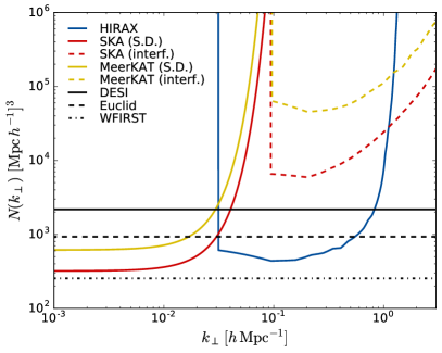
Figure 13: Noise power spectrum at $z=1.2$ as a function of transverse wavenumber $k_{\perp}$ for HIRAX (blue), SKA (red) and MeerKAT (yellow). The curves for SKA and MeerKAT are separated into single-dish (solid) and interferometer (dashed). The shot-noise levels for the spectroscopic surveys DESI, Euclid and WFIRST at the same redshift are shown as black solid, dashed and dot-dashed respectively.

In temperature units, the noise variance per visibility is given by $\langle|V({\bf u})|^{2}\rangle=[\lambda^{2}T_{\rm sys}/(A_{e}\sqrt{\Delta\nu\,t_{p}})]^{2}$. Relating baselines to Fourier coefficients as ${\bf u}={\bf l}/(2\pi)$ and recalling the definition of power spectrum (Eq. 30), the noise power spectrum in temperature is then given by

$$P_{T}({\bf l})=\frac{\lambda^{2}T_{\rm sys}^{2}N_{p}}{A_{e}^{2}\,\Delta\nu\,t_{\rm tot}\,n({\bf u}={\bf l}/(2\pi))},$$ (38)

where $N_{p}$ is the total number of pointings. Relating $n({\bf u})$ to the number density of physical baselines, and defining $N_{p}\Omega_{p}\equiv 4\pi f_{\rm sky}$ we recover the expression for the noise power spectrum of interferometers in Eq. 6.

Comparison with spectroscopic surveys

Converting the angular maps in different frequency channels into a three-dimensional map of the HI overdensity, we can relate the 3D noise power spectrum to its angular counterpart as:

$$P_{3D}({\bf k}_{\parallel},{\bf k}_{\perp})=\frac{c[(1+z)r(z)]^{2}}{\nu_{21}H(z)T^{2}_{\rm HI}(z)}P_{T}({\bf l}\equiv r{\bf k}_{\perp}),$$ (39)

where $r$ is the comoving angular diameter distance to redshift $z$ and $T_{\rm HI}$ is the average 21cm temperature. This can then be directly compared with the shot-noise power spectrum of spectroscopic surveys, given by $P^{3D}=1/\bar{n}$, where $\bar{n}$ is the 3D density of sources. The left panel of Figure 13 shows the 3D noise power spectrum at $z\sim 1.2$ as a function of the transverse wavenumber ${\bf k}_{\perp}$ for the three IM experiments (HIRAX, SKA and MeerKAT) and the three next-generation spectroscopic surveys (DESI, Euclid and WFIRST) considered here.

References

- Newman (2008) J. A. Newman, Astrophys. J. 684, 88-101 (2008), arXiv:0805.1409 .
- Benjamin et al. (2010) J. Benjamin, L. van Waerbeke, B. Ménard, and M. Kilbinger, MNRAS 408, 1168 (2010), arXiv:1002.2266 [astro-ph.CO] .
- Matthews and Newman (2010) D. J. Matthews and J. A. Newman, Astrophys. J. 721, 456 (2010), arXiv:1003.0687 [astro-ph.CO] .
- Schmidt et al. (2013) S. J. Schmidt, B. Ménard, R. Scranton, C. Morrison, and C. K. McBride, MNRAS 431, 3307 (2013), arXiv:1303.0292 .
- Ménard et al. (2013) B. Ménard, R. Scranton, S. Schmidt, C. Morrison, D. Jeong, T. Budavari, and M. Rahman, ArXiv e-prints (2013), arXiv:1303.4722 .
- van Daalen and White (2017) M. P. van Daalen and M. White, ArXiv e-prints (2017), arXiv:1703.05326 .
- Rahman et al. (2016a) M. Rahman, A. J. Mendez, B. Ménard, R. Scranton, S. J. Schmidt, C. B. Morrison, and T. Budavári, MNRAS 460, 163 (2016a), arXiv:1512.03057 .
- Choi et al. (2016) A. Choi, C. Heymans, C. Blake, H. Hildebrandt, C. A. J. Duncan, T. Erben, R. Nakajima, L. Van Waerbeke, and M. Viola, MNRAS 463, 3737 (2016), arXiv:1512.03626 .
- Scottez et al. (2016) V. Scottez, Y. Mellier, B. R. Granett, T. Moutard, M. Kilbinger, et al., MNRAS 462, 1683 (2016), arXiv:1605.05501 .
- Rahman et al. (2016b) M. Rahman, B. Ménard, and R. Scranton, MNRAS 457, 3912 (2016b), arXiv:1508.03046 .
- Johnson et al. (2017) A. Johnson, C. Blake, A. Amon, T. Erben, K. Glazebrook, et al., MNRAS 465, 4118 (2017), arXiv:1611.07578 .
- Battye et al. (2004) R. A. Battye, R. D. Davies, and J. Weller, Mon. Not. Roy. Astron. Soc. 355, 1339 (2004), arXiv:astro-ph/0401340 [astro-ph] .
- McQuinn et al. (2006) M. McQuinn, O. Zahn, M. Zaldarriaga, L. Hernquist, and S. R. Furlanetto, Astrophys. J. 653, 815 (2006), astro-ph/0512263 .
- Chang et al. (2008) T.-C. Chang, U.-L. Pen, J. B. Peterson, and P. McDonald, Phys. Rev. Lett. 100, 091303 (2008), arXiv:0709.3672 [astro-ph] .
- Wyithe and Loeb (2008) J. S. B. Wyithe and A. Loeb, M.N.R.A.S. 383, 606 (2008).
- Loeb and Wyithe (2008) A. Loeb and J. S. B. Wyithe, Physical Review Letters 100, 161301 (2008), arXiv:0801.1677 .
- Peterson et al. (2009) J. B. Peterson, R. Aleksan, R. Ansari, et al., in astro2010: The Astronomy and Astrophysics Decadal Survey, ArXiv Astrophysics e-prints, Vol. 2010 (2009) p. 234, arXiv:0902.3091 [astro-ph.IM] .
- Bagla et al. (2010) J. Bagla, N. Khandai, and K. K. Datta, Mon. Not. Roy. Astron. Soc. 407, 567 (2010), arXiv:0908.3796 [astro-ph.CO] .
- Battye et al. (2013) R. A. Battye, I. W. A. Browne, C. Dickinson, G. Heron, B. Maffei, and A. Pourtsidou, M.N.R.A.S. 434, 1239 (2013), arXiv:1209.0343 [astro-ph.CO] .
- Masui et al. (2013) K. W. Masui, E. R. Switzer, N. Banavar, K. Bandura, C. Blake, et al., ApJL 763, L20 (2013), arXiv:1208.0331 [astro-ph.CO] .
- Switzer et al. (2013) E. R. Switzer, K. W. Masui, K. Bandura, L.-M. Calin, T.-C. Chang, et al., MNRAS 434, L46 (2013), arXiv:1304.3712 [astro-ph.CO] .
- Bull et al. (2015) P. Bull, P. G. Ferreira, P. Patel, and M. G. Santos, Astrophys. J. 803, 21 (2015), arXiv:1405.1452 .
- Fonseca et al. (2017) J. Fonseca, R. Maartens, and M. G. Santos, MNRAS 466, 2780 (2017), arXiv:1611.01322 .
- Newburgh et al. (2016) L. B. Newburgh, K. Bandura, M. A. Bucher, T.-C. Chang, H. C. Chiang, et al., in Society of Photo-Optical Instrumentation Engineers (SPIE) Conference Series, Proceedings of the SPIE, Vol. 9906 (2016) p. 99065X, arXiv:1607.02059 [astro-ph.IM] .
- Santos et al. (2015) M. Santos, P. Bull, D. Alonso, S. Camera, P. Ferreira, et al., Advancing Astrophysics with the Square Kilometre Array (AASKA14) , 19 (2015), arXiv:1501.03989 .
- McQuinn and White (2013) M. McQuinn and M. White, MNRAS 433, 2857 (2013), arXiv:1302.0857 .
- Jasche and Wandelt (2012) J. Jasche and B. D. Wandelt, MNRAS 425, 1042 (2012), arXiv:1106.2757 .
- Alonso and Ferreira (2015) D. Alonso and P. G. Ferreira, Phys. Rev. D 92, 063525 (2015), arXiv:1507.03550 .
- Gabasch et al. (2006) A. Gabasch, U. Hopp, G. Feulner, R. Bender, S. Seitz, et al., A&A 448, 101 (2006), astro-ph/0510339 .
- Blanton and Roweis (2007) M. R. Blanton and S. Roweis, Astron. Journal 133, 734 (2007), astro-ph/0606170 .
- LSST Collaboration et al. (2009) LSST Collaboration et al., arXiv e-prints (2009), arXiv:0912.0201 [astro-ph.IM] .
- Weinberg et al. (2004) D. H. Weinberg, R. Davé, N. Katz, and L. Hernquist, Astrophys. J. 601, 1 (2004), astro-ph/0212356 .
- Battye et al. (2012) R. A. Battye, M. L. Brown, I. W. A. Browne, R. J. Davis, P. Dewdney, C. Dickinson, G. Heron, B. Maffei, A. Pourtsidou, and P. N. Wilkinson, ArXiv e-prints (2012), arXiv:1209.1041 [astro-ph.CO] .
- Newburgh et al. (2014) L. B. Newburgh, G. E. Addison, M. Amiri, K. Bandura, J. R. Bond, et al., in Ground-based and Airborne Telescopes V, Proceedings of the SPIE, Vol. 9145 (2014) p. 91454V, arXiv:1406.2267 [astro-ph.IM] .
- Bigot-Sazy et al. (2016) M.-A. Bigot-Sazy, Y.-Z. Ma, R. A. Battye, I. W. A. Browne, T. Chen, et al., in Frontiers in Radio Astronomy and FAST Early Sciences Symposium 2015, Astronomical Society of the Pacific Conference Series, Vol. 502, edited by L. Qain and D. Li (2016) p. 41, arXiv:1511.03006 .
- Chen (2011) X. Chen, Scientia Sinica Physica, Mechanica & Astronomica 41, 1358 (2011).
- Santos et al. (2005) M. G. Santos, A. Cooray, and L. Knox, Astrophys. J. 625, 575 (2005), astro-ph/0408515 .
- Wolz et al. (2014) L. Wolz, F. B. Abdalla, C. Blake, J. R. Shaw, E. Chapman, and S. Rawlings, MNRAS 441, 3271 (2014), arXiv:1310.8144 .
- Shaw et al. (2015) J. R. Shaw, K. Sigurdson, M. Sitwell, A. Stebbins, and U.-L. Pen, Phys. Rev. D 91, 083514 (2015), arXiv:1401.2095 .
- Alonso et al. (2015) D. Alonso, P. Bull, P. G. Ferreira, and M. G. Santos, MNRAS 447, 400 (2015), arXiv:1409.8667 .
- Planck Collaboration et al. (2016) Planck Collaboration et al., A&A 594, A10 (2016), arXiv:1502.01588 .
- Levi et al. (2013) M. Levi, C. Bebek, T. Beers, R. Blum, R. Cahn, et al., ArXiv e-prints (2013), arXiv:1308.0847 [astro-ph.CO] .
- Font-Ribera et al. (2014) A. Font-Ribera, P. McDonald, N. Mostek, B. A. Reid, H.-J. Seo, and A. Slosar, JCAP 5, 023 (2014), arXiv:1308.4164 .
- Laureijs et al. (2011) R. Laureijs, J. Amiaux, S. Arduini, J. . Auguères, J. Brinchmann, et al., ArXiv e-prints (2011), arXiv:1110.3193 [astro-ph.CO] .
- Spergel et al. (2013) D. Spergel, N. Gehrels, J. Breckinridge, M. Donahue, A. Dressler, et al., ArXiv e-prints (2013), arXiv:1305.5422 [astro-ph.IM] .
- Tegmark et al. (1998) M. Tegmark, A. J. S. Hamilton, M. A. Strauss, M. S. Vogeley, and A. S. Szalay, Astrophys. J. 499, 555 (1998), astro-ph/9708020 .
- Bond et al. (1998) J. R. Bond, A. H. Jaffe, and L. Knox, Phys. Rev. D 57, 2117 (1998), astro-ph/9708203 .
- Newman et al. (2015) J. A. Newman, A. Abate, F. B. Abdalla, S. Allam, S. W. Allen, et al., Astroparticle Physics 63, 81 (2015), arXiv:1309.5384 .
- de Putter et al. (2014) R. de Putter, O. Doré, and S. Das, Astrophys. J. 780, 185 (2014), arXiv:1306.0534 .
- The Dark Energy Survey Collaboration (2005) The Dark Energy Survey Collaboration, ArXiv Astrophysics e-prints (2005), astro-ph/0510346 .
- Camera et al. (2013) S. Camera, M. G. Santos, P. G. Ferreira, and L. Ferramacho, Physical Review Letters 111, 171302 (2013), arXiv:1305.6928 [astro-ph.CO] .
- Jelić et al. (2010) V. Jelić, S. Zaroubi, P. Labropoulos, G. Bernardi, A. G. de Bruyn, and L. V. E. Koopmans, MNRAS 409, 1647 (2010), arXiv:1007.4135 .
- Datta et al. (2010) A. Datta, J. D. Bowman, and C. L. Carilli, Astrophys. J. 724, 526 (2010), arXiv:1005.4071 .
- Vedantham et al. (2012) H. Vedantham, N. Udaya Shankar, and R. Subrahmanyan, Astrophys. J. 745, 176 (2012), arXiv:1106.1297 [astro-ph.IM] .
- Liu et al. (2014) A. Liu, A. R. Parsons, and C. M. Trott, Phys. Rev. D 90, 023019 (2014), arXiv:1404.4372 .
- Seo and Hirata (2016) H.-J. Seo and C. M. Hirata, MNRAS 456, 3142 (2016), arXiv:1508.06503 .
- Parsons et al. (2012) A. R. Parsons, J. C. Pober, J. E. Aguirre, C. L. Carilli, D. C. Jacobs, and D. F. Moore, Astrophys. J. 756, 165 (2012), arXiv:1204.4749 [astro-ph.IM] .
- Pober et al. (2014) J. C. Pober, A. Liu, J. S. Dillon, J. E. Aguirre, J. D. Bowman, R. F. Bradley, C. L. Carilli, D. R. DeBoer, J. N. Hewitt, D. C. Jacobs, M. McQuinn, M. F. Morales, A. R. Parsons, M. Tegmark, and D. J. Werthimer, Astrophys. J. 782, 66 (2014), arXiv:1310.7031 .
- Abazajian et al. (2016) K. N. Abazajian, P. Adshead, Z. Ahmed, S. W. Allen, D. Alonso, et al., ArXiv e-prints (2016), arXiv:1610.02743 .
- Calabrese et al. (2016) E. Calabrese, D. Alonso, and J. Dunkley, ArXiv e-prints (2016), arXiv:1611.10269 .
- Baxter et al. (2016) E. Baxter, J. Clampitt, T. Giannantonio, S. Dodelson, B. Jain, et al., MNRAS 461, 4099 (2016), arXiv:1602.07384 .
- Takahashi et al. (2012) R. Takahashi, M. Sato, T. Nishimichi, A. Taruya, and M. Oguri, Astrophys. J. 761, 152 (2012), arXiv:1208.2701 .
- Blas et al. (2011) D. Blas, J. Lesgourgues, and T. Tram, JCAP 7, 034 (2011), arXiv:1104.2933 .
- Di Dio et al. (2013) E. Di Dio, F. Montanari, J. Lesgourgues, and R. Durrer, JCAP 11, 044 (2013), arXiv:1307.1459 .