CCL: Cross-modal Correlation Learning with Multi-grained Fusion by Hierarchical Network

Abstract

Cross-modal retrieval has become a highlighted research topic for retrieval across multimedia data such as image and text. A two-stage learning framework is widely adopted by most existing methods based on Deep Neural Network (DNN): The first learning stage is to generate separate representation for each modality, and the second learning stage is to get the cross-modal common representation. However, the existing methods have three limitations: (1) In the first learning stage, they only model intra-modality correlation, but ignore inter-modality correlation with rich complementary context. (2) In the second learning stage, they only adopt shallow networks with single-loss regularization, but ignore the intrinsic relevance of intra-modality and inter-modality correlation. (3) Only original instances are considered while the complementary fine-grained clues provided by their patches are ignored. For addressing the above problems, this paper proposes a cross-modal correlation learning (CCL) approach with multi-grained fusion by hierarchical network, and the contributions are as follows: (1) In the first learning stage, CCL exploits multi-level association with joint optimization to preserve the complementary context from intra-modality and inter-modality correlation simultaneously. (2) In the second learning stage, a multi-task learning strategy is designed to adaptively balance the intra-modality semantic category constraints and inter-modality pairwise similarity constraints. (3) CCL adopts multi-grained modeling, which fuses the coarse-grained instances and fine-grained patches to make cross-modal correlation more precise. Comparing with 13 state-of-the-art methods on 6 widely-used cross-modal datasets, the experimental results show our CCL approach achieves the best performance.

I Introduction

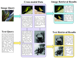
Figure 1: An example of cross-modal retrieval with image and text, which can present retrieval results with different modalities.

With rapid development of computer science and technology, multimedia data including image, video, text and audio, has been emerging on the Internet and reshaping people’s life. Consequently, multimedia retrieval has been an essential technique with wide applications, such as search engine and multimedia data management. The traditional retrieval methods mainly focus on single-modal scenario [1, 2], which provides retrieval results of the same single modality with query, such as image retrieval and text retrieval. Furthermore, some methods attempt to address the retrieval problem where multimedia data exists as tight combination [3, 4]. But the major limitation of these methods is that the retrieval results must share the same modality combination with user’s queries, e.g. retrieving image/text pairs with the query of an image/text pair. They cannot directly measure the similarity between different modalities, which restricts the retrieval flexibility.

Cross-modal retrieval is a relatively new retrieval paradigm, which can perform retrieval across multimedia data. For example, if someone is interested in canary, he can submit one image query, and then get relevant multimedia information, including text descriptions, image samples, video introductions, audio clips and so on. Figure 1 is an example of cross-modal retrieval with image and text. Compared with single-modal retrieval, cross-modal retrieval can provide more flexible and useful retrieval experience to show rich multimedia search results. The key problem of cross-modal retrieval is that the distribution and representation of different modalities are inconsistent, and such “heterogeneity gap” makes it hard to measure the cross-modal similarity.

For bridging “heterogeneity gap”, most existing methods are proposed to learn a common space for different modalities. These methods like [5, 6, 7] aim to project the features from single-modal space into cross-modal common space and get common representation for similarity measure. The common representation is usually generated following principles such as maximizing cross-modal pairwise correlation [5], maximizing classification accuracy in the common space [8], etc. According to the different adopted models, existing methods can be divided into two major ways. The first is to learn linear projections in traditional frameworks, like Canonical Correlation Analysis (CCA) [5] and graph-based methods [8]. However, their performance is limited by the traditional framework, which cannot capture the complex cross-modal correlation with high non-linearity. As indicated in [9], although some kernel based methods have the ability of learning non-linear representation, the learned representation is limited due to the fixed kernel. With the great progress by deep learning in single-modal scenario such as image classification, there arises the second way for common representation learning, which takes DNN as the basic model. These methods take the advantage of DNN’s strong ability of non-linear modeling for analyzing complex cross-modal correlation [10, 11, 12], which avoid the aforementioned problems of nonparametric models in traditional methods to learn more flexible non-linear representation.

DNN-based methods for common representation learning can be mainly divided into two stages: The first learning stage is to generate separate representation for each modality, and the second learning stage is to learn common representation by exploiting cross-modal correlation. However, in the first learning stage, these methods only model intra-modality correlation to obtain separate representation [13], but ignore the intrinsic correlation within inter-modality. In the second learning stage, existing methods learn common representation with single-loss regularization [10], which ignore the intrinsic relevance of intra-modality and inter-modality correlation. Besides, existing methods [10, 11] only extract separate representation from the original instances, but ignore the rich complementary fine-grained clues provided by their patches. The great progress of fine-grained image classification [14] shows the effectiveness of modeling fine-grained patches that contain discriminative local parts in single-modal scenario. It can also make great contribution to cross-modal retrieval because fine-grained correlation between patches of different modalities can provide more precise and complementary cross-modal correlation to the original instances.

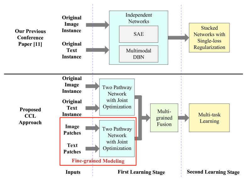
Figure 2: The schematic diagram to show the difference between the proposed CCL approach and our previous conference paper [11].

For addressing the above issues, this paper proposes a cross-modal correlation learning (CCL) approach with multi-grained fusion by hierarchical network. Its main advantages and contributions can be summarized as follows:

• Cross-modal correlation exploiting. In the first learning stage for separate representation of each modality, existing methods [10, 13] only model intra-modality correlation but ignore inter-modality correlation. Actually, inter-modality correlation can provide rich complementary context to intra-modality one for learning better separate representation. So we employ multi-level association with joint optimization by maximizing intra-modality and inter-modality correlation simultaneously, which can capture the important hints from cross-modal correlation to boost common representation learning.

• Multi-task learning. In the second learning stage for common representation of different modalities, existing methods only adopt shallow networks with single-loss regularization [9, 12], which ignore the intrinsic relevance of intra-modality and inter-modality correlation, so cannot effectively exploit and balance them to improve generalization performance. So we design a multi-task learning strategy to adaptively balance intra-modality semantic category constraints and inter-modality pairwise similarity constraints, and make them mutually boost each other by fully exploiting their intrinsic relevance.

• Multi-grained fusion. The patches contain complementary fine-grained clues to the original instances, which are ignored by the existing methods [11, 15]. So we construct a multi-pathway network to fuse the multi-grained information in parallel by modeling the joint distributions, which can exploit and integrate the coarse-grained instances and fine-grained patches to make cross-modal correlation more precise.

The main differences between the proposed CCL approach and our previous conference paper CMDN [11] can be summarized as the following three aspects: (1) Our proposed CCL approach jointly employs the coarse-grained instances and fine-grained patches for multi-grained fusion to learn more precise cross-modal correlation and boost cross-modal retrieval. While CMDN only uses the original coarse-grained instances, which ignores complementary fine-grained clues provided by their patches. (2) Our proposed CCL approach adopts a multi-task learning strategy to adaptively balance intra-modality semantic category constraints and inter-modality pairwise similarity constraints. While CMDN only adopts single-loss regularization, which cannot effectively exploit and balance the above constraints to improve generalization performance. (3) Our proposed CCL approach learns the separate representation in the first learning stage through one linked two-pathway network by jointly optimizing the intrinsic intra-modality and inter-modality correlation, which can fully capture these complementary hints simultaneously from cross-modal correlation. While CMDN learns the intra-modality and inter-modality separate representations respectively by two independent networks, which cannot effectively exploit the intrinsic relationship between these two kinds of complementary information. A schematic diagram in Figure 2 intuitively demonstrates the differences between CCL and CMDN. To the best of our knowledge, the proposed CCL approach is the first to simultaneously model intra-modality and inter-modality correlation in both two learning stages, and employ the coarse-grained instances and fine-grained patches, which can learn more precise cross-modal correlation. Comparing with 13 state-of-the-art methods on 6 widely-used datasets, the effectiveness of our CCL approach is verified from the comprehensive experimental results.

The rest of this paper is organized as follows: Related works on cross-modal retrieval are briefly reviewed in Section II. Section III presents our proposed CCL approach. Section IV introduces the experiments as well as the results analysis. Finally Section V concludes this paper.

II Related Works

In this section, we briefly review the representative methods of cross-modal retrieval, which are divided into two categories: Traditional methods and DNN-based methods.

II-A Traditional Cross-modal Retrieval Methods

As for the traditional cross-modal retrieval methods, one representative method is Canonical Correlation Analysis (CCA) [16]. Given a set of pairwise cross-modal data (such as image/text pairs), CCA learns a common space where the two modalities have maximum correlation. Mapping matrices can be learned by CCA to project the features of different modalities into a lower-dimensional common space, and then common representation is obtained. CCA is widely used to model the multimodal data [17, 18, 19] and also has many extensions and varieties [5, 20]. For example, Rasiwasia et al. [5] attempt to combine category information with CCA, and Multi-view CCA [20] extends CCA with the third view of high-level semantics. Similar to CCA, Li et al. [21] propose Cross-modal Factor Analysis (CFA) which also models the pairwise cross-modal correlation, but learns the projections by minimizing the Frobenius norm between pairwise data in common space. Ranjan et al. [22] propose multi-label CCA as an extension of CCA, which does not rely on the pairwise correspondence but considers the high-level semantic information in the form of multi-label annotations. Tran et al. [23] embed the projections of visual and textual features into a local context that reflects the data distribution in the common space. Besides, Hua et al. [24] propose a cross-modal correlation method with adaptive hierarchical semantic aggregation, which constructs a set of local projections and probabilistic membership functions for image and text.

More recently, some methods apply semi-supervised learning and graph regularization into cross-modal common representation learning. For example, Joint Graph Regularized Heterogeneous Metric Learning (JGRHML) [25] proposed by Zhai et al. adopt metric learning and graph regularization to learn the project matrices, which constructs a joint graph regularization term using the data in the learned metric space. Joint Representation Learning (JRL) [8] is proposed to construct a separate graph for each modality to learn a common space, which uses semantic information with semi-supervised regularization and sparse regularization. Wang et al. [26] adopt multimodal graph regularization term on the projected data with an iterative algorithm, which aims to preserve inter-modality and intra-modality similarity relationships.

II-B DNN-based Cross-modal Retrieval Methods

Deep learning has shown its strong power in modeling non-linear correlation, and achieved state-of-the-art performance in some applications of single-modal scenario, such as object detection [27, 28] and image/video classification [29, 30]. Inspired by this, researchers attempt to model the complex cross-modal correlation with DNN, and the existing methods can be divided into two learning stages. The first learning stage is to generate separate representation for each modality. And the second learning stage is to learn common representation, which is the main focus of most existing methods based on DNN [10, 13]. We briefly introduce some representative cross-modal retrieval methods based on DNN as follows:

The Multimodal Deep Belief Network (Multimodal DBN) [13] is proposed to learn common representation for the data of different modalities. In the first learning stage for separate representation, it adopts a two-layer DBN for each modality to model the distribution of original features, where Gaussian Restricted Boltzmann Machine (RBM) is adopted for image instances, while Replicated Softmax model [31] is used for text instances. RBM has several visible units $v$ and hidden units $h$, which is the basic component of DBN, and the energy function and joint distribution are defined as follows:

$$E(v,h;\theta)=-a^{\mathrm{T}}v-b^{\mathrm{T}}h-v^{\mathrm{T}}Wh$$ (1)

$$P(v,h;\theta)=\frac{1}{Z(\theta)}exp(-E(v,h;\theta))$$ (2)

where $\theta$ is the collection of three parameters $a,b,W$ ($a,b$ are the bias parameters and $W$ is the weight parameter) and $Z(\theta)$ is the normalizing constant. Then in the second learning stage, multimodal DBN applies a joint RBM on top of the two separate DBNs and combines them by modeling the joint distribution of data with different modalities to get common representation.

The Bimodal Autoencoders (Bimodal AE) [15] proposed by Ngiam et al. is based on deep autoencoder network, which is actually an extension of RBM for modeling multiple modalities. It has two subnetworks to learn separate representation in the first learning stage, and then the two subnetworks are linked at the shared joint layer to generate common representation in the second learning stage. Bimodal AE reconstructs different modalities such as image and text jointly by minimizing the reconstruction error between the original feature and reconstructed representation. Bimodal AE can learn high-order correlation between multiple modalities and preserve the reconstruction information at the same time.

Correspondence Autoencoder (Corr-AE) [10] first adopts DBN to generate separate representation in the first learning stage. And then in the second learning stage, it jointly models the correlation and reconstruction information with two subnetworks linked at the code layer, which minimizes a combination of representation learning error within each modality and correlation learning error between different modalities. Corr-AE, which only reconstructs the input itself, has two similar structures for extension: Corr-Cross-AE and Corr-Full-AE. Corr-Cross-AE attempts to reconstruct the input from different modalities, while Corr-Full-AE can reconstruct both the input itself and the input of different modalities.

Cross-media Multiple Deep Networks (CMDN) (our previous conference paper [11] ) jointly models the complementary intra-modality and inter-modality correlation between different modalities in the first learning stage. It should be noted that two independent networks are adopted in the first learning stage of CMDN. Specifically, Stacked Autoencoder (SAE) [32] is used to model intra-modality correlation, while the Multimodal DBN is used to capture inter-modality correlation. In the second learning stage, a hierarchical learning strategy is adopted to learn the cross-modal correlation with a two-level network, and common representation is learned by a stacked network based on Bimodal AE. The above DNN-based methods have three limitations in summary as follows.

1) In the first learning stage, the existing methods as [10, 13] only model intra-modality correlation to generate separate representation, but ignore the rich complementary context provided by inter-modality correlation, which should be preserved for learning better separate representation. Although our previous work [11] also considers intra-modality and inter-modality correlation in the first learning stage, it adopts two independent networks to model each of them respectively, which cannot fully exploit the complex relationship between intra-modality and inter-modality correlation. While our proposed CCL approach models the two kinds of complementary information by jointly optimizing intra-modality reconstruction information and inter-modality pairwise similarity.

2) In the second learning stage, existing methods learn common representation by adopting shallow network architectures with single-loss regularization [9, 12]. However, the intra-modality and inter-modality correlation has intrinsic relevance, and such relevance is ignored by the single-loss regularization, which leads to inability for improving generalization performance. Multi-task learning (MTL) framework has been proposed to enhance the generalization ability by constructing a series of learning processes, which are relevant to each other and can mutually boost each other. Recently, extensive research works attempt to apply multi-task learning into deep architecture. DeepID2 [33] simultaneously learns face identification and verification as two learning tasks to achieve better accuracy of face recognition. Ren et al. [34] propose Faster R-CNN, which also consists of two learning tasks as the object bound and objectness score prediction, and boosts the object detection accuracy. Besides, a joint multi-task learning algorithm [35] is proposed to predict attributes in images. However, most of the research efforts have focused on the single-modal scenario. Inspired by the above methods, we apply multi-task learning to perform common representation learning. It aims to balance intra-modality semantic category constraints and inter-modality pairwise similarity constraints to further improve the accuracy of cross-modal retrieval.

3) Furthermore, only the original instances are considered by the existing methods based on DNN [10, 11, 15]. Although patches have been exploited in some traditional methods as [36], the accuracies of these methods are limited because of the traditional framework, which cannot effectively model the complex correlation between the patches with high non-linearity. Our proposed CCL approach can fully exploit the coarse-grained instances as well as the rich complementary fine-grained patches by DNN, and fuse the multi-grained information to capture the intrinsic correlation between different modalities.

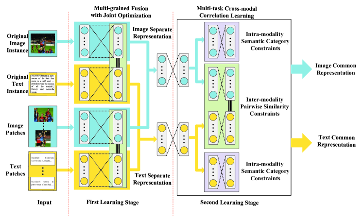
Figure 3: An overview of our CCL approach with two learning stages: In the first learning stage, we learn separate representation by simultaneously modeling intra-modality and inter-modality correlation, which integrates the original instances and their patches in parallel. Then in the second learning stage, we adopt a multi-task learning strategy to adaptively balance intra-modality and inter-modality correlation, which leads to more accurate common representation.

III Our CCL Approach

As shown in Figure 3, CCL simultaneously models intra-modality and inter-modality correlation in both two learning stages, and employs the coarse-grained instances and fine-grained patches, which can learn more precise cross-modal correlation.

The formal definition will first be given. The multimodal dataset consists of two modalities with $m$ image instances and $n$ text instances, which is denoted as $D=\left\{D^{(i)},D^{(t)}\right\}$. Here $D^{(i)}=\left\{x_{p}^{(i)},y_{p}^{(i)}\right\}_{p=1}^{m}$ denotes the data of image modality, where the $p$-th image instance is denoted as $x_{p}^{(i)}\in\mathbb{R}^{d^{(i)}}$ with its corresponding label $y_{p}^{(i)}$ and the dimensional number $d^{(i)}$. $D^{(t)}=\left\{x_{q}^{(t)},y_{q}^{(t)}\right\}_{q=1}^{n}$ denotes the data of text modality, where the text instance is defined as $x_{q}^{(t)}\in\mathbb{R}^{d^{(t)}}$ with the label $y_{q}^{(t)}$ and the dimensional number $d^{(t)}$. Besides, the pairwise correspondence is denoted as $(x_{p}^{(i)},x_{p}^{(t)})$, which means that the two instances of different modalities co-exist to describe the relevant semantics.

III-A First Learning Stage: Multi-grained Fusion with Joint Optimization

In the first learning stage, we construct a multi-pathway network, which aims to obtain separate representations from both the original instances as well as their patches of each modality in parallel, and capture intra-modality and inter-modality correlation with joint optimization at the same time.

III-A1 Coarse-grained learning with original instances

A two-pathway network structure is adopted to model the image and text instances. First, two types of Deep Belief Network (DBN) [37] are used to model the distribution over the features of each modality, where Gaussian Restricted Boltzmann Machine (RBM) [38] is adopted to model the image instances and Replicated Softmax model [31] is adopted for text instances. We define the probability functions of each DBN as follows:

$$P(v_{i})=\sum_{h^{(1)},h^{(2)}}P(h^{(2)},h^{(1)})P(v_{i}|h^{(1)})$$ (3)

$$P(v_{t})=\sum_{h^{(1)},h^{(2)}}P(h^{(2)},h^{(1)})P(v_{t}|h^{(1)})$$ (4)

where the two hidden layers of DBN are denoted as $h^{(1)}$ and $h^{(2)}$, while $v_{i}$ is for image input and $v_{t}$ is for text input. The outputs of two DBNs can preserve the original characteristic of each modality with high-level semantic information, which are denoted as $Q^{(i)}$ and $Q^{(t)}$.

Then we simultaneously model intra-modality and inter-modality correlation by joint optimization for $Q^{(i)}$ of image instance and $Q^{(t)}$ of text instance. Compared with our previous CMDN method [11], which adopts two independent networks for intra-modality and inter-modality to learn separate representation, a two-pathway network linked at the top code layer is constructed. We minimize the following loss function to jointly optimize the reconstruction learning error and correlation learning error:

$$L(Q^{(i)},Q^{(t)})= L_{r}(Q^{(i)},Q_{r}^{(i)})+L_{r}(Q^{(t)},Q_{r}^{(t)})$$

$$+L_{c}(Q^{(i)},Q^{(t)})$$ (5)

$$L_{r}(Q^{(k)},Q_{r}^{(k)}) =\left\|Q^{(k)}-Q_{r}^{(k)}\right\|^{2},k=i,t$$ (6)

$$L_{c}(Q^{(i)},Q^{(t)}) =\left\|Q^{(i)}-Q^{(t)}\right\|^{2}$$ (7)

where $Q_{r}^{(i)}$ and $Q_{r}^{(t)}$ denote the reconstruction representations of image and text, and $L_{r}$ in Eq.(6) represents the loss of reconstruction learning error, which aims to minimize the L2 distance between the input and reconstruction representation of each modality. $L_{c}$ in Eq.(7) is for correlation learning error to minimize the L2 distance between the instances of different modalities. Thus, we can get the coarse-grained representations with both intra-modality and inter-modality correlation for the original instances of different modalities, which are denoted as $T_{origin}^{(i)}$ and $T_{origin}^{(t)}$.

III-A2 Fine-grained learning with patches

We first divide each original image and text instance into several patches, which is showed in Figure 4. Specifically, we adopt selective search [39] to extract region proposals, which can find the visual objects in the image instance containing rich fine-grained information. For text, the segmentation is performed according to the form of text, where the text is divided into paragraphs, sentences or words. Similar with the original instances, a two-pathway network structure is constructed with two types of DBN adopted over the features extracted from the patches of image and text. For the patches within one original instance, average fusion is adopted to combine their representations obtained from DBN, and the results are denoted as $U^{(i)}$ and $U^{(t)}$. Then we link the two-pathway network at the code layer, and minimize the following loss function to model intra-modality and inter-modality correlation with joint optimization:

$$L(U^{(i)},U^{(t)})= L_{r}(U^{(i)},U_{r}^{(i)})+L_{r}(U^{(t)},U_{r}^{(t)})$$

$$+L_{c}(U^{(i)},U^{(t)})$$ (8)

where the loss of reconstruction learning error is represented as $L_{r}$, and the loss of correlation learning error is denoted as $L_{c}$. They have similar definition with Eq.(6) and Eq.(7). Therefore, the fine-grained representations denoted as $T_{patch}^{(i)}$ and $T_{patch}^{(t)}$ are obtained from patches of different modalities, which preserve fine-grained intra-modality and inter-modality correlation.

III-A3 Multi-grained Fusion

We adopt a joint RBM for each modality to fuse the coarse-grained and fine-grained representations obtained from both the original instances ($T_{origin}^{(i)}$, $T_{origin}^{(t)}$) and their patches ($T_{patch}^{(i)}$, $T_{patch}^{(t)}$). And the joint distribution is defined as follows:

$$P(v_{1},v_{2})=\sum_{h_{1}^{(1)},h_{2}^{(1)},h^{(2)}}P(h_{1}^{(1)},h_{2}^{(1)},h^{(2)})\times$$

$$\sum_{h_{1}^{(1)}}P(v_{1}\mid h_{1}^{(1)})\times\sum_{h_{2}^{(1)}}P(v_{2}\mid h_{2}^{(1)})$$ (9)

where the two types of intermediate representation $T_{origin}^{(i)}$ and $T_{patch}^{(i)}$ for image instances are denoted as $v_{1}$ and $v_{2}$. Thus, this joint distribution is collected as separate representation for image, which can also be adopted on the two intermediate representations of text instances $T_{origin}^{(t)}$ and $T_{patch}^{(t)}$ to generate separate representation for text. The obtained separate representations for image and text are denoted as $S^{(i)}$ and $S^{(t)}$, which capture the intrinsic correlation and rich complementary information contained in both original instances and their patches of each modality.

Figure 4: Examples for the generation of fine-grained patches.

III-B Second Learning Stage: Multi-task Cross-modal Correlation Learning

In the second learning stage for generating common representation, as shown in the right of Figure 3, we propose a multi-task learning framework to model intra-modality semantic category constraints and inter-modality pairwise similarity constraints as two loss branches. The former aims to improve the semantic discriminative ability in the high-level common space, while the later can capture the intrinsic correlation between different modalities, which leads to more accurate common representation for cross-modal data.

For inter-modality pairwise similarity constraints, most existing works as [10, 11] only focus on pairwise correlation with similar constraints but ignore the semantically dissimilar constraints. Thus we model the pairwise similar and dissimilar constraints between different modalities with a contrastive loss, which has the following considerations: Image and text instances with the same label should be similar and the distance between them should be minimized, while on the contrary, image and text instances which have different labels should be dissimilar and their distance should be maximized. Specifically, a neighborhood graph $G=(V,E)$ is constructed in a mini-batch of data for one iteration, where the vertices $V$ represent the image and text instances, and $E$ is the similarity matrix between data of two modalities according to their labels, which is defined as follows:

$$E(p,q)=\begin{cases}1&:y_{p}^{(i)}=y_{q}^{(t)}\\ 0&:y_{p}^{(i)}\neq y_{q}^{(t)}\end{cases}$$ (10)

Thus, the contrastive loss between the image and text pairs is defined to model the pairwise similar and dissimilar constraints as follows:

$$L_{1}(p,q)=\begin{cases}\left\|f(s_{p}^{i})-g(s_{q}^{t})\right\|^{2}&E(p,q)=1\\ max(0,\alpha-\left\|f(s_{p}^{i})-g(s_{q}^{t})\right\|^{2})&E(p,q)=0\end{cases}$$ (11)

where $s_{p}^{i}$ and $s_{q}^{t}$ denote separate representations for image $S^{(i)}$ and text $S^{(t)}$, $f(.)$ and $g(.)$ denote the non-linear mappings respectively for image and text pathways in the multi-task learning network in the second learning stage. Each pathway consists of three fully-connected layers, aiming to convert the separate representations $S^{(i)}$ and $S^{(t)}$ to the final common representations of image and text. The margin parameter is set to be $\alpha$. Then we calculate the derivative of loss function $L_{1}$ in Eq.(11) for positive pair of image $s_{p}^{i}$ and text $s_{q}^{t+}$ where $E(p,q)=1$ as follows:

$$\frac{\partial L_{1}}{\partial f(s_{p}^{i})}=2(f(s_{p}^{i})-g(s_{q}^{t+}))$$ (12)

$$\frac{\partial L_{1}}{\partial g(s_{q}^{t+})}=2(g(s_{q}^{t+})-f(s_{p}^{i}))$$ (13)

then for the negative pair of image $s_{p}^{i}$ and text $s_{q}^{t-}$ where $E(p,q)=0$, the derivative of loss function is calculated as follows:

$$\frac{\partial L_{1}}{\partial f(s_{p}^{i})}=2(g(s_{p}^{i})-f(s_{q}^{t-}))\times J$$ (14)

$$\frac{\partial L_{1}}{\partial g(s_{q}^{t-})}=2(f(s_{q}^{t-})-g(s_{p}^{i}))\times J$$ (15)

where $J=0$ if $\alpha-\left\|f(s_{p}^{i})-g(s_{q}^{t-})\right\|^{2}<=0$, otherwise $J$ is set to be $1$. Therefore, the back-propagation can be applied to update the parameters through the network.

Then, for intra-modality semantic category constraints, a classification process is employed to exploit the intrinsic semantic information within each modality, which can classify data of each modality into one of $n$ categories. Thus, we present intra-modality semantic category constraints as an $n$-way softmax layer, where $n$ is the number of categories. Cross-entropy loss is minimized as follows:

$$L_{2}=-\sum_{i=1}^{n}p_{i}log(\hat{p_{i}})$$ (16)

where the predicted probability distribution is denoted as $\hat{p_{i}}$, and $p_{i}$ is the target probability distribution. By minimizing the above loss function, the semantical discrimination ability of common representation can be greatly enhanced.

Finally, we can obtain the accurate common representations denoted as $M^{(i)}$ and $M^{(t)}$ from the outputs of last fully-connected layer in the multi-task learning network, which can adaptively balance intra-modality semantic category constraints and inter-modality pairwise similarity constraints, and further make them mutually boost each other. For performing the cross-modal retrieval, common representations of each image and text are extracted firstly from the above network structure with the inputs of both original instance and patches, and then the traditional distance metric, such as cosine distance, can be applied to measure the similarity between the instances of different modalities.

TABLE I: The MAP scores of Bi-modal Retrieval for our CCL approach and compared methods on Wikipedia dataset. MAP with two types of image feature are calculated, which are hand-crafted feature and CNN feature, while the text feature is the same.

Method	MAP with hand-crafted feature			MAP with CNN feature
	Image$\rightarrow$Text	Text$\rightarrow$Image	Average	Image$\rightarrow$Text	Text$\rightarrow$Image	Average
Our CCL Approach	0.418	0.359	0.389	0.504	0.457	0.481
CMDN [11]	0.393	0.325	0.359	0.488	0.427	0.458
LGCFL [40]	0.385	0.326	0.356	0.481	0.418	0.450
JRL [8]	0.344	0.277	0.311	0.453	0.400	0.427
DCCA [12]	0.248	0.221	0.235	0.440	0.390	0.415
Corr-AE [10]	0.280	0.242	0.261	0.402	0.395	0.399
Multimodal DBN [13]	0.149	0.150	0.150	0.204	0.183	0.194
Bimodal AE [15]	0.236	0.208	0.222	0.314	0.290	0.302
GMM+HGLMM [19]	0.266	0.233	0.250	0.428	0.396	0.412
Multi-label CCA [22]	0.317	0.266	0.292	0.404	0.366	0.385
MACC [23]	0.255	0.233	0.244	0.470	0.400	0.435
KCCA(Gaussian) [17]	0.245	0.219	0.232	0.326	0.268	0.297
KCCA(Poly) [17]	0.200	0.185	0.193	0.215	0.214	0.215
CFA [21]	0.236	0.211	0.224	0.334	0.297	0.316
CCA [16]	0.203	0.183	0.193	0.258	0.250	0.254

TABLE II: The MAP scores of All-modal Retrieval for our CCL approach and compared methods on Wikipedia dataset. MAP with two types of image feature are calculated, which are hand-crafted feature and CNN feature, while the text feature is the same.

Method	MAP with hand-crafted feature			MAP with CNN feature
	Image$\rightarrow$All	Text$\rightarrow$All	Average	Image$\rightarrow$All	Text$\rightarrow$All	Average
Our CCL Approach	0.331	0.610	0.471	0.422	0.652	0.537
CMDN [11]	0.282	0.592	0.437	0.361	0.637	0.499
LGCFL [40]	0.294	0.576	0.435	0.402	0.601	0.502
JRL [8]	0.281	0.556	0.419	0.381	0.530	0.456
DCCA [12]	0.214	0.317	0.266	0.374	0.552	0.463
Corr-AE [10]	0.225	0.401	0.313	0.311	0.537	0.424
Multimodal DBN [13]	0.140	0.177	0.159	0.170	0.190	0.180
Bimodal AE [15]	0.175	0.422	0.299	0.281	0.517	0.399
GMM+HGLMM [19]	0.225	0.335	0.280	0.362	0.562	0.462
Multi-label CCA [22]	0.253	0.484	0.369	0.333	0.529	0.431
MACC [23]	0.200	0.387	0.294	0.393	0.557	0.475
KCCA(Gaussian) [17]	0.163	0.377	0.270	0.321	0.472	0.397
KCCA(Poly) [17]	0.158	0.317	0.238	0.256	0.320	0.288
CFA [21]	0.174	0.283	0.229	0.300	0.364	0.332
CCA [16]	0.180	0.315	0.248	0.219	0.343	0.281

TABLE III: The MAP scores of Bi-modal Retrieval for our CCL approach and the compared methods on NUS-WIDE-10K dataset. We test two types of image feature: Hand-crafted feature and CNN feature, while the text feature is the same.

Method	MAP with hand-crafted feature			MAP with CNN feature
	Image$\rightarrow$Text	Text$\rightarrow$Image	Average	Image$\rightarrow$Text	Text$\rightarrow$Image	Average
Our CCL Approach	0.400	0.401	0.401	0.506	0.535	0.521
CMDN [11]	0.391	0.357	0.374	0.492	0.515	0.504
LGCFL [40]	0.319	0.324	0.321	0.428	0.466	0.447
JRL [8]	0.324	0.263	0.294	0.426	0.376	0.401
DCCA [12]	0.219	0.210	0.215	0.407	0.416	0.412
Corr-AE [10]	0.223	0.227	0.225	0.366	0.417	0.392
Multimodal DBN [13]	0.158	0.130	0.144	0.201	0.259	0.230
Bimodal AE [15]	0.159	0.172	0.166	0.327	0.369	0.348
GMM+HGLMM [19]	0.244	0.234	0.239	0.440	0.453	0.447
Multi-label CCA [22]	0.299	0.289	0.294	0.413	0.437	0.425
MACC [23]	0.167	0.157	0.162	0.453	0.497	0.475
KCCA(Gaussian) [17]	0.232	0.213	0.223	0.300	0.336	0.318
KCCA(Poly) [17]	0.150	0.149	0.150	0.114	0.130	0.122
CFA [21]	0.211	0.188	0.200	0.400	0.299	0.350
CCA [16]	0.141	0.138	0.140	0.202	0.220	0.211

TABLE IV: The MAP scores of All-modal Retrieval for our CCL approach and the compared methods on NUS-WIDE-10K dataset. We test two types of image feature: Hand-crafted feature and CNN feature, while the text feature is the same.

Method	MAP with hand-crafted feature			MAP with CNN feature
	Image$\rightarrow$All	Text$\rightarrow$All	Average	Image$\rightarrow$All	Text$\rightarrow$All	Average
Our CCL Approach	0.379	0.444	0.412	0.537	0.502	0.520
CMDN [11]	0.306	0.417	0.362	0.478	0.449	0.464
LGCFL [40]	0.291	0.394	0.343	0.434	0.459	0.447
JRL [8]	0.237	0.421	0.329	0.445	0.357	0.401
DCCA [12]	0.213	0.236	0.225	0.423	0.405	0.414
Corr-AE [10]	0.222	0.245	0.234	0.389	0.379	0.384
Multimodal DBN [13]	0.128	0.171	0.150	0.193	0.338	0.266
Bimodal AE [15]	0.145	0.257	0.201	0.255	0.287	0.271
GMM+HGLMM [19]	0.235	0.265	0.250	0.449	0.443	0.446
Multi-label CCA [22]	0.265	0.353	0.309	0.430	0.413	0.422
MACC [23]	0.159	0.171	0.165	0.418	0.484	0.451
KCCA(Gaussian) [17]	0.147	0.282	0.215	0.386	0.351	0.369
KCCA(Poly) [17]	0.138	0.173	0.156	0.304	0.150	0.227
CFA [21]	0.169	0.235	0.202	0.383	0.314	0.349
CCA [16]	0.143	0.176	0.160	0.215	0.216	0.216

TABLE V: The MAP scores of Bi-modal Retrieval for our CCL approach and the compared methods on Pascal Sentence dataset. We test two types of image feature: Hand-crafted feature and CNN feature, while the text feature is the same.

Method	MAP with hand-crafted feature			MAP with CNN feature
	Image$\rightarrow$Text	Text$\rightarrow$Image	Average	Image$\rightarrow$Text	Text$\rightarrow$Image	Average
Our CCL Approach	0.359	0.346	0.353	0.566	0.560	0.563
CMDN [11]	0.334	0.333	0.334	0.534	0.534	0.534
LGCFL [40]	0.328	0.312	0.320	0.539	0.525	0.532
JRL [8]	0.300	0.286	0.293	0.504	0.489	0.497
DCCA [12]	0.252	0.247	0.250	0.456	0.462	0.459
Corr-AE [10]	0.268	0.273	0.271	0.489	0.484	0.487
Multimodal DBN [13]	0.197	0.183	0.190	0.477	0.424	0.451
Bimodal AE [15]	0.245	0.256	0.251	0.456	0.470	0.463
GMM+HGLMM [19]	0.282	0.271	0.277	0.536	0.519	0.528
Multi-label CCA [22]	0.262	0.257	0.260	0.433	0.434	0.434
MACC [23]	0.360	0.344	0.352	0.559	0.530	0.545
KCCA(Gaussian) [17]	0.233	0.249	0.241	0.361	0.325	0.343
KCCA(Poly) [17]	0.207	0.191	0.199	0.209	0.192	0.201
CFA [21]	0.187	0.216	0.202	0.351	0.340	0.346
CCA [16]	0.105	0.104	0.105	0.169	0.151	0.160

TABLE VI: The MAP scores of All-modal Retrieval for our CCL approach and the compared methods on Pascal Sentence dataset. We test two types of image feature: Hand-crafted feature and CNN feature, while the text feature is the same.

Method	MAP with hand-crafted feature			MAP with CNN feature
	Image$\rightarrow$All	Text$\rightarrow$All	Average	Image$\rightarrow$All	Text$\rightarrow$All	Average
Our CCL Approach	0.352	0.516	0.434	0.554	0.615	0.585
CMDN [11]	0.328	0.497	0.413	0.532	0.604	0.568
LGCFL [40]	0.314	0.505	0.410	0.530	0.604	0.567
JRL [8]	0.316	0.459	0.388	0.501	0.563	0.532
DCCA [12]	0.276	0.378	0.327	0.465	0.556	0.511
Corr-AE [10]	0.305	0.367	0.336	0.475	0.558	0.517
Multimodal DBN [13]	0.208	0.323	0.266	0.459	0.413	0.436
Bimodal AE [15]	0.263	0.417	0.340	0.466	0.558	0.512
GMM+HGLMM [19]	0.304	0.383	0.344	0.513	0.597	0.555
Multi-label CCA [22]	0.304	0.480	0.392	0.459	0.527	0.493
MACC [23]	0.348	0.314	0.331	0.538	0.497	0.518
KCCA(Gaussian) [17]	0.224	0.416	0.320	0.423	0.540	0.482
KCCA(Poly) [17]	0.218	0.446	0.332	0.335	0.261	0.298
CFA [21]	0.206	0.395	0.301	0.384	0.427	0.406
CCA [16]	0.196	0.226	0.211	0.334	0.232	0.283

TABLE VII: The MAP scores of Bi-modal Retrieval for our CCL approach and the compared methods on NUS-WIDE dataset. We test two types of image feature: Hand-crafted feature and CNN feature, while the text feature is the same.

Method	MAP with hand-crafted feature			MAP with CNN feature
	Image$\rightarrow$Text	Text$\rightarrow$Image	Average	Image$\rightarrow$Text	Text$\rightarrow$Image	Average
Our CCL Approach	0.513	0.489	0.501	0.671	0.676	0.674
CMDN [11]	0.471	0.479	0.475	0.643	0.626	0.635
LGCFL [40]	0.411	0.304	0.358	0.512	0.600	0.556
JRL [8]	0.468	0.442	0.455	0.615	0.592	0.604
DCCA [12]	0.285	0.263	0.274	0.475	0.500	0.488
Corr-AE [10]	0.308	0.336	0.322	0.391	0.429	0.410
Multimodal DBN [13]	0.226	0.275	0.251	0.213	0.336	0.274
Bimodal AE [15]	0.250	0.285	0.268	0.307	0.396	0.352
GMM+HGLMM [19]	0.358	0.382	0.370	0.588	0.565	0.576
Multi-label CCA [22]	0.330	0.307	0.319	0.447	0.481	0.464
MACC [23]	0.248	0.257	0.253	0.492	0.498	0.495
KCCA(Gaussian) [17]	0.303	0.267	0.285	0.348	0.481	0.415
KCCA(Poly) [17]	0.221	0.215	0.218	0.226	0.243	0.235
CFA [21]	0.290	0.283	0.287	0.358	0.361	0.360
CCA [16]	0.233	0.229	0.231	0.244	0.275	0.260

TABLE VIII: The MAP scores of All-modal Retrieval for our CCL approach and the compared methods on NUS-WIDE dataset. We test two types of image feature: Hand-crafted feature and CNN feature, while the text feature is the same.

Method	MAP with hand-crafted feature			MAP with CNN feature
	Image$\rightarrow$All	Text$\rightarrow$All	Average	Image$\rightarrow$All	Text$\rightarrow$All	Average
Our CCL Approach	0.456	0.551	0.504	0.684	0.646	0.665
CMDN [11]	0.436	0.371	0.404	0.542	0.579	0.561
LGCFL [40]	0.291	0.476	0.384	0.542	0.588	0.565
JRL [8]	0.423	0.502	0.463	0.615	0.502	0.559
DCCA [12]	0.261	0.300	0.281	0.508	0.464	0.486
Corr-AE [10]	0.272	0.305	0.289	0.399	0.381	0.390
Multimodal DBN [13]	0.234	0.245	0.240	0.218	0.268	0.243
Bimodal AE [15]	0.247	0.280	0.264	0.319	0.291	0.305
GMM+HGLMM [19]	0.393	0.524	0.459	0.584	0.550	0.565
Multi-label CCA [22]	0.290	0.382	0.336	0.440	0.452	0.446
MACC [23]	0.248	0.252	0.250	0.450	0.504	0.478
KCCA(Gaussian) [17]	0.248	0.308	0.278	0.318	0.363	0.341
KCCA(Poly) [17]	0.228	0.229	0.229	0.291	0.240	0.266
CFA [21]	0.251	0.281	0.266	0.375	0.320	0.348
CCA [16]	0.232	0.253	0.243	0.245	0.269	0.257

TABLE IX: The Recall scores of Image Annotation for our CCL approach and the compared methods on Flickr-30K dataset. We test two types of image feature: Hand-crafted feature and CNN feature, while the text feature is the same.

Method	Hand-crafted feature			CNN feature
	R@1	R@5	R@10	R@1	R@5	R@10
Our CCL Approach	0.088	0.276	0.393	0.377	0.694	0.811
DCCA [12]	0.040	0.171	0.265	0.279	0.569	0.682
Corr-AE [10]	0.054	0.195	0.298	0.303	0.615	0.740
Multimodal DBN [13]	0.009	0.046	0.088	0.064	0.194	0.296
Bimodal AE [15]	0.045	0.136	0.199	0.127	0.324	0.452
GMM+HGLMM [19]	0.031	0.113	0.160	0.350	0.620	0.738
MACC [23]	0.058	0.188	0.305	0.139	0.341	0.463
KCCA(Gaussian) [17]	0.003	0.009	0.015	0.108	0.281	0.399
KCCA(Poly) [17]	0.002	0.006	0.013	0.006	0.036	0.066
CFA [21]	0.055	0.159	0.252	0.192	0.449	0.574
CCA [16]	0.006	0.052	0.082	0.076	0.205	0.302

TABLE X: The Recall scores of Image Retrieval for our CCL approach and the compared methods on Flickr-30K dataset. We test two types of image feature: Hand-crafted feature and CNN feature, while the text feature is the same.

Method	Hand-crafted feature			CNN feature
	R@1	R@5	R@10	R@1	R@5	R@10
Our CCL Approach	0.090	0.253	0.361	0.373	0.684	0.800
DCCA [12]	0.053	0.157	0.274	0.268	0.529	0.669
Corr-AE [10]	0.058	0.180	0.294	0.238	0.575	0.707
Multimodal DBN [13]	0.026	0.094	0.152	0.047	0.151	0.232
Bimodal AE [15]	0.029	0.103	0.173	0.110	0.328	0.450
GMM+HGLMM [19]	0.031	0.105	0.158	0.250	0.527	0.660
MACC [23]	0.056	0.186	0.293	0.353	0.660	0.782
KCCA(Gaussian) [17]	0.004	0.020	0.041	0.158	0.400	0.543
KCCA(Poly) [17]	0.003	0.007	0.013	0.015	0.055	0.087
CFA [21]	0.067	0.199	0.295	0.242	0.566	0.683
CCA [16]	0.011	0.065	0.104	0.091	0.268	0.390

TABLE XI: The Recall scores of Image Annotation for our CCL approach and the compared methods on MS-COCO dataset. We test two types of image feature: Hand-crafted feature and CNN feature, while the text feature is the same.

Method	Hand-crafted feature			CNN feature
	R@1	R@5	R@10	R@1	R@5	R@10
Our CCL Approach	0.063	0.196	0.298	0.186	0.474	0.625
DCCA [12]	0.023	0.071	0.116	0.069	0.211	0.318
Corr-AE [10]	0.024	0.090	0.147	0.154	0.397	0.532
Multimodal DBN [13]	0.013	0.047	0.082	0.054	0.194	0.292
Bimodal AE [15]	0.015	0.062	0.104	0.063	0.220	0.347
GMM+HGLMM [19]	0.019	0.071	0.115	0.173	0.390	0.502
MACC [23]	0.012	0.041	0.069	0.056	0.167	0.244
KCCA(Gaussian) [17]	0.011	0.045	0.074	0.072	0.202	0.305
KCCA(Poly) [17]	0.004	0.013	0.023	0.003	0.015	0.029
CFA [21]	0.021	0.071	0.129	0.086	0.258	0.371
CCA [16]	0.003	0.014	0.023	0.041	0.142	0.226

TABLE XII: The Recall scores of Image Retrieval for our CCL approach and the compared methods on MS-COCO dataset. We test two types of image feature: Hand-crafted feature and CNN feature, while the text feature is the same.

Method	Hand-crafted feature			CNN feature
	R@1	R@5	R@10	R@1	R@5	R@10
Our CCL Approach	0.064	0.197	0.296	0.196	0.469	0.623
DCCA [12]	0.021	0.075	0.118	0.066	0.209	0.322
Corr-AE [10]	0.026	0.094	0.151	0.138	0.353	0.478
Multimodal DBN [13]	0.014	0.054	0.090	0.046	0.155	0.240
Bimodal AE [15]	0.015	0.062	0.099	0.054	0.178	0.283
GMM+HGLMM [19]	0.022	0.072	0.115	0.108	0.283	0.401
MACC [23]	0.015	0.058	0.089	0.155	0.370	0.490
KCCA(Gaussian) [17]	0.003	0.015	0.019	0.020	0.074	0.122
KCCA(Poly) [17]	0.005	0.017	0.027	0.016	0.061	0.102
CFA [21]	0.045	0.133	0.192	0.150	0.381	0.514
CCA [16]	0.004	0.022	0.037	0.041	0.155	0.251

IV Experiments

We conduct experiments on 6 widely-used cross-modal datasets compared with 13 state-of-the-art methods to verify its effectiveness. In addition, we also present comprehensive experimental analysis, including network and parameter analysis, execution time and baseline experiments to verify separate contribution of each component in our approach.

IV-A Datasets

Wikipedia dataset [5] is the most widely-used dataset for cross-modal retrieval. This dataset consists of 2,866 image/text pairs of 10 categories, and is randomly split following [10, 11]: 2,173 pairs for training, 231 pairs for validation and 462 pairs for testing.

NUS-WIDE dataset [41] is a web image dataset for media search, which consists of about 270,000 images with their tags categorized into 81 classes. Only the images exclusively belonging to one of the 10 largest categories in NUS-WIDE dataset are selected for experiments following [42], and each image along with its corresponding tags is viewed together as an image/text pair with unique class label. Finally, there are about 70,000 image/text pairs, where training set consists of 42,941 pairs, testing set is with 23,661 pairs, while 5,000 pairs are in validation set.

NUS-WIDE-10K dataset [41] has totally 10,000 image/text pairs selected evenly from the 10 largest categories of NUS-WIDE dataset, which are animal, cloud and so on. The dataset is split into three subsets following [10, 11]: Training set with 8,000 pairs, testing set with 1,000 pairs and validation set with 1,000 pairs.

Pascal Sentence dataset [43] is generated from 2008 PASCAL development kit. This dataset contains 1,000 images which are evenly categorized into 20 categories, and each image has 5 corresponding sentences which make up one document. For each category, 40 documents are selected for training, 5 documents for testing and 5 documents for validation following [10, 11].

Flickr-30K dataset [44] consists of 31,784 images from the Flickr.com website. Each image is annotated by 5 sentences generated by the crowdsourcing service with different annotators. Following [23], there are 1,000 pairs in testing set and 1,000 pairs in validation set, while the rest are training set.

MS-COCO dataset [45] contains 123,287 images and their annotated sentences. The annotations of images are also generated by crowdsourcing via Amazon Mechanical Turk, and each image is annotated by 5 independent sentences provided by 5 users. Following [19], there are both 5,000 pairs split randomly as testing set and validation set, while the rest are training set.

IV-B Patch Segmentation

For the image, all 6 datasets share the same segmentation method. Selective search [39] is adopted to generate thousands of region proposals for one image. We also consider the criterion of non-overlapping when selecting the image patches. Specifically, we set the threshold of Intersect over Union (IoU) between different patches as 0.7. When the IoU of two patches is larger than 0.7, we discard the smaller one. Finally, the 10 largest patches are automatically selected, which have higher probability to contain visual objects with rich fine-grained information.

Besides, the form of text varies among different datasets, so different segmentation methods are adopted. Specifically, for Wikipedia dataset, each text instance is in the form of an article consisting of several paragraphs. So we split each text instance by the paragraph where each paragraph contains relevant content. For Pascal Sentence, Flickr-30K and MS-COCO datasets, each text instance consists of 5 sentences. Therefore, each sentence that describes the corresponding image is treated as a patch. As for NUS-WIDE dataset and its subset NUS-WIDE-10K dataset, the text instances are independent tags, rather than sentences or paragraphs. We first arrange the tags with alphabetical order. Then, we analyze the distribution over the number of tags associated with each image in the dataset, which shows that more than half of images in the dataset have more than 4 tags. Thus, we intuitively divide each text instance into 4 patches for generality. For the images with less than 4 tags, each annotated tag is regarded as one patch. So in this case, the number of patches is less than 4 for a text instance.

IV-C Feature extraction

We extract the hand-crafted features exactly the same as [10] on both the original instances and their patches for fair comparison. For Wikipedia dataset, the image features are the concatenation of three parts with totally 2,296 dimensions: 1,000 dimensional Pyramid Histogram of Words, 512 dimensional GIST, and 784 dimensional MPEG-7 descriptor. The text feature is 3,000 dimensional bag-of-words vector. For NUS-WIDE and NUS-WIDE-10K datasets, the image feature has totally 1,134 dimensions, which is the concatenation of 64 dimensional color histogram, 144 dimensional color correlogram, 73 dimensional edge direction histogram, 128 dimensional wavelet texture, 225 dimensional block-wise color moments and 500 dimensional SIFT based bag-of-words features. The text feature is 1,000 dimensional bag-of-words vector. For Pascal Sentence, Flickr-30K and MS-COCO datasets, the image feature is the same as Wikipedia dataset with the totally 2,296 dimensions. And the text feature of Pascal Sentences dataset is 1,000 dimensional bag-of-words vector, while for Flickr-30K and MS-COCO datasets, it is 3,000 dimensions. In addition, CNN feature has shown its effectiveness for image representation, so we also use CNN image feature in the experiments. Specifically, the adopted CNN feature has 4,096 dimensions extracted by the fc7 layer of VGGNet [46] for all compared methods on 6 datasets.

It is noted that for each dataset, we extract the same type of feature with the same number of dimensions for both original instances and patches. Taking image for example, we first generate $l$ patches $\{p_{1},p_{2},...,p_{l}\}$ for an original image $I$, and then the features of these $l$ patches and $I$ are extracted separately in the same way.

IV-D Details of the Network

Our CCL approach has two learning stages as shown in Figure 3. In the first learning stage, four two-layer DBN are used to model the image features and text features of original instances and their patches separately. The DBN for image has 2,048 dimensions in the first layer and 1,024 dimensions in the second layer, and the DBN for texts has 1,024 dimensions in both layers. After the two-layer DBN, representations of patches which belong to the same instance are averagely fused to one vector. Then for intra-modality and inter-modality correlation modeling on original instances, the two-pathway network has three layers with 1,024 dimensions linked at the top code layer for joint optimization, which is the same for patches. Finally, we use the joint RBM to fuse the representations of original instance and patches for image and text respectively. The output dimension of joint RBM is 2,048. On the top of joint RBM, a three-layer feed-forward network is used for further optimization with softmax loss, and the dimensional number of each layer is 1,024. The above networks are implemented with deepnet.

In the second learning stage, the multi-task learning strategy is adopted where the network is a three-layer fully-connected network implemented by Caffe [47]. All the dimensional numbers of three fully-connected layers are 1,024. The network adopts different loss functions for intra-modality and inter-modality learning tasks, and the fully-connected layer on inter-modality loss branch has 1,024 dimensions, while that on intra-modality loss branch has also 1,024 dimensions.

The parameters mentioned above are for the Wikipedia dataset. For the fact that the dimensions of input features in different datasets are not the same, the dimensional number in the first layer of DBN is adjusted according to different input dimensions, while the other parameters, such as the dimensional number of each layer, remain the same.

Besides, to address the over-fitting issue, we take several measures in the training process as follows: First, dropout layers are inserted appropriately in the proposed network, which can effectively prevent over-fitting problem as indicated in [48]. Second, all the training data is shuffled, while the image data is also augmented with mirrored versions to expand the training set following [12]. Third, a good initialization for the parameters in the network also takes effect. For example, the weights of the fully-connected layers are initialized to identity matrices and biases to zeros. This aims to make the optimal parameters search from a safe point.

IV-E Compared Methods and Evaluation Metric

We conduct two cross-modal retrieval tasks on Wikipedia, NUS-WIDE, NUS-WIDE-10K and Pascal Sentence datasets following [10, 11]:

• Bi-modal retrieval. Retrieving one modality in testing set using a query of another modality, namely retrieving text by image (image$\to$text), and retrieving image by text (text$\to$image).

• All-modal retrieval. Retrieving all modalities in testing set using a query of any modality, namely retrieving image and text together by an image query (image$\to$all) and a text query (text$\to$all).

As for Flickr-30K and MS-COCO datasets, two bi-modal retrieval tasks are conducted following [12, 19]:

• Image annotation. Retrieving the groundtruth sentences given a query image (image$\to$text).

• Image retrieval. Retrieving the groundtruth images given a query text (text$\to$image).

We compare our CCL approach with 13 state-of-the-art methods to verify its effectiveness. It should be noted that Flickr-30K and MS-COCO datasets have no label annotations available, so some compared methods cannot be conducted including Multi-label CCA, JRL and CMDN, because they all need category information for common representation learning. This also leads to some changes on the multi-task framework of our proposed CCL approach. For inter-modality pairwise similarity constraints, although these two datasets have no labels available, there still exist co-existence relationship between image and text because each image has its corresponding text description, which forms an image/text pair. So we construct the similarity matrix $E$ as Eq.(10) according to the pairwise co-existence. As for the intra-modality semantic category constraints which need labels, we have to drop this part for comparison on these two datasets. In the experiments, our proposed CCL approach and all the compared methods are evaluated by the following steps for fair comparison. (1) Learn projections or deep models for common representation with data in the training set; (2) Convert all data in testing set by learned projections or deep models to common representation with the same number of dimension; (3) Perform retrieval with common representation directly by the same cosine distance. For the fact that some compared methods, such as MACC [23], DCCA [12], and GMM+HGLMM [19], do not report the results on some of our selected datasets, we directly adopt the source codes provided by their authors to obtain the final retrieval results for comparison. For example, the paper of MACC [23] only reports the result of image retrieval task with CNN feature on Flickr-30K dataset [44] (see Table X), so we also get the image annotation results and the results of two retrieval tasks on other datasets using the source codes provided by their authors (see Tables I to IX and XI to XII).

We adopt the mean average precision (MAP) score as the evaluation metric on Wikipedia, NUS-WIDE, NUS-WIDE-10K and Pascal Sentence datasets, which takes the precision and ranking of the returned retrieval results into consideration at the same time. For a set of queries, MAP score is the mean of Average Precision (AP) of each query. AP can be calculated by the following formula:

$$AP=\frac{1}{R}\sum_{k=1}^{n}\frac{R_{k}}{k}\times rel_{k}$$ (17)

where n is the number of retrieval set, R means the number of relevant items and R_k counts the number of relevant items in the top k results. When the k-th result is relevant, rel_k is set to be 1, otherwise 0. It should be noted that we show the results of MAP score on all returned results, which is extensively adopted in cross-modal retrieval task as [5], [8, 40], and do not adopt only top 50 like [10]. Besides, we also adopt precision-recall and precision-scope curves on large-scale NUS-WIDE dataset for comprehensive evaluation.

As for Flickr-30K and MS-COCO datasets, because there are no labels available, the MAP score, precision-recall curve and precision-scope curve are not applicable. Instead, we report the score of Recall@K following [12, 19], which includes the recall rate at top 1 result (R@1), top 5 results (R@5) and top 10 results (R@10).

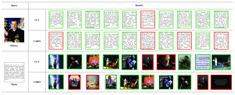
Figure 5: Examples of the bi-modal retrieval results with hand-crafted feature on Wikipedia dataset by our CCL approach and CMDN [11]. It should be noted that, in these examples, the correct retrieval results are with green borders, while the wrong results are with red borders.

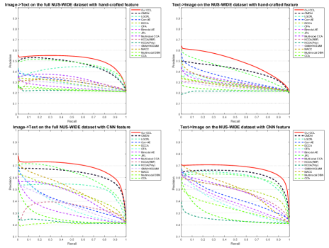
Figure 6: Precision-Recall curves of bi-modal retrieval on NUS-WIDE dataset.

IV-F Comparison with State-of-the-art Methods

This part presents the experimental results and analyses on our CCL approach as well as all the compared methods. As shown in Tables I and II, our approach achieves the best results in both bi-modal and all-modal retrieval tasks on Wikipedia dataset with both hand-crafted feature and CNN feature. Some retrieval results are shown by our CCL approach and CMDN in Figure 5, from which we can see that our proposed CCL approach can effectively reduce the failure cases compared with other methods. And a few categories in this dataset are difficult to be distinguished due to the high-level semantics such as “history” category, which leads to confusions during retrieval process on both our CCL approach and the compared methods. But our approach still achieves the best retrieval accuracy with the least failure cases. Besides, we have made classification on the failure cases with the following two types: (1) Failure due to the confusion in the image instance, which indicates that small variance between the image instances of different categories leads to wrong retrieval results; (2) Failure due to the confusion in the text instance, which is similarly caused by small variance between the text instances of different categories.

Besides, the results on other 5 datasets with both hand-crafted feature and CNN feature are shown from Tables III to XII. The trends of the results on these datasets are similar to Wikipedia dataset and our CCL approach keeps the best. Also we can observe that the compared methods generally benefit greatly from CNN feature and achieve accuracy improvement. Our CCL approach can stably benefit from CNN image feature and keeps the best among all compared methods. Figures 6 and 7 show the precision-recall curves and precision-scope curves of bi-modal retrieval task on NUS-WIDE dataset, which can further verify the effectiveness of our CCL approach.

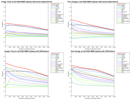
Figure 7: Precision-Scope curves of bi-modal retrieval on NUS-WIDE dataset.

As shown from Tables I to XII, our CCL approach keeps advantage with all 13 compared methods on 6 datasets, and the results show similar trends. Among the traditional methods, CFA minimizes the Frobenius norm in transformed domain, KCCA adopts kernel functions, and multi-label CCA considers the high-level semantic information, which makes them perform better than classical baseline CCA. It should be noted that KCCA has lower accuracy than CFA in some settings for the fact that KCCA can only learn a coarse association between different modalities. In addition, the performance of different kernel functions may vary greatly. Especially, Poly kernel has lower accuracy than Gaussian kernel on most settings because it cannot effectively handle the large-scale training data. MACC further embeds the projections into a local context based on KCCA. JRL outperforms the above methods by using semi-supervised regularization and sparse regularization. GMM+HGLMM and LGCFL achieve the best accuracies among the traditional methods in most cases, because GMM+HGLMM combines different kinds of Mixture Models to improve sentence representation, while LGCFL jointly learns basis matrices using a local group based priori. As for the DNN-based methods, Multimodal DBN has the worst accuracy among them. It is because only a joint distribution is learned on the top of two-layer DBN for each modality, which focuses more on learning the complementarity between different modalities rather than the correlation across them. Bimodal AE and Corr-AE have better accuracies because they jointly consider the reconstruction information. DCCA extends traditional CCA by maximizing the correlation between two separate networks. Our previous work CMDN achieves the best accuracy among the DNN-based methods because of jointly modeling on intra-modality and inter-modality correlation in both two learning stages. It should be noted that our proposed CCL approach achieves the best accuracy compared with state-of-the-art methods for the following 3 aspects: (1) The multi-grained fusion on both coarse-grained instances and fine-grained patches, while the compared methods only use the original modality instances. (2) The multi-task learning strategy to adaptively balance intra-modality semantic category constraints and inter-modality pairwise similarity constraints, while the compared methods only adopt single-loss regularization failing to effectively exploit and balance the above constraints. (3) Jointly optimizing on the intrinsic intra-modality and inter-modality correlation, while the compared methods ignore the inter-modality correlation in the separate representation learning for the first stage.

IV-G Experimental Analysis

IV-G1 Network and Parameter Analysis

For the convergence experiments, which are conducted on Wikipedia and NUS-WIDE datasets as examples due to the page limitation, we show the curves of downtrend on the loss value in Figure 8 to verify the convergence of our proposed approach. We can see that our CCL approach can converge quickly within 2K iterations, which shows its efficiency. For the training details of the network, we conduct the experiments on the effect of some key parameters also on Wikipedia and NUS-WIDE datasets, including learning rate ranging from 1e-2 to 1e-6, and the margin parameter $\alpha$ in the loss function in Eq.(11) ranging from 0.5 to 2.5. The results are shown in Figure 9. And we can see that our CCL approach gets the best performance at the learning rate of 1e-3 on Wikipedia dataset and 1e-5 on NUS-WIDE dataset, while the results change little from 1e-3 to 1e-6. Besides, the performance is insensitive to the value change of margin parameter.

For the parameter size, we conduct experiments between our proposed approach and two best DNN-based methods namely CMDN and Corr-AE with the comparable sizes of parameter space on Wikipedia dataset taking CNN feature as input. Specifically, our CCL approach originally has about 21K parameters, while the CMDN and Corr-AE have about 17K and 10K parameters respectively. So we decrease the size of parameter space of CCL and CMDN, by reducing the number of layers and the number of hidden units on each layer to achieve the comparable parameter size with Corr-AE with about 10K parameters, which is called CCL-small and CMDN-small in Table XIII. The experimental results are shown in Table XIII. We can see that CCL-small still outperforms CMDN-small and Corr-AE with comparable parameter sizes. It shows that although retrieval accuracy can be improved by increasing parameter size, the size of parameter space is not the key point for the improvement. The effective modeling of intra-modality and inter-modality correlation makes great contribution to the final performance.

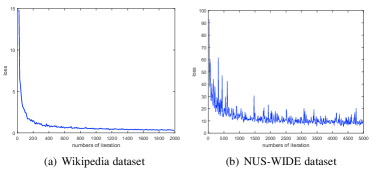
Figure 8: Convergence experiments of our proposed CCL approach conducted on Wikipedia dataset and NUS-WIDE dataset, which show the curves of downtrend on the loss value.

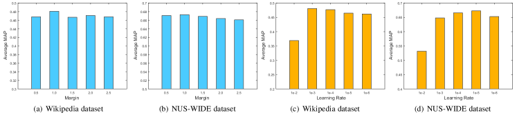
Figure 9: Experiments on the training detail of our proposed CCL approach, including learning rate and the margin parameter $\alpha$, on Wikipedia dataset and NUS-WIDE dataset. It should be noted that we report the average MAP score of Image$\rightarrow$Text and Text$\rightarrow$Image tasks.

TABLE XIII: Experiments on the parameter size between representative DNN-based methods.

Dataset	Method	MAP with CNN feature
		Image$\rightarrow$Text	Text$\rightarrow$Image	Average
Wikipedia dataset	CCL	0.504	0.457	0.481
	CCL-small	0.490	0.444	0.467
	CMDN-small	0.463	0.408	0.436
	Corr-AE	0.402	0.395	0.399

TABLE XIV: Training and testing time for our CCL approach and compared methods.

Method	Training		Testing
	Wikipedia	NUS-WIDE	Wikipedia	NUS-WIDE
Our CCL Approach	2794s	2958s	0.40s	281s
CMDN [11]	2102s	2434s	0.38s	275s
DCCA [12]	683s	1636s	0.42s	289s
Corr-AE [10]	1051s	1237s	0.37s	283s
Multimodal DBN [13]	1343s	1523s	0.39s	275s
Bimodal AE [15]	974s	1304s	0.35s	279s
JRL [8]	211s	1426s	0.26s	75s
GMM+HGLMM [19]	235s	803s	0.30s	143s
Multi-label CCA [22]	56s	3924s	0.29s	110s
MACC [23]	62s	2340s	0.28s	283s
KCCA(Gaussian) [17]	35s	2018s	0.35s	2183s
KCCA(Poly) [17]	27s	2228s	0.31s	2179s
LGCFL [40]	8.2s	28s	0.26s	65s
CFA [21]	7.5s	8.7s	0.76s	264s
CCA [16]	0.3s	1.4s	0.28s	108s

TABLE XV: Baseline experiments on Bi-modal Retrieval, where CCL (only coarse-grained) means CCL with only the original instances as input, while CCL (only fine-grained) means CCL with only the patches of original instance as input. And CCL (only intra-modality) means CCL with only intra-modality separate representation learning, while CCL (only inter-modality) means CCL with only inter-modality separate representation learning.

Dataset	Method	MAP with hand-crafted feature			MAP with CNN feature
		Image$\rightarrow$Text	Text$\rightarrow$Image	Average	Image$\rightarrow$Text	Text$\rightarrow$Image	Average
Wikipedia dataset	Our CCL Approach	0.418	0.359	0.389	0.504	0.457	0.481
	CCL (only coarse-grained)	0.399	0.329	0.364	0.457	0.429	0.443
	CCL (only fine-grained)	0.393	0.328	0.361	0.456	0.400	0.428
	CCL (only intra-modality)	0.384	0.332	0.358	0.483	0.444	0.464
	CCL (only inter-modality)	0.380	0.321	0.351	0.471	0.395	0.433
NUS-WIDE-10K dataset	Our CCL Approach	0.400	0.401	0.401	0.506	0.535	0.521
	CCL (only coarse-grained)	0.371	0.356	0.364	0.483	0.516	0.500
	CCL (only fine-grained)	0.368	0.358	0.363	0.414	0.436	0.425
	CCL (only intra-modality)	0.377	0.374	0.376	0.488	0.520	0.504
	CCL (only inter-modality)	0.347	0.346	0.347	0.442	0.470	0.456
Pascal Sentence dataset	Our CCL Approach	0.359	0.346	0.353	0.566	0.560	0.563
	CCL (only coarse-grained)	0.283	0.286	0.285	0.514	0.508	0.511
	CCL (only fine-grained)	0.255	0.239	0.247	0.386	0.393	0.390
	CCL (only intra-modality)	0.296	0.272	0.284	0.521	0.520	0.521
	CCL (only inter-modality)	0.217	0.217	0.217	0.420	0.383	0.402
NUS-WIDE dataset	Our CCL Approach	0.513	0.489	0.501	0.671	0.676	0.674
	CCL (only coarse-grained)	0.502	0.466	0.484	0.665	0.670	0.668
	CCL (only fine-grained)	0.485	0.451	0.468	0.595	0.604	0.600
	CCL (only intra-modality)	0.487	0.460	0.474	0.652	0.660	0.656
	CCL (only inter-modality)	0.427	0.400	0.414	0.515	0.519	0.517

TABLE XVI: Baseline experiments of Image Annotation on Flickr-30K and MS-COCO datasets.

Dataset	Method	Hand-crafted feature			CNN feature
		R@1	R@5	R@10	R@1	R@5	R@10
Flickr-30K dataset	Our CCL Approach	0.088	0.276	0.393	0.377	0.694	0.811
	CCL (only coarse-grained)	0.059	0.192	0.294	0.286	0.587	0.719
	CCL (only fine-grained)	0.021	0.100	0.171	0.170	0.436	0.581
	CCL (only intra-modality)	0.040	0.133	0.220	0.312	0.641	0.753
	CCL (only inter-modality)	0.029	0.125	0.212	0.232	0.544	0.694
MS-COCO dataset	Our CCL Approach	0.063	0.196	0.298	0.186	0.474	0.625
	CCL (only coarse-grained)	0.048	0.154	0.241	0.127	0.364	0.510
	CCL (only fine-grained)	0.030	0.100	0.162	0.102	0.304	0.436
	CCL (only intra-modality)	0.058	0.177	0.264	0.147	0.406	0.556
	CCL (only inter-modality)	0.026	0.096	0.160	0.121	0.340	0.485

TABLE XVII: Baseline experiments of Image Retrieval on Flickr-30K and MS-COCO datasets.

Dataset	Method	Hand-crafted feature			CNN feature
		R@1	R@5	R@10	R@1	R@5	R@10
Flickr-30K dataset	Our CCL Approach	0.090	0.253	0.361	0.373	0.684	0.800
	CCL (only coarse-grained)	0.054	0.179	0.272	0.255	0.567	0.692
	CCL (only fine-grained)	0.021	0.098	0.172	0.172	0.422	0.569
	CCL (only intra-modality)	0.033	0.135	0.205	0.310	0.613	0.745
	CCL (only inter-modality)	0.028	0.116	0.205	0.228	0.544	0.688
MS-COCO dataset	Our CCL Approach	0.064	0.197	0.296	0.196	0.469	0.623
	CCL (only coarse-grained)	0.047	0.162	0.247	0.132	0.358	0.505
	CCL (only fine-grained)	0.027	0.100	0.160	0.107	0.299	0.430
	CCL (only intra-modality)	0.056	0.181	0.273	0.150	0.402	0.547
	CCL (only inter-modality)	0.026	0.104	0.171	0.119	0.330	0.473

IV-G2 Execution Time

We measure the execution time for our proposed CCL approach as well as all the compared methods. It should be noted that we measure the training and testing time for different methods without the time for data preprocessing such as feature extraction and patch segmentation. Besides, we adopt small-scale Wikipedia dataset and large-scale NUS-WIDE dataset, and use CNN feature as input. The execution time is recorded on a PC with i7-5930K CPU @ 3.50GHz, 64GB memory and one GPU of NVIDIA Titan X with 12GB memory. The training time is shown in Table XIV. We can see that the training time of all methods increases with the number of training instances increasing, especially for some traditional methods such as JRL and KCCA due to the large amount of calculation on matrix multiplication. Besides, among the DNN-based methods, the training time of Bimodal AE, Multimodal DBN and Corr-AE is close to each other and less than our proposed CCL approach and CMDN. It is because our CCL approach and CMDN have more components to train for different purposes, such as different subnetworks for coarse-grained and fine-grained representation learning and the multi-grained fusion subnetwork in CCL approach, while the compared DNN-based methods ignore the complementary fine-grained clues provided by their patches. On testing time, all the methods including our proposed CCL approach have almost the same testing time on small-scale Wikipedia dataset. While on large-scale NUS-WIDE dataset, the time has some difference mainly because the dimensional numbers of common representation generated from different methods vary greatly, which leads to different costs in distance measurement with the increasing number of testing instances. For example, KCCA has the longest testing time due to its high-dimensional common representation with about 10,000 dimensions, which is much higher than other compared methods having less than 1,024 dimensions. From the above results, we can see that the training stage is the key point for our proposed CCL approach to achieve the best accuracy, while it costs little extra time in the testing stage.

IV-G3 Baseline Experiments

Tables XV to XVII show the accuracies of our CCL approach and the baseline approaches. CCL (only coarse-grained) means only the coarse-grained original instances are used to generate common representation, while CCL (only fine-grained) means only the fine-grained patches are adopted. Due to only the coarse-grained or fine-grained information is adopted, we drop the joint RBM which is used to fuse multi-grained representation, and the other parts of the network keep exactly the same in our CCL approach for fair comparison. The coarse-grained and fine-grained information can be effectively integrated by CCL approach to make cross-modal correlation more precise, which leads to better accuracy than CCL (only coarse-grained) and CCL (only fine-grained) that use single-grained information merely.

Besides, we also show the baseline experiments to verify the effectiveness of combination of intra-modality and inter-modality correlation in the first learning stage. CCL (only intra-modality) means CCL with only intra-modality reconstruction learning error $L_{r}$ in Eq.(11), while CCL (only inter-modality) means CCL with only inter-modality correlation learning error $L_{c}$ in Eq.(11) for separate representation learning. We can see that learning intra-modality and inter-modality correlation simultaneously by joint optimization achieves higher MAP score than learning only one of them, which indicates the complementarity of the two kinds of information, and it can be effectively exploited by our CCL approach to achieve better accuracy.

The above baseline experimental results verify the contribution of each component in our CCL approach. First, inter-modality correlation can provide rich complementary context to intra-modality correlation for learning better separate representation, which can capture the important hints to boost common representation learning. Second, fusion of complementary coarse-grained instances and fine-grained patches can lead to more accurate cross-modal common representation.

V Conclusion

In this paper, a cross-modal correlation learning approach has been proposed with multi-grained fusion by hierarchical network. In the first learning stage, separate representation is learned by jointly optimizing intra-modality and inter-modality correlation, which can effectively capture the intrinsic correlation and rich complementary information in different modalities. In the second learning stage, a multi-task learning strategy, which adaptively balances intra-modality semantic category constraints and inter-modality pairwise similarity constraints, is adopted to fully exploit the intrinsic relevance between them. Besides, the coarse-grained instances and fine-grained patches are integrated to make cross-modal correlation more precise. Comprehensive experimental results show effectiveness of our CCL approach compared with 13 state-of-the-art methods on 6 widely-used cross-modal datasets.

The future work lies in two aspects: First, we will focus on learning better fine-grained representation with more effective and precise segmentation methods. Second, we will attempt to apply semi-supervised regularization into our framework to make full use of the unlabeled data. Both of them will be employed to further boost the cross-modal retrieval accuracy.

Yuxin Peng is the professor of Institute of Computer Science and Technology (ICST), Peking University, and the chief scientist of 863 Program (National Hi-Tech Research and Development Program of China). He received the Ph.D. degree in computer application technology from Peking University in Jul. 2003. After that, he worked as an assistant professor in ICST, Peking University. He was promoted to associate professor and professor in Peking University in Aug. 2005 and Aug. 2010 respectively. In 2006, he was authorized by the “Program for New Star in Science and Technology of Beijing” and the “Program for New Century Excellent Talents in University (NCET)”. He has published over 100 papers in refereed international journals and conference proceedings, including IJCV, TIP, TCSVT, TMM, PR, ACM MM, ICCV, CVPR, IJCAI, AAAI, etc. He led his team to participate in TRECVID (TREC Video Retrieval Evaluation) many times. In TRECVID 2009, his team won four first places on 4 sub-tasks of the High-Level Feature Extraction (HLFE) task and Search task. In TRECVID 2012, his team gained four first places on all 4 sub-tasks of the Instance Search (INS) task and Known-Item Search (KIS) task. In TRECVID 2014, his team gained the first place in the Interactive Instance Search task. His team also gained both two first places in the INS task of TRECVID 2015 and 2016. Besides, he won the first prize of Beijing Science and Technology Award for Technological Invention in 2016 (ranking first). He has applied 34 patents, and obtained 16 of them. His current research interests mainly include cross-media analysis and reasoning, image and video analysis and retrieval, and computer vision.

Jinwei Qi received the B.S. degree in computer science and technology from Peking University, in Jul. 2016. He is currently pursuing the M.S. degree with the Institute of Computer Science and Technology (ICST), Peking University. His current research interests include cross-media retrieval and deep learning.

Xin Huang received the B.S. degree in computer science and technology from Peking University, in Jul. 2014. He is currently pursuing the Ph.D. degree in the Institute of Computer Science and Technology (ICST), Peking University. His research interests include cross-media reasoning and deep learning.

Yuxin Yuan received the B.S. degree in electronic science and engineering from Nanjing University, in Jul. 2015. He is currently pursuing the M.S. degree in the Institute of Computer Science and Technology (ICST), Peking University. His current research interests include cross-media retrieval and deep learning.

References

- [1] Y. Hu, X. Cheng, L.-T. Chia, X. Xie, D. Rajan, and A.-H. Tan, “Coherent phrase model for efficient image near-duplicate retrieval,” IEEE Transactions on Multimedia (TMM), vol. 11, no. 8, pp. 1434–1445, 2009.
- [2] Y. Peng and C.-W. Ngo, “Clip-based similarity measure for query-dependent clip retrieval and video summarization,” IEEE Transactions on Circuits and Systems for Video Technology (TCSVT), vol. 16, no. 5, pp. 612–627, 2006.
- [3] A. Znaidia, A. Shabou, H. Le Borgne, C. Hudelot, and N. Paragios, “Bag-of-multimedia-words for image classification,” in International Conference on Pattern Recognition (ICPR), 2012, pp. 1509–1512.
- [4] Y. Liu, W.-L. Zhao, C.-W. Ngo, C.-S. Xu, and H.-Q. Lu, “Coherent bag-of audio words model for efficient large-scale video copy detection,” in ACM International Conference on Image and Video Retrieval (CIVR), 2010, pp. 89–96.
- [5] N. Rasiwasia, J. Costa Pereira, E. Coviello, G. Doyle, G. R. Lanckriet, R. Levy, and N. Vasconcelos, “A new approach to cross-modal multimedia retrieval,” in ACM International Conference on Multimedia (ACM-MM), 2010, pp. 251–260.
- [6] P. Daras, S. Manolopoulou, and A. Axenopoulos, “Search and retrieval of rich media objects supporting multiple multimodal queries,” IEEE Transactions on Multimedia (TMM), vol. 14, no. 3, pp. 734–746, 2012.
- [7] L. Zhang, B. Ma, G. Li, Q. Huang, and Q. Tian, “Cross-modal retrieval using multi-ordered discriminative structured subspace learning,” IEEE Transactions on Multimedia (TMM), vol. 19, no. 6, pp. 1220–1233, 2017.
- [8] X. Zhai, Y. Peng, and J. Xiao, “Learning cross-media joint representation with sparse and semi-supervised regularization,” IEEE Transactions on Circuits and Systems for Video Technology (TCSVT), vol. 24, pp. 965–978, 2014.
- [9] G. Andrew, R. Arora, J. A. Bilmes, and K. Livescu, “Deep canonical correlation analysis,” in International Conference on Machine Learning (ICML), 2013, pp. 1247–1255.
- [10] F. Feng, X. Wang, and R. Li, “Cross-modal retrieval with correspondence autoencoder,” in ACM International Conference on Multimedia (ACM-MM), 2014, pp. 7–16.
- [11] Y. Peng, X. Huang, and J. Qi, “Cross-media shared representation by hierarchical learning with multiple deep networks,” in International Joint Conference on Artificial Intelligence (IJCAI), 2016, pp. 3846–3853.
- [12] F. Yan and K. Mikolajczyk, “Deep correlation for matching images and text,” in Conference on Computer Vision and Pattern Recognition (CVPR), 2015, pp. 3441–3450.
- [13] N. Srivastava and R. Salakhutdinov, “Learning representations for multimodal data with deep belief nets,” in International Conference on Machine Learning (ICML) Workshop, 2012.
- [14] X. He and Y. Peng, “Weakly supervised learning of part selection model with spatial constraints for fine-grained image classification,” in AAAI Conference on Artificial Intelligence (AAAI), 2017, pp. 4075–4081.
- [15] J. Ngiam, A. Khosla, M. Kim, J. Nam, H. Lee, and A. Y. Ng, “Multimodal deep learning,” in International Conference on Machine Learning (ICML), 2011, pp. 689–696.
- [16] H. Hotelling, “Relations between two sets of variates,” Biometrika, pp. 321–377, 1936.
- [17] D. R. Hardoon, S. Szedmák, and J. Shawe-Taylor, “Canonical correlation analysis: An overview with application to learning methods,” Neural Computation, vol. 16, no. 12, pp. 2639–2664, 2004.
- [18] H. Bredin and G. Chollet, “Audio-visual speech synchrony measure for talking-face identity verification,” in International Conference on Acoustics, Speech and Signal Processing (ICASSP), vol. 2, 2007, pp. 233–236.
- [19] B. Klein, G. Lev, G. Sadeh, and L. Wolf, “Associating neural word embeddings with deep image representations using fisher vectors,” in Conference on Computer Vision and Pattern Recognition (CVPR), 2015, pp. 4437–4446.
- [20] Y. Gong, Q. Ke, M. Isard, and S. Lazebnik, “A multi-view embedding space for modeling internet images, tags, and their semantics,” International Journal of Computer Vision (IJCV), vol. 106, no. 2, pp. 210–233, 2014.
- [21] D. Li, N. Dimitrova, M. Li, and I. K. Sethi, “Multimedia content processing through cross-modal association,” in ACM International Conference on Multimedia (ACM-MM), 2003, pp. 604–611.
- [22] V. Ranjan, N. Rasiwasia, and C. V. Jawahar, “Multi-label cross-modal retrieval,” in IEEE International Conference on Computer Vision (ICCV), 2015, pp. 4094–4102.
- [23] T. Q. N. Tran, H. L. Borgne, and M. Crucianu, “Aggregating image and text quantized correlated components,” in Conference on Computer Vision and Pattern Recognition (CVPR), 2016, pp. 2046–2054.
- [24] Y. Hua, S. Wang, S. Liu, A. Cai, and Q. Huang, “Cross-modal correlation learning by adaptive hierarchical semantic aggregation,” IEEE Transactions on Multimedia (TMM), vol. 18, no. 6, pp. 1201–1216, 2016.
- [25] X. Zhai, Y. Peng, and J. Xiao, “Heterogeneous metric learning with joint graph regularization for cross-media retrieval,” in AAAI Conference on Artificial Intelligence (AAAI), 2013.
- [26] K. Wang, R. He, L. Wang, W. Wang, and T. Tan, “Joint feature selection and subspace learning for cross-modal retrieval,” IEEE Transactions on Pattern Analysis and Machine Intelligence (TPAMI), vol. 38, no. 10, pp. 2010–2023, 2016.
- [27] K. He, X. Zhang, S. Ren, and J. Sun, “Deep residual learning for image recognition,” in Conference on Computer Vision and Pattern Recognition (CVPR), 2016, pp. 770–778.
- [28] J. Dai, Y. Li, K. He, and J. Sun, “R-FCN: object detection via region-based fully convolutional networks,” in Conference on Neural Information Processing Systems (NIPS), 2016, pp. 379–387.
- [29] A. Krizhevsky, I. Sutskever, and G. E. Hinton, “Imagenet classification with deep convolutional neural networks,” in Conference on Neural Information Processing Systems (NIPS), 2012, pp. 1106–1114.
- [30] Z. Wu, Y. Jiang, X. Wang, H. Ye, and X. Xue, “Multi-stream multi-class fusion of deep networks for video classification,” in ACM International Conference on Multimedia (ACM-MM), 2016, pp. 791–800.
- [31] R. Salakhutdinov and G. E. Hinton, “Replicated softmax: an undirected topic model,” in Conference on Neural Information Processing Systems (NIPS), 2009, pp. 1607–1614.
- [32] P. Vincent, H. Larochelle, Y. Bengio, and P. Manzagol, “Extracting and composing robust features with denoising autoencoders,” in International Conference on Machine Learning (ICML), 2008, pp. 1096–1103.
- [33] Y. Sun, X. Wang, and X. Tang, “Deep learning face representation by joint identification-verification,” in Conference on Neural Information Processing Systems (NIPS), 2014, pp. 1988–1996.
- [34] S. Ren, K. He, R. B. Girshick, and J. Sun, “Faster R-CNN: towards real-time object detection with region proposal networks,” in Conference on Neural Information Processing Systems (NIPS), 2015, pp. 91–99.
- [35] A. H. Abdulnabi, G. Wang, J. Lu, and K. Jia, “Multi-task CNN model for attribute prediction,” IEEE Transactions on Multimedia (TMM), vol. 17, no. 11, pp. 1949–1959, 2015.
- [36] Y. Peng, X. Zhai, Y. Zhao, and X. Huang, “Semi-supervised cross-media feature learning with unified patch graph regularization,” IEEE Transactions on Circuits and Systems for Video Technology (TCSVT), vol. 26, no. 3, pp. 583–596, 2016.
- [37] G. E. Hinton, S. Osindero, and Y. W. Teh, “A fast learning algorithm for deep belief nets,” Neural Computation, vol. 18, no. 7, pp. 1527–1554, 2006.
- [38] M. Welling, M. Rosen-Zvi, and G. E. Hinton, “Exponential family harmoniums with an application to information retrieval,” in Conference on Neural Information Processing Systems (NIPS), 2004, pp. 1481–1488.
- [39] J. R. R. Uijlings, K. E. A. van de Sande, T. Gevers, and A. W. M. Smeulders, “Selective search for object recognition,” International Journal of Computer Vision (IJCV), vol. 104, no. 2, pp. 154–171, 2013.
- [40] C. Kang, S. Xiang, S. Liao, C. Xu, and C. Pan, “Learning consistent feature representation for cross-modal multimedia retrieval,” IEEE Transactions on Multimedia (TMM), vol. 17, no. 3, pp. 370–381, 2015.
- [41] T. Chua, J. Tang, R. Hong, H. Li, Z. Luo, and Y. Zheng, “Nus-wide: a real-world web image database from national university of singapore,” in ACM International Conference on Image and Video Retrieval (CIVR), 2009, pp. 1–9.
- [42] Y. Zhuang, Y. Wang, F. Wu, Y. Zhang, and W. Lu, “Supervised coupled dictionary learning with group structures for multi-modal retrieval,” in AAAI Conference on Artificial Intelligence (AAAI), 2013, pp. 1070–1076.
- [43] C. Rashtchian, P. Young, M. Hodosh, and J. Hockenmaier, “Collecting image annotations using amazon’s mechanical turk,” in NAACL HLT 2010 Workshop on Creating Speech and Language Data with Amazon’s Mechanical Turk, 2010, pp. 139–147.
- [44] P. Young, A. Lai, M. Hodosh, and J. Hockenmaier, “From image descriptions to visual denotations: New similarity metrics for semantic inference over event descriptions,” Transactions of the Association for Computational Linguistics (TACL), vol. 2, pp. 67–78, 2014.
- [45] T. Lin, M. Maire, S. J. Belongie, J. Hays, P. Perona, D. Ramanan, P. Dollár, and C. L. Zitnick, “Microsoft coco: Common objects in context,” in European Conference on Computer Vision (ECCV), 2014, pp. 740–755.
- [46] M. Simon, E. Rodner, and J. Denzler, “Imagenet pre-trained models with batch normalization,” arXiv preprint arXiv:1612.01452, 2016.
- [47] Y. Jia, E. Shelhamer, J. Donahue, S. Karayev, J. Long, R. Girshick, S. Guadarrama, and T. Darrell, “Caffe: Convolutional architecture for fast feature embedding,” arXiv preprint arXiv:1408.5093, 2014.
- [48] G. E. Hinton, N. Srivastava, A. Krizhevsky, I. Sutskever, and R. Salakhutdinov, “Improving neural networks by preventing co-adaptation of feature detectors,” arXiv preprint arXiv:1207.0580, 2012.