Effect of long-range structural corrugations on magnetotransport properties of phosphorene in tilted magnetic field

Abstract

Rippling is an inherent quality of two-dimensional materials playing an important role in determining their properties. Here, we study the effect of structural corrugations on the electronic and transport properties of monolayer black phosphorus (phosphorene) in the presence of tilted magnetic field. We follow a perturbative approach to obtain analytical corrections to the spectrum of Landau levels induced by a long-wavelength corrugation potential. We show that surface corrugations have a non-negligible effect on the electronic spectrum of phosphorene in tilted magnetic field. Particularly, the Landau levels are shown to exhibit deviations from the linear field dependence. The observed effect become especially pronounced at large tilt angles and corrugation amplitudes. Magnetotransport properties are further examined in the low temperature regime taking into account impurity scattering. We calculate magnetic field dependence of the longitudinal and Hall resistivities and find that the nonlinear effects reflecting the corrugation might be observed even in moderate fields ($B<10$ T).

I Introduction

After the first synthesis of graphene Novoselov et al. (2004), the interest in two-dimensional (2D) materials has grown considerably over the past decade. The gapless energy spectrum of graphene has stimulated the search for 2D semiconductors, more suitable for traditional electronic and optoelectronic applications. Besides the other group IV materials Vogt et al. (2012); Dávila et al. (2014); Bampoulis et al. (2014); Zhang et al. (2016); Zhu et al. (2015) and a variety of transition-metal dichalcogenidesWang et al. (2012); Jariwala et al. (2014) fabricated in recent years, new elemental materials appear in the focus of attention. In this context, few-layer black phosphorus is one of the most promising 2D materials potentially interesting for practical applications Ling et al. (2015); Castellanos-Gomez (2015); Carvalho et al. (2016) because of its relatively high carrier mobilityKoenig et al. (2014); Liu et al. (2014); Li et al. (2014), tunable energy gap of 0.3–2.0 eV Tran et al. (2014); Rudenko et al. (2015); Qiao et al. (2014), and intrinsic anisotropy Qiao et al. (2014); Xia et al. (2014); Wang et al. (2015) resulting in, for instance, unusual optical response Low et al. (2014); Nemilentsau et al. (2016). Compared to graphene, properties of black phosphorus are considerably less studied theoretically, which hinders the understanding of experimentally observable phenomena.

2D materials are known to be intrinsically unstable with respect to long-wavelength thermal fluctuations, resulting in the formation of a corrugated or rippled structure in accordance with the Mermin-Wagner theorem Mermin (1968). Earlier studies demonstrated that rippling is an intrinsic feature of graphene, which affects its electronic properties Meyer et al. (2007); Fasolino et al. (2007); de Juan et al. (2007); Isacsson et al. (2008); Guinea et al. (2008a, b); Cortijo and Vozmediano (2009); Costamagna et al. (2010). Other 2D structures were also shown to have a tendency to form ripples, such as, for example, in hexagonal boron nitride Meyer et al. (2009), transition metal dichalcogenides Brivio et al. (2011); Miro et al. (2013), and black phosphorus Kou et al. (2015); Zhou et al. (2016); Wang et al. (2016). Although 2D materials are usually deposited on substrates, which may suppress the formation of intrinsic rippling, surface roughness of common dielectrics like SiO₂ represents by itself another source of structural corrugations Ishigami et al. (2007); Geringer et al. (2009); Lui et al. (2009).

Understanding the dynamics of charge carriers in 2D materials under realistic conditions is a problem of practical importance as it determines observable transport properties. Magnetotransport measurements offer a powerful tool to probe carrier dynamics at the quantum level. Recently, several studies have reported quantum transport measurements in few-layer black phosphorus Chen et al. (2015); Li et al. (2015); Tayari et al. (2015); Gillgren et al. (2015); Li et al. (2016); Long et al. (2016); Tran et al. (2017); Long et al. (2017). Interpretation of experimental observations is usually carried out on a phenomenological level without explicit consideration of their microscopic nature. On the other hand, theoretical description of quantum transport at the level of model HamiltoniansYuan et al. (2015); Zhou et al. (2015a); Tahir et al. (2015); Jiang et al. (2015); Zhou et al. (2015b); Yuan et al. (2016) has limited capability to capture essential environmental effects caused by impurities, substrates, and structural corrugations. The role of those effects in magnetotransport properties of few-layer black phosphorus is not well understood.

In this paper, we study the role of long-range structural corrugations on the Landau levels (LLs) and magnetotransport properties of monolayer black phosphorus (MBP) in the presence of a tilted magnetic field. We use a perturbative approach to obtain first-order corrections to the energy spectrum induced by a corrugation potential. We find noticeable deviations of LLs from the linear dependence on magnetic field, which are also apparent in the calculated longitudinal and Hall resistivities at not very strong fields.

The paper is organized as follows. The theory part is presented in Sec. II, where we first consider unperturbed Hamiltonian for MBP in perpendicular magnetic field (Sec. II A), and then obtain a correction to the Hamiltonian in the presence of a corrugation potential in tilted magnetic field (Sec. II B). In Sec. II C, we present the formalism of the linear response theory, which is used to calculate magnetotransport properties of MBP. The results and their discussion are presented in Sec. III. In Sec. IV, we briefly summarize our results and conclude the paper.

II Theory

II.1 Pristine MBP in perpendicular magnetic field

The energy spectrum of MBP can be described by a four-band tight-binding model Rudenko and Katsnelson (2014). However, $C_{2h}$ group invariance of the MBP lattice enables one to describe the system by a two-band model Rodin et al. (2014). An effective continuum model can be obtained by expanding the tight-binding Hamiltonian around the $\mathrm{\Gamma}$ point, yielding a good agreement with the tight-binding results in the energy range of $\sim$3.5 eV Ezawa (2014); Pereira and Katsnelson (2015). In the long-wavelength limit, the continuum Hamiltonian of MBP can be written as Pereira and Katsnelson (2015),

$$\mathcal{H}_{0}=\left[\begin{array}[]{cc}u_{0}+\bar{\eta}_{x}\pi_{x}^{2}+\bar{\eta}_{y}\pi_{y}^{2}&\delta+\bar{\gamma}_{x}\pi_{x}^{2}+\bar{\gamma}_{y}\pi_{y}^{2}+i\bar{\chi}\pi_{y}\\ \delta+\bar{\gamma}_{x}\pi_{x}^{2}+\bar{\gamma}_{y}\pi_{y}^{2}-i\bar{\chi}\pi_{y}&u_{0}+\bar{\eta}_{x}\pi_{x}^{2}+\bar{\eta}_{y}\pi_{y}^{2}\end{array}\right].$$ (1)

Eq. (1) can be divided into quadratic and linear terms, respectively, as

$$\mathcal{H}_{0}^{\mathrm{quad}}=\left[\begin{array}[]{cc}u_{0}+\bar{\eta}_{x}\pi_{x}^{2}+\bar{\eta}_{y}\pi_{y}^{2}&\bar{\gamma}_{x}\pi_{x}^{2}+\bar{\gamma}_{y}\pi_{y}^{2}\\ \bar{\gamma}_{x}\pi_{x}^{2}+\bar{\gamma}_{y}\pi_{y}^{2}&u_{0}+\bar{\eta}_{x}\pi_{x}^{2}+\bar{\eta}_{y}\pi_{y}^{2}\end{array}\right],$$ (2)

$$\mathcal{H}_{0}^{\mathrm{lin}}=\left[\begin{array}[]{cc}0&\delta+i\bar{\chi}\pi_{y}\\ \delta-i\bar{\chi}\pi_{y}&0\end{array}\right].$$ (3)

Here, $\bar{\eta}_{i}=\eta_{i}/\hbar^{2}$ ($\eta_{x}=0.58$ eVŲ and $\eta_{y}=1.01$ eVŲ), $\bar{\gamma}_{i}=\gamma_{i}/\hbar^{2}$ ($\gamma_{x}=3.93$ eVŲ and $\gamma_{y}=3.83$ eVŲ), $\bar{\chi}=\chi/\hbar$ ($\chi=5.25$ eVÅ), $u_{0}=-0.42$ eV and $\delta=0.76$ eV Pereira and Katsnelson (2015), and $\pi_{i}$ is the 2D canonical momentum. If magnetic field is applied normal to the MBP plane, B=(0,0,B), in symmetric gauge $\pi_{x}=p_{x}-(eB/2)y$ and $\pi_{y}=p_{y}+(eB/2)x$, where $p_{i}$ is the momentum operator. One can express $p_{i}$ and $r_{i}$ in terms of the creation $b_{i}^{{\dagger}}$ and annihilation $b_{i}$ operators as

$$p_{i} = \left(\frac{m^{\lambda}_{i}\hbar\omega_{\lambda}}{2}\right)^{1/2}(b_{i}^{\dagger}+b_{i}),$$

$$r_{i} = -i\left(\frac{\hbar}{2m^{\lambda}_{i}\omega_{\lambda}}\right)^{1/2}(b_{i}^{\dagger}-b_{i}),$$

where $\lambda$ is the band index taking $+$1 ($-$1) for the conduction (valence) band, and $i$ refers to $x$ or $y$. $\omega_{\lambda}=eB/\sqrt{m^{\lambda}_{x}m^{\lambda}_{y}}$ is the cyclotron frequency, which takes $\omega_{+}=2.668\omega_{e}$ ($\omega_{-}=2.195\omega_{e}$) for electrons (holes) with $\omega_{e}=eB/m_{0}$, and $m^{\lambda}_{i}$ are the effective masses: $m^{+}_{x}=\hbar^{2}/2(\eta_{x}+\gamma_{x})=0.846m_{0}$ and $m^{+}_{y}=\hbar^{2}/2(\eta_{y}+\gamma_{y}+\chi^{2}/2\delta)=0.166m_{0}$ for the conduction band, $m^{-}_{x}=\hbar^{2}/2(\gamma_{x}-\eta_{x})=1.140m_{0}$ and $m^{-}_{y}=\hbar^{2}/2(\eta_{y}-\gamma_{y}-\chi^{2}/2\delta)=0.182m_{0}$ for the valance band, with $m_{0}$ being the free electron mass. By diagonalizing $\mathcal{H}_{0}^{\mathrm{quad}}$, eigenvalues of the quadratic Hamiltonian become

$$E_{n}^{\mathrm{quad}} = u_{0}+(\bar{\eta}_{x}+\lambda\bar{\gamma}_{x})\left\langle n_{x}n_{y}\right|\pi_{x}^{2}\left|n_{x}n_{y}\right\rangle+(\bar{\eta}_{y}+\lambda\bar{\gamma}_{y})\left\langle n_{x}n_{y}\right|\pi_{y}^{2}\left|n_{x}n_{y}\right\rangle,$$ (4)

where

$$\left\langle n_{x}n_{y}\right|\pi_{x}^{2}\left|n_{x}n_{y}\right\rangle = \frac{m^{\lambda}_{x}\hbar\omega_{\lambda}}{2}(b_{x}^{\dagger}+b_{x})^{2}-\left(\frac{eB}{2}\right)^{2}\frac{\hbar}{2m^{\lambda}_{y}\omega_{\lambda}}(b_{y}^{\dagger}-b_{y})^{2}$$

$$- ieB\sqrt{\frac{m^{\lambda}_{x}\hbar\omega_{\lambda}}{2}}\sqrt{\frac{\hbar}{2m^{\lambda}_{y}\omega_{\lambda}}}(b_{x}^{\dagger}+b_{x})(b_{y}^{\dagger}-b_{y}),$$

$$\left\langle n_{x}n_{y}\right|\pi_{y}^{2}\left|n_{x}n_{y}\right\rangle = \frac{m^{\lambda}_{y}\hbar\omega_{\lambda}}{2}(b_{y}^{\dagger}+b_{y})^{2}-\left(\frac{eB}{2}\right)^{2}\frac{\hbar}{2m^{\lambda}_{x}\omega_{\lambda}}(b_{x}^{\dagger}-b_{x})^{2}$$ (5)

$$+ ieB\sqrt{\frac{m^{\lambda}_{y}\hbar\omega_{\lambda}}{2}}\sqrt{\frac{\hbar}{2m^{\lambda}_{x}\omega_{\lambda}}}(b_{y}^{\dagger}+b_{y})(b_{x}^{\dagger}-b_{x}).$$

In turn, diagonalization of the linear term $\mathcal{H}_{0}^{\mathrm{lin}}$ yields

$$(E_{n}^{\mathrm{lin}})^{2} = \delta^{2}+\bar{\chi}^{2}\left\langle n_{x}n_{y}\right|\pi_{y}^{2}\left|n_{x}n_{y}\right\rangle.$$ (6)

Due to the gauge independent degeneracy of LLs, we assume $n_{x}=n_{y}=n$, thus eigenvalues of the total Hamiltonian $\mathcal{H}_{0}$ can be written as (see Appendix A for more details)

$$E_{n\lambda}^{0} = E_{n}^{\mathrm{quad}}+E_{n}^{\mathrm{lin}}$$ (7)

$$= u_{0}+\lambda\left[\left|(\bar{\eta}_{x}+\lambda\bar{\gamma}_{x})\right|m^{\lambda}_{x}+\left|(\bar{\eta}_{y}+\lambda\bar{\gamma}_{y})\right|m^{\lambda}_{y}\right]\hbar\omega_{\lambda}\left(n+\frac{1}{2}\right)+\lambda\left[\delta^{2}+\bar{\chi}^{2}m^{\lambda}_{y}\hbar\omega_{\lambda}\left(n+\frac{1}{2}\right)\right]^{\frac{1}{2}}.$$

The last term can be expanded as $\delta\left[1+(\bar{\chi}^{2}m^{\lambda}_{y}/\delta^{2})\hbar\omega_{\lambda}(n+1/2)\right]^{1/2}\approx\left[\delta+(\bar{\chi}^{2}m^{\lambda}_{y}/2\delta)\hbar\omega_{\lambda}(n+1/2)\right]$. Finally, we arrive at

$$E_{n\lambda}^{0} = (u_{0}+\lambda\delta)+\lambda\hbar\omega_{\lambda}\left(n+\frac{1}{2}\right).$$ (8)

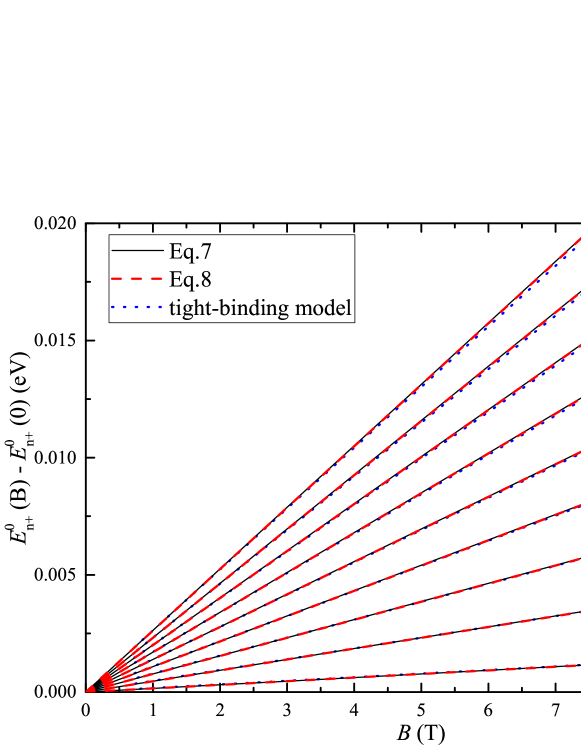
Figure 1: Landau quantization of electron states in MBP. Black line corresponds to Eq. (7), red dashed line corresponds to Eq. (8). Blue dotted line corresponds to the calculations within a tight-binding model (see Appendix B for details).

The expression given by Eq. (8) is fully consistent with the results of previous studies Pereira and Katsnelson (2015); Zhou et al. (2015a). It is clear from Fig. 1 that for $B<10$ T, two expressions in Eqs. (7) and (8) match with each other demonstrating that the linear term ($\chi$) in the continuum Hamiltonian is less effective on LLs of MBP. From Fig. 1 one can also see that both spectra are very close to the results of tight-binding calculations performed in Appendix B. In Appendix B, we also consider the case of in-plane magnetic field, which is shown to have a negligible effect on the properties of pristine (noncorrugated) MBP.

II.2 Corrugated MBP in tilted magnetic field

We now consider a vector potential that produces a tilted magnetic field,

$$\mathbf{B}=\left[\frac{B_{\parallel}+B_{\perp}\sin\theta}{\sqrt{2}},\frac{B_{\parallel}+B_{\perp}\sin\theta}{\sqrt{2}},B_{\perp}\cos\theta\right],$$ (9)

which consists of a constant field $B_{\parallel}$ along the $xy$-plane and a constant field $B_{\perp}$ tilted with respect to the $z$-axis by angle $\theta$. Modified symmetric gauge which yields this magnetic field can be chosen as

$$\mathbf{A} = \left[\frac{-yB_{\perp}\cos\theta}{2}+\frac{z(B_{\parallel}+B_{\perp}\sin\theta)}{\sqrt{2}},\frac{xB_{\perp}\cos\theta}{2}-\frac{z(B_{\parallel}+B_{\perp}\sin\theta)}{\sqrt{2}},0\right].$$ (10)

Similar gauge choices were considered before for parabolic quantum wells Haupt and Wendler (1994a, b); Hai and Peeters (1999) and other 2D materials Kandemir (2010); Mogulkoc et al. (2016). In Eq. (10), even if the tilt angle $\theta$ is set to zero, the parallel component $B_{\parallel}$ still exists which, allows us to examine the effect of $B_{\parallel}$ on the energy spectrum of MBP. In the presence of tilted magnetic field, the square of the momentum operators is given by

$$\pi_{x}^{2} = \left(p_{x}-\frac{eB_{\perp}\cos\theta}{2}y\right)^{2}+\frac{e^{2}z^{2}(x,y)}{2}\Theta^{2}(B,\theta)+\left(p_{x}-\frac{eB_{\perp}\cos\theta}{2}y\right)\left(\frac{ez(x,y)}{\sqrt{2}}\Theta(B,\theta)\right)$$

$$+ \left(\frac{ez(x,y)}{\sqrt{2}}\Theta(B,\theta)\right)\left(p_{x}-\frac{eB_{\perp}\cos\theta}{2}y\right)$$

$$\pi_{y}^{2} = \left(p_{y}+\frac{eB_{\perp}\cos\theta}{2}x\right)^{2}+\frac{e^{2}z^{2}(x,y)}{2}\Theta^{2}(B,\theta)-\left(p_{y}+\frac{eB_{\perp}\cos\theta}{2}x\right)\left(\frac{ez(x,y)}{\sqrt{2}}\Theta(B,\theta)\right)$$ (11)

$$- \left(\frac{ez(x,y)}{\sqrt{2}}\Theta(B,\theta)\right)\left(p_{y}+\frac{eB_{\perp}\cos\theta}{2}x\right).$$

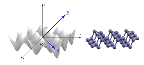
Figure 2: Left: Schematic representation of a corrugation potential in the presence of a tilted perpendicular ($B_{\perp}$) and in-plane ($B_{\parallel}$) magnetic fields. Right: Puckered structure of MBP.

In Eq. (11), we have introduced a corrugation potential along the $xy$-plane having the form $z(x,y)=V\cos(\textrm{K}x)\cos(\textrm{K}^{\prime}y)$ which can be considered as a small perturbation on the surface of MBP (see Fig.2). Here, $\textrm{K}=2\pi/\ell_{x}$ and $\textrm{K}^{\prime}=2\pi/\ell_{y}$, $\ell_{x}$ and $\ell_{y}$ are the length of the corrugation along the $x$ and $y$ directions, respectively. $V$ is the height (amplitude) of the corrugation, $\Theta(B,\theta)=B_{\perp}(\sin\theta+\xi)$, and $\xi=B_{\parallel}/B_{\perp}$. In what follows, the effect of corrugation potential on LLs is treated perturbatively, and assuming $B_{\perp}>B_{\parallel}$ ($\xi<1$), which preserves $C_{2h}$ group invariance of the MBP lattice. More sophisticated analysis can be, in principle, performed following the variational technique Kandemir and Mogulkoc (2010a, b). Considering the modified momentum operators in Eq. (11) and following the same procedure outlined in Sec. II A, the energy eigenvalues of the system can be written as

$$E_{n\lambda} = \overline{E}_{n\lambda}^{0}+\frac{\lambda}{2}\Delta E_{n},$$ (12)

$$\Delta E_{n} = \left(\Delta E_{n}^{x}+\Delta E_{n}^{y}\right)$$

Here, $\overline{E}_{n\lambda}^{0}$ is a modified angle-dependent version of the energy eigenvalues that appeared in Eq. (8), i.e., $\overline{E}_{n\lambda}^{0}=(u_{0}+\lambda\delta)+\lambda\hbar\overline{\omega}_{\lambda}(n+1/2)$, where $\overline{\omega}_{\lambda}=\omega_{\lambda}\cos\theta$ is the modified cyclotron frequency. $\Delta E_{n}^{x}$ and $\Delta E_{n}^{y}$ are the first-order corrections to the energy eigenvalues given by

$$\Delta E_{n}^{i} = \frac{e^{2}B_{\perp}^{2}}{2m^{\lambda}_{i}}\left(\sin\theta+\xi\right)^{2}\frac{V^{2}}{4}\mathbb{G}_{n},$$ (13)

with

$$\mathbb{G}_{n} = \left\langle n_{x}n_{y}\right|\cos^{2}(\textrm{K}x)\cos^{2}(\textrm{K}^{\prime}y)\left|n_{x}n_{y}\right\rangle$$ (14)

being the spatial correlation function defined as

$$\mathbb{G}_{n} = \int_{-\infty}^{\infty}\int_{-\infty}^{\infty}dxdy\Psi_{n_{x}n_{y}}^{*}(x,y)\cos^{2}(\textrm{K}x)\cos^{2}(\textrm{K}^{\prime}y)\Psi_{n_{x}n_{y}}(x,y).$$ (15)

In Eq. (15), $\Psi_{n_{x}n_{y}}(x,y)=\left\langle\mathbf{r}|n_{x}n_{y}\right\rangle$, and

$$\left\langle\mathbf{r}|n_{x}n_{y}\right\rangle = \frac{1}{\sqrt{2^{n_{x}}n_{x}!\sqrt{\pi}}}\frac{1}{\sqrt{2^{n_{y}}n_{y}!\sqrt{\pi}}}\sqrt[4]{\frac{m^{\lambda}_{x}\overline{\omega}_{\lambda}}{\hbar}}\sqrt[4]{\frac{m^{\lambda}_{y}\overline{\omega}_{\lambda}}{\hbar}}$$ (16)

$$\times \exp\left(\frac{-m^{\lambda}_{x}\overline{\omega}_{\lambda}}{2\hbar}x^{2}\right)\exp\left(\frac{-m^{\lambda}_{y}\overline{\omega}_{\lambda}}{2\hbar}y^{2}\right)$$

$$\times H_{n_{x}}\left(\sqrt{\frac{m^{\lambda}_{x}\overline{\omega}_{\lambda}}{\hbar}}x\right)H_{n_{y}}\left(\sqrt{\frac{m^{\lambda}_{y}\overline{\omega}_{\lambda}}{\hbar}}y\right),$$

where $H_{n}$ are the Hermite polynomials (see Appendix A). After taking the integrals in Eq. (15) and considering the assumption $n_{x}=n_{y}=n$, we get (see Appendix for more details)

$$\mathbb{G}_{n} = \left[1+\exp\left(\frac{-\textrm{K}^{2}\hbar}{m^{\lambda}_{x}\overline{\omega}_{\lambda}}\right)L_{n}\left(\frac{2\textrm{K}^{2}\hbar}{m^{\lambda}_{x}\overline{\omega}_{\lambda}}\right)\right]\left[1+\exp\left(\frac{-\textrm{K}^{\prime 2}\hbar}{m^{\lambda}_{y}\overline{\omega}_{\lambda}}\right)L_{n}\left(\frac{2\textrm{K}^{\prime 2}\hbar}{m^{\lambda}_{y}\overline{\omega}_{\lambda}}\right)\right],$$ (17)

where $L_{n}$ are the Laguerre polynomials. To see the oscillatory nature of the Laguerre polynomials, their asymptotic expression can be used, $e^{u/2}L_{n}(u)\approx\left(\pi^{2}nu\right)^{-1/4}\cos\left(2\sqrt{nu}-\pi/4\right)$. For large $n$, $n\rightarrow(E_{F}/\hbar\omega_{\lambda})-1/2$ Vasilopoulos and Peeters (1989); Peeters and Vasilopoulos (1993) and

$$\mathbb{G}_{n} \approx \left[1+\frac{1}{\sqrt{\pi}}\frac{1}{[(\pi\hbar n_{c}/m_{\lambda}\overline{\omega}_{\lambda})-1/2]}\left(\frac{m^{\lambda}_{x}\overline{\omega}_{\lambda}}{2\textrm{K}^{2}\hbar}\right)^{1/4}\cos\left[2\left[\left(\frac{\pi\hbar n_{c}}{m_{\lambda}\overline{\omega}_{\lambda}}-\frac{1}{2}\right)\frac{m^{\lambda}_{x}\overline{\omega}_{\lambda}}{2\textrm{K}^{2}\hbar}\right]^{1/2}-\frac{\pi}{4}\right]\right]$$ (18)

$$\times \left[1+\frac{1}{\sqrt{\pi}}\frac{1}{[(\pi\hbar n_{c}/m_{\lambda}\overline{\omega}_{\lambda})-1/2]}\left(\frac{m^{\lambda}_{y}\overline{\omega}_{\lambda}}{2\textrm{K}^{\prime 2}\hbar}\right)^{1/4}\cos\left[2\left[\left(\frac{\pi\hbar n_{c}}{m_{\lambda}\overline{\omega}_{\lambda}}-\frac{1}{2}\right)\frac{m^{\lambda}_{y}\overline{\omega}_{\lambda}}{2\textrm{K}^{\prime 2}\hbar}\right]^{1/2}-\frac{\pi}{4}\right]\right].$$

Here, $m_{\lambda}=(m_{x}^{\lambda}m_{y}^{\lambda})^{1/2}$ is the cyclotron mass, and $n_{c}=m_{\lambda}E_{F}/\pi\hbar^{2}$ is the carrier concentration.

The density of states (DOS) for quantized energy spectrum can be calculated as

$$D(E) = \frac{1}{S}\sum_{n,\lambda}\delta\left(E-E_{n\lambda}\right)$$ (19)

where $S$ is the area of the MBP unit cell. To calculate DOS, we use the Gaussian functions as an approximation to the Dirac function in Eq. (19), i.e., $\delta\left(E-E_{n\lambda}\right)\approx\left(1/\sigma\sqrt{\pi}\right)\exp\left[-\left(E-E_{n\lambda}\right)^{2}/\sigma^{2}\right]$, with $\sigma$ being the broadening parameter taken to be $\sigma=0.1$ meV.

II.3 Magnetotransport properties

To examine the effect of tilted magnetic field on magnetotransport properties of MBP, we make use of the linear response theory. We consider a strongly quantized regime, in which $\overline{\omega}_{\lambda}\gg\tau^{-1}$, where $\tau$ is the carrier relaxation time. In the presence of the perturbative term in Eq. (12), the carrier velocity along both $x$ and $y$ directions remains zero due to the Landau quantization. In this situation, one can distinguish between the two main contributions to the conductivity tensor, namely, transverse (Hall) $\sigma_{xy}$ and longitudinal (collisional) conductivity $\sigma_{xx}$. The Hall conductivity can be readily evaluated as

$$\sigma_{xy} = g_{s}\frac{e^{2}}{h}\sum_{n=0}^{\infty}\sum_{\lambda=\pm}\left(n+1\right)\left[f\left(E_{n,\lambda}\right)-f\left(E_{n+1,\lambda}\right)\right],$$ (20)

which is a standard expression for conventional 2D electron gas Vasilopoulos (1985); Vasilopoulos and Peeters (1989); Peeters and Vasilopoulos (1992, 1993). Here, $g_{s}=2$ stands for the spin degrees of freedom, and $f\left(E_{n,\lambda}\right)=\left[1+\exp\beta\left(E_{n,\lambda}-E_{F}\right)\right]^{-1}$ is the Fermi-Dirac distribution function, where $E_{F}$ is the Fermi energy, $\beta=1/k_{B}T$ is the inverse temperature in energy units with $k_{B}$ being the Boltzmann constant. It is worth noting that $\sigma_{xy}$ is scattering independent.

The second contribution to the conductivity tensor, i.e., longitudinal conductivity, can be evaluated as Vasilopoulos (1985); Vasilopoulos and Peeters (1989); Peeters and Vasilopoulos (1992, 1993); Vasilopoulos and Van Vliet (1986)

$$\sigma_{xx} = g_{s}\frac{e^{2}}{h}\frac{n^{1/2}_{\mathrm{imp}}\beta}{4\pi^{3/2}\overline{\ell}_{B}}\sum_{n=0}^{\infty}\sum_{\lambda=\pm}U^{\lambda}(2n+1)f\left(E_{n,\lambda}\right)\left[1-f\left(E_{n,\lambda}\right)\right].$$ (21)

Here, we assume scattering on randomly distributed Coulomb impurities with density $n_{\mathrm{imp}}$. Other scattering mechanism, such as scattering on phonons can be neglected in the limit of low temperatures. In Eq. (21), $\overline{\ell}_{B}=\sqrt{\hbar/eB_{\perp}\cos\theta}$ is the magnetic length, and $U^{\lambda}=2\pi e^{2}k_{e}/\epsilon k_{s}^{\lambda}$ is the impurity Coulomb potential for small momentum transfer $q\ll k_{s}$, where $\epsilon$ is the relative dielectric permittivity, $k_{e}=1/4\pi\epsilon_{0}$ is the Coulomb constant, and $k_{s}^{\lambda}=2\pi e^{2}D^{\lambda}_{0}$ is the screening wave vector of electrons (holes) in the Thomas-Fermi approximation Katsnelson (2012) with $D^{\lambda}_{0}=m_{\lambda}/\pi\hbar^{2}$ being DOS in the absence of magnetic field. Eq. (21) represents a collisional contribution to the conductivity $\sigma_{xx}=\sigma_{xx}^{\mathrm{col}}$, which increases with impurity concentration $n_{\mathrm{imp}}$ contrary to the diffusive contribution $\sigma_{xx}^{\mathrm{dif}}\sim 1/n_{\mathrm{imp}}$ Yuan et al. (2015); Liu et al. (2016). This is because impurity scattering in the presence of a magnetic field favors electron hoppings between quantized cyclotron orbits Peeters and Vasilopoulos (1992), thus increasing the conductivity. It is also interesting to note that as long as $\sigma_{xx}^{\mathrm{col}}$ dominates, $\sigma_{xx}$ remains isotropic. We note that in contrast to earlier studies Zhou et al. (2015a), we explicitly take into account impurity- and field-induced broadening of the LLs widthVasilopoulos and Van Vliet (1986). Using Eq. (21), the Hall and longitudinal resistivity can be calculated as $\rho_{xy}=\sigma_{xy}/S$ and $\rho_{xx}=\sigma_{xx}/S$, respectively, where $S=\sigma_{xx}\sigma_{yy}-\sigma_{xy}\sigma_{yx}\approx\sigma_{xy}^{2}$ assuming $\sigma_{xy}\gg\sigma_{xx}$ in sufficiently strong fields. In the following magnetotransport calculations, we use $T=1$ K, $n_{\mathrm{imp}}=10^{12}$ cm^-2, and $\epsilon=1$. The latter corresponds to the case of freestanding non-doped MBP Prishchenko et al. (2017).

III Results and Discussion

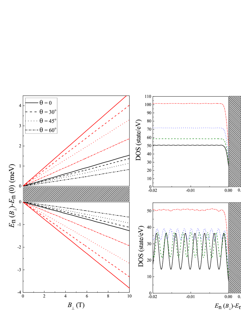
Figure 3: Left panel: Field-dependence of the two first LLs in MBP calculated for different tilt angles $\theta$. Black line corresponds to $n=0$, red line to $n=1$. Right panel: Density of states (DOS) in the vicinity of a gap (shaded area) calculated for $B_{\perp}=5$ T (top) and $B_{\perp}=10$ T (bottom) for different $\theta$ and fixed $\xi=B_{\parallel}/B_{\perp}=0.5$. All cases with $\theta\neq 0$ correspond to the corrugation potential with amplitude $V=1$ Å and lengths $l_{1}=l_{2}=250$ Å.

We first examine evolution of LLs in MBP considering tilted magnetic field in the presence of a corrugation potential. Since we use a perturbative approach to describe the effect of angle-dependent magnetic field [Eq. (12)], the product $(B_{\perp}V)^{2}$ must not be too large to ensure validity of the approach, that is to satisfy $\Delta E_{n\lambda}\ll E_{n}$. This condition holds for $B_{\perp}<10$ T and $V<5$ Å considered in this work. Unless stated otherwise, we consider fixed ratio $\xi=B_{\parallel}/B_{\perp}=0.5$, and the corrugation length along both directions $\ell_{1}=\ell_{2}=250$ Å, which is an order of intrinsic ripples length in graphene Meyer et al. (2007); Fasolino et al. (2007). The case $\theta=0$ is evaluated for $V=0$ to be consistent with the results of earlier works Pereira and Katsnelson (2015); Zhou et al. (2015a).

In the left panel of Fig. 3, we show the Landau level diagram calculated for both electron and hole states for different values of tilt angle $\theta$, and fixed amplitude of the corrugation potential $V=1$ Å. One can see that energies of LLs decrease with $\theta$, while the linearity of the curves is preserved in the regime of relatively small corrugations and not too strong magnetic fields. The effect of the tilt angle on LLs is twofold. While $B_{\perp}$ confines the motion of charge carriers in the $xy$ plane, changing the magnetic field direction increases the cyclotron radius in the $xy$ plane due to the $\mathrm{cos}\theta$ factor in $\overline{\omega}_{\lambda}$. As a result, the LL energies $E_{n}$ decrease with $\theta$, which effectively correspond to a smaller magnetic field. This effect is partially compensated by the presence of the corrugation potential, which provides an additional contribution $\Delta E_{n}$ to $E_{n}$ [Eq. (13)]. As can be inferred from Fig. 3, the main contribution to LLs comes from the first term, $\overline{E}_{n\lambda}^{0}$ in Eq. (12), which is strongly dependent on the perpendicular component of the out-of-plane magnetic field $B_{\perp}\cos\theta$. The effect of the second term, $\Delta E_{n}$ in Eq. (12) is small for corrugations as low as $V=1$ Å. The effect of tilted magnetic field on the electronic spectrum can be seen also from DOS shown for different tilt angles at $B_{\perp}=5$ T and $B_{\perp}=10$ T (right panel of Fig. 3). At $\theta\neq 0$, the energy spacing between LLs becomes smaller, which leads to more dense electronic states and larger DOS. A similar effect of tilted magnetic field on LLs of graphene was reported previouslyKandemir (2010); Krstajić (2013). For larger values of $B_{\perp}$, the energy spacing between LLs decreases, which gives rise to more pronounced oscillations in DOS shown in Fig. 3 for $B_{\perp}=10$ T.

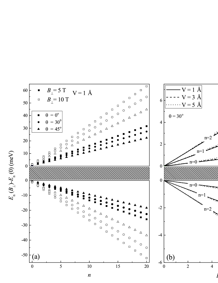
Figure 4: Energies of LLs shown as a function of the level index $n$ for different tilt angles $\theta$, magnetic fields $B_{\perp}$ and corrugation heights $V$. Shaded area is an energy gap.

In Fig. 4(a), the index ($n$) dependence of LLs is shown in the presence of tilted magnetic field for $V=1$ Å. LLs splitting of electron and hole states is different because of the electron-hole asymmetry and unequal effective masses. In Fig. 4(b), the magnetic field ($B_{\perp}$) dependence of LLs is shown for different corrugation heights at $\theta=30$ Å. One can see pronounced deviations from the linear behavior, which become especially clear for $V=5$ Å and $B_{\perp}=10$ T. In the chosen range of parameters, these deviations do not exceed $\hbar\overline{\omega}_{\lambda}(n+1/2)$, demonstrating the validity of the perturbative approach. The observed nonlinearity is a manifestation of long-range structural corrugations. Although at relatively weak fields, first-order correction to the LLs energy is quadratic in $V$ [Eq. (13)], the dependence at large fields may be different. Particularly, we do not exclude oscillatory behavior in this regime.

Fermi energy as a function of magnetic field is shown in Fig. 5 for different electron concentrations $n_{c}$. For fixed Fermi energy, carrier concentration can be calculated by the formula, $n_{c}=\int_{0}^{E_{F}}D\left(E\right)dE$. Here, we see the magnetic field dependence of fixed Fermi energies for different carrier concentrations.

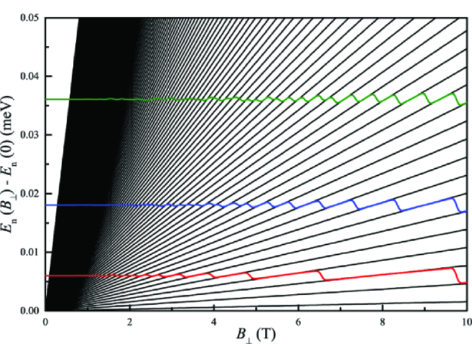
Figure 5: Fermi energy as a function of magnetic field, $B_{\perp}$, for $n_{c}=1\times 10^{16}$ m^-2 (red), $n_{c}=3\times 10^{16}$ m^-2 (blue), and $n_{c}=6\times 10^{16}$ m^-2 (green).

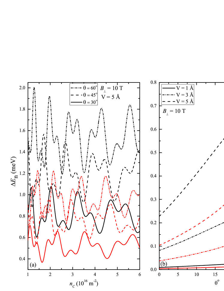
Figure 6: Tilted magnetic field contribution to the LL oscillations ($\Delta E_{n}$) calculated with respect to (a) carrier concentration $n_{c}$ for different $\theta$, and (b) $\theta$ for different $V$ at $n_{c}=1\times 10^{16}$ m^-2. In all cases $\ell_{1}=\ell_{2}=100$ Å and $\xi=0.5$. Black and red lines correspond to the electron and hole states, respectively.

To gain insight into the role of other model parameters on the LL spectrum, we analyze $\Delta E_{n}$ in more detail. In Fig. 6(a), $\Delta E_{n}$ is shown both for electrons and holes as a function of the carrier concentration $n_{c}$ calculated for different tilt angles $\theta$ at $B_{\perp}=10$ T. It can be seen that $\Delta E_{n}$ exhibits oscillations with $n_{c}$, and its amplitude increases for larger $\theta$. This behavior is attributed to the $\sin\theta$ factor in $\Delta E_{n}$ [Eq. (13)]. The hole states turn out to be less affected by the magnetic field direction, which is due to the higher cyclotron mass. In Fig. 6(b), we show $\Delta E_{n}$ as a function of $\theta$ calculated for different $V$. According to Eq. (13), $\Delta E_{n}\sim V^{2}(\sin\theta+\xi)^{2}$, meaning that the nonlinear effects in the spectrum of LLs increase both with $V$ and $\theta$. At small $\theta$, $\Delta E$ raises linearly, whereas at larger $\theta$, $\Delta E_{n}$ demonstrates a quadratic behavior.

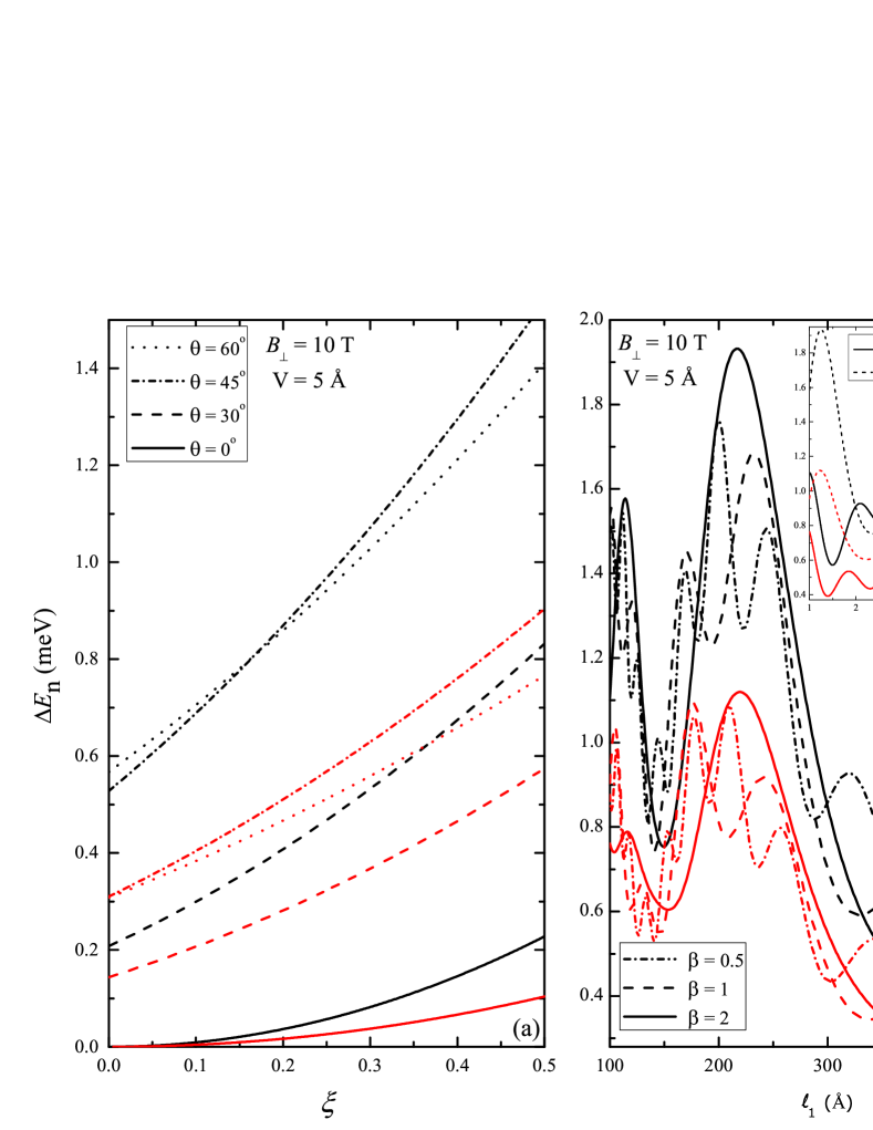
Figure 7: LL oscillations ($\Delta E_{n}$) calculated with respect to (a) $\xi=B_{\parallel}/B_{\perp}$ for different $\theta$, and (b) $\ell_{1}$ for different $\beta=\ell_{2}/\ell_{1}$ at $n_{c}=1\times 10^{16}$ m^-2. The inset shows the dependence of $\Delta E_{n}$ on the carrier concentration $n_{c}$ for $\ell_{1}=2\ell_{2}=500$Å and $\ell_{2}=2\ell_{1}=500$Å. Black and red lines correspond to the electron and hole states, respectively.

In Fig. 7(a), we show the effect of a parallel magnetic field $B_{\parallel}$ by calculating the dependence of $\Delta E_{n}$ on the dimensionless parameter $\xi=B_{\parallel}/B_{\perp}$. One can see the expected from Eq. (13) $\Delta E_{n}\sim\xi^{2}$ behavior, suggesting that at large $\xi$ the in-plane field might play a role in the energy spectrum of corrugated MBP samples. The absolute effect of $B_{\parallel}$ is, however, not large and can hardly be detected experimentally under realistic field strengths and corrugation amplitudes. A similar effect of $B_{\parallel}$ on LLs was also reported previously in the context of bilayer graphene Hyun et al. (2012). Fig. 7(b) shows the effect of the corrugation length $\ell_{1}$ as well as its anisotropy $\beta=\ell_{2}/\ell_{1}$ on $\Delta E_{n}$. In this case, $\Delta E_{n}$ exhibits a complicated oscillatory behavior. Keeping in mind anisotropic ripple formation typical to MBPKou et al. (2015), we also examine $\Delta E_{n}$ as a function of $n_{c}$ for anisotropic corrugation patterns [see inset of Fig. 7(b)]. Depending on the corrugation direction, the behavior of LLs is significantly different. One can see, however, that $\Delta E_{n}$ remains weakly affected by a particular corrugation pattern as well as by the corrugation length.

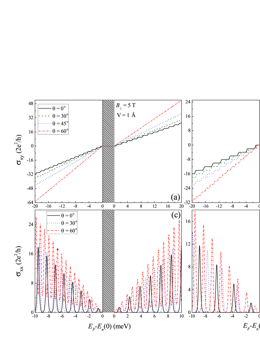
Figure 8: Hall conductivity ($\sigma_{xy}$) calculated for (a) $B_{\perp}=5$ T, (b) $B_{\perp}=10$ T, and longitudinal conductivity ($\sigma_{xx}$) calculated for (c) $B_{\perp}=5$ T, (d) $B_{\perp}=10$ T. Shaded area correspond to a gap in the energy spectrum.

We now turn to the results of our magnetotransport calculations to see whether weak effects induced by the corrugation could be observed experimentally. The Hall ($\sigma_{xy}$) and longitudinal ($\sigma_{xx}$) conductivities are shown for different tilt angles in Fig. 8. For Fermi energies in the gap region between the valence and conduction states, dc conductivity is obviously zero due to the absence of charge carriers. Beyond the gap region, $\sigma_{xy}$ exhibits distinct plateaus, arising from the discrete nature of the LL spectrum [Fig. 8(a)]. The Hall conductivity increases by $2e^{2}/h$ for each level forming the integer Hall plateaus indexed as $0,\pm 2,\pm 4,\pm 6...$. It can be seen that $\sigma_{xy}$ increases with tilt angle, which is attributed to larger DOS caused by more dense LLs (cf. Fig. 3). For the same reason, $\sigma_{xy}$ becomes smaller in stronger fields [Fig. 8(b)]. At sufficiently small $V$, $\sigma_{xy}\sim(B_{\perp}\cos\theta)^{-1}$. The longitudinal conductivity $\sigma_{xx}$ exhibits oscillatory behavior typical to the Shubnikov-de Haas (SdH) oscillations, as shown in Figs. 8(c) and (d). $\sigma_{xx}$ also increases with $\theta$ yet more slowly than $\sigma_{xy}$, because in this case $\sigma_{xx}\sim(B_{\perp}\cos\theta)^{-1/2}$ due to a factor $\overline{\ell}_{B}$ in the denominator of Eq. (21). We note that the effect of in-plane magnetic field ($B_{\parallel}$) and the corrugation lengths ($\ell_{1}$ and $\ell_{2}$) are negligible in the context of magnetotransport properties of MBP and, therefore, not presented here. The role of the corrugation amplitude is analyzed below.

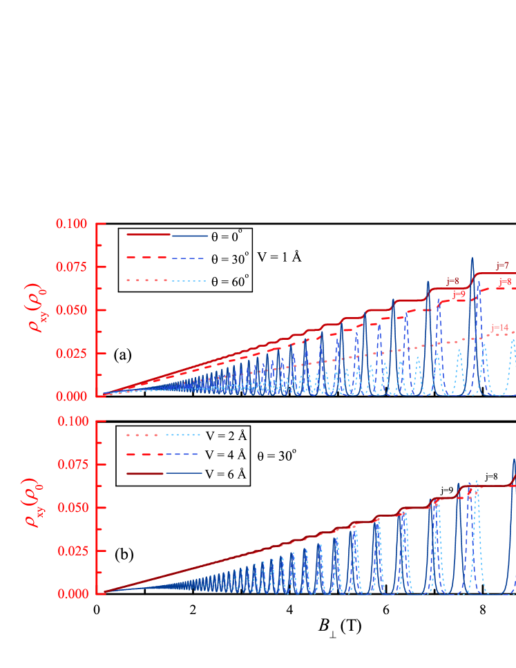
Figure 9: Hall resistivity ($\rho_{xy}$) and longitudinal resistivity ($\rho_{xx}$) versus magnetic field, $B_{\perp}$ for different tilt angles $\theta$. The case of electron doping with $n_{c}\approx 3\times 10^{16}$ m^-2 is considered. $\rho_{0}=h/2e^{2}$ is the resistivity unit.

In Fig. 9(a), the Hall $\rho_{xy}$ and longitudinal $\rho_{xx}$ resistivity are shown as a function of magnetic field calculated at different $\theta$ for the case of electron doping $n_{c}\approx 3\times 10^{16}$ m^-2 and $V=1$ Å. The behavior of $\rho_{xy}$ is closely related to $\sigma_{xy}$ shown in Fig. 8. As expected, $\rho_{xy}$ increases linearly with $B_{\perp}$, while larger $\theta$ correspond to effectively weaker fields. At large fields, $\rho_{xy}$ becomes quantized increasing by the unit of $\rho_{0}=h/2e^{2}$. For a given magnetic field, the Hall plateaus observed at different $\theta$ correspond to different filling factors $j$. The filling factors increase with $\theta$, meaning that the effect of the tilt angle is opposite to that of the Fermi energy, i.e., larger $\theta$ corresponds to shifting the position of the Hall plateaus toward smaller $E_{F}$ and vice versa. Similar effect of tilted magnetic field on resistivities was reported for grapheneKrstajić (2013). As can be seen from Fig. 9(a), the behavior of $\rho_{xx}$ is also similar to $\sigma_{xx}$, exhibiting pronounced SdH oscillations as well as a $\theta$-dependence of the peak amplitudes. One of the most interesting result is presented in Fig. 9(b), which shows the effect of the corrugation amplitudes $V$ on $\rho_{xy}$ and $\rho_{xx}$ calculated for a fixed $\theta$. Although the effect of $V$ is less pronounced compared to $\theta$, it becomes clearly seen at fields $B_{\perp}>5$ T. Larger $V$ shift the Hall plateaus in $\rho_{xy}$ as well as SdH oscillation peaks in $\rho_{xx}$ toward weaker magnetic fields. For sufficiently strong fields, the difference in corrugation amplitudes of a few Å results in a notable contraction of the $\rho(B_{\perp})$ spectrum along the field axis reaching 0.5 T at $B_{\perp}\sim 8$ T. Given that a realistic corrugation pattern would be represented by a superposition of different corrugation amplitudes, we expect a broadening of the SdH peaks increasing with $B_{\perp}$ under experimental conditions. Although such a behavior is typical to experimentally measured longitudinal and Hall resistivity in few-layer BPTayari et al. (2015); Li et al. (2015, 2016); Long et al. (2016, 2017), it is usually attributed to the Zeeman spin-splitting, well described by the standard Lifshitz-Kosevich formula for 2D resistivity. To reveal the effect of corrugations in the resistivity measurements, the broadening must increase with tilt angle, which is apparently not observed in known experiments on few-layer BP. The resolution of the available experimental spectra also does not allow us to observe nonlinear effects in the SdH oscillations. We note, however, that the existing magnetotransport measurements has been performed on a few-layer BP, which should be significantly less affected by the structural corrugations compared to single-layer samples.

IV Conclusions

In summary, we studied the effects of tilted magnetic field and long-range structural corrugations on LLs and magnetotransport properties of MBP. We considered an analytical model and obtained first-order corrections to the LL energies induced by corrugations in the long-wavelength limit. The energies of LLs are found to be expectedly decreasing with the tilt angle due to the $\cos\theta$ factor in the modified cyclotron frequency. At sufficiently strong fields, however, the corrugation potential induces nonlinear deviations in the dependence of LL energies on magnetic field. We find that these deviations are predominantly affected by the corrugation amplitude, whereas the corrugation length and its specific direction are less relevant. We also examined the magnetotransport properties of MBP in the presence of corrugations under tilted magnetic field within the scheme of linear response theory. Overall, the tilt angle modifies the resistivity spectra considerably, effectively reducing the magnetic field strength. In the presence of long-range corrugations, we find that both Hall and longitudinal resistivity spectra display: (i) a shift toward weaker magnetic fields, and (ii) additional broadening of the SdH peaks increasing with magnetic field, not related to the Zeeman splitting. The obtained effects are noticeable even at moderate ($B<10$ T) fields, which allows us to expect that they might be observable experimentally for MBP samples deposited on sufficiently corrugated (e.g., SiO₂) substrates.

References

Appendix A Derivation of energy eigenvalues in the presence of magnetic field

In the symmetric gauge, energy eigenvalues of the Hamiltonian given by Eq. (1) can be expressed as

$$E_{n\lambda}^{0} = u_{0}+\lambda\delta+(\bar{\eta}_{x}+\lambda\bar{\gamma}_{x})\left[\frac{m^{\lambda}_{x}\hbar\omega_{\lambda}}{2}\langle(b_{x}^{\dagger}+b_{x})^{2}\rangle-\left(\frac{eB}{2}\right)^{2}\frac{\hbar}{2m^{\lambda}_{y}\omega_{\lambda}}\langle(b_{y}^{\dagger}-b_{y})^{2}\rangle\right]$$ (22)

$$+ (\bar{\eta}_{y}+\lambda\bar{\gamma}_{y}+\lambda\frac{\bar{\chi}^{2}}{2\delta})\left[\frac{m^{\lambda}_{y}\hbar\omega_{\lambda}}{2}\langle(b_{y}^{\dagger}+b_{y})^{2}\rangle-\left(\frac{eB}{2}\right)^{2}\frac{\hbar}{2m^{\lambda}_{x}\omega_{\lambda}}\langle(b_{x}^{\dagger}-b_{x})^{2}\rangle\right]$$

$$- (\bar{\eta}_{x}+\lambda\bar{\gamma}_{x})\left[ieB\sqrt{\frac{m^{\lambda}_{x}\hbar\omega_{\lambda}}{2}}\sqrt{\frac{\hbar}{2m^{\lambda}_{y}\omega_{\lambda}}}\langle(b_{x}^{\dagger}+b_{x})(b_{y}^{\dagger}-b_{y})\rangle\right]$$

$$+ (\bar{\eta}_{y}+\lambda\bar{\gamma}_{y}+\lambda\frac{\bar{\chi}^{2}}{2\delta})\left[ieB\sqrt{\frac{m^{\lambda}_{y}\hbar\omega_{\lambda}}{2}}\sqrt{\frac{\hbar}{2m^{\lambda}_{x}\omega_{\lambda}}}\langle(b_{y}^{\dagger}+b_{y})(b_{x}^{\dagger}-b_{x})\rangle\right],$$

where $\langle...\rangle$ corresponds to expectation values between the oscillator states, $|n_{x}n_{y}\rangle$. Creation and annihilation operators satisfy the commutation relation, $\left[b_{i},b_{j}^{\dagger}\right]=\delta_{ij}$ and they have eigenvalues $b_{x(y)}|n_{x}n_{y}\rangle=\sqrt{n_{x(y)}}|n_{x-1(x)}n_{y(y-1)}\rangle$ and $b_{x(y)}^{\dagger}|n_{x}n_{y}\rangle=\sqrt{n_{x(y)}+1}|n_{x+1(x)}n_{y(y+1)}\rangle$. Furthermore, number operators ($\hat{n}_{x}=b_{x}^{\dagger}b_{x}$ and $\hat{n}_{y}=b_{y}^{\dagger}b_{y}$) have the following eigenvalues

$$\hat{n}_{x}|n_{x}n_{y}\rangle = n_{x}|n_{x}n_{y}\rangle$$

$$\hat{n}_{y}|n_{x}n_{y}\rangle = n_{y}|n_{x}n_{y}\rangle.$$ (23)

Here, $n_{x}$ and $n_{y}$ are positive integers, i.e., $n_{x(y)}=0,1,2...$. The last two terms in Eq. (22) correspond to the angular momentum operator $L_{z}$, which satisfies the eigenvalue equation $L_{z}|n_{x}n_{y}\rangle=\hbar\left(n_{y}-n_{x}\right)|n_{x}n_{y}\rangle$. Here, $n_{y}-n_{x}=m$ where $m$ is the magnetic quantum number. Using the assumption $n_{x}=n_{y}=n$, this term vanishes and Eq.(22) leads to Eq. (7). Further details can be found in Refs. de Brito and Nazareno, 2007 and Messiah, 1961. By the inclusion of tilted magnetic field and corrugation potential with the modified symmetric gauge, square of the momentum operators is given by Eq. (11). Similar method can be followed for the evaluation of the energy eigenvalues. Assuming $n_{x}=n_{y}=n$, non-zero elements of the energy eigenvalues can be written as,

$$E_{n\lambda}^{0} = u_{0}+\lambda\delta+(\bar{\eta}_{x}+\lambda\bar{\gamma}_{x})\left[\frac{m^{\lambda}_{x}\hbar\overline{\omega}_{\lambda}}{2}\langle(b_{x}^{\dagger}+b_{x})^{2}\rangle-\left(\frac{eB_{\perp}\cos\theta}{2}\right)^{2}\frac{\hbar}{2m^{\lambda}_{y}\overline{\omega}_{\lambda}}\langle(b_{y}^{\dagger}-b_{y})^{2}\rangle\right]$$ (24)

$$+ (\bar{\eta}_{y}+\lambda\bar{\gamma}_{y}+\lambda\frac{\bar{\chi}^{2}}{2\delta})\left[\frac{m^{\lambda}_{y}\hbar\overline{\omega}_{\lambda}}{2}\langle(b_{y}^{\dagger}+b_{y})^{2}\rangle-\left(\frac{eB_{\perp}\cos\theta}{2}\right)^{2}\frac{\hbar}{2m^{\lambda}_{x}\overline{\omega}_{\lambda}}\langle(b_{x}^{\dagger}-b_{x})^{2}\rangle\right]$$

$$+ (\bar{\eta}_{x}+\lambda\bar{\gamma}_{x})\left[\frac{e^{2}B_{\perp}^{2}\left(\sin\theta+\xi\right)^{2}}{2}\frac{V^{2}}{4}\mathbb{G}_{n}\right]+(\bar{\eta}_{y}+\lambda\bar{\gamma}_{y}+\lambda\frac{\bar{\chi}^{2}}{2\delta})\left[\frac{e^{2}B_{\perp}^{2}\left(\sin\theta+\xi\right)^{2}}{2}\frac{V^{2}}{4}\mathbb{G}_{n}\right],$$

Here, first two terms result in $\bar{E}_{n\lambda}^{0}$ appearing in Eq. (12), which is a modified counterpart of Eq. (8) with $\cos\theta$ factor. The last term corresponds to the first-order correction to the energy eigenvalues given by Eq. (13). In turn, spatial correlation function $\mathbb{G}_{n}$ can be written using Eqs. (15) and (16) as

$$\mathbb{G}_{n} = \left[\frac{1}{2^{n}n!\sqrt{\pi}}\sqrt{\frac{m^{\lambda}_{x}\overline{\omega}_{\lambda}}{\hbar}}\int_{-\infty}^{\infty}dx\cos^{2}(\textrm{K}x)\left|H_{n}\left(\sqrt{\frac{m^{\lambda}_{x}\overline{\omega}_{\lambda}}{\hbar}}x\right)\right|^{2}\right]$$ (25)

$$\times \left[\frac{1}{2^{n}n!\sqrt{\pi}}\sqrt{\frac{m^{\lambda}_{y}\overline{\omega}_{\lambda}}{\hbar}}\int_{-\infty}^{\infty}dy\cos^{2}(\textrm{K}^{\prime}y)\left|H_{n}\left(\sqrt{\frac{m^{\lambda}_{y}\overline{\omega}_{\lambda}}{\hbar}}y\right)\right|^{2}\right].$$

Integrals in Eq. (25) can be taken by using the identity Gradshteyn and Ryzhik (2014),

$$\int_{0}^{\infty}d\alpha\exp\left(-\alpha^{2}\right)\left[H_{n}\left(\alpha\right)\right]^{2}\cos\left(\sqrt{2}\beta\alpha\right) = 2^{n-1}\sqrt{\pi}n!\exp\left(-\beta^{2}/2\right)L_{n}\left(\beta^{2}\right).$$ (26)

Here, $H_{n}(x)$ and $L_{n}(x)$ are the Hermite and the Laguerre polynomials, respectively. By using trigonometric identities [$\cos^{2}\theta=(1+\cos 2\theta)/2$] and Eq. (26), one can recast spatial correlation function in Eq. (25) as Eq. (17).

Appendix B Tight-binding description of magnetic field

For the tight-binding calculations, we consider the model proposed in Ref. Rudenko and Katsnelson, 2014. The model consists of five hopping parameters between the $p_{z}$-like orbitals of phosphorus atoms. In the presence of external magnetic field the hopping parameters acquire a Peierls phase Graf and Vogl (1995). The corresponding hopping between the atoms at $\mathbf{r}_{1}$ and $\mathbf{r}_{2}$ become

$$t_{\mathbf{r}_{1},\mathbf{r}_{2}}\rightarrow t_{\mathbf{r}_{1},\mathbf{r}_{2}}\mathrm{exp}\left({ie/\hbar\int_{\mathbf{r}_{1}}^{\mathbf{r}_{2}}\mathbf{A}\cdot d\mathbf{l}}\right),$$ (27)

where $\mathbf{A}$ is the vector potential. For a homogeneous perpendicular magnetic field applied in the $z$ direction $B_{\perp}$, we choose the Landau gauge A=(0,$B_{\perp}x$,0). To preserve translation invariance of the system, the magnetic flux $\Phi$ through each unit cell should be chosen as a rational multiply of the flux quantum $\Phi_{0}=e/h$ Graf and Vogl (1995). In the case of MBP, the magnetic flux through each cell is

$$\Phi=(e/h)\frac{B_{\perp}{a}_{1}{a}_{2}}{2},$$ (28)

where $a_{1}$ and $a_{2}$ are lattice vectors in the $x$ and $y$ directions. In practice, it is convenient to consider a supercell composed of $q$ unit cells in the $x$-direction, such that $\Phi=\Phi_{0}/q$ Jiang et al. (2016). Therefore, low values of $B$ require large supercell meaning that the dimensionality of the tight-binding Hamiltonian increases as $B$ decreases. The LL are obtained by diagonalizing the Hamiltonian at the center ($\Gamma$ point) of the Brillouin zone.

For a perfectly planar atom-thick 2D material like graphene the in-plane magnetic flux through its structure is zero. This is generally not the case for 2D materials with finite thickness like bilayer graphene Hyun et al. (2012). Here, for the puckered structure of MBP, the in-plane magnetic field induces a phase difference between the top and bottom sublayers of phosphorus atoms, which depends on the MBP thickness $d=2.1$ Å. To study the effect of in-plane magnetic field on the electronic properties of MBP, we consider the in-plane field ($B_{\parallel}$) together with perpendicular magnetic field $(B_{\perp})$ using the vector potential A=(0,$B_{\perp}x$-$B_{\parallel}z$,0) and A=($B_{\parallel}z$,$B_{\perp}x$,0) for $x$- and $y$-directions of $B_{\parallel}$, respectively. Since there is no periodicity in the $z$-direction, the in-plane field does not produce any quantization due to the confinement of charge carriers within the $xy$ plane. However, it gives rise to field-dependent shifts of energy levels. In Fig. 10, the contribution of in-plane field [$\Delta E^{\mathrm{TB}}=E(B_{\perp},B_{\parallel})-E(B_{\perp},0$)] to the LL energies is shown for moderate values of $B_{\parallel}$ applied along both $x$- and $y$-directions. Due to the relatively low buckling ($d=2.1$ Å) and insignificant modification of tight-binding parameters (only $t_{1}$ and $t_{3}$ hoppings are primarily affected), the in-plane magnetic field has a negligible effect on LLs (order of $10^{-5}$ meV). This result is similar to bilayer graphene Hyun et al. (2012), where noticeable changes appear only for $B_{\parallel}>50$ T. Here, however, one can see the anisotropy of contribution due to the direction-dependent effective masses in MBP. We also analyzed the $n$ dependence of $\Delta E^{\mathrm{TB}}$ (not shown here) and conclude that the effect of $B_{\parallel}$ is almost uniform and the $n$ dependence can be considered as negligible.

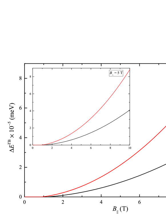
Figure 10: The contribution of in-plane field ($B_{\parallel}$) to the LL energies $\Delta E^{\mathrm{TB}}$ calculated for $B_{\perp}=1$ T and $B_{\perp}=5$ T (inset) for $n=0$.

References

- Novoselov et al. (2004) K. S. Novoselov, A. K. Geim, S. V. Morozov, D. Jiang, Y. Zhang, S. V. Dubonos, I. V. Grigorieva, and A. A. Firsov, “Electric field effect in atomically thin carbon films,” Science 306, 666 (2004).
- Vogt et al. (2012) P. Vogt, P. De Padova, C. Quaresima, J. Avila, E. Frantzeskakis, M. Carmen Asensio, A. Resta, B. Ealet, and G. Le Lay, “Silicene: Compelling experimental evidence for graphenelike two-dimensional silicon,” Phys. Rev. Lett. 108, 155501 (2012).
- Dávila et al. (2014) M. E. Dávila, L. Xian, S. Cahangirov, A. Rubio, and G. Le Lay, “Germanene: a novel two-dimensional germanium allotrope akin to graphene and silicene,” New J. Phys. 16, 095002 (2014).
- Bampoulis et al. (2014) P. Bampoulis, L. Zhang, A. Safaei, R. van Gastel, B. Poelsema, and H. J . W. Zandvliet, “Germanene termination of Ge2Pt crystals on Ge(110),” J. Phys. Condens. Matter 26, 442001 (2014).
- Zhang et al. (2016) L. Zhang, P. Bampoulis, A. N. Rudenko, Q. Yao, A. van Houselt, B. Poelsema, M. I. Katsnelson, and H. J. W. Zandvliet, “Structural and Electronic Properties of Germanene on MoS2,” Phys. Rev. Lett. 116, 256804 (2016).
- Zhu et al. (2015) F.-F. Zhu, W.-J. Chen, Y. Xu, C.-L. Gao, D.-D. Guan, C.-H. Liu, D. Qian, S.-C. Zhang, and J.-F. Jia, “Epitaxial growth of two-dimensional stanene,” Nat. Mater. 14, 1020 (2015).
- Wang et al. (2012) Q. H. Wang, K. Kalantar-Zadeh, A. Kis, J. N. Coleman, and M. S. Strano, “Electronics and optoelectronics of two-dimensional transition metal dichalcogenides,” Nat. Nanotech. 7, 699 (2012).
- Jariwala et al. (2014) D. Jariwala, V. K. Sangwan, L. J. Lauhon, T. J. Marks, and M. C. Hersam, “Emerging Device Applications for Semiconducting Two-Dimensional Transition Metal Dichalcogenides,” ACS Nano 8, 1102 (2014).
- Ling et al. (2015) X. Ling, H. Wang, S. Huang, F. Xia, and M. S. Dresselhaus, “The renaissance of black phosphorus,” Proc. Natl. Acad. Sci. U.S.A. 112, 4523 (2015).
- Castellanos-Gomez (2015) A. Castellanos-Gomez, “Black Phosphorus: Narrow Gap, Wide Applications,” J. Phys. Chem. Lett. 6, 4280 (2015).
- Carvalho et al. (2016) A. Carvalho, M. Wang, X. Zhu, A. S. Rodin, H. Su, and A. H. Castro Neto, “Phosphorene: from theory to applications,” Nat. Rev. Mater. 1, 16061 (2016).
- Koenig et al. (2014) S. P. Koenig, R. A. Doganov, H. Schmidt, A. H. Castro Neto, and B. Özyilmaz, “Electric field effect in ultrathin black phosphorus,” Appl. Phys. Lett. 104, 103106 (2014).
- Liu et al. (2014) H. Liu, A. T. Neal, Z. Zhu, Z. Luo, X. Xu, D. Tománek, and P. D. Ye, “Phosphorene: An Unexplored 2D Semiconductor with a High Hole Mobility,” ACS Nano 8, 4033 (2014).
- Li et al. (2014) L. Li, Y. Yu, G. J. Ye, Q. Ge, X. Ou, H. Wu, D. Feng, X. H. Chen, and Y. Zhang, “Black phosphorus field-effect transistors,” Nat. Nanotech. 9, 372 (2014).
- Tran et al. (2014) V. Tran, R. Soklaski, Y. Liang, and L. Yang, “Layer-controlled band gap and anisotropic excitons in few-layer black phosphorus,” Phys. Rev. B 89, 235319 (2014).
- Rudenko et al. (2015) A. N. Rudenko, S. Yuan, and M. I. Katsnelson, “Toward a realistic description of multilayer black phosphorus: From approximation to large-scale tight-binding simulations,” Phys. Rev. B 92, 085419 (2015).
- Qiao et al. (2014) J. Qiao, X. Kong, Z.-X. Hu, F. Yang, and W. Ji, “High-mobility transport anisotropy and linear dichroism in few-layer black phosphorus,” Nat. Commun. 5, 4475 (2014).
- Xia et al. (2014) F. Xia, H. Wang, and Y. Jia, “Rediscovering black phosphorus as an anisotropic layered material for optoelectronics and electronics,” Nat. Commun. 5, 4458 (2014).
- Wang et al. (2015) X. Wang, A. M. Jones, K. L. Seyler, V. Tran, Y. Jia, H. Zhao, H. Wang, L. Yang, X. Xu, and F. Xia, “Highly anisotropic and robust excitons in monolayer black phosphorus,” Nat. Nanotech. 10, 517 (2015).
- Low et al. (2014) T. Low, R. Roldán, H. Wang, F. Xia, P. Avouris, L. M. Moreno, and F. Guinea, “Plasmons and Screening in Monolayer and Multilayer Black Phosphorus,” Phys. Rev. Lett. 113, 106802 (2014).
- Nemilentsau et al. (2016) A. Nemilentsau, T. Low, and G. Hanson, “Anisotropic 2D Materials for Tunable Hyperbolic Plasmonics,” Phys. Rev. Lett. 116, 066804 (2016).
- Mermin (1968) N. D. Mermin, “Crystalline order in two dimensions,” Phys. Rev. 176, 250 (1968).
- Meyer et al. (2007) J. C. Meyer, A. K. Geim, M. I. Katsnelson, K. S. Novoselov, T. J. Booth, and S. Roth, “The structure of suspended graphene sheets,” Nature 446, 60 (2007).
- Fasolino et al. (2007) A. Fasolino, J. H. Los, and M. I. Katsnelson, “Intrinsic ripples in graphene,” Nat. Mater. 6, 858 (2007).
- de Juan et al. (2007) F. de Juan, A. Cortijo, and M. A. H. Vozmediano, “Charge inhomogeneities due to smooth ripples in graphene sheets,” Phys. Rev. B 76, 165409 (2007).
- Isacsson et al. (2008) A. Isacsson, L. M. Jonsson, J. M. Kinaret, and M. Jonson, “Electronic superlattices in corrugated graphene,” Phys. Rev. B 77, 035423 (2008).
- Guinea et al. (2008a) F. Guinea, M. I. Katsnelson, and M. A. H. Vozmediano, “Midgap states and charge inhomogeneities in corrugated graphene,” Phys. Rev. B 77, 075422 (2008a).
- Guinea et al. (2008b) F. Guinea, B. Horovitz, and P. Le Doussal, “Gauge field induced by ripples in graphene,” Phys. Rev. B 77, 205421 (2008b).
- Cortijo and Vozmediano (2009) A. Cortijo and M. A. H. Vozmediano, “Minimal conductivity of rippled graphene with topological disorder,” Phys. Rev. B 79, 184205 (2009).
- Costamagna et al. (2010) S. Costamagna, O. Hernandez, and A. Dobry, “Spectral gap induced by structural corrugation in armchair graphene nanoribbons,” Phys. Rev. B 81, 115421 (2010).
- Meyer et al. (2009) J. C. Meyer, A. Chuvilin, G. Algara-Siller, J. Biskupek, and U. Kaiser, “Selective sputtering and atomic resolution imaging of atomically thin boron nitride membranes,” Nano Lett. 9, 2683 (2009).
- Brivio et al. (2011) J. Brivio, D. T. L. Alexander, and A. Kis, “Ripples and Layers in Ultrathin MoS2 Membranes,” Nano Lett. 11, 5148 (2011).
- Miro et al. (2013) P. Miro, M. Ghorbani-Asl, and T. Heine, “Spontaneous Ripple Formation in MoS2 Monolayers: Electronic Structure and Transport Effects,” Adv. Mater. 25, 5473 (2013).
- Kou et al. (2015) L. Kou, Y. Ma, S. C. Smith, and C. Chen, “Anisotropic ripple deformation in phosphorene,” J. Phys. Chem. Lett. 6, 1509 (2015).
- Zhou et al. (2016) Y. Zhou, L. Yang, X. Zu, and F. Gao, “Spontaneous ripple formation in phosphorene: electronic properties and possible applications,” Nanoscale 8, 11827 (2016).
- Wang et al. (2016) G. Wang, G. C. Loh, R. Pandey, and S. P. Karna, “Out-of-plane structural flexibility of phosphorene,” Nanotechnology 27, 055701 (2016).
- Ishigami et al. (2007) M. Ishigami, J. H. Chen, W. G. Cullen, M. S. Fuhrer, and E. D. Williams, “Atomic Structure of Graphene on SiO2,” Nano Lett. 7, 1643 (2007).
- Geringer et al. (2009) V. Geringer, M. Liebmann, T. Echtermeyer, S. Runte, M. Schmidt, R. Rückamp, M. C. Lemme, and M. Morgenstern, “Intrinsic and extrinsic corrugation of monolayer graphene deposited on ,” Phys. Rev. Lett. 102, 076102 (2009).
- Lui et al. (2009) C. H. Lui, Li Liu, K. F. Mak, G. W. Flynn, and T. F. Heinz, “Ultraflat graphene,” Nature 462, 339 (2009).
- Chen et al. (2015) X. Chen, Y. Wu, Z. Wu, Y. Han, S. Xu, L. Wang, W. Ye, T. Han, Y. He, Y. Cai, and N. Wang, “High-quality sandwiched black phosphorus heterostructure and its quantum oscillations,” Nat. Commun. 6, 7315 (2015).
- Li et al. (2015) L. Li, G. J. Ye, V. Tran, R. Fei, G. Chen, H. Wang, J. Wang, K. Watanabe, T. Taniguchi, L. Yang, X. H. Chen, and Y. Zhang, “Quantum oscillations in a two-dimensional electron gas in black phosphorus thin films,” Nat. Nanotech. 10, 608 (2015).
- Tayari et al. (2015) V. Tayari, N. Hemsworth, I. Fakih, A. Favron, E. Gaufrès, G. Gervais, R. Martel, and T. Szkopek, “Two-dimensional magnetotransport in a black phosphorus naked quantum well,” Nat. Commun. 6, 7702 (2015).
- Gillgren et al. (2015) N. Gillgren, D. Wickramaratne, Y. Shi, T. Espiritu, J. Yang, J. Hu, J. Wei, X. Liu, Z. Mao, K. Watanabe, T. Taniguchi, M. Bockrath, Y. Barlas, R. K. Lake, and C. Ning, “Gate tunable quantum oscillations in air-stable and high mobility few-layer phosphorene heterostructures,” 2D Materials 2, 011001 (2015).
- Li et al. (2016) L. Li, F. Yang, G. J. Ye, Z. Zhang, Z. Zhu, W. Lou, X. Zhou, L. Li, K. Watanabe, T. Taniguchi, K. Chang, Y. Wang, X. H. Chen, and Y. Zhang, “Quantum hall effect in black phosphorus two-dimensional electron system,” Nat. Nanotech. 11, 593 (2016).
- Long et al. (2016) G. Long, D. Maryenko, J. Shen, S. Xu, J. Hou, Z. Wu, W. K. Wong, T. Han, J. Lin, Y. Cai, R. Lortz, and N. Wang, “Achieving Ultrahigh Carrier Mobility in Two-Dimensional Hole Gas of Black Phosphorus,” Nano Lett. 16, 7768 (2016).
- Tran et al. (2017) S. Tran, J. Yang, N. Gillgren, T. Espiritu, Y. Shi, K. Watanabe, T. Taniguchi, S. Moon, H. Baek, D. Smirnov, M. Bockrath, R. Chen, and C. N. Lau, “Surface transport and quantum hall effect in ambipolar black phosphorus double quantum wells,” arXiv:1703.04911 (2017).
- Long et al. (2017) G. Long, D. Maryenko, S. Pezzini, S. Xu, Z. Wu, T. Han, J. Lin, Y. Wang, L. An, Y. Cai, U. Zeitler, and N. Wang, “Quantum transport in ambipolar few-layer black phosphorus,” arXiv preprint arXiv:1703.05177 (2017).
- Yuan et al. (2015) S. Yuan, A. N. Rudenko, and M. I. Katsnelson, “Transport and optical properties of single- and bilayer black phosphorus with defects,” Phys. Rev. B 91, 115436 (2015).
- Zhou et al. (2015a) X. Y. Zhou, R. Zhang, J. P. Sun, Y. L. Zou, D. Zhang, W. K. Lou, F. Cheng, G. H. Zhou, F. Zhai, and K. Chang, “Landau levels and magneto-transport property of monolayer phosphorene,” Sci. Rep. 5, 12295 (2015a).
- Tahir et al. (2015) M. Tahir, P. Vasilopoulos, and F. M. Peeters, “Magneto-optical transport properties of monolayer phosphorene,” Phys. Rev. B 92, 045420 (2015).
- Jiang et al. (2015) Y. Jiang, R. Roldán, F. Guinea, and T. Low, “Magnetoelectronic properties of multilayer black phosphorus,” Phys. Rev. B 92, 085408 (2015).
- Zhou et al. (2015b) X. Zhou, W.-K. Lou, F. Zhai, and K. Chang, “Anomalous magneto-optical response of black phosphorus thin films,” Phys. Rev. B 92, 165405 (2015b).
- Yuan et al. (2016) S. Yuan, E. van Veen, M. I. Katsnelson, and R. Roldán, “Quantum hall effect and semiconductor-to-semimetal transition in biased black phosphorus,” Phys. Rev. B 93, 245433 (2016).
- Rudenko and Katsnelson (2014) A. N. Rudenko and M. I. Katsnelson, “Quasiparticle band structure and tight-binding model for single- and bilayer black phosphorus,” Phys. Rev. B 89, 201408 (2014).
- Rodin et al. (2014) A. S. Rodin, A. Carvalho, and A. H. Castro Neto, “Strain-induced gap modification in black phosphorus,” Phys. Rev. Lett. 112, 176801 (2014).
- Ezawa (2014) M. Ezawa, “Topological origin of quasi-flat edge band in phosphorene,” New J. Phys. 16, 115004 (2014).
- Pereira and Katsnelson (2015) J. M. Pereira and M. I. Katsnelson, “Landau levels of single-layer and bilayer phosphorene,” Phys. Rev. B 92, 075437 (2015).
- Haupt and Wendler (1994a) R. Haupt and L. Wendler, “Polaron cyclotron mass in parabolic quantum wells in a tilted magnetic field,” Semicond. Sci. Technol. 9, 803 (1994a).
- Haupt and Wendler (1994b) R. Haupt and L. Wendler, “Effects of the electron-phonon interaction on the cyclotron resonance of parabolic quantum wells in a tilted magnetic field,” Ann. Phys. 233, 214 (1994b).
- Hai and Peeters (1999) G.-Q. Hai and F. M. Peeters, “Magnetopolaron effect in parabolic quantum wells in tilted magnetic fields,” Phys. Rev. B 60, 8984 (1999).
- Kandemir (2010) B. S. Kandemir, “Corrugated graphene: effects of in-plane and tilted out-of-plane magnetic fields,” Eur. Phys. J. B 78, 393 (2010).
- Mogulkoc et al. (2016) A. Mogulkoc, M. Modarresi, B. S. Kandemir, and M. R. Roknabadi, “Magnetotransport properties of corrugated stanene in the presence of electric modulation and tilted magnetic field,” Phys. Stat. Sol. B 253, 300 (2016).
- Kandemir and Mogulkoc (2010a) B. S. Kandemir and A. Mogulkoc, “Variational approach for the effects of periodic modulations on the spectrum of massless dirac fermion,” Eur. Phys. J. B 74, 391 (2010a).
- Kandemir and Mogulkoc (2010b) B. S. Kandemir and A. Mogulkoc, “Boundaries of subcritical coulomb impurity region in gapped graphene,” Eur. Phys. J. B 74, 535 (2010b).
- Vasilopoulos and Peeters (1989) P. Vasilopoulos and F. M. Peeters, “Quantum magnetotransport of a periodically modulated two-dimensional electron gas,” Phys. Rev. Lett. 63, 2120 (1989).
- Peeters and Vasilopoulos (1993) F. M. Peeters and P. Vasilopoulos, “Quantum transport of a two-dimensional electron gas in a spatially modulated magnetic field,” Phys. Rev. B 47, 1466 (1993).
- Vasilopoulos (1985) P. Vasilopoulos, “Finite-temperature aspects of the quantum hall effect: A boltzmann-equation approach,” Phys. Rev. B 32, 771 (1985).
- Peeters and Vasilopoulos (1992) F. M. Peeters and P. Vasilopoulos, “Electrical and thermal properties of a two-dimensional electron gas in a one-dimensional periodic potential,” Phys. Rev. B 46, 4667 (1992).
- Vasilopoulos and Van Vliet (1986) P. Vasilopoulos and C. M. Van Vliet, “Influence of dissipation on the accuracy of the integral quantum hall effect,” Phys. Rev. B 34, 1057 (1986).
- Katsnelson (2012) M. I. Katsnelson, Graphene: Carbon in two dimensions (Cambridge University Press, New York, 2012).
- Liu et al. (2016) Y. Liu, T. Low, and P. P. Ruden, “Mobility anisotropy in monolayer black phosphorus due to scattering by charged impurities,” Phys. Rev. B 93, 165402 (2016).
- Prishchenko et al. (2017) D. A. Prishchenko, V. G. Mazurenko, M. I. Katsnelson, and A. N. Rudenko, “Coulomb interactions and screening effects in few-layer black phosphorus: a tight-binding consideration beyond the long-wavelength limit,” 2D Mater. 4, 025064 (2017).
- Krstajić (2013) P. M. Krstajić, “Integer quantum hall effect in single-layer graphene with tilted magnetic field,” J. Appl. Phys. 114, 073705 (2013).
- Hyun et al. (2012) Y.-H. Hyun, Y. Kim, C. Sochichiu, and M.-Y. Choi, “Landau level spectrum for bilayer graphene in a tilted magnetic field,” J. Phys. Condens. Matter 24, 045501 (2012).
- de Brito and Nazareno (2007) P. E. de Brito and H. N. Nazareno, “Particle in a uniform magnetic field under the symmetric gauge: the eigenfunctions and the time evolution of wave packets,” Eur. J. Phys. 28, 9 (2007).
- Messiah (1961) A. Messiah, Quantum Mechanics (Dover Publications, Paris, 1961).
- Gradshteyn and Ryzhik (2014) I. S. Gradshteyn and I. M. Ryzhik, Table of integrals, series, and products, 8th ed. (Academic Press, San Francisco, 2014).
- Graf and Vogl (1995) M. Graf and P. Vogl, “Electromagnetic fields and dielectric response in empirical tight-binding theory,” Phys. Rev. B 51, 4940 (1995).
- Jiang et al. (2016) Z. T. Jiang, Z. T. Lv, and X. D. Zhang, “Energy spectrum of pristine and compressed black phosphorus in the presence of a magnetic field,” Phys. Rev. B 94, 115118 (2016).