Multi-dimensional Biochemical Information Processing of Dynamical Patterns

Abstract

Cells receive signaling molecules by receptors and relay information via sensory networks so that they can respond properly depending on the type of signal. Recent studies have shown that cells can extract multi-dimensional information from dynamical concentration patterns of signaling molecules. We herein study how biochemical systems can process multi-dimensional information embedded in dynamical patterns. We model the decoding networks by linear response functions, and optimize the functions with the calculus of variations to maximize the mutual information between patterns and output. We find that, when the noise intensity is lower, decoders with different linear response functions, i.e., distinct decoders, can extract much information. However, when the noise intensity is higher, distinct decoders do not provide the maximum amount of information. This indicates that, when transmitting information by dynamical patterns, embedding information in multiple patterns is not optimal when the noise intensity is very large. Furthermore, we explore the biochemical implementations of these decoders using control theory and demonstrate that these decoders can be implemented biochemically through the modification of cascade-type networks, which are prevalent in actual signaling pathways.

I Introduction

Cells receive signals by receptors and subsequently process the obtained information through biochemical networks so that they can respond properly. In addition to static information, such as the concentration or identity of signaling molecules, recent experimental evidence shows that cells can process dynamical patterns Behar and Hoffmann (2010); Purvis and Lahav (2013). Specifically, it was reported that biochemical networks can filter dynamical signals in order to counteract noise or for prediction Kobayashi (2010); Hinczewski and Thirumalai (2014); Becker et al. (2015). Because one-dimensional static signals can be specified by a single variable (e.g., the concentration), they provide only one-dimensional information. On the other hand, one-dimensional dynamical signals require multi-dimensional information to specify their shape, and hence they are multi-dimensional. The extraction of the dynamical patterns lets cells learn more about the environment. For multicellular organisms, dynamical patterns are used for inter-cellular communication. A biophysical example of inter-cellular information transmission using dynamic patterns is insulin Purvis and Lahav (2013). Based on experiments, it has been reported that multiple messages are embedded in dynamical patterns and that each specific pattern is selectively decoded by their downstream molecular networks Kubota et al. (2012); Noguchi et al. (2013); Sano et al. (2016). One notable advantage of using dynamical patterns for communications over static patterns is considered to be the ability to encode more information into a common molecular species Selimkhanov et al. (2014). Although cellular dynamical information processing has attracted much attention Tostevin and ten Wolde (2009); Kobayashi (2010); Mora and Wingreen (2010); Mugler et al. (2010); Kubota et al. (2012); Purvis and Lahav (2012); Hansen and O’Shea (2013); Noguchi et al. (2013); Behar et al. (2013); Hinczewski and Thirumalai (2014); Selimkhanov et al. (2014); Mc Mahon et al. (2015); Becker et al. (2015); Makadia et al. (2015); Sano et al. (2016), very little attention has been paid to the multi-dimensional aspects of the information processing of dynamical patterns de Ronde et al. (2011); de Ronde and ten Wolde (2014); Selimkhanov et al. (2014).

Here, we study how biochemical systems can optimally extract multi-dimensional information from dynamical patterns. Considering the deterministic limit of decoders (vanishing intrinsic noise limit), we can describe their response by linear response functions (Fig. 1(a)). For dynamical signals with two basis functions and two types of decoders, we obtain an optimal linear response function through the calculus of variations in order to maximize mutual information between dynamical patterns and output. We find that decoders with different linear response functions (distinct decoders) can achieve optimal extraction of the information from dynamical patterns. However, when the noise intensity is excessively high, the use of decoders with the same linear response function (identical decoders) can extract more information than the use of distinct decoders. Using control theory, we also show that these optimal decoders can be implemented biochemically by a cascade-type linear signaling network with additional feedforward and feedback loops, which are prevalent in actual signaling pathways.

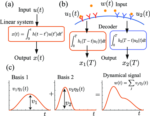
Figure 1: (a) Relation between input $u(t)$ and output $x(t)$ in a linear system through linear response function $h(t)$. (b) Decoding of dynamical patterns by two decoding systems. Input signal $w(t)$ is received by $N$ types of receptors, and the signal is processed by subsequent internal molecular decoders ($N=2$ in this figure). The linear response function of the $i$th decoder is given by $h_{i}(t)$. Each decoder outputs results by $x_{i}(T)$. (c) Dynamical pattern $w(t)$ as a sum of basis functions $\eta_{j}(t)$ at intensities $v_{j}$.

Figure 2: Basis sets for the $M=2$ case [solid and dashed lines denote $\eta_{1}(t)$ and $\eta_{2}(t)$, respectively]. (a) Slow and fast patterns (basis set A). (b) Constant and oscillation patterns (basis set B).

II Models

We consider a biochemical sensory system that reads out extracellular dynamical patterns by receptors, subsequently processes the signal via decoding networks, and finally reports the result as the concentration of output molecular species [Fig. 1(b)]. We assume that there exist $N$ decoding systems, each of which consists of receptors and a subsequent decoding network [$N=2$ for Fig. 1(b)]. In order to quantify the amount of transmitted information, we need to define the probability density on dynamical patterns. As each dynamical pattern has infinite dimensions, the definition of their probability density function is not trivial. We model a dynamical pattern $w(t)$ by a sum of basis functions after Ref. Gallager (1968):

$$w(t)=\sum_{j=1}^{M}v_{j}\eta_{j}(t),$$ (1)

where $M$ is the number of basis functions, $\boldsymbol{\eta}(t)=[\eta_{1}(t),...,\eta_{M}(t)]$ are basis functions, and $\boldsymbol{v}=[v_{1},...,v_{M}]$ are their coefficients, which are referred to as intensities. Figure 1(c) describes the model, where a dynamical pattern $w(t)$ is composed of two basis functions, $\eta_{1}(t)$ and $\eta_{2}(t)$. The basis functions need not be orthogonal. However, except for a particular case of $I^{\mathrm{dup}}$ considered later herein, the basis functions should be linearly independent. We define probability density $P(\boldsymbol{v})$ on $\boldsymbol{v}$, which are used to define the probability density of the dynamical patterns. Although Eq. (1) is introduced to incorporate the probability density on dynamical patterns, the basis functions $\eta_{j}(t)$ and their number $M$ have direct biological interpretations for some intercellular communication. Cells can decode multiplexed dynamical patterns Behar and Hoffmann (2010); Kubota et al. (2012); Purvis and Lahav (2012); Behar et al. (2013); Purvis and Lahav (2013); Sano et al. (2016), where the patterns can be broadly classified into two basic dynamics, fast pulsatile and slow transient patterns. Cells can read out amplitude information embedded in the two patterns. In this example, the number of basis functions is $M=2$, and $\eta_{1}(t)$ and $\eta_{2}(t)$ correspond to the fast and slow patterns.

We assume that $\eta_{j}(t)$ is in a steady state for $t<0$, where we define $\eta_{j}(t)=0$ for the steady state concentration (and hence $w(t)=0$ for $t<0$), and $w(t)$ starts to change at time $t=0$. Due to stochasticity, accompanied by, e.g., stochastic receptor-ligand binding, each decoder reads out a degraded pattern $u_{i}(t)$:

$$u_{i}(t)=w(t)+\xi_{i}(t),$$

where $\xi_{i}(t)$ is the input noise of the $i$th type of receptors, defined by $\left\langle\xi_{i}(t)\right\rangle=0$, and $\left\langle\xi_{i}(t)\xi_{i^{\prime}}(t^{\prime})\right\rangle=2D_{i}\delta_{ii^{\prime}}\delta(t-t^{\prime})$, where $D_{i}$ is the noise intensity. The noise intensity $D_{i}$ depends primarily on the number of $i$th-type receptors and the dissociation constant of the binding-unbinding reaction Wang et al. (2007). Moreover the dissociation constant has a temperature dependence via the van’t Hoff equation.

Next, we model the dynamics of the decoders. Let $x_{i}(t)$ be the output concentration of the $i$th decoder at time $t$, and, for $t<0$, we define $x_{i}(0)=0$. Note that $w(t)$ and $x_{i}(t)$ are concentrations relative to steady state and so can take negative values. In order to make analytic calculation possible, we consider a deterministic limit of decoders Govern and ten Wolde (2012); Becker et al. (2015). Decoders consist of biochemical reactions subject to intrinsic noise, the concentration dynamics of which can be described by stochastic processes. If we consider an infinitely large number of molecules while keeping the concentration constant, intrinsic noise vanishes and the stochastic processes reduce to deterministic differential equations, which is referred to as the deterministic limit. We assume that decoders output results after a finite time $t=T$ (for simplicity, we set the same time interval for each decoder), and so $\boldsymbol{x}(T)=[x_{1}(T),...,x_{N}(T)]$ contain information on the dynamical pattern. Suppose that the $i$th decoder is the single-layer linear decoder (linear birth-death process) given by

$$\dot{z}_{i}(t)=-\theta_{i}z_{i}+u_{i}(t),$$ (2)

where $z_{i}(t)$ is the concentration of molecular species in the $i$th decoder, and $\theta_{i}$ is the degradation rate. In this decoder, $z_{i}(t)$ directly reports the result, i.e., $x_{i}(T)=z_{i}(T)$. A similar model was proposed for decoding calcium oscillation Marhl et al. (2006). Because of the linearity of Eq. (2), the output at time $t$ is given by a convolution integral:

$$x_{i}(t)=\int_{0}^{t}h_{i}(t-t^{\prime})u_{i}(t^{\prime})dt^{\prime},$$ (3)

where $h_{i}(t)$ is the linear response function. For this single-layer and linear case, $h_{i}(t)=e^{-\theta_{i}t}$. Biochemical decoders are often composed of multiple layers, which can yield complex linear response functions $h_{i}(t)$ [cf. Eq. (13)] Govern and ten Wolde (2012); Hinczewski and Thirumalai (2014); Becker et al. (2015). For arbitrary linear response functions, the average at $t=T$ is $\mu_{x_{i}}=\left\langle x_{i}(T)\right\rangle=\int_{0}^{T}h_{i}(T-t^{\prime})w(t^{\prime})dt^{\prime}$, and the variance is $\sigma_{x_{i}}^{2}=2D_{i}\int_{0}^{T}h_{i}(t^{\prime})^{2}dt^{\prime}$ Gallager (1968) (see Appendix A). Although we used $x(T)$ as the output of the decoders in the present model, based on Eq. (3), $x(T)$ can also be regarded as the (weighted) time integration of some intermediate concentration.

Let $x_{i}^{T}=x_{i}(T)$, which is output of the $i$th decoder at time $t=T$. The amount of information contained in the output $\boldsymbol{x}^{T}=[x_{1}^{T},x_{2}^{T},...,x_{N}^{T}]$ is quantified by the mutual information

$$I[\boldsymbol{x}^{T};\boldsymbol{v}]=\int d\boldsymbol{x}^{T}\int d\boldsymbol{v}\,P(\boldsymbol{x}^{T}|\boldsymbol{v})P(\boldsymbol{v})\ln\left[\frac{P(\boldsymbol{x}^{T}|\boldsymbol{v})}{P(\boldsymbol{x}^{T})}\right].$$ (4)

Here, $P(\boldsymbol{x}^{T}|\boldsymbol{v})$ is the probability density of $\boldsymbol{x}^{T}$ given $\boldsymbol{v}$, and $P(\boldsymbol{v})$ is the probability density on $\boldsymbol{v}=[v_{1},..,v_{M}]$. Equation (4) is the quantity defined between $\boldsymbol{x}$ at time $t=T$ and $\boldsymbol{v}$. We assume independent probability densities for $v_{j}$, $P(\boldsymbol{v})=\prod_{j=1}^{M}P(v_{j})$, where $P(v_{j})$ is the Gaussian distribution with mean $0$ and variance $\sigma_{v_{j}}^{2}$. Although we assumed independence for $v_{j}$, we can eliminate this assumption when $\boldsymbol{v}$ is distributed according to a multivariate Gaussian distribution. If $\boldsymbol{v}$ has a multivariate Gaussian distribution, we can apply a linear transform to redefine basis functions $\boldsymbol{\eta}(t)$ so that elements of $\boldsymbol{v}$ become uncorrelated with each other (see Appendix B). Since uncorrelated Gaussian random variables are independent, we can always make the independence assumption for $\boldsymbol{v}$.

We wish to find optimal decoders which maximally extract information from dynamical patterns. Instead of exploring all possible candidate structures, we optimize a set of linear response functions $\boldsymbol{h}(t)=[h_{1}(t),...,h_{N}(t)]$ with the calculus of variations. Thus we obtain a desirable biochemical system through an optimization problem with an identifiable objective function Hasegawa and Arita (2014a, b); Hasegawa (2016).

Taking into account biological situations, we consider the following three optimization problems (italicized words in parentheses are abbreviations): (i) maximization of $I[\boldsymbol{x}^{T};\boldsymbol{v}]$ (full decoder), (ii) maximization of $I[\boldsymbol{x}^{T};\boldsymbol{v}]$ with $P(\boldsymbol{x}^{T})=\prod_{i}P(x_{i}^{T})$ (decorrelating decoder), and (iii) maximization of $I[\boldsymbol{x}^{T};\boldsymbol{v}]$ with single-layer linear decoders (SLL decoder). For (i), decoders obtained by full maximization provide an upper bound on the mutual information between dynamical patterns and output. When cells want to extract as much information as possible, this maximization is suitable. For (ii), $P(\boldsymbol{x}^{T})=\prod_{i}P(x_{i}^{T})$ can be easily incorporated into the maximization if $N=M$, which is assumed here. As the input noises $\boldsymbol{\xi}(t)=[\xi_{1}(t),...,\xi_{N}(t)]$ affect each receptor independently (Fig. 1(b)), we have $P(\boldsymbol{x}^{T}|\boldsymbol{v})=\prod_{i=1}^{N}P(x_{i}^{T}|\boldsymbol{v})$. Combining these relations, we arrive at

$$P(\boldsymbol{x}^{T}) =\int d\boldsymbol{v}\,P(\boldsymbol{x}^{T}|\boldsymbol{v})P(\boldsymbol{v}),$$

$$=\int d\boldsymbol{v}\,\prod_{i=1}^{N}P(x_{i}^{T}|\boldsymbol{v})\prod_{j=1}^{N(=M)}P(v_{j}).$$

If each $P(x_{i}^{T}|\boldsymbol{v})$ disjointly depends on only one $v_{i}$ [i.e., $P(x_{i}^{T}|\boldsymbol{v})=P(x_{i}^{T}|v_{i})$], we can show that $P(\boldsymbol{x}^{T})=\prod_{i}P(x_{i}^{T})$. This is similar to a decorrelator in digital communication, which decorrelates multiplexed signals (see Appendix C). For this case, $v_{i}$ can be obtained by measuring only one $x_{i}(T)$, i.e., $I[\boldsymbol{x}^{T};\boldsymbol{v}]=\sum_{i=1}^{N}I[x_{i}^{T};v_{i}]$. For (iii), we fix the linear response function to $h_{i}(t)=e^{-\theta_{i}t}$, which corresponds to the abovementioned single-layer linear (SLL) decoder. We optimize all $\theta_{i}$ numerically with simulated annealing to maximize $I[\boldsymbol{x}^{T};\boldsymbol{v}]$.

For arbitrary $N$ and $M$ (both $N=M$ and $N\neq M$ are allowed), we obtain the optimal linear response functions as follows (see Appendix C):

$$h_{i}(t)=-\frac{1}{4\Lambda_{i}D_{i}}\sum_{j=1}^{M}\lambda_{ij}\eta_{j}(T-t),$$ (5)

where $\lambda_{ij}$ and $\Lambda_{i}$ are Lagrange multipliers (real values), and these values depend on the type of decoders (full or decorrelating). When observing the dynamical pattern composed of a single basis function ($M=1$) with a single decoder ($N=1$), the optimal linear response function is $h_{1}(t)\propto\eta_{1}(T-t)$, which is known as the matched filter. From Eq. (5), the optimal linear response function that maximizes the mutual information is given by the summation of matched filters. Although the matched filter is known to be optimal for $M=N=1$, the optimality of Eq. (5) for maximization of the mutual information is not trivial.

III Results

III.1 Mutual information

We construct concrete optimal linear response functions for a system with $N=M=2$. In actual inter-cellular communication, as far as known, the degree of multiplexing is very small. Moreover, obtaining optimal linear response functions becomes more difficult as $N$ or $M$ increases. Therefore, we select $N=M=2$ as the minimal model for the multi-dimensional information processing. For the basis functions $\eta_{j}(t)$, we consider the two basis sets shown in Figs. 2(a) and (b). The two basis sets A and B are defined by

$$\mathrm{Set\,A}\begin{cases}\eta_{1}(t)&=\sqrt{\frac{2}{3}}(1-\cos(2\pi t)),\\ \eta_{2}(t)&=\frac{2}{\sqrt{3}}\Theta\left(\frac{1}{2}-t\right)(1-\cos(4\pi t)),\end{cases}$$ (6)

and

$$\mathrm{Set\,B}\begin{cases}\eta_{1}(t)&=1,\\ \eta_{2}(t)&=\sqrt{\frac{2}{3}}(1-\cos(4\pi t)).\end{cases}$$ (7)

Basis set A comprises slow and fast patterns (Fig. 2(a)), where $\Theta(t)$ is a step function; and basis set B comprises constant and oscillation patterns (Fig. 2(b)). All of the basis functions are normalized so that $\psi_{11}=1$ and $\psi_{22}=1$, where $\psi_{jj^{\prime}}$ is the correlation matrix defined by $\psi_{jj^{\prime}}=\int_{0}^{T}\eta_{j}(t)\eta_{j^{\prime}}(t)dt$. Regarding $T$, it is reasonable to choose $T$ as the largest duration time among $\eta_{j}(t)$. If $T$ is shorter than the largest time, decoders cannot use all of the information contained in $w(t)$. Conversely, even if $T$ is longer than the largest time, decoders cannot extract more information from $w(t)$. Therefore, we use $T=1$ for both of the basis sets.

Let $I^{\mathrm{full}}$, $I^{\mathrm{decor}}$, and $I^{\mathrm{sll}}$ be the mutual information $I[\boldsymbol{x}^{T};\boldsymbol{v}]$ of the full, decorrelating, and SLL decoders, respectively. $I^{\mathrm{full}}$, $I^{\mathrm{decor}}$, and $I^{\mathrm{sll}}$ are obtained by optimizing the linear response functions. As explained above, the mutual information quantities assume a model in which information is embedded in two linearly independent basis functions, is transmitted through a common channel, and is decoded by two decoders (Fig. 3(a)). We cannot obtain closed-form solutions for $I^{\mathrm{full}}$ and $I^{\mathrm{sll}}$ for arbitrary noise intensity, so we calculate the solutions numerically (see Appendix C). For sufficiently small $D_{1}$ and $D_{2}$, $I^{\mathrm{full}}$ is approximated by

$$I^{\mathrm{full}}\simeq\frac{1}{2}\ln\left(\frac{\sigma_{v_{1}}^{2}\sigma_{v_{2}}^{2}\left(\psi_{11}\psi_{22}-\psi_{12}^{2}\right)}{4D_{1}D_{2}}\right).$$ (8)

When $\eta_{1}(t)$ and $\eta_{2}(t)$ are linearly independent, we have $\psi_{11}\psi_{22}>\psi_{12}^{2}$. $I^{\mathrm{decor}}$ can be calculated in closed form for arbitrary noise intensity (see Appendix C). For sufficiently small $D_{1}$ and $D_{2}$, $I^{\mathrm{decor}}$ is approximated by

$$I^{\mathrm{decor}}\simeq\frac{1}{2}\ln\left(\frac{\sigma_{v_{1}}^{2}\sigma_{v_{2}}^{2}\left(\psi_{11}\psi_{22}-\psi_{12}^{2}\right)^{2}}{4D_{1}D_{2}\psi_{11}\psi_{22}}\right).$$ (9)

For comparison, we consider the mutual information $I^{\mathrm{dual}}$ which corresponds to a model where information embedded in two basis functions is transmitted through two designated channels and is decoded by two designated decoders (Fig. 3(b)). Applying the calculus of variations, $I^{\mathrm{dual}}$ is represented by

$$I^{\mathrm{dual}} =I[x_{1}^{T};v_{1}]+I[x_{2}^{T};v_{2}],$$

$$=\frac{1}{2}\ln\left(1+\frac{\sigma_{v_{1}}^{2}\psi_{11}}{2D_{1}}\right)+\frac{1}{2}\ln\left(1+\frac{\sigma_{v_{2}}^{2}\psi_{22}}{2D_{2}}\right).$$ (10)

Note that $I^{\mathrm{dual}}$ does not have biological relevance but is introduced merely as a theoretical reference point. From Eqs. (8) and (10), when $D_{1}$ and $D_{2}$ are sufficiently small, the following relation holds:

$$I^{\mathrm{full}}\leq I^{\mathrm{dual}},$$ (11)

where it holds with equality when the correlation between the two basis functions is zero (i.e., $\psi_{12}=0$).

Figures 4(a) and (b) show $I^{\mathrm{full}}$, $I^{\mathrm{decor}}$, $I^{\mathrm{sll}}$, and $I^{\mathrm{dual}}$ (solid, dashed, dotted, and dot-dashed lines, respectively) as functions of the noise intensity $D\ (=D_{1}=D_{2})$ for basis sets A and B, respectively. Parameter details are shown in the caption of Fig. 4. In Figs. 4(a) and (b), we see that $I^{\mathrm{full}}$ and $I^{\mathrm{decor}}$ yield higher values than $I^{\mathrm{sll}}$ for a lower noise intensity $D$, especially in Fig. 4(a), which indicates that optimal linear response functions extract information more efficiently than SLL decoders. The insets in Figs. 4(a) and (b) highlight $I^{\mathrm{dual}}-I^{\mathrm{full}}$ as a function of $D$. Interestingly, for large noise intensity $D$, the two mutual information quantities $I^{\mathrm{full}}$ and $I^{\mathrm{dual}}$ obey $I^{\mathrm{full}}>I^{\mathrm{dual}}$, which is the opposite relation to Eq. (11) (Eq. (11) is satisfied for sufficiently small $D$). This relation is nontrivial because the use of designated channels, which corresponds to $I^{\mathrm{dual}}$, is expected to provide higher information transmission, as shown by Eq. (11).

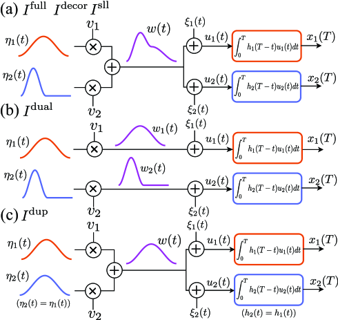
Figure 3: Information transmission model assumed in different mutual information. (a) Information is embedded in two distinct basis functions, transmitted through one common channel, and decoded by two decoders. (b) Information is embedded in two distinct basis functions, transmitted through two designated channels, and decoded by two decoders. (c) Information is embedded in two identical basis functions, transmitted through one channel, and decoded by two identical decoders. In (a)–(c), $\oplus$ and $\otimes$ denote addition and multiplication operations, respectively.

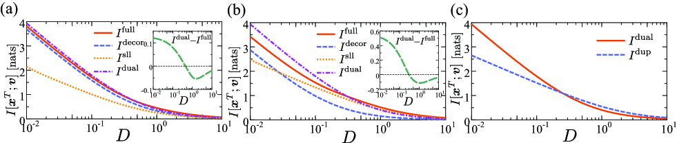
Figure 4: (a) and (b) Mutual information as a function of noise intensity $D$ by basis set; (a) basis set A [Fig. 2(a)] and (b) basis set B [Fig. 2(b)]. Solid, dashed, dotted, and dot-dashed lines denote $I^{\mathrm{full}}$, $I^{\mathrm{decor}}$, $I^{\mathrm{sll}}$, and $I^{\mathrm{dual}}$, respectively. In (a) and (b), the insets highlight $I^{\mathrm{dual}}-I^{\mathrm{full}}$ as a function of $D$. (c) Mutual information quantities $I^{\mathrm{dual}}$ (solid line) and $I^{\mathrm{dup}}$ (dashed line) as functions of $D$. Note that $I^{\mathrm{dual}}$ and $I^{\mathrm{dup}}$ do not depend on the basis set. In all panels, parameters are $T=1$ and $\sigma_{v_{1}}^{2}=\sigma_{v_{2}}^{2}=1$.

In order to investigate the cause of this opposite relation between $I^{\mathrm{full}}$ and $I^{\mathrm{dual}}$ with respect to $D$, we examine the optimal response functions, which are shown in Fig. 5. Figures 5(a) and (b) show linear response functions $h_{1}(t)$ (solid line) and $h_{2}(t)$ (dashed line) for the full decoder with basis set A for different noise intensities ($D=0.1$ and $1.0$, respectively) while keeping the other parameters unchanged (details are shown in the caption of Fig. 5). Note that for $D<0.1$, the shapes of the optimal linear response functions are similar to that of $D=0.1$, and for $D>1.0$, the shapes are similar to that of $D=1.0$. In Fig. 5(c), we also show the optimal linear response functions $h_{1}(t)$ (solid line) and $h_{2}(t)$ (dashed line) for the decorrelating decoder. In this case, there is no major difference when noise intensity $D$ is varied. We can see that for $D=0.1$ (Fig. 5(a)), the linear response function of the full decoder is similar to that of the decorrelating decoder of Fig. 5(c), indicating that the decorrelation can provide near-optimal efficiency for the weak-noise case. In Fig. 5(a), $h_{i}(t)$ indicated by solid and dashed lines mainly decode information embedded in slow and fast patterns, respectively. When we increase $D$ in the fully optimal case, the two linear response functions coalesce to a single function (the critical points are $D\simeq 0.83$ for basis set A and $D\simeq 0.20$ for basis set B). This result indicates that, when the noise intensity is very strong, decoding information with two distinct decoders is inefficient but decoding with identical decoders is relatively efficient. Therefore, in the region in which $I^{\mathrm{full}}$ and $I^{\mathrm{dual}}$ obey $I^{\mathrm{dual}}<I^{\mathrm{full}}$, a qualitative change in the linear response functions occurred.

In order to explain this change in great detail, we introduce another mutual information quantity $I^{\mathrm{dup}}$, which assumes a model similar to that shown in Fig. 3(a) but uses the same function for the two basis functions ($\eta_{1}(t)=\eta_{2}(t)$) and the same linear response function for the two decoders ($h_{1}(t)=h_{2}(t)$), as shown in Fig. 3(c). We also set $D_{1}=D_{2}=D$ and $\sigma_{v_{1}}^{2}=\sigma_{v_{2}}^{2}=\sigma_{v}^{2}$. Optimizing the linear response functions, $I^{\mathrm{dup}}$ is given by (see Appendix C)

$$I^{\mathrm{dup}} =\frac{1}{2}\ln\left(1+\frac{2\sigma_{v}^{2}\psi}{D}\right),$$ (12)

where $\psi=\psi_{11}=\psi_{22}$. Figure 4(c) shows $I^{\mathrm{dual}}$ and $I^{\mathrm{dup}}$ as functions of $D$, and we observe that $I^{\mathrm{dual}}>I^{\mathrm{dup}}$ for weaker noise intensity, while $I^{\mathrm{dup}}>I^{\mathrm{dual}}$ for larger noise intensity. This indicates that when the noise intensity is excessively large, multi-dimensional information transmission becomes inefficient. Transmitting information by embedding information into two identical basis functions and decoding using two identical decoders becomes more efficient.

Figure 5: (a) and (b) Optimal linear response function $h_{i}(t)$ of the full decoder with basis set A for different noise intensities; (a) $D=0.1$ and (b) $D=1.0$, where all other parameters are the same. (c) Optimal linear response function $h_{i}(t)$ of the decorrelating decoder with $D=0.1$. In all panels, the solid and dashed lines denote $h_{1}(t)$ and $h_{2}(t)$, respectively. For all $h_{i}(t)$ shown, the functionsthat are horizontally symmetric with respect to $h_{i}=0$ are also optimal solutions. We set $\sigma_{x_{1}}^{2}=\sigma_{x_{2}}^{2}=1$, and these parameters affect only the magnitude of the functions. The other parameters are identical to those in Fig. 4.

Figure 6: (a) Molecular realization of $h_{1}(t)$ in Fig. 5(a), and (b) its linear response function. In (a), arrows and bar-headed arrows denote activation and inhibition, respectively. In (b), the dashed line is the linear response function of the realization network and the solid line is the target optimal linear response function shown in Fig. 5(a). (c) Molecular realization of $h_{2}(t)$ in Fig. 5(a) and (d) its linear response function. (e) Reduced molecular realization for the full network shown in Fig. 6(a) and (f) its linear response function. In (c)–(f), the meanings of the arrows and lines are the same as in (a) and (b).

III.2 Biochemical implementation

We next explore a biochemical implementation of the optimal decoders. We attempt to implement a decoding network corresponding to $h_{i}(t)$ with $K_{i}$ molecular species ($K_{i}$ is determined by the degree of the transfer function; see below). Linearizing around the steady state, we describe their dynamics by the following linear model:

$$\dot{\boldsymbol{z}}_{i}(t)=\boldsymbol{A}_{i}\boldsymbol{z}_{i}(t)+\boldsymbol{b}_{i}u_{i}(t).$$ (13)

where $\boldsymbol{z}_{i}(t)=[z_{i1}(t),....,z_{iK_{i}}(t)]^{\top}$, $z_{ik}(t)$ is the relative concentration of the $k$th molecular species in the $i$th decoder, $\boldsymbol{A}_{i}$ is a $K_{i}\times K_{i}$ matrix, and $\boldsymbol{b}_{i}$ is a $K_{i}$-dimensional column vector. The output of Eq. (13) is $z_{iK_{i}}(t)$ and hence $x_{i}(T)=z_{iK_{i}}(T)$ (the last molecular species reports the result). Independent of the type of maximization (the full or decorrelating decoders), from Eq. (5), Laplace transform yields

$$\tilde{h}_{i}(s)=-\frac{1}{4\Lambda_{i}D_{i}}\sum_{j=1}^{M}\lambda_{ij}\tilde{\eta}_{j}(s),$$ (14)

where $\tilde{h}_{i}(s)=\mathcal{L}[h_{i}(t)]$ (the transfer function) and $\tilde{\eta}_{j}(s)=\mathcal{L}[\tilde{\eta}_{j}(T-t)]$ with $\mathcal{L}$ being the Laplace transform. We want to identify $\boldsymbol{A}_{i}$ and $\boldsymbol{b}_{i}$ which yield the desired transfer functions $\tilde{h}_{i}(s)$. This problem is known as the realization problem in control theory Williams and Lawrence (2007). Let the transfer function be a rational polynomial function of the form

$$\tilde{h}_{i}(s)=\frac{\sum_{k=1}^{K_{i}}\beta_{ik}s^{K_{i}-k}}{s^{K_{i}}+\sum_{k=1}^{K_{i}}\alpha_{ik}s^{K_{i}-k}},$$ (15)

where $\beta_{ik}$ and $\alpha_{ik}$ are real values, and the degree of the denominator is larger than that of the nominator (this condition is called strictly proper). From control theory, one possible realization of this transfer function is (see Appendix D)

$$\boldsymbol{A}_{i}=\left[\begin{array}[]{ccccc}0&0&0&\cdots&-\alpha_{iK_{i}}\\ 1&0&0&\cdots&-\alpha_{i,K_{i}-1}\\ 0&1&0&\cdots&-\alpha_{i,K_{i}-2}\\ \vdots&\vdots&\vdots&\ddots&\vdots\\ 0&0&0&1&-\alpha_{i1}\end{array}\right],\boldsymbol{b}_{i}=\left[\begin{array}[]{c}\beta_{iK_{i}}\\ \beta_{i,K_{i}-1}\\ \beta_{i,K_{i}-2}\\ \vdots\\ \beta_{i1}\end{array}\right].$$ (16)

Off-diagonal ones in Eq. (16) imply that $z_{ik}$ depends on $z_{i,k-1}$ ($k=2,3,...,K_{i}$), which corresponds to a cascade topology. When the transfer function is strictly proper, its corresponding linear systems can be implemented by a cascade network with additional feedback and feedforward loops. As is well known, the cascade topology is prevalent in actual signaling networks and additional feedback and feedforward loops exists in the networks, implying that it is possible to implement optimal decoders biochemically.

As an example, we construct biochemical implementations for the decoders of the basis set A with $D=0.1$ (Fig. 5(a)). We show the biochemical networks in Figs. 6(a) and (c), which are realizations of $h_{1}(t)$ and $h_{2}(t)$ in Fig. 5(a), respectively. Figures 6(b) and (d) show linear response functions of the networks in Figs. 6(a) and (c), respectively. The realization networks are created by applying the Fourier series expansion to $\eta_{j}(t)$ and calculating their Laplace transform (see Appendix D). In Figs. 6(a) and (c), when matrix elements of $\boldsymbol{A}_{i}$ and $\boldsymbol{b}_{i}$ are positive or negative, we display their relation by activation (arrow) or inhibition (bar-headed arrow), respectively. In Figs. 6(b) and (d), we can see that the linear response functions of the molecular networks (dashed line) are indistinguishable from the target optimal linear response function $h_{i}(t)$ (solid line). This indicates that the biochemical networks which maximally exploit information from dynamical patterns can be implemented. The network in Fig. 6(c) decodes the fast pattern, while that in Fig. 6(a) decodes the slow pattern. The main difference between these two networks is that the latter has an incoherent feed-forward loop (iFFL) Mangan and Alon (2003); Alon (2007), while the former does not. Reference Noguchi et al. (2013) indicated that, when decoding temporal insulin patterns, a decoding network having an iFFL is responsive against a fast pulsatile pattern, while it does not respond to a slow ramp pattern. Because transfer functions $\tilde{h}_{1}(s)$ and $\tilde{h}_{2}(s)$ are sums of $\tilde{\eta}_{1}(s)$ and $\tilde{\eta}_{2}(s)$ with different weighting, they are rational polynomial functions with the same denominator unless they can be reduced. If $\tilde{h}_{1}(s)$ and $\tilde{h}_{2}(s)$ have the same denominator, $\boldsymbol{A}_{1}$ and $\boldsymbol{A}_{2}$ of these realizations become identical (cf. Eqs. (15) and (16)) and this is a reason why the realization networks of Figs. 6(a) and (c) have the same feedback structure from the output. Both of the implementations have 7 nodes (i.e., $K_{1}=K_{2}=7$). However, we note that the molecular networks can be minimized without losing much of their response. Specifically, we construct a reduced realization network for the full network shown in Fig. 6(a). Figures 6(e) and (f) show the reduced network, which consists of 3 nodes ($K_{1}=3$), and its corresponding linear response function, respectively. The meanings of the arrows in Fig. 6(e) and the lines in Fig. 6(f) are identical to those in Figs. 6(a) and (b), respectively. From Fig. 6(f), we see that the response of the reduced realization network (dashed line) is similar to that of the optimal realization network (solid line). Although the number of nodes in the reduced network (Fig. 6(e)) is smaller than in the corresponding full network (Fig. 6(a)), the basic structures are similar: there are positive feedforward loops from the input and negative feedback loops from the output, and there is no iFFL (see Appendix D). We constructed this reduced network heuristically based on the balanced truncation in control theory. It is worthwhile to develop a systematic reduction procedure, which would lead to feasible biochemical implementations.

IV Concluding Remarks

In this manuscript, we considered the optimal decoding of dynamical patterns through maximization of mutual information between input and output. We found that when the noise intensity is relatively low, the distinct decoders can extract much information, as expected. On the other hand, when the noise intensity is very high, distinct decoders cannot achieve the optimal extraction of the information, while identical decoders can. Although multiplexing is naturally considered to confer higher information transmission, our results show that this is not necessarily true for the case in which receptors are subject to strong noise. Still, we note that when decoding information with the identical decoders, it is impossible to demultiplex dynamical signals. Therefore, the decoders can determine the intensity of $v_{1}$ or $v_{2}$ but cannot identify whether the intensity corresponds to $v_{1}$ or $v_{2}$. As indicated by several experiments, cells use multiplexed dynamical patterns to transmit information. If the primary goal of cellular sensory networks is transmitting as much information as possible, our results can provide insight into a possible range of the noise intensity. Furthermore, we investigated the possibility of biochemical implementation of the optimal decoders and found that such optimal decoders can be implemented by a modification of the cascade network.

Recently, extensive research has been conducted in order to construct relations between thermodynamic cost and mutual information Parrondo et al. (2015), especially in biological contexts Sartori et al. (2014); Barato et al. (2014). In particular, Ref. Ouldridge et al. (2017) studied the thermodynamic cost of the mutual information between receptors and readouts using a Markov process. Our model considers the deterministic limit and hence it ignores the intrinsic thermal noise. When we incorporate the effect of intrinsic noise, the mutual information between patterns and output should be bounded above by some thermodynamic cost. Exploration of this topic is left for future research.

Appendix A Mean and variance of output

We calculate the mean and the variance of output of the $i$th decoder as follows. As described in the main text, we can express the output of the $i$th decoder by Eq. (3). The mean at time $t=T$ is

$$\mu_{x_{i}} =\left\langle x_{i}(T)\right\rangle,$$

$$=\int_{0}^{T}h_{i}(T-t^{\prime})\left\langle w(t^{\prime})+\xi_{i}(t^{\prime})\right\rangle dt^{\prime},$$

$$=\int_{0}^{T}h_{i}(T-t^{\prime})w(t^{\prime})dt^{\prime},$$

$$=\sum_{j=1}^{M}v_{j}q_{ij},$$ (17)

where we define

$$q_{ij}=\int_{0}^{T}h_{i}(T-t^{\prime})\eta_{j}(t^{\prime})dt^{\prime}.$$ (18)

Similarly, the variance at time $t=T$ is given by

$$\sigma_{x_{i}}^{2} =\left\langle x_{i}(T)^{2}\right\rangle-\left\langle x_{i}(T)\right\rangle^{2},$$

$$=\int_{0}^{T}dt^{\prime}\int_{0}^{T}dt^{\prime\prime}\,h_{i}(T-t^{\prime})h_{i}(T-t^{\prime\prime})\left\langle\xi_{i}(t^{\prime})\xi_{i}(t^{\prime\prime})\right\rangle,$$

$$=2D_{i}\int_{0}^{T}h_{i}(t^{\prime})^{2}dt^{\prime}.$$ (19)

Appendix B Independence of $\boldsymbol{v}$

We can make elements in $\boldsymbol{v}=[v_{1},...,v_{M}]$ independent of each other through a change of basis functions $\boldsymbol{\eta}(t)=[\eta_{1}(t),...,\eta_{M}(t)]$. We define a covariance matrix $\boldsymbol{\mathcal{C}}=\left\langle\boldsymbol{v}^{\top}\boldsymbol{v}\right\rangle$, the elements of which are

$$\mathcal{C}_{ij}=\left\langle v_{i}v_{j}\right\rangle=\int v_{i}v_{j}P(v_{i},v_{j})dv_{i}dv_{j},$$

where we assumed $\left\langle v_{j}\right\rangle=0$. Because the covariance matrix $\boldsymbol{\mathcal{C}}$ is real symmetric, it can be diagonalized by an orthogonal matrix $\boldsymbol{\mathcal{Q}}$:

$$\boldsymbol{\mathcal{D}}=\mathcal{\boldsymbol{\mathcal{Q}}}^{\top}\boldsymbol{\mathcal{C}}\mathcal{\boldsymbol{\mathcal{Q}}},$$

where $\boldsymbol{\mathcal{D}}$ is a diagonal matrix (diagonal elements are eigenvalues of $\boldsymbol{\mathcal{C}}$). Considering a change of basis functions $\boldsymbol{\eta}^{\prime}(t)^{\top}=\boldsymbol{\mathcal{Q}}^{\top}\boldsymbol{\eta}(t)^{\top}$, a new coefficient vector $\boldsymbol{v}^{\prime\top}=\mathcal{\boldsymbol{\mathcal{Q}}}^{\top}\boldsymbol{v}^{\top}$ has a diagonal covariance matrix:

$$\left\langle\boldsymbol{v}^{\prime\top}\boldsymbol{v}^{\prime}\right\rangle=\left\langle\mathcal{\boldsymbol{\mathcal{Q}}}^{\top}\boldsymbol{v}^{\top}\boldsymbol{v}\mathcal{\boldsymbol{\mathcal{Q}}}\right\rangle=\mathcal{\boldsymbol{\mathcal{Q}}}^{\top}\boldsymbol{\mathcal{C}}\mathcal{\boldsymbol{\mathcal{Q}}}=\boldsymbol{\mathcal{D}},$$

showing that elements in $\boldsymbol{v}^{\prime}$ are decorrelated. When $\boldsymbol{v}$ obeys the multivariate Gaussian distribution, elements in $\boldsymbol{v}^{\prime}$ are independent of each other. Note that we cannot make arbitrary random variables independent of each other by a change of basis functions.

Appendix C Optimal linear response function

According to the Gaussian assumption of probability density of $x_{i}^{T}$ ($x_{i}$ at time $t=T$), we have

$$P(x_{i}^{T}|\boldsymbol{v})=\frac{1}{\sqrt{2\pi\sigma_{x_{i}}^{2}}}\exp\left(-\frac{\left(x_{i}^{T}-\sum_{j=1}^{M}v_{j}q_{ij}\right)^{2}}{2\sigma_{x_{i}}^{2}}\right).$$ (20)

As assumed in the main text, the probability distribution of $v_{j}$ is given by

$$P(v_{j})=\frac{1}{\sqrt{2\pi\sigma_{v_{j}}^{2}}}\exp\left(-\frac{v_{j}^{2}}{2\sigma_{v_{j}}^{2}}\right).$$ (21)

The mutual information is defined by Eq. (4). For $N=M=2$ which is considered in the manuscript, with Eqs. (20) and (21), the mutual information $I[\boldsymbol{x}^{T};\boldsymbol{v}]$ is given by:

$$I[x_{1}^{T},x_{2}^{T};v_{1},v_{2}]=\frac{1}{2}\ln\left[1+\frac{q_{11}^{2}\sigma_{v_{1}}^{2}+q_{12}^{2}\sigma_{v_{2}}^{2}}{\sigma_{x_{1}}^{2}}+\frac{q_{21}^{2}\sigma_{v_{1}}^{2}+q_{22}^{2}\sigma_{v_{2}}^{2}}{\sigma_{x_{2}}^{2}}+\frac{\sigma_{v_{1}}^{2}\sigma_{v_{2}}^{2}(q_{11}q_{22}-q_{12}q_{21})^{2}}{\sigma_{x_{1}}^{2}\sigma_{x_{2}}^{2}}\right].$$ (22)

We calculate optimal linear response function $h_{i}(t)$ which maximizes the mutual information $I[\boldsymbol{x}^{T};\boldsymbol{v}]$. As can be seen with Eq. (22), the mutual information $I[\boldsymbol{x}^{T};\boldsymbol{v}]$ is a function of $\boldsymbol{q}=[q_{ij}]$. Instead of directly maximizing $I[\boldsymbol{x}^{T};\boldsymbol{v}]$, we consider a more tractable function $\mathcal{M}(\boldsymbol{q})$ which satisfies the following condition:

$$\underset{\boldsymbol{q}}{\mathrm{argmax}}\,I[\boldsymbol{x}^{T};\boldsymbol{v}]=\underset{\boldsymbol{q}}{\mathrm{argmax}}\,\mathcal{M}(\boldsymbol{q}).$$

Then we consider the following performance index $\mathcal{R}(\boldsymbol{q},\boldsymbol{h})$:

$$\mathcal{R}(\boldsymbol{q},\boldsymbol{h}) =\mathcal{M}(\boldsymbol{q})+\sum_{i,j}\lambda_{ij}\left(q_{ij}-\int_{0}^{T}h_{i}(T-t)\eta_{j}(t)dt\right)$$

$$+\sum_{i}\Lambda_{i}\left(\sigma_{x_{i}}^{2}-2D_{i}\int_{0}^{T}h_{i}(t)^{2}dt\right),$$ (23)

where $\lambda_{ij}$ and $\Lambda_{i}$ are the Lagrange multipliers. Note that arguments of $\boldsymbol{q}$ in Eq. (23) are scalars while $\boldsymbol{h}$ are functions. Constraints corresponding to $\lambda_{ij}$ and $\Lambda_{i}$ are derived from Eqs. (18) and (19), respectively. Because $I[\boldsymbol{x}^{T};\boldsymbol{v}]$ is scale-invariant with respect to $h_{i}(t)$ and hence $\sigma_{x_{i}}$ does not affect the mutual information, we set $\sigma_{x_{i}}$ as constant (we set $\sigma_{x_{i}}=1$ for all $i$ in the main text). The total derivative of $\mathcal{R}(\boldsymbol{q},\boldsymbol{h})$ is written by

$$d\mathcal{R} =\sum_{i,j}\frac{\partial\mathcal{M}(\boldsymbol{q})}{\partial q_{ij}}dq_{ij}$$

$$+\sum_{i,j}\lambda_{ij}\left(dq_{ij}-\int_{0}^{T}\delta h_{i}(t)\eta_{j}(T-t)dt\right)$$

$$+\sum_{i}\Lambda_{i}\left(-4D_{i}\int_{0}^{T}h_{i}(t)\delta h_{i}(t)dt\right),$$

$$=\sum_{i,j}\left(\frac{\partial\mathcal{M}(\boldsymbol{q})}{\partial q_{ij}}+\lambda_{ij}\right)dq_{ij}$$

$$+\sum_{i}\int_{0}^{T}\delta h_{i}(t)\left(-\sum_{j}\lambda_{ij}\eta_{j}(T-t)-4D_{i}\Lambda_{i}h_{i}(t)\right)dt.$$ (24)

Because, $d\mathcal{R}$ should vanish at a stationary point, we obtain the following relations:

$$\frac{\partial\mathcal{M}(\boldsymbol{q})}{\partial q_{ij}}+\lambda_{ij} =0,$$ (25)

$$-\sum_{j}\lambda_{ij}\eta_{j}(T-t)-4D_{i}\Lambda_{i}h_{i}(t) =0.$$ (26)

From Eq. (26), we obtain

$$h_{i}(t)=-\frac{1}{4\Lambda_{i}D_{i}}\sum_{j=1}^{M}\lambda_{ij}\eta_{j}(T-t),$$ (27)

which is Eq. (5). Depending on the type of decoders (full or decorrelating), $\lambda_{ij}$ and $\Lambda_{i}$ are determined (see below). Substituting Eq. (27) into Eqs. (18) and (19), we have

$$q_{ij} =-\frac{1}{4\Lambda_{i}D_{i}}\sum_{k}\lambda_{ik}\psi_{kj},$$ (28)

$$\sigma_{x_{i}}^{2} =\frac{1}{8\Lambda_{i}^{2}D_{i}}\sum_{j,k}\lambda_{ij}\lambda_{ik}\psi_{kj},$$ (29)

where $[\psi_{jj^{\prime}}]$ is a correlation matrix of the basis functions $\eta_{j}(t)$, defined by

$$\psi_{jj^{\prime}}=\int_{0}^{T}\eta_{j}(t)\eta_{j^{\prime}}(t)dt.$$

Algebraic equations (25), (28), and (29) are solved with respect to $\boldsymbol{q}$, $\boldsymbol{\lambda}$, and $\boldsymbol{\Lambda}$ to obtain the maximum of $I[\boldsymbol{x};\boldsymbol{v}]$.

C.1 Full decoder

According to Eq. (22), we can use the following function for the full decoder:

$$\mathcal{M}(\boldsymbol{q}) =\frac{q_{11}^{2}\sigma_{v_{1}}^{2}+q_{12}^{2}\sigma_{v_{2}}^{2}}{\sigma_{x_{1}}^{2}}+\frac{q_{21}^{2}\sigma_{v_{1}}^{2}+q_{22}^{2}\sigma_{v_{2}}^{2}}{\sigma_{x_{2}}^{2}}$$

$$+\frac{\sigma_{v_{1}}^{2}\sigma_{v_{2}}^{2}(q_{11}q_{22}-q_{12}q_{21})^{2}}{\sigma_{x_{1}}^{2}\sigma_{x_{2}}^{2}},$$ (30)

Because it is difficult to obtain closed-form solutions for Eqs. (25), (28), and (29) along with Eq. (30), we numerically solve the equations.

When the noise intensity $D_{i}$ is sufficiently weak, we find the following expression:

$$I^{\mathrm{full}} \simeq\frac{1}{2}\ln\left[\frac{\sigma_{v_{1}}^{2}\sigma_{v_{2}}^{2}(q_{11}q_{22}-q_{12}q_{21})^{2}}{\sigma_{x_{1}}^{2}\sigma_{x_{2}}^{2}}\right],$$

$$=\frac{1}{2}\ln\left[\frac{\sigma_{v_{1}}^{2}\sigma_{v_{2}}^{2}\left(\psi_{11}\psi_{22}-\psi_{12}^{2}\right)}{4D_{1}D_{2}}\right],$$

which is Eq. (8) in the main text.

C.2 Decorrelating decoder

For $N=M(=2)$, which is considered in the manuscript, decorrelation is easily implemented. The output of the $i$th decoder at time $t=T$ is denoted by $x_{i}^{T}$ and its probability density is $P(x_{i}^{T}|\boldsymbol{v})$ (Eq. (20)). The relation can be represented by the Bayesian network shown in Fig. 7(a). For this case, the output probability density is not decorrelated, i.e., $P(\boldsymbol{x}^{T})\neq\prod_{i}P(x_{i}^{T})$ (note that since $P(\boldsymbol{x}^{T})$ is the Gaussian distribution, decorrelation is equivalent to independence). When $P(x_{i}^{T}|\boldsymbol{v})$ disjointly depends on only one $v_{j}\in\boldsymbol{v}$ as shown in Fig. 7(b), the output probability density is decorrelated. This condition yields $q_{ij}=0$ for $i\neq j$. We can use the following function for the decorrelating decoder:

$$\mathcal{M}(\boldsymbol{q})=\frac{q_{11}^{2}\sigma_{v_{1}}^{2}}{\sigma_{x_{1}}^{2}}+\frac{q_{22}^{2}\sigma_{v_{2}}^{2}}{\sigma_{x_{2}}^{2}}+\frac{\sigma_{v_{1}}^{2}\sigma_{v_{2}}^{2}q_{11}^{2}q_{22}^{2}}{\sigma_{x_{1}}^{2}\sigma_{x_{2}}^{2}}.$$ (31)

We obtain the mutual information as follows:

$$I^{\mathrm{decor}} =\frac{1}{2}\ln\left[1+\frac{\left(\psi_{11}\psi_{22}-\psi_{12}^{2}\right)\left(2D_{1}\psi_{22}\sigma_{v_{2}}^{2}+2D_{2}\psi_{11}\sigma_{v_{1}}^{2}+\left(\psi_{22}\psi_{11}-\psi_{12}^{2}\right)\sigma_{v_{1}}^{2}\sigma_{v_{2}}^{2}\right)}{4D_{1}D_{2}\psi_{11}\psi_{22}}\right].$$ (32)

When the noise intensity $D_{i}$ is sufficiently weak, the mutual information reduces to Eq. (9).

C.3 Calculation of $I^{\mathrm{dup}}$

Because $\eta_{1}(t)=\eta_{2}(t)=\eta(t)$ and $h_{1}(t)=h_{2}(t)=h(t)$ in $I^{\mathrm{dup}}$, $q_{ij}$ and $\sigma_{x_{i}}^{2}$ do not depend on $i$ or $j$, where we define $q_{ij}=q$ and $\sigma_{x_{i}}^{2}=\sigma_{x}^{2}$, respectively. Therefore, from Eq. (22), the mutual information is

$$I[x_{1}^{T},x_{2}^{T};v_{1},v_{2}]=\frac{1}{2}\ln\left(1+\frac{4\sigma_{v}^{2}}{\sigma_{x}^{2}}q^{2}\right).$$

Because $h(t)\propto\eta(T-t)$ from Eq. (27), we have $q^{2}=\psi\sigma_{x}^{2}/(2D)$ and obtain Eq. (12).

Appendix D Network realization of transfer function

Figure 7: (a) and (b) Network representations of (a) $P(x_{i}^{T}|\boldsymbol{v})$ and (b) $P(x_{i}^{T}|v_{i})$ for $N=M$. (c) Basis function $\eta_{2}(t)$ of basis set A [Fig. 2(a)] (solid line) and its Fourier series approximation (dashed line).

In the main text, we explore biochemical realization of optimal linear response functions $h_{i}(t)$. We consider a general $K$-dimensional linear system:

$$\dot{\boldsymbol{z}}(t)=\boldsymbol{A}\boldsymbol{z}(t)+\boldsymbol{b}u(t),\hskip 10.00002pty(t)=\boldsymbol{c}\boldsymbol{z}(t),$$ (33)

where $\boldsymbol{z}(t)$ is a $K$-dimensional column vector, $y(t)$ is an output scalar variable, $\boldsymbol{A}$ is a $K\times K$ matrix, $\boldsymbol{b}$ is a $K$-dimensional column vector, and $\boldsymbol{c}$ is a $K$-dimensional row vector. Here we dropped subscripts that identify the decoder number in order to simplify the notation (e.g., $\boldsymbol{A}_{i}$ in the main text is simply expressed $\boldsymbol{A}$ here) because we are describing a general theory. It is known that the transfer function $\tilde{h}(s)$ of the linear system of Eq. (33) is given by

$$\tilde{h}(s)=\boldsymbol{c}(s\boldsymbol{I}-\boldsymbol{A})^{-1}\boldsymbol{b}=\sum_{i=0}^{\infty}\frac{1}{s^{i+1}}\boldsymbol{c}\boldsymbol{A}^{i}\boldsymbol{b},$$

where $\boldsymbol{I}$ is the identity matrix. Since the transfer function depends only on $\boldsymbol{c}\boldsymbol{A}^{i}\boldsymbol{b}$, the transfer function is invariant under coordinate transform $\boldsymbol{\boldsymbol{z}}^{\prime}=\mathcal{T}\boldsymbol{z}$, where $\mathcal{T}$ is a regular matrix. According to the Faddeev method, $(s\boldsymbol{I}-\boldsymbol{A})^{-1}$ can be calculated by the following formula:

$$(s\boldsymbol{I}-\boldsymbol{A})^{-1} =\frac{\boldsymbol{F}_{1}s^{K-1}+\cdots+\boldsymbol{F}_{K-1}s+\boldsymbol{F}_{K}}{s^{K}+f_{1}s^{K-1}+\cdots+f_{K-1}s+f_{K}},$$ (34)

where $\boldsymbol{F}_{i}$ and $f_{i}$ are defined as follows:

$$\boldsymbol{F}_{1} =\boldsymbol{I},\hskip 10.00002ptf_{1}=-\mathrm{tr}\boldsymbol{A},$$ (35)

$$\boldsymbol{F}_{i} =\boldsymbol{A}\boldsymbol{F}_{i-1}+f_{i-1}\boldsymbol{I},\hskip 10.00002ptf_{i}=-\frac{1}{i}\mathrm{tr}(\boldsymbol{A}\boldsymbol{F}_{i}).$$ (36)

We consider the following rational polynomial transfer function:

$$\tilde{h}(s)=\frac{\beta_{1}s^{K-1}+\cdots+\beta_{K-1}s+\beta_{K}}{s^{K}+\alpha_{1}s^{K-1}+\cdots+\alpha_{K-1}s+\alpha_{K}},$$ (37)

where $\alpha_{i}$ and $\beta_{i}$ are real coefficients. One possible realization of the transfer function of Eq. (37) in the form of Eq. (33) is

$$\boldsymbol{A}=\left[\begin{array}[]{ccccc}0&0&0&\cdots&-\alpha_{K}\\ 1&0&0&\cdots&-\alpha_{K-1}\\ 0&1&0&\cdots&-\alpha_{K-2}\\ \vdots&\vdots&\vdots&\ddots&\vdots\\ 0&0&0&1&-\alpha_{1}\end{array}\right],\hskip 10.00002pt\boldsymbol{b}=\left[\begin{array}[]{c}\beta_{K}\\ \beta_{K-1}\\ \beta_{K-2}\\ \vdots\\ \beta_{1}\end{array}\right],$$ (38)

and $\boldsymbol{c}=[\begin{array}[]{ccccc}0&0&\cdots&0&1\end{array}]$, which is known as the observer canonical form. Because of $\boldsymbol{c}$ in Eq. (38), the output is given by the last variable $y(t)=z_{K}(t)$.

In the main text, we consider network realization for basis set A, whose basis functions are given in Eq. (6). Since the step function yields a transfer function that does not fit into the form of Eq. (37), we apply the Fourier series expansion to $\eta_{2}(t)$ to obtain

$$\eta_{2}(t)=\frac{16\sin(2\pi t)}{3\sqrt{3}\pi}-\frac{16\sin(6\pi t)}{15\sqrt{3}\pi}-\frac{\cos(4\pi t)}{\sqrt{3}}+\frac{1}{\sqrt{3}}.$$

In Fig. 7(c), we compare $\eta_{2}(t)$ of the exact function (solid line) with the Fourier approximation (dashed line). The Laplace transforms of $\eta_{j}(T-t)$ are given by

$$\tilde{\eta}_{1}(s) =\mathcal{L}[\eta_{1}(T-t)]=\sqrt{\frac{2}{3}}\frac{1}{s}-\sqrt{\frac{2}{3}}\frac{s}{s^{2}+4\pi^{2}},$$

$$\tilde{\eta}_{2}(s) =\mathcal{L}[\eta_{2}(T-t)]=-\frac{s}{\sqrt{3}\left(s^{2}+16\pi^{2}\right)}-\frac{32}{3\sqrt{3}\left(s^{2}+4\pi^{2}\right)}$$

$$+\frac{32}{5\sqrt{3}\left(s^{2}+36\pi^{2}\right)}+\frac{1}{\sqrt{3}s},$$

where $\mathcal{L}$ is the Laplace transform operator. From Eq. (5), the Laplace transform of optimal linear response function $h_{i}(t)$ (i.e., the transfer function) is given by Eq. (14). $\tilde{h}_{i}(s)$ of Eq. (14) fits into the form of Eq. (37) since $\Lambda_{i}$ and $\lambda_{ij}$ are real values.

We next show explicit representations of $\boldsymbol{A}$ and $\boldsymbol{b}$ which are realizations of optimal linear response functions $h_{i}(t)$ ($h_{1}(t)$ and $h_{2}(t)$ in Fig. 5(a)). We use $\boldsymbol{A}_{i}$ and $\boldsymbol{b}_{i}$ to represent $\boldsymbol{A}$ and $\boldsymbol{b}$ of the $i$th decoder:

$$\boldsymbol{A}_{1} =\left[\begin{array}[]{ccccccc}0.0&0.0&0.0&0.0&0.0&0.0&0.0\\ 10.0&0.0&0.0&0.0&0.0&0.0&-22.15\\ 0.0&10.0&0.0&0.0&0.0&0.0&0.0\\ 0.0&0.0&10.0&0.0&0.0&0.0&-76.37\\ 0.0&0.0&0.0&10.0&0.0&0.0&0.0\\ 0.0&0.0&0.0&0.0&10.0&0.0&-55.27\\ 0.0&0.0&0.0&0.0&0.0&10.0&0.0\end{array}\right],$$ (46)

$$\boldsymbol{b}_{1} =\left[\begin{array}[]{ccccccc}3.78&1.50&2.32&1.13&0.35&0.11&0.0\end{array}\right]^{\top},$$ (48)

$$\boldsymbol{A}_{2} =\left[\begin{array}[]{ccccccc}0.0&0.0&0.0&0.0&0.0&0.0&0.0\\ 10.0&0.0&0.0&0.0&0.0&0.0&-22.15\\ 0.0&10.0&0.0&0.0&0.0&0.0&0.0\\ 0.0&0.0&10.0&0.0&0.0&0.0&-76.37\\ 0.0&0.0&0.0&10.0&0.0&0.0&0.0\\ 0.0&0.0&0.0&0.0&10.0&0.0&-55.27\\ 0.0&0.0&0.0&0.0&0.0&10.0&0.0\end{array}\right],$$ (56)

$$\boldsymbol{b}_{2} =\left[\begin{array}[]{ccccccc}2.25&-7.80&7.93&-5.88&2.05&-0.60&0.0\end{array}\right]^{\top}.$$ (58)

As denoted above, these realizations are not unique, as any coordinate transformation yields the same transfer function. Thus we applied some scaling matrix to adjust excessively large values in Eqs. (46)–(58), which seem to be biologically infeasible. We constructed a reduced realization for the full network of Fig. 6(a). $\boldsymbol{A}_{1}^{\prime}$ and $\boldsymbol{b}_{1}^{\prime}$, which are $\boldsymbol{A}$ and $\boldsymbol{b}$ of the reduced network, are given by

$$\boldsymbol{A}_{1}^{\prime} =\left[\begin{array}[]{ccc}0&0&0\\ 1.0&0&-39.50\\ 0&1.0&0\end{array}\right],$$ (62)

$$\boldsymbol{b}_{1}^{\prime} =\left[\begin{array}[]{ccc}67.40&2.52&0\end{array}^{\top}\right].$$ (64)

Network representations of Eqs. (46)–(64) are shown in Figs. 6(a), (c), and (e) in the main text, where positive and negative elements in $\boldsymbol{A}$ and $\boldsymbol{b}$ are described by activation (arrow) and inhibition (bar-headed arrow), respectively.

References

- Behar and Hoffmann (2010) M. Behar and A. Hoffmann, Curr. Opin. Genetics Dev. 20, 684 (2010).
- Purvis and Lahav (2013) J. E. Purvis and G. Lahav, Cell 152, 945 (2013).
- Kobayashi (2010) T. J. Kobayashi, Phys. Rev. Lett. 104, 228104 (2010).
- Hinczewski and Thirumalai (2014) M. Hinczewski and D. Thirumalai, Phys. Rev. X 4, 041017 (2014).
- Becker et al. (2015) N. B. Becker, A. Mugler, and P. R. ten Wolde, Phys. Rev. Lett. 115, 258103 (2015).
- Kubota et al. (2012) H. Kubota, R. Noguchi, Y. Toyoshima, Y.-i. Ozaki, S. Uda, K. Watanabe, W. Ogawa, and S. Kuroda, Mol. Cell 46, 820 (2012).
- Noguchi et al. (2013) R. Noguchi, H. Kubota, K. Yugi, Y. Toyoshima, Y. Komori, T. Soga, and S. Kuroda, Mol. Syst. Biol. 9, 664 (2013).
- Sano et al. (2016) T. Sano, K. Kawata, S. Ohno, K. Yugi, H. Kakuda, H. Kubota, S. Uda, M. Fujii, K. Kunida, D. Hoshino, et al., Sci. Signal. 9, ra112 (2016).
- Selimkhanov et al. (2014) J. Selimkhanov, B. Taylor, J. Yao, A. Pilko, J. Albeck, A. Hoffmann, L. Tsimring, and R. Wollman, Science 346, 1370 (2014).
- Tostevin and ten Wolde (2009) F. Tostevin and P. R. ten Wolde, Phys. Rev. Lett. 102, 218101 (2009).
- Mora and Wingreen (2010) T. Mora and N. S. Wingreen, Phys. Rev. Lett. 104, 248101 (2010).
- Mugler et al. (2010) A. Mugler, A. M. Walczak, and C. H. Wiggins, Phys. Rev. Lett. 105, 058101 (2010).
- Purvis and Lahav (2012) J. E. Purvis and G. Lahav, Mol. Cell 46, 715 (2012).
- Hansen and O’Shea (2013) A. S. Hansen and E. K. O’Shea, Mol. Syst. Biol. 9, 704 (2013).
- Behar et al. (2013) M. Behar, D. Barken, S. L. Werner, and A. Hoffmann, Cell 155, 448 (2013).
- Mc Mahon et al. (2015) S. S. Mc Mahon, O. Lenive, S. Filippi, and M. P. H. Stumpf, J. R. Soc. Interface 12, 20150597 (2015).
- Makadia et al. (2015) H. K. Makadia, J. S. Schwaber, and R. Vadigepalli, PLoS Comput. Biol. 11, e1004563 (2015).
- de Ronde et al. (2011) W. de Ronde, F. Tostevin, and P. R. ten Wolde, Phys. Rev. Lett. 107, 048101 (2011).
- de Ronde and ten Wolde (2014) W. de Ronde and P. R. ten Wolde, Phys. Biol. 11, 026004 (2014).
- Gallager (1968) R. G. Gallager, Information theory and reliable communication, vol. 2 (Springer, 1968).
- Wang et al. (2007) K. Wang, W.-J. Rappel, R. Kerr, and H. Levine, Phys. Rev. E 75, 061905 (2007).
- Govern and ten Wolde (2012) C. C. Govern and P. R. ten Wolde, Phys. Rev. Lett. 109, 218103 (2012).
- Marhl et al. (2006) M. Marhl, M. Perc, and S. Schuster, Biophys. Chem. 120, 161 (2006).
- Hasegawa and Arita (2014a) Y. Hasegawa and M. Arita, J. R. Soc. Interface 11, 20131018 (2014a).
- Hasegawa and Arita (2014b) Y. Hasegawa and M. Arita, Phys. Rev. Lett. 113, 108101 (2014b).
- Hasegawa (2016) Y. Hasegawa, New J. Phys. 18, 113031 (2016).
- Williams and Lawrence (2007) R. L. Williams and D. A. Lawrence, Linear state-space control systems (John Wiley & Sons, 2007).
- Mangan and Alon (2003) S. Mangan and U. Alon, Proc. Natl. Acad. Sci. U.S.A. 100, 11980 (2003).
- Alon (2007) U. Alon, An Introduction to Systems Biology (CRC Press, 2007).
- Parrondo et al. (2015) J. M. R. Parrondo, J. M. Horowitz, and T. Sagawa, Nat. Phys. 11, 131 (2015).
- Sartori et al. (2014) P. Sartori, L. Granger, C. F. Lee, and J. M. Horowitz, PLoS Comput. Biol. 10, e1003974 (2014).
- Barato et al. (2014) A. C. Barato, D. Hartich, and U. Seifert, New J. Phys. 16, 103024 (2014).
- Ouldridge et al. (2017) T. E. Ouldridge, C. C. Govern, and P. R. ten Wolde, Phys. Rev. X 7, 021004 (2017).