On quantile residuals in beta regression

Abstract

Beta regression is often used to model the relationship between a dependent variable that assumes values on the open interval $(0,1)$ and a set of predictor variables. An important challenge in beta regression is to find residuals whose distribution is well approximated by the standard normal distribution. Two previous works compared residuals in beta regression, but the authors did not include the quantile residual. Using Monte Carlo simulation techniques, this paper studies the behavior of certain residuals in beta regression in several scenarios. Overall, the results suggest that the distribution of the quantile residual is better approximated by the standard normal distribution than that of the other residuals in most scenarios. Three applications illustrate the effectiveness of the quantile residual.

Department of Statistics, Federal University of São Carlos

Key words: beta regression; diagnostic analysis; quantile residuals.

1 Introduction

Beta regression is often used to model the relationship between a dependent variable that assumes values on the open interval $(0,1)$ and a set of predictor variables. It is useful to model rates and proportions, quantities that are common in different areas. Beta regression was introduced by Paolino (2001), Kieschnick and McCullough (2003) and Ferrari and Cribari-Neto (2004). Recent contributions in this area were made by Bayer and Cribari-Neto (2013), Figueroa-Zúñiga et al. (2013), Cribari-Neto and Queiroz (2014), Carrasco et al. (2014), Espinheira et al. (2014) and Latif and Zafar Yab (2015).

Residuals play an important role in checking model adequacy and in the identification of outliers and influential observations. An important challenge in regression models is to find residuals whose distribution is well approximated by the standard normal distribution. When the distribution of a residual is not well approximated by the standard normal distribution, it is difficult to interpret residuals plots. This is especially true because, when this happens, in general, residuals are not approximately identically distributed (see, for example, Table 1 of Anholeto et al. (2014)).

Several residuals were proposed to perform diagnostic analysis in beta regression. Ferrari and Cribari-Neto (2004) suggested the use of two residuals: standardized and deviance. Espinheira et al. (2008) introduced two other residuals based on Fisher’s scoring iterative algorithm for estimating the parameters of the beta regression model, and named them as standardized weighted residual 1 and 2. Based on Monte Carlo simulation studies, the authors concluded that the distribution of the two residuals proposed in their paper is better approximated by the standard normal distribution than that of the standardized residual. The authors also revealed the shortcomings of the deviance residual and suggested it should not be used in the beta regression model. In addition, they performed diagnostic analysis in three applications and concluded that the standardized weighted residual 2 is a better residual than the standardized weighted residual 1.

A different approach was used by Anholeto et al. (2014). They obtained approximations, under suitable regularity conditions, for the means and variances of the standardized residual and of the standardized weighted residual 1 to order $O(n^{-1})$, where $n$ is the sample size. Using these approximations, they introduced new adjusted residuals based on the original residuals and their approximate moments. Employing Monte Carlo simulation studies, the authors concluded that the distribution of the adjusted standardized weighted residual 1 is better approximated by the standard normal distribution than that of the residuals proposed by Espinheira et al. (2008).

The quantile residual (Dunn and Smyth, 1996) is a simple and general residual. It is usually used to perform diagnostic analysis in complex regression models, such as the generalized additive models for location scale and shape (Rigby and Stasinopoulos, 2005). However, the properties of the quantile residual in the beta regression model have never been studied. The quantile residual is asymptotically normally distributed, but it is important to study its properties when sample size is not large.

The main goal of this paper is to study the properties of the quantile residual in the beta regression model. Using Monte Carlo simulation studies and three applications, we compare the behavior of the quantile residual, the standardized weighted residual 1 and 2 and the adjusted standardized weighted residual 1 in several scenarios.

The remainder of the paper is organized as follows. Section 2 defines the beta regression model and the residuals considered in this paper. In the following section, Monte Carlo simulation studies are performed to compare the properties of the defined residuals. Three applications are presented in Section 4. Concluding remarks are provided in Section 5.

2 Beta regression residuals

Let $y_{1},y_{2},\ldots,y_{n}$ be independent random variables, where each $y_{i}$, $i=1,2,\ldots,n$, is beta distributed with parameters $\mu_{i}$ and $\phi$, that is, each $y_{i}$ has density

$$f(y;\mu_{i},\phi)=\frac{\Gamma(\phi)}{\Gamma(\mu_{i}\phi)\Gamma((1-\mu_{i})\phi)}y^{\mu_{i}\phi-1}(1-y)^{(1-\mu_{i})\phi-1},\quad y\in(0,1),$$ (1)

where $0<\mu_{i}<1$ and $\phi>0$. In this parameterization of the beta distribution, $\mbox{E}(y_{i})=\mu_{i}$ and $\mbox{Var}(y_{i})=\mu_{i}(1-\mu_{i})/(1+\phi)$ (Ferrari and Cribari-Neto, 2004). A beta regression model is defined assuming the following systematic component $g(\mu_{i})=x_{i}^{\top}\beta$, where $x_{i}=(x_{i1},x_{i2},\ldots,x_{ik})^{\top}$ is a vector of known covariates ($k<n$), $\beta=(\beta_{1},\beta_{2},\ldots,\beta_{k})^{\top}$ is a vector of unknown parameters ($\beta\in R^{k}$) and $g(.)$ is a strictly monotonic and twice differentiable link function that maps $(0,1)$ into $R$. The parameters of the beta regression model can be estimated by maximum likelihood using a nonlinear optimization algorithm, such as a quasi-Newton algorithm (Nocedal and Wright, 2006). The score function and the Fisher information matrix of the model are presented in Ferrari and Cribari-Neto (2004). The betareg package, which is available for the R statistical software, can be used for fitting beta regression (Cribari-Neto and Zeileis, 2010).

The residuals considered in this paper are the standardized weighted residual 1 and 2 (Espinheira et al., 2008), the adjusted standardized weighted residual 1 (Anholeto et al., 2014) and the quantile residual (Dunn and Smyth, 1996). The deviance residual was not used because of its practical problems in beta regression as discussed in Espinheira et al. (2008). In the following, the residuals considered in this paper are defined for beta regression. Here, $\hat{\beta}$ and $\hat{\phi}$ are the maximum likelihood estimators of $\beta$ and $\phi$, respectively, and $\hat{\mu}_{i}=g^{-1}(x_{i}^{\top}\hat{\beta})$.

The standardized weighted residual 1 is defined as

$$r_{i}^{\ast}=\frac{y_{i}^{\ast}-\hat{\mu}_{i}^{\ast}}{\sqrt{\hat{\upsilon}_{i}^{\ast}}},$$ (2)

where $y_{i}^{\ast}=\log\{y_{i}/(1-y_{i})\}$, $\hat{\mu}_{i}^{\ast}=\widehat{\mbox{E}}(y_{i}^{\ast})=\psi(\hat{\mu}_{i}\hat{\phi})-\psi((1-\hat{\mu}_{i})\hat{\phi})$, $\hat{\upsilon}_{i}^{\ast}=\widehat{\mbox{Var}}(y_{i}^{\ast})=\psi^{\prime}(\hat{\mu}_{i}\hat{\phi})+\psi^{\prime}((1-\hat{\mu}_{i})\hat{\phi})$ and $\psi(.)$ is the digamma function.

The standardized weighted residual 2 is given by

$$r_{i}^{\ast\ast}=\frac{y_{i}^{\ast}-\hat{\mu}_{i}^{\ast}}{\sqrt{\hat{\upsilon}_{i}^{\ast}(1-h_{ii})}},$$ (3)

where $h_{ii}$ is the $i$th diagonal element of $H=\widehat{W}^{1/2}X(X^{\top}\widehat{W}X)^{1}X^{\top}\widehat{W}^{1/2}$, $X=(x_{1},x_{2},\ldots,x_{n})^{\top}$ and $\widehat{W}=\mbox{diag}\{\hat{w}_{1},\hat{w}_{1}\ldots,\hat{w}_{n}\}$, $\hat{w}_{i}=\hat{\phi}\hat{\upsilon}_{i}^{\ast}[1/\{g^{\prime}(\hat{\mu}_{i})\}^{2}]$.

The adjusted standardized weighted residual 1 was derived by Anholeto et al. (2014) only for the logit link function case, that is, $g(\mu_{i})=\log\{\mu_{i}/(1-\mu_{i})\}$. It is defined as

$$r_{i}^{\ast^{a}}=\frac{r_{i}^{\ast}-\widehat{\mbox{E}}(r_{i}^{\ast})}{\widehat{\mbox{Var}}(r_{i}^{\ast})},$$ (4)

where $r_{i}^{\ast}$ is defined in (2) and $\widehat{\mbox{E}}(r_{i}^{\ast})$ and $\widehat{\mbox{Var}}(r_{i}^{\ast})$ are the $i$th term of the vectors $r^{\ast}$ and $s^{\ast}$, respectively. Each of these vectors are functions of 11 vectors and matrices and their formulas can be seen in Anholeto et al. (2014).

The quantile residual is given by

$$r_{i}^{q}=\Phi^{-1}\{F(y_{i};\hat{\mu}_{i},\hat{\phi})\}$$ (5)

where $\Phi(.)$ and $F(.)$ are the cumulative distribution function of the standard normal distribution and of the beta distribution, respectively.

3 Simulation studies

Monte Carlo simulation studies were performed using a beta regression model, in which,

$$\log\left\{\frac{\mu_{i}}{1-\mu_{i}}\right\}=\beta_{1}+\beta_{2}x_{i2}+\beta_{3}x_{i3},\quad i=1,2,\ldots,n.$$ (6)

Five scenarios were considered. The first four scenarios are those used by Anholeto et al. (2014). The fifth scenario was inspired by real data. The median of the observed values of the response variable is on the interval $(0.15,0.30)$ in certain databases used in some beta regression papers, such as Prater�s gasoline data and food expenditure data (Ferrari and Cribari-Neto, 2004). For this reason, in the fifth scenario the median of $\mu_{1},\mu_{2},\ldots,\mu_{n}$ is on the interval $(0.15,0.30)$. For the first three scenarios, the covariates values were generated as independent draws from the standard uniform distribution. For the other scenarios, the $x_{i2}$ values were generated from the exponential distribution with mean equal to 2 and the $x_{i3}$ values from the standard normal distribution. The covariates values remained constant throughout the simulations. In the first scenario (Scenario I), $\beta_{1}=-2.3$, $\beta_{2}=-1.1$ and $\beta_{3}=-0.7$, which resulted in mean response values close to zero, $\mu\in(0.016,0.091)$. In the second scenario (Scenario II), $\beta_{1}=-0.3$, $\beta_{2}=0.3$ and $\beta_{3}=0.7$, which resulted in mean response values close to $0.5$, $\mu\in(0.425,0.668)$. In the following scenario (Scenario III), $\beta_{1}=4.0$, $\beta_{2}=-0.3$ and $\beta_{3}=-0.5$, which resulted in mean response values close to one, $\mu\in(0.960,0.982)$. In the fourth scenario (Scenario IV), $\beta_{1}=1.0$, $\beta_{2}=0.5$ and $\beta_{3}=-0.5$, which yielded $\mu\in(0.608,0.924)$. In the last scenario (Scenario V), $\beta_{1}=-2.5$, $\beta_{2}=2.0$ and $\beta_{3}=-0.5$, which yielded $\mu\in(0.057,0.687)$. For each scenario, two different values of $\phi$ were considered: $10$ and $100$. All results are based on $5000$ Monte Carlo replications and $n=16$. Simulations were performed using the Ox language (Doornik, 2007).

Tables 2 to 4 present the sample mean, variance, skewness and kurtosis coefficients for $r_{i}^{\ast}$, $r_{i}^{\ast^{a}}$ and $r_{i}^{q}$ out of $5000$ values for $\phi=10$ and Scenarios I, II, IV and V. Table for Scenario III was omitted because their results are similar to Scenario I. Results for $r_{i}^{\ast\ast}$ were also omitted from the tables. As already noted by Anholeto et al. (2014) and confirmed in our simulations, the distribution of $r_{i}^{\ast\ast}$ is worse approximated by the standard normal distribution than that of $r_{i}^{\ast}$ in all scenarios. Residual $r_{i}^{\ast\ast}$ has mean, skewness and kurtosis coefficients similar to $r_{i}^{\ast}$, but its variance is far from $1$ than that of $r_{i}^{\ast}$. The tables also contain the value of the Anderson-Darling statistic (Stephens, 1986) used to test whether each residual is standard normally distributed. The critical value for this Anderson-Darling test is $2.492$ at the $5\%$ significance level. However, as each test uses $5000$ replications, it is expected that most of them reject the normality hyphotesis. Therefore, the value of the Anderson-Darling statistic is used as a closeness measure between each residual distribution and standard normal distribution.

In all scenarios, the mean of the three residuals is close to zero. In scenarios II, IV and V, the variance of $r_{i}^{\ast^{a}}$ is closer to one than that of the other two residuals, but none of the residuals have variance very close to one for all $16$ observations in scenarios I and III. The skewness coefficient is close to zero in all scenarios for $r_{i}^{q}$ and only in scenario II for $r_{i}^{\ast}$ and $r_{i}^{\ast^{a}}$. In scenarios IV and V, the skewness coefficient of $r_{i}^{\ast}$ and $r_{i}^{\ast^{a}}$ is not far from zero, but in scenarios I and III these residuals are considerably skewed. The kurtosis coefficient is not very close to $3$ in any of the scenarios for the three residuals. However, only in scenarios I and III and residuals $r_{i}^{\ast}$ and $r_{i}^{\ast^{a}}$, the kurtosis coefficient is extremely far from $3$ for some observations. In scenarios I and III, the Anderson-Darling statistic (ADS) is considerably smaller for $r_{i}^{q}$ than that for $r_{i}^{\ast^{a}}$ for all $16$ observations. On the other hand, in scenario II, the ADS is smaller for $r_{i}^{\ast^{a}}$ than that for $r_{i}^{q}$ for $15$ out of $16$ observations. In scenarios IV and V, the sample mean and the sample standard deviation of the ADS is smaller for $r_{i}^{q}$ than that for $r_{i}^{\ast^{a}}$, but the latter has a lower ADS for several observations. Residual $r_{i}^{\ast}$ has a larger ADS than $r_{i}^{q}$ and $r_{i}^{\ast^{a}}$ in scenarios IV and V but a similar ADS than $r_{i}^{\ast^{a}}$ in scenarios I and III and a similar ADS than $r_{i}^{q}$ in scenario II.

Table 1: Simulation results for Scenario I and $\phi=10$.

i	$\mu_{i}$	Mean				Variance				Skewness				Kurtosis				A-D Statistic
		$r_{i}^{\ast}$	$r_{i}^{\ast^{a}}$	$r_{i}^{q}$		$r_{i}^{\ast}$	$r_{i}^{\ast^{a}}$	$r_{i}^{q}$		$r_{i}^{\ast}$	$r_{i}^{\ast^{a}}$	$r_{i}^{q}$		$r_{i}^{\ast}$	$r_{i}^{\ast^{a}}$	$r_{i}^{q}$		$r_{i}^{\ast}$	$r_{i}^{\ast^{a}}$	$r_{i}^{q}$
1	$0.052$	$0.00$	$0.01$	$0.01$		$1.01$	$1.03$	$1.10$		$-0.82$	$-0.82$	$0.08$		$3.43$	$3.44$	$2.38$		$57.4$	$63.0$	$17.0$
2	$0.017$	$0.06$	$0.00$	$0.01$		$0.65$	$1.71$	$0.86$		$-0.96$	$-0.99$	$0.32$		$3.79$	$3.93$	$2.72$		$151.8$	$199.2$	$12.6$
3	$0.028$	$-0.02$	$0.01$	$-0.01$		$0.98$	$0.98$	$1.05$		$-1.22$	$-1.22$	$0.06$		$4.69$	$4.70$	$2.54$		$104.4$	$116.9$	$8.0$
4	$0.030$	$-0.04$	$-0.01$	$-0.02$		$1.06$	$1.01$	$1.12$		$-1.13$	$-1.13$	$0.07$		$4.17$	$4.18$	$2.49$		$99.1$	$110.3$	$16.0$
5	$0.066$	$0.02$	$0.01$	$0.00$		$0.83$	$1.04$	$0.92$		$-0.62$	$-0.63$	$0.10$		$2.98$	$2.99$	$2.46$		$51.0$	$46.1$	$3.6$
6	$0.041$	$-0.02$	$-0.02$	$-0.03$		$0.93$	$1.01$	$1.01$		$-0.92$	$-0.93$	$0.13$		$3.78$	$3.81$	$2.54$		$63.8$	$65.2$	$8.7$
7	$0.039$	$0.04$	$-0.01$	$0.00$		$0.65$	$1.41$	$0.81$		$-0.66$	$-0.69$	$0.27$		$3.07$	$3.24$	$2.61$		$96.1$	$96.5$	$15.7$
8	$0.076$	$0.01$	$-0.02$	$-0.02$		$0.70$	$1.15$	$0.80$		$-0.44$	$-0.45$	$0.22$		$2.83$	$2.90$	$2.51$		$48.7$	$27.3$	$17.9$
9	$0.045$	$-0.03$	$0.00$	$0.00$		$1.12$	$1.03$	$1.17$		$-1.01$	$-1.01$	$0.04$		$4.04$	$4.05$	$2.43$		$75.6$	$81.3$	$24.2$
10	$0.037$	$-0.01$	$-0.01$	$-0.03$		$0.84$	$1.02$	$0.96$		$-0.86$	$-0.87$	$0.18$		$3.59$	$3.59$	$2.55$		$68.1$	$62.0$	$8.6$
11	$0.036$	$-0.03$	$0.00$	$0.00$		$1.12$	$1.04$	$1.15$		$-1.25$	$-1.25$	$0.03$		$4.98$	$4.98$	$2.58$		$92.6$	$105.4$	$15.3$
12	$0.033$	$-0.04$	$0.00$	$-0.02$		$1.09$	$1.00$	$1.10$		$-1.32$	$-1.32$	$0.02$		$5.27$	$5.27$	$2.60$		$96.2$	$112.8$	$10.7$
13	$0.037$	$0.01$	$-0.01$	$-0.01$		$0.75$	$1.12$	$0.89$		$-0.78$	$-0.80$	$0.19$		$3.39$	$3.45$	$2.51$		$77.7$	$61.5$	$9.0$
14	$0.023$	$-0.01$	$0.00$	$-0.03$		$0.80$	$1.01$	$0.95$		$-1.02$	$-1.03$	$0.23$		$3.97$	$4.02$	$2.65$		$98.2$	$85.9$	$10.9$
15	$0.061$	$0.01$	$0.01$	$0.01$		$0.89$	$1.01$	$0.99$		$-0.68$	$-0.68$	$0.12$		$3.19$	$3.19$	$2.46$		$45.5$	$44.0$	$5.4$
16	$0.026$	$0.03$	$0.02$	$0.01$		$0.76$	$1.08$	$0.94$		$-0.86$	$-0.87$	$0.24$		$3.38$	$3.39$	$2.52$		$101.3$	$89.6$	$7.9$
Mean		$0.00$	$0.00$	$-0.01$		$0.89$	$1.10$	$0.99$		$-0.91$	$-0.92$	$0.14$		$3.79$	$3.82$	$2.53$		$83.0$	$85.4$	$12.0$
SD		$0.03$	$0.01$	$0.01$		$0.16$	$0.19$	$0.12$		$0.25$	$0.24$	$0.09$		$0.71$	$0.69$	$0.09$		$27.5$	$40.5$	$5.4$

Table 2: Simulation results for Scenario II and $\phi=10$.

i	$\mu_{i}$	Mean				Variance				Skewness				Kurtosis				A-D Statistic
		$r_{i}^{\ast}$	$r_{i}^{\ast^{a}}$	$r_{i}^{q}$		$r_{i}^{\ast}$	$r_{i}^{\ast^{a}}$	$r_{i}^{q}$		$r_{i}^{\ast}$	$r_{i}^{\ast^{a}}$	$r_{i}^{q}$		$r_{i}^{\ast}$	$r_{i}^{\ast^{a}}$	$r_{i}^{q}$		$r_{i}^{\ast}$	$r_{i}^{\ast^{a}}$	$r_{i}^{q}$
1	$0.535$	$0.00$	$0.00$	$0.00$		$1.07$	$1.02$	$1.07$		$0.07$	$0.07$	$0.03$		$2.72$	$2.72$	$2.61$		$4.5$	$2.0$	$6.5$
2	$0.661$	$0.00$	$0.00$	$0.01$		$0.78$	$0.94$	$0.80$		$0.08$	$0.08$	$-0.07$		$2.68$	$2.69$	$2.61$		$14.9$	$1.4$	$11.6$
3	$0.598$	$-0.01$	$-0.01$	$-0.01$		$1.10$	$1.01$	$1.10$		$0.15$	$0.15$	$0.04$		$2.74$	$2.74$	$2.60$		$8.3$	$3.6$	$9.2$
4	$0.588$	$-0.01$	$-0.01$	$-0.01$		$1.12$	$1.01$	$1.12$		$0.13$	$0.13$	$0.03$		$2.75$	$2.75$	$2.62$		$10.6$	$3.8$	$11.7$
5	$0.474$	$0.00$	$0.01$	$0.00$		$0.94$	$0.99$	$0.95$		$-0.02$	$-0.03$	$0.00$		$2.61$	$2.61$	$2.53$		$1.5$	$2.1$	$2.1$
6	$0.575$	$0.03$	$0.03$	$0.03$		$1.03$	$1.00$	$1.03$		$0.06$	$0.06$	$-0.02$		$2.71$	$2.71$	$2.60$		$4.6$	$3.4$	$6.8$
7	$0.601$	$-0.02$	$-0.02$	$-0.02$		$0.78$	$0.95$	$0.80$		$0.06$	$0.06$	$-0.03$		$2.67$	$2.67$	$2.58$		$15.5$	$2.8$	$11.5$
8	$0.455$	$-0.01$	$-0.01$	$-0.01$		$0.84$	$0.99$	$0.85$		$-0.04$	$-0.04$	$0.00$		$2.66$	$2.66$	$2.59$		$7.0$	$1.6$	$5.9$
9	$0.544$	$-0.01$	$-0.01$	$-0.01$		$1.13$	$1.03$	$1.14$		$0.05$	$0.05$	$0.00$		$2.66$	$2.66$	$2.56$		$11.6$	$3.0$	$14.3$
10	$0.527$	$-0.01$	$-0.01$	$-0.01$		$0.96$	$0.98$	$0.97$		$0.00$	$0.00$	$-0.02$		$2.67$	$2.67$	$2.58$		$1.3$	$1.5$	$2.3$
11	$0.575$	$0.01$	$0.01$	$0.01$		$1.13$	$1.02$	$1.13$		$0.08$	$0.08$	$-0.01$		$2.72$	$2.72$	$2.60$		$9.8$	$2.0$	$12.5$
12	$0.576$	$0.01$	$0.01$	$0.01$		$1.19$	$1.06$	$1.19$		$0.06$	$0.06$	$-0.02$		$2.65$	$2.65$	$2.54$		$18.9$	$5.4$	$22.4$
13	$0.518$	$0.01$	$0.02$	$0.01$		$0.88$	$0.97$	$0.89$		$0.00$	$0.00$	$-0.02$		$2.68$	$2.68$	$2.60$		$3.9$	$1.8$	$3.6$
14	$0.600$	$0.01$	$0.01$	$0.01$		$1.01$	$1.01$	$1.02$		$0.02$	$0.02$	$-0.07$		$2.67$	$2.67$	$2.57$		$1.9$	$2.0$	$4.2$
15	$0.515$	$0.00$	$0.00$	$0.00$		$0.97$	$0.98$	$0.98$		$-0.03$	$-0.03$	$-0.04$		$2.73$	$2.73$	$2.63$		$0.4$	$0.4$	$1.0$
16	$0.575$	$-0.02$	$-0.02$	$-0.02$		$0.96$	$1.01$	$0.97$		$0.04$	$0.04$	$-0.02$		$2.69$	$2.69$	$2.61$		$2.5$	$3.3$	$2.1$
Mean		$0.00$	$0.00$	$0.00$		$0.99$	$1.00$	$1.00$		$0.04$	$0.04$	$-0.01$		$2.69$	$2.69$	$2.59$		$7.3$	$2.5$	$8.0$
SD		$0.01$	$0.01$	$0.01$		$0.13$	$0.03$	$0.12$		$0.05$	$0.05$	$0.03$		$0.04$	$0.04$	$0.03$		$5.7$	$1.2$	$5.8$

Table 3: Simulation results for Scenario IV and $\phi=10$.

i	$\mu_{i}$	Mean				Variance				Skewness				Kurtosis				A-D Statistic
		$r_{i}^{\ast}$	$r_{i}^{\ast^{a}}$	$r_{i}^{q}$		$r_{i}^{\ast}$	$r_{i}^{\ast^{a}}$	$r_{i}^{q}$		$r_{i}^{\ast}$	$r_{i}^{\ast^{a}}$	$r_{i}^{q}$		$r_{i}^{\ast}$	$r_{i}^{\ast^{a}}$	$r_{i}^{q}$		$r_{i}^{\ast}$	$r_{i}^{\ast^{a}}$	$r_{i}^{q}$
1	$0.798$	$0.00$	$0.00$	$-0.01$		$1.07$	$1.02$	$1.09$		$0.33$	$0.33$	$-0.04$		$2.78$	$2.78$	$2.52$		$13.6$	$11.2$	$10.3$
2	$0.682$	$0.03$	$0.03$	$0.03$		$1.01$	$1.01$	$1.02$		$0.19$	$0.19$	$-0.01$		$2.70$	$2.70$	$2.56$		$4.7$	$4.6$	$6.0$
3	$0.608$	$-0.01$	$-0.01$	$-0.01$		$0.98$	$0.98$	$0.99$		$0.08$	$0.08$	$-0.02$		$2.73$	$2.73$	$2.62$		$1.6$	$1.6$	$1.6$
4	$0.641$	$0.01$	$0.01$	$0.00$		$1.07$	$1.03$	$1.08$		$0.12$	$0.12$	$-0.03$		$2.64$	$2.64$	$2.54$		$6.9$	$4.0$	$8.7$
5	$0.861$	$0.01$	$0.00$	$0.01$		$1.02$	$1.00$	$1.04$		$0.50$	$0.50$	$-0.04$		$3.03$	$3.03$	$2.58$		$18.4$	$19.6$	$4.8$
6	$0.727$	$-0.02$	$-0.02$	$-0.02$		$1.04$	$0.95$	$1.05$		$0.25$	$0.25$	$-0.01$		$2.86$	$2.86$	$2.66$		$8.1$	$6.9$	$4.5$
7	$0.769$	$0.02$	$0.02$	$0.01$		$1.10$	$1.03$	$1.10$		$0.34$	$0.34$	$0.01$		$2.80$	$2.80$	$2.54$		$14.4$	$10.0$	$10.9$
8	$0.924$	$-0.02$	$-0.02$	$0.01$		$0.73$	$1.06$	$0.84$		$0.47$	$0.49$	$-0.24$		$2.96$	$3.02$	$2.64$		$45.4$	$23.8$	$13.3$
9	$0.614$	$-0.01$	$-0.01$	$-0.01$		$0.93$	$0.98$	$0.94$		$0.12$	$0.12$	$0.00$		$2.65$	$2.64$	$2.55$		$2.7$	$2.7$	$1.7$
10	$0.629$	$0.00$	$0.00$	$0.00$		$1.06$	$1.04$	$1.07$		$0.11$	$0.11$	$-0.02$		$2.63$	$2.63$	$2.53$		$7.5$	$5.6$	$8.9$
11	$0.863$	$-0.01$	$-0.02$	$-0.01$		$1.01$	$1.00$	$1.05$		$0.46$	$0.46$	$-0.07$		$3.00$	$3.00$	$2.53$		$16.8$	$19.0$	$7.3$
12	$0.699$	$-0.01$	$-0.01$	$-0.01$		$1.14$	$1.05$	$1.15$		$0.18$	$0.18$	$-0.05$		$2.75$	$2.75$	$2.59$		$13.4$	$5.4$	$15.0$
13	$0.891$	$0.00$	$-0.01$	$0.01$		$0.84$	$1.02$	$0.90$		$0.45$	$0.46$	$-0.12$		$2.92$	$2.93$	$2.58$		$25.7$	$21.1$	$4.3$
14	$0.900$	$0.01$	$0.02$	$0.04$		$0.74$	$1.09$	$0.82$		$0.37$	$0.37$	$-0.21$		$2.76$	$2.77$	$2.59$		$32.3$	$17.5$	$18.4$
15	$0.788$	$0.01$	$0.02$	$0.02$		$0.79$	$1.00$	$0.81$		$0.21$	$0.21$	$-0.10$		$2.67$	$2.67$	$2.56$		$17.1$	$5.5$	$11.8$
16	$0.704$	$-0.03$	$-0.03$	$-0.03$		$0.99$	$0.97$	$1.01$		$0.20$	$0.20$	$-0.02$		$2.75$	$2.75$	$2.58$		$7.9$	$7.3$	$4.7$
Mean		$0.00$	$0.00$	$0.00$		$0.97$	$1.01$	$1.00$		$0.27$	$0.28$	$-0.06$		$2.79$	$2.79$	$2.57$		$14.8$	$10.4$	$8.2$
SD		$0.02$	$0.02$	$0.02$		$0.13$	$0.03$	$0.11$		$0.14$	$0.15$	$0.07$		$0.13$	$0.14$	$0.04$		$11.6$	$7.3$	$4.8$

Table 4: Simulation results for Scenario V and $\phi=10$.

i	$\mu_{i}$	Mean				Variance				Skewness				Kurtosis				A-D Statistic
		$r_{i}^{\ast}$	$r_{i}^{\ast^{a}}$	$r_{i}^{q}$		$r_{i}^{\ast}$	$r_{i}^{\ast^{a}}$	$r_{i}^{q}$		$r_{i}^{\ast}$	$r_{i}^{\ast^{a}}$	$r_{i}^{q}$		$r_{i}^{\ast}$	$r_{i}^{\ast^{a}}$	$r_{i}^{q}$		$r_{i}^{\ast}$	$r_{i}^{\ast^{a}}$	$r_{i}^{q}$
1	$0.284$	$0.01$	$0.00$	$0.02$		$1.09$	$1.02$	$1.10$		$-0.22$	$-0.22$	$0.01$		$2.66$	$2.66$	$2.51$		$13.9$	$7.7$	$12.8$
2	$0.062$	$0.01$	$0.03$	$0.02$		$0.97$	$0.97$	$1.06$		$-0.79$	$-0.80$	$0.11$		$3.64$	$3.66$	$2.54$		$49.0$	$54.3$	$9.1$
3	$0.057$	$-0.01$	$0.00$	$0.00$		$0.99$	$1.02$	$1.08$		$-0.77$	$-0.78$	$0.16$		$3.51$	$3.51$	$2.59$		$43.3$	$47.0$	$10.3$
4	$0.069$	$-0.01$	$0.00$	$0.00$		$1.04$	$1.02$	$1.10$		$-0.80$	$-0.80$	$0.09$		$3.59$	$3.60$	$2.56$		$44.1$	$46.8$	$10.8$
5	$0.384$	$0.00$	$0.00$	$0.00$		$1.03$	$1.00$	$1.04$		$-0.06$	$-0.06$	$0.06$		$2.68$	$2.68$	$2.59$		$2.3$	$1.1$	$4.0$
6	$0.162$	$0.02$	$0.01$	$0.03$		$1.11$	$1.02$	$1.12$		$-0.54$	$-0.54$	$-0.06$		$3.07$	$3.07$	$2.52$		$33.9$	$25.9$	$16.8$
7	$0.231$	$0.02$	$0.01$	$0.03$		$1.10$	$1.02$	$1.11$		$-0.33$	$-0.33$	$0.00$		$2.86$	$2.86$	$2.58$		$18.8$	$11.4$	$12.6$
8	$0.687$	$-0.04$	$-0.01$	$-0.03$		$0.63$	$0.92$	$0.65$		$0.17$	$0.18$	$0.00$		$2.62$	$2.62$	$2.55$		$59.6$	$5.0$	$44.6$
9	$0.098$	$0.00$	$-0.01$	$0.00$		$0.99$	$1.03$	$1.04$		$-0.60$	$-0.61$	$0.10$		$3.28$	$3.30$	$2.58$		$25.4$	$24.6$	$5.9$
10	$0.064$	$-0.04$	$-0.02$	$-0.03$		$1.02$	$1.03$	$1.07$		$-0.82$	$-0.83$	$0.10$		$3.68$	$3.70$	$2.57$		$40.1$	$42.1$	$11.4$
11	$0.248$	$0.03$	$0.03$	$0.04$		$1.04$	$1.01$	$1.06$		$-0.26$	$-0.26$	$0.02$		$2.74$	$2.74$	$2.53$		$15.0$	$11.9$	$10.0$
12	$0.093$	$-0.01$	$0.00$	$0.01$		$1.07$	$1.00$	$1.11$		$-0.68$	$-0.69$	$0.05$		$3.32$	$3.32$	$2.56$		$38.5$	$38.1$	$11.1$
13	$0.240$	$-0.01$	$-0.02$	$-0.02$		$0.82$	$0.96$	$0.85$		$-0.19$	$-0.20$	$0.08$		$2.67$	$2.68$	$2.55$		$11.0$	$3.4$	$7.4$
14	$0.225$	$0.01$	$-0.01$	$-0.01$		$0.69$	$0.95$	$0.72$		$-0.18$	$-0.18$	$0.09$		$2.61$	$2.62$	$2.50$		$34.8$	$3.7$	$25.5$
15	$0.390$	$0.01$	$0.00$	$0.00$		$0.79$	$0.98$	$0.80$		$-0.08$	$-0.08$	$0.02$		$2.62$	$2.62$	$2.53$		$13.7$	$2.0$	$10.7$
16	$0.071$	$-0.02$	$-0.01$	$-0.01$		$1.04$	$1.02$	$1.08$		$-0.82$	$-0.82$	$0.07$		$3.72$	$3.75$	$2.59$		$41.0$	$43.6$	$8.8$
Mean		$0.00$	$0.00$	$0.00$		$0.96$	$1.00$	$1.00$		$-0.44$	$-0.44$	$0.06$		$3.08$	$3.09$	$2.55$		$30.3$	$23.0$	$13.2$
SD		$0.02$	$0.01$	$0.02$		$0.15$	$0.03$	$0.15$		$0.33$	$0.33$	$0.05$		$0.44$	$0.45$	$0.03$		$16.3$	$19.4$	$9.7$

Tables 6 to 8 present the simulation results for $\phi=100$. The main differences are observed in the skewness coefficient. In all scenarios, it reduces considerably when $\phi=100$, especially for residuals $r_{i}^{\ast}$ and $r_{i}^{\ast^{a}}$ for which the skewness coefficients are higher when $\phi=10$. Even in scenarios I and III, the skewness coefficient of $r_{i}^{\ast}$ and of $r_{i}^{\ast^{a}}$ are not far from zero when $\phi=100$. As a consequence, except for scenario II, ADS decreases substantially for residuals $r_{i}^{\ast}$ and $r_{i}^{\ast^{a}}$ and it reduces slightly for $r_{i}^{q}$. When $\phi=100$, in scenarios IV and V, the sample mean and the sample standard deviation of the ADS are smaller for $r_{i}^{\ast^{a}}$ than that for $r_{i}^{q}$, but the latter is still better in scenarios I and III.

Table 5: Simulation results for Scenario I and $\phi=100$.

i	$\mu_{i}$	Mean				Variance				Skewness				Kurtosis				A-D Statistic
		$r_{i}^{\ast}$	$r_{i}^{\ast^{a}}$	$r_{i}^{q}$		$r_{i}^{\ast}$	$r_{i}^{\ast^{a}}$	$r_{i}^{q}$		$r_{i}^{\ast}$	$r_{i}^{\ast^{a}}$	$r_{i}^{q}$		$r_{i}^{\ast}$	$r_{i}^{\ast^{a}}$	$r_{i}^{q}$		$r_{i}^{\ast}$	$r_{i}^{\ast^{a}}$	$r_{i}^{q}$
1	$0.052$	$0.01$	$0.01$	$0.02$		$1.06$	$1.02$	$1.07$		$-0.26$	$-0.26$	$0.04$		$2.69$	$2.69$	$2.57$		$12.4$	$10.0$	$7.6$
2	$0.017$	$-0.03$	$-0.02$	$-0.03$		$0.94$	$1.03$	$0.96$		$-0.47$	$-0.48$	$0.09$		$2.98$	$2.98$	$2.59$		$14.3$	$15.3$	$5.6$
3	$0.028$	$-0.02$	$-0.01$	$-0.01$		$1.11$	$1.03$	$1.11$		$-0.46$	$-0.46$	$-0.01$		$2.97$	$2.98$	$2.56$		$20.1$	$15.6$	$10.9$
4	$0.030$	$0.01$	$0.01$	$0.02$		$1.12$	$1.03$	$1.12$		$-0.49$	$-0.49$	$-0.06$		$2.90$	$2.90$	$2.55$		$32.4$	$25.6$	$14.9$
5	$0.066$	$0.03$	$0.03$	$0.02$		$0.90$	$0.98$	$0.92$		$-0.16$	$-0.16$	$0.09$		$2.67$	$2.67$	$2.64$		$7.3$	$6.3$	$2.6$
6	$0.041$	$0.01$	$0.00$	$0.01$		$1.03$	$1.01$	$1.04$		$-0.38$	$-0.38$	$-0.03$		$2.81$	$2.81$	$2.57$		$15.1$	$14.0$	$4.7$
7	$0.039$	$0.00$	$0.00$	$-0.01$		$0.81$	$1.00$	$0.82$		$-0.26$	$-0.25$	$0.05$		$2.64$	$2.63$	$2.55$		$16.0$	$8.1$	$8.3$
8	$0.076$	$-0.03$	$-0.03$	$-0.04$		$0.69$	$0.93$	$0.70$		$-0.07$	$-0.07$	$0.11$		$2.56$	$2.55$	$2.57$		$33.4$	$3.6$	$36.8$
9	$0.045$	$0.00$	$0.00$	$0.01$		$1.13$	$1.02$	$1.13$		$-0.38$	$-0.38$	$-0.02$		$2.90$	$2.90$	$2.65$		$19.2$	$12.3$	$10.4$
10	$0.037$	$0.02$	$0.01$	$0.02$		$0.99$	$1.01$	$1.00$		$-0.34$	$-0.33$	$0.03$		$2.79$	$2.78$	$2.59$		$13.7$	$13.9$	$3.9$
11	$0.036$	$0.00$	$0.00$	$0.01$		$1.11$	$1.01$	$1.11$		$-0.40$	$-0.40$	$-0.02$		$2.82$	$2.82$	$2.55$		$23.1$	$16.1$	$12.8$
12	$0.033$	$0.02$	$0.02$	$0.03$		$1.13$	$1.02$	$1.14$		$-0.43$	$-0.43$	$-0.01$		$2.93$	$2.93$	$2.62$		$28.6$	$21.0$	$16.0$
13	$0.037$	$-0.01$	$-0.02$	$-0.02$		$0.90$	$0.99$	$0.91$		$-0.24$	$-0.24$	$0.11$		$2.74$	$2.73$	$2.63$		$6.1$	$4.7$	$4.4$
14	$0.023$	$-0.01$	$0.00$	$-0.01$		$1.00$	$0.99$	$1.03$		$-0.40$	$-0.40$	$0.09$		$2.88$	$2.88$	$2.66$		$12.9$	$13.2$	$3.4$
15	$0.061$	$-0.02$	$-0.02$	$-0.02$		$0.93$	$0.96$	$0.94$		$-0.20$	$-0.20$	$0.06$		$2.69$	$2.69$	$2.63$		$3.8$	$3.4$	$2.8$
16	$0.026$	$0.01$	$0.01$	$0.01$		$0.96$	$1.00$	$0.99$		$-0.35$	$-0.35$	$0.08$		$2.78$	$2.78$	$2.54$		$12.0$	$12.7$	$3.5$
Mean		$0.00$	$0.00$	$0.00$		$0.99$	$1.00$	$1.00$		$-0.33$	$-0.33$	$0.04$		$2.80$	$2.80$	$2.59$		$16.9$	$12.2$	$9.3$
SD		$0.02$	$0.02$	$0.02$		$0.13$	$0.03$	$0.12$		$0.12$	$0.12$	$0.06$		$0.13$	$0.13$	$0.04$		$8.8$	$6.1$	$8.5$

Table 6: Simulation results for Scenario II and $\phi=100$.

i	$\mu_{i}$	Mean				Variance				Skewness				Kurtosis				A-D Statistic
		$r_{i}^{\ast}$	$r_{i}^{\ast^{a}}$	$r_{i}^{q}$		$r_{i}^{\ast}$	$r_{i}^{\ast^{a}}$	$r_{i}^{q}$		$r_{i}^{\ast}$	$r_{i}^{\ast^{a}}$	$r_{i}^{q}$		$r_{i}^{\ast}$	$r_{i}^{\ast^{a}}$	$r_{i}^{q}$		$r_{i}^{\ast}$	$r_{i}^{\ast^{a}}$	$r_{i}^{q}$
1	$0.535$	$0.01$	$0.01$	$0.01$		$1.08$	$1.03$	$1.08$		$-0.04$	$-0.04$	$-0.05$		$2.64$	$2.64$	$2.64$		$7.3$	$3.7$	$7.7$
2	$0.661$	$0.00$	$0.00$	$0.00$		$0.82$	$0.95$	$0.82$		$0.10$	$0.10$	$0.06$		$2.59$	$2.60$	$2.58$		$9.6$	$2.1$	$8.8$
3	$0.598$	$0.01$	$0.00$	$0.00$		$1.09$	$1.01$	$1.09$		$0.04$	$0.04$	$0.01$		$2.61$	$2.61$	$2.60$		$8.4$	$2.7$	$8.6$
4	$0.588$	$0.01$	$0.01$	$0.01$		$1.12$	$1.02$	$1.12$		$0.02$	$0.02$	$-0.01$		$2.58$	$2.58$	$2.56$		$12.0$	$3.5$	$12.4$
5	$0.474$	$0.02$	$0.02$	$0.02$		$0.96$	$1.01$	$0.96$		$0.02$	$0.02$	$0.03$		$2.56$	$2.56$	$2.55$		$2.4$	$3.8$	$2.5$
6	$0.575$	$0.01$	$0.01$	$0.01$		$1.02$	$0.99$	$1.02$		$0.03$	$0.03$	$0.01$		$2.61$	$2.61$	$2.60$		$3.2$	$1.9$	$3.4$
7	$0.601$	$-0.02$	$-0.02$	$-0.02$		$0.82$	$0.97$	$0.82$		$0.03$	$0.03$	$0.00$		$2.67$	$2.67$	$2.66$		$10.0$	$2.3$	$9.5$
8	$0.455$	$-0.01$	$-0.01$	$-0.01$		$0.83$	$0.96$	$0.83$		$0.03$	$0.03$	$0.04$		$2.60$	$2.60$	$2.59$		$7.9$	$1.6$	$7.9$
9	$0.544$	$-0.03$	$-0.02$	$-0.03$		$1.13$	$1.03$	$1.13$		$0.02$	$0.02$	$0.01$		$2.55$	$2.55$	$2.54$		$17.3$	$6.9$	$17.5$
10	$0.527$	$-0.01$	$-0.01$	$-0.01$		$1.00$	$1.00$	$1.00$		$0.02$	$0.02$	$0.01$		$2.60$	$2.60$	$2.59$		$2.4$	$2.6$	$2.4$
11	$0.575$	$0.00$	$0.00$	$0.00$		$1.14$	$1.03$	$1.14$		$0.01$	$0.01$	$-0.02$		$2.60$	$2.60$	$2.59$		$13.1$	$3.4$	$13.5$
12	$0.576$	$-0.01$	$-0.01$	$-0.01$		$1.16$	$1.04$	$1.16$		$0.05$	$0.05$	$0.03$		$2.57$	$2.57$	$2.56$		$16.6$	$4.8$	$16.6$
13	$0.518$	$-0.01$	$-0.01$	$-0.01$		$0.91$	$0.98$	$0.91$		$-0.03$	$-0.03$	$-0.04$		$2.64$	$2.64$	$2.63$		$2.0$	$1.3$	$2.0$
14	$0.600$	$0.02$	$0.02$	$0.02$		$0.99$	$0.98$	$0.99$		$-0.02$	$-0.02$	$-0.05$		$2.58$	$2.58$	$2.57$		$3.0$	$2.9$	$3.6$
15	$0.515$	$0.02$	$0.02$	$0.02$		$0.99$	$0.99$	$0.99$		$0.01$	$0.01$	$0.00$		$2.61$	$2.61$	$2.60$		$3.1$	$3.2$	$3.3$
16	$0.575$	$0.00$	$0.00$	$0.00$		$0.93$	$0.97$	$0.93$		$0.05$	$0.05$	$0.03$		$2.57$	$2.57$	$2.57$		$1.6$	$1.7$	$1.5$
Mean		$0.00$	$0.00$	$0.00$		$1.00$	$1.00$	$1.00$		$0.02$	$0.02$	$0.00$		$2.60$	$2.60$	$2.59$		$7.5$	$3.0$	$7.6$
SD		$0.01$	$0.01$	$0.01$		$0.12$	$0.03$	$0.12$		$0.03$	$0.03$	$0.03$		$0.03$	$0.03$	$0.03$		$5.3$	$1.4$	$5.3$

Table 7: Simulation results for Scenario IV and $\phi=100$.

i	$\mu_{i}$	Mean				Variance				Skewness				Kurtosis				A-D Statistic
		$r_{i}^{\ast}$	$r_{i}^{\ast^{a}}$	$r_{i}^{q}$		$r_{i}^{\ast}$	$r_{i}^{\ast^{a}}$	$r_{i}^{q}$		$r_{i}^{\ast}$	$r_{i}^{\ast^{a}}$	$r_{i}^{q}$		$r_{i}^{\ast}$	$r_{i}^{\ast^{a}}$	$r_{i}^{q}$		$r_{i}^{\ast}$	$r_{i}^{\ast^{a}}$	$r_{i}^{q}$
1	$0.798$	$0.00$	$0.00$	$0.00$		$1.04$	$0.99$	$1.04$		$0.12$	$0.12$	$0.00$		$2.72$	$2.72$	$2.69$		$3.4$	$1.7$	$2.6$
2	$0.682$	$0.00$	$0.00$	$0.00$		$1.02$	$1.01$	$1.02$		$0.05$	$0.05$	$-0.01$		$2.60$	$2.60$	$2.59$		$3.3$	$3.0$	$3.3$
3	$0.608$	$0.00$	$0.00$	$0.00$		$0.99$	$0.99$	$0.99$		$0.01$	$0.01$	$-0.02$		$2.54$	$2.54$	$2.53$		$2.8$	$2.8$	$3.0$
4	$0.641$	$0.01$	$0.01$	$0.01$		$1.07$	$1.02$	$1.07$		$0.03$	$0.03$	$-0.01$		$2.64$	$2.64$	$2.63$		$5.8$	$2.9$	$6.2$
5	$0.861$	$-0.02$	$-0.02$	$-0.02$		$1.03$	$0.99$	$1.04$		$0.13$	$0.13$	$-0.03$		$2.68$	$2.68$	$2.65$		$6.4$	$4.8$	$4.3$
6	$0.727$	$-0.01$	$-0.01$	$-0.01$		$1.11$	$1.02$	$1.11$		$0.07$	$0.07$	$-0.01$		$2.62$	$2.62$	$2.60$		$10.6$	$3.5$	$10.3$
7	$0.769$	$-0.01$	$-0.01$	$-0.01$		$1.08$	$1.01$	$1.08$		$0.14$	$0.14$	$0.03$		$2.75$	$2.75$	$2.71$		$6.6$	$3.0$	$5.1$
8	$0.924$	$0.00$	$-0.01$	$0.00$		$0.91$	$0.98$	$0.92$		$0.14$	$0.14$	$-0.07$		$2.61$	$2.61$	$2.56$		$3.8$	$4.1$	$2.4$
9	$0.614$	$0.00$	$0.00$	$0.00$		$0.93$	$0.98$	$0.93$		$0.00$	$0.00$	$-0.03$		$2.57$	$2.57$	$2.57$		$1.4$	$1.7$	$1.6$
10	$0.629$	$0.01$	$0.01$	$0.01$		$1.02$	$1.00$	$1.02$		$0.03$	$0.03$	$-0.01$		$2.66$	$2.66$	$2.65$		$2.4$	$1.3$	$2.5$
11	$0.863$	$0.02$	$0.02$	$0.01$		$1.06$	$1.03$	$1.06$		$0.18$	$0.18$	$0.02$		$2.65$	$2.65$	$2.59$		$7.5$	$5.7$	$6.0$
12	$0.699$	$0.00$	$0.00$	$0.00$		$1.13$	$1.03$	$1.13$		$0.05$	$0.05$	$-0.01$		$2.61$	$2.61$	$2.59$		$12.7$	$4.1$	$13.1$
13	$0.891$	$0.00$	$0.00$	$0.00$		$0.91$	$0.98$	$0.92$		$0.11$	$0.11$	$-0.06$		$2.65$	$2.65$	$2.63$		$3.2$	$2.6$	$1.9$
14	$0.900$	$0.02$	$0.02$	$0.02$		$0.85$	$0.99$	$0.86$		$0.13$	$0.13$	$-0.05$		$2.62$	$2.62$	$2.60$		$6.9$	$3.2$	$6.8$
15	$0.788$	$0.02$	$0.02$	$0.02$		$0.79$	$0.96$	$0.80$		$0.02$	$0.02$	$-0.07$		$2.60$	$2.60$	$2.59$		$12.7$	$2.5$	$13.9$
16	$0.704$	$-0.02$	$-0.02$	$-0.02$		$1.03$	$1.00$	$1.03$		$0.09$	$0.09$	$0.02$		$2.60$	$2.60$	$2.59$		$6.2$	$4.9$	$5.3$
Mean		$0.00$	$0.00$	$0.00$		$1.00$	$1.00$	$1.00$		$0.08$	$0.08$	$-0.02$		$2.63$	$2.63$	$2.61$		$6.0$	$3.2$	$5.5$
SD		$0.01$	$0.01$	$0.01$		$0.09$	$0.02$	$0.09$		$0.06$	$0.06$	$0.03$		$0.05$	$0.05$	$0.05$		$3.5$	$1.2$	$3.8$

Table 8: Simulation results for Scenario V and $\phi=100$.

i	$\mu_{i}$	Mean				Variance				Skewness				Kurtosis				A-D Statistic
		$r_{i}^{\ast}$	$r_{i}^{\ast^{a}}$	$r_{i}^{q}$		$r_{i}^{\ast}$	$r_{i}^{\ast^{a}}$	$r_{i}^{q}$		$r_{i}^{\ast}$	$r_{i}^{\ast^{a}}$	$r_{i}^{q}$		$r_{i}^{\ast}$	$r_{i}^{\ast^{a}}$	$r_{i}^{q}$		$r_{i}^{\ast}$	$r_{i}^{\ast^{a}}$	$r_{i}^{q}$
1	$0.284$	$0.02$	$0.02$	$0.02$		$1.08$	$1.02$	$1.08$		$-0.06$	$-0.06$	$0.01$		$2.57$	$2.57$	$2.55$		$10.4$	$5.2$	$10.2$
2	$0.062$	$0.00$	$0.01$	$0.00$		$1.11$	$1.03$	$1.12$		$-0.21$	$-0.21$	$0.06$		$2.64$	$2.63$	$2.56$		$14.3$	$8.0$	$13.6$
3	$0.057$	$-0.01$	$0.00$	$-0.01$		$1.07$	$1.00$	$1.08$		$-0.27$	$-0.27$	$0.02$		$2.76$	$2.76$	$2.62$		$9.8$	$6.6$	$6.8$
4	$0.069$	$0.01$	$0.01$	$0.01$		$1.07$	$0.99$	$1.07$		$-0.25$	$-0.25$	$0.00$		$2.66$	$2.67$	$2.56$		$13.0$	$9.3$	$8.3$
5	$0.384$	$0.00$	$0.00$	$0.00$		$1.04$	$1.01$	$1.04$		$-0.05$	$-0.05$	$-0.01$		$2.58$	$2.58$	$2.57$		$4.5$	$2.8$	$4.6$
6	$0.162$	$0.00$	$-0.01$	$0.00$		$1.11$	$1.03$	$1.11$		$-0.15$	$-0.15$	$-0.01$		$2.63$	$2.63$	$2.58$		$11.8$	$4.8$	$10.5$
7	$0.231$	$0.00$	$0.00$	$0.01$		$1.11$	$1.04$	$1.11$		$-0.10$	$-0.10$	$-0.01$		$2.59$	$2.59$	$2.56$		$12.2$	$5.4$	$12.0$
8	$0.687$	$-0.02$	$0.00$	$-0.01$		$0.63$	$0.90$	$0.63$		$0.07$	$0.07$	$0.02$		$2.65$	$2.64$	$2.64$		$56.0$	$2.8$	$54.3$
9	$0.098$	$-0.01$	$-0.01$	$-0.01$		$1.04$	$1.02$	$1.04$		$-0.21$	$-0.21$	$-0.02$		$2.61$	$2.61$	$2.53$		$8.6$	$6.9$	$6.4$
10	$0.064$	$-0.01$	$-0.01$	$-0.01$		$1.09$	$1.01$	$1.09$		$-0.21$	$-0.21$	$0.06$		$2.65$	$2.65$	$2.57$		$11.3$	$6.2$	$10.7$
11	$0.248$	$0.01$	$0.01$	$0.01$		$1.04$	$1.01$	$1.04$		$-0.10$	$-0.10$	$-0.02$		$2.54$	$2.54$	$2.51$		$6.5$	$4.1$	$6.1$
12	$0.093$	$0.00$	$0.00$	$0.01$		$1.10$	$1.01$	$1.11$		$-0.17$	$-0.17$	$0.05$		$2.70$	$2.70$	$2.64$		$9.9$	$4.1$	$8.9$
13	$0.240$	$0.02$	$0.02$	$0.02$		$0.83$	$0.94$	$0.83$		$-0.07$	$-0.06$	$0.02$		$2.63$	$2.63$	$2.62$		$9.1$	$2.6$	$7.6$
14	$0.225$	$-0.02$	$-0.02$	$-0.02$		$0.75$	$0.96$	$0.75$		$-0.05$	$-0.05$	$0.03$		$2.56$	$2.56$	$2.56$		$19.1$	$3.1$	$19.6$
15	$0.390$	$0.00$	$0.00$	$0.00$		$0.77$	$0.95$	$0.77$		$-0.03$	$-0.02$	$0.00$		$2.52$	$2.52$	$2.51$		$15.3$	$3.0$	$15.0$
16	$0.071$	$-0.01$	$0.00$	$0.00$		$1.10$	$1.02$	$1.10$		$-0.28$	$-0.28$	$0.00$		$2.81$	$2.81$	$2.67$		$11.6$	$7.1$	$7.6$
Mean		$0.00$	$0.00$	$0.00$		$1.00$	$1.00$	$1.00$		$-0.13$	$-0.13$	$0.01$		$2.63$	$2.63$	$2.58$		$14.0$	$5.1$	$12.6$
SD		$0.01$	$0.01$	$0.01$		$0.16$	$0.04$	$0.16$		$0.10$	$0.10$	$0.03$		$0.08$	$0.08$	$0.05$		$11.7$	$2.1$	$11.7$

Simulations were also carried out for $n=40$. Table 9 summarizes the results of the ADS in all scenarios for $n=16$ and for $n=40$. In all scenarios, the sample mean, the sample standard deviation and the samples quartiles of the ADS reduce considerably for $r_{i}^{q}$ when sample size increases from $n=16$ to $n=40$. The reduction is smaller for $r_{i}^{\ast}$ and $r_{i}^{\ast^{a}}$ in some scenarios and it does not exist in others. As a consequence, except for scenario II, the sample mean and the sample standard deviation of the ADS are lower for $r_{i}^{q}$ than that for $r_{i}^{\ast}$ and $r_{i}^{\ast^{a}}$ when $n=40$. In scenario II, $r_{i}^{q}$ and $r_{i}^{\ast}$ have similar sample mean of the ADS and $r_{i}^{\ast^{a}}$ has the smallest values.

Table 9: Anderson-Darling statistic for $n=16$ and $n=40$.

Scenario	$\phi$		n	Residual	Mean	Standard	Minimum				Quartiles			Maximum
						deviation					$Q_{1}$	$Q_{2}$	$Q_{3}$
1	10		16	$r_{i}^{\ast}$	83.0	27.5	45.5				62.2	85.1	98.4	151.8
				$r_{i}^{\ast^{a}}$	85.4	40.5	27.3				61.9	83.6	106.6	199.2
				$r_{i}^{q}$	12.0	5.4	3.6				8.4	10.8	15.8	24.2
1	10		40	$r_{i}^{\ast}$	105.3	26.2	55.9				88.9	105.3	123.3	159.2
				$r_{i}^{\ast^{a}}$	100.9	28.5	42.1				79.5	106.6	121.1	151.4
				$r_{i}^{q}$	2.7	2.0	0.5				1.2	2.3	3.2	8.2
1	100		16	$r_{i}^{\ast}$	16.9	8.8	3.8				12.3	14.7	20.9	33.4
				$r_{i}^{\ast^{a}}$	12.2	6.1	3.4				7.6	12.9	15.4	25.6
				$r_{i}^{q}$	9.3	8.5	2.6				3.8	6.6	11.4	36.8
1	100		40	$r_{i}^{\ast}$	13.1	5.8	3.3				8.9	13.0	16.2	27.2
				$r_{i}^{\ast^{a}}$	12.5	6.1	2.6				7.8	12.9	16.2	27.2
				$r_{i}^{q}$	1.8	1.3	0.4				0.9	1.6	2.2	5.0
2	10		16	$r_{i}^{\ast}$	7.3	5.7	0.4				2.3	5.8	10.8	18.9
				$r_{i}^{\ast^{a}}$	2.5	1.2	0.4				1.7	2.0	3.3	5.4
				$r_{i}^{q}$	8.0	5.8	1.0				3.3	6.6	11.6	22.4
2	10		40	$r_{i}^{\ast}$	2.2	1.9	0.4				1.0	1.5	2.7	8.7
				$r_{i}^{\ast^{a}}$	1.5	1.0	0.3				0.8	1.2	1.9	4.9
				$r_{i}^{q}$	2.0	1.5	0.2				0.8	1.4	2.6	6.0
2	100		16	$r_{i}^{\ast}$	7.5	5.3	1.6				2.9	7.6	10.5	17.3
				$r_{i}^{\ast^{a}}$	3.0	1.4	1.3				2.0	2.8	3.6	6.9
				$r_{i}^{q}$	7.6	5.3	1.5				3.1	7.8	10.2	17.5
2	100		40	$r_{i}^{\ast}$	2.0	1.7	0.3				0.7	1.3	3.4	8.2
				$r_{i}^{\ast^{a}}$	1.4	1.1	0.3				0.5	1.1	1.7	4.4
				$r_{i}^{q}$	1.9	1.7	0.3				0.7	1.2	3.5	7.3
4	10		16	$r_{i}^{\ast}$	14.8	11.6	1.6				7.3	13.5	17.4	45.4
				$r_{i}^{\ast^{a}}$	10.4	7.3	1.6				5.2	7.1	17.9	23.8
				$r_{i}^{q}$	8.2	4.8	1.6				4.6	8.0	11.1	18.4
4	10		40	$r_{i}^{\ast}$	14.1	8.1	1.3				8.7	13.6	18.8	38.1
				$r_{i}^{\ast^{a}}$	13.1	8.2	0.8				7.9	12.0	19.0	35.3
				$r_{i}^{q}$	2.0	1.3	0.4				1.2	1.5	2.5	7.0
4	100		16	$r_{i}^{\ast}$	6.0	3.5	1.4				3.3	6.0	7.0	12.7
				$r_{i}^{\ast^{a}}$	3.2	1.2	1.3				2.6	3.0	4.1	5.7
				$r_{i}^{q}$	5.5	3.8	1.6				2.6	4.7	6.3	13.9
4	100		40	$r_{i}^{\ast}$	3.3	2.0	0.9				1.8	2.8	4.2	10.1
				$r_{i}^{\ast^{a}}$	2.4	1.5	0.2				1.3	2.0	3.2	6.1
				$r_{i}^{q}$	2.2	1.6	0.5				1.3	1.7	2.7	9.8
5	10		16	$r_{i}^{\ast}$	30.3	16.3	2.3				14.8	34.3	41.6	59.6
				$r_{i}^{\ast^{a}}$	23.0	19.4	1.1				4.6	18.2	42.5	54.3
				$r_{i}^{q}$	13.2	9.7	4.0				9.1	10.7	12.6	44.6
5	10		40	$r_{i}^{\ast}$	26.2	20.3	3.8				12.7	19.3	34.4	79.7
				$r_{i}^{\ast^{a}}$	24.9	20.0	0.8				8.2	18.5	35.8	78.0
				$r_{i}^{q}$	3.0	2.8	0.4				1.6	2.2	3.1	14.1
5	100		16	$r_{i}^{\ast}$	14.0	11.7	4.5				9.6	11.5	13.3	56.0
				$r_{i}^{\ast^{a}}$	5.1	2.1	2.6				3.0	5.0	6.7	9.3
				$r_{i}^{q}$	12.6	11.7	4.6				7.4	9.6	12.4	54.3
5	100		40	$r_{i}^{\ast}$	4.4	3.1	0.5				1.9	3.7	6.1	13.6
				$r_{i}^{\ast^{a}}$	3.5	3.0	0.7				1.3	2.6	4.1	14.5
				$r_{i}^{q}$	2.2	2.2	0.5				1.0	1.4	2.9	11.2

The logit is the most used link function in beta regression because it facilitates interpretation of the parameters. However, it is a symmetric link function and this may facilitate the normal approximation of the distribution of the residuals considered in this paper. In order to check whether the results change considerably when a asymmetrical link function is used, the same scenarios were considered in a beta regression model with complementary log-log link function (McCullagh and Nelder, 1989). The value of the parameters in each scenario were changed in such a way that the mean, standard deviation, minimum and maximum of the vector $(\mu_{1},\mu_{2},\ldots,\mu_{n})$ keep almost the same of the logit link function case. Table 10 summarizes the results of the ADS. The adjusted weighted standardized residual 1 was not considered because it was derived by Anholeto et al. (2014) only for the logit link function.

Except in scenario II where $r_{i}^{q}$ and $r_{i}^{\ast}$ have similar behavior, the sample mean of the ADS is considerably smaller for $r_{i}^{q}$ than that for $r_{i}^{\ast}$, especially when $n=40$. When the complementary log-log link function is used and $n=16$, the distribution of $r_{i}^{q}$ and $r_{i}^{\ast}$ is worse approximated by the standard normal distribution than that when the logit link function is used, notably in the scenarios where the predictor variables are not generated from the uniform distribution. However, $r_{i}^{q}$ have similar behavior in both cases when $n=40$. This suggests that when the complementary log-log link function is used a larger sample size is necessary, but $n=40$ is large enough to that the distribution of the $r_{i}^{q}$ can be well approximated by the standard normal distribution.

Table 10: Anderson-Darling statistic for the models with complementary log-log link function.

Scenario	$\phi$		n	Residual	Mean	Standard	Minimum				Quartiles			Maximum
						deviation					$Q_{1}$	$Q_{2}$	$Q_{3}$
1	10		16	$R_{i}^{\ast}$	83.7	28.5	43.9				62.9	86.9	99.6	158.0
				$R_{i}^{q}$	12.5	6.6	4.6				7.2	11.5	15.4	28.6
1	10		40	$R_{i}^{\ast}$	103.7	27.1	56.7				83.8	105.2	124.0	155.4
				$R_{i}^{q}$	2.9	1.6	0.3				1.7	2.7	3.9	6.9
1	100		16	$R_{i}^{\ast}$	17.4	9.4	4.7				11.3	17.9	19.4	37.7
				$R_{i}^{q}$	10.4	10.0	2.0				3.3	8.5	13.3	42.5
1	100		40	$R_{i}^{\ast}$	13.0	5.6	4.2				8.8	12.2	16.2	23.6
				$R_{i}^{q}$	1.8	1.1	0.2				1.0	1.6	2.5	4.9
2	10		16	$R_{i}^{\ast}$	7.8	7.5	0.8				2.8	4.3	10.8	26.6
				$R_{i}^{q}$	8.3	6.3	1.6				3.0	6.3	13.1	20.0
2	10		40	$R_{i}^{\ast}$	2.0	2.0	0.2				0.7	1.4	2.2	8.5
				$R_{i}^{q}$	1.9	1.6	0.4				0.7	1.4	2.1	7.4
2	100		16	$R_{i}^{\ast}$	8.9	6.3	1.5				4.5	7.1	14.6	21.9
				$R_{i}^{q}$	8.9	6.2	1.6				4.5	7.2	14.5	21.0
2	100		40	$R_{i}^{\ast}$	1.5	0.9	0.2				0.6	1.5	2.1	3.6
				$R_{i}^{q}$	1.6	0.9	0.2				0.7	1.5	2.1	3.4
4	10		16	$R_{i}^{\ast}$	21.5	28.5	2.8				7.7	10.8	19.2	108.9
				$R_{i}^{q}$	13.8	13.8	4.7				5.9	9.0	12.6	54.4
4	10		40	$R_{i}^{\ast}$	15.9	13.1	2.6				7.0	13.8	17.5	72.7
				$R_{i}^{q}$	2.3	1.8	0.5				0.9	1.5	3.4	7.6
4	100		16	$R_{i}^{\ast}$	8.1	5.5	3.4				5.3	6.7	7.6	25.6
				$R_{i}^{q}$	7.2	3.8	3.2				4.7	6.4	8.1	16.3
4	100		40	$R_{i}^{\ast}$	3.2	1.8	0.6				2.1	3.0	3.8	8.6
				$R_{i}^{q}$	1.9	1.4	0.4				1.1	1.5	2.3	6.5
5	10		16	$R_{i}^{\ast}$	37.1	42.4	7.7				14.9	32.0	36.0	190.1
				$R_{i}^{q}$	21.8	39.2	4.4				8.1	10.7	16.6	166.9
5	10		40	$R_{i}^{\ast}$	21.2	15.2	2.5				11.7	16.9	23.8	64.6
				$R_{i}^{q}$	2.7	3.1	0.5				1.2	1.9	2.4	15.4
5	100		16	$R_{i}^{\ast}$	23.4	43.5	4.7				9.2	11.8	15.2	184.6
				$R_{i}^{q}$	22.1	43.4	4.9				8.3	10.2	12.8	183.0
5	100		40	$R_{i}^{\ast}$	4.6	4.1	0.7				1.8	3.8	4.9	23.3
				$R_{i}^{q}$	2.9	4.2	0.4				1.2	1.7	2.7	23.0

4 Applications

In this section, we present three applications, two of them based on real data and one that employs simulated data. Applications were performed using Ox and the betareg package for the R software.

In Section 3, we studied whether the distribution of the residuals considered in this paper are well approximated by the standard normal distribution. Other essential property is the ability to identify model misspecification. The first application uses data on the 2006 Peruvian general election to investigate whether $r_{i}^{\ast}$, $r_{i}^{\ast\ast}$, $r_{i}^{\ast^{a}}$ and $r_{i}^{q}$ have this property. The response variable is the proportion of blank votes of an electoral district and the single predictor variable is the Human Development Index. It is known that beta regression does not provide a reasonable fit to these data, see for example Bayes et al. (2012) and Lemonte and Bazán (2016), who proposed alternative models because of the lack of fit. We fitted beta regression model with logit link function for Peruvian election data and obtained the four set of residuals. Figure 1 presents a plot of residuals against linear predictor and a half-normal residual plot with simulated envelope (Atkinson, 1985, Section 4.2) for $r_{i}^{\ast}$, $r_{i}^{\ast\ast}$, $r_{i}^{\ast^{a}}$ and $r_{i}^{q}$. Clearly, the four residuals suggest lack of fit of the beta regression model, in agreement with previous findings.

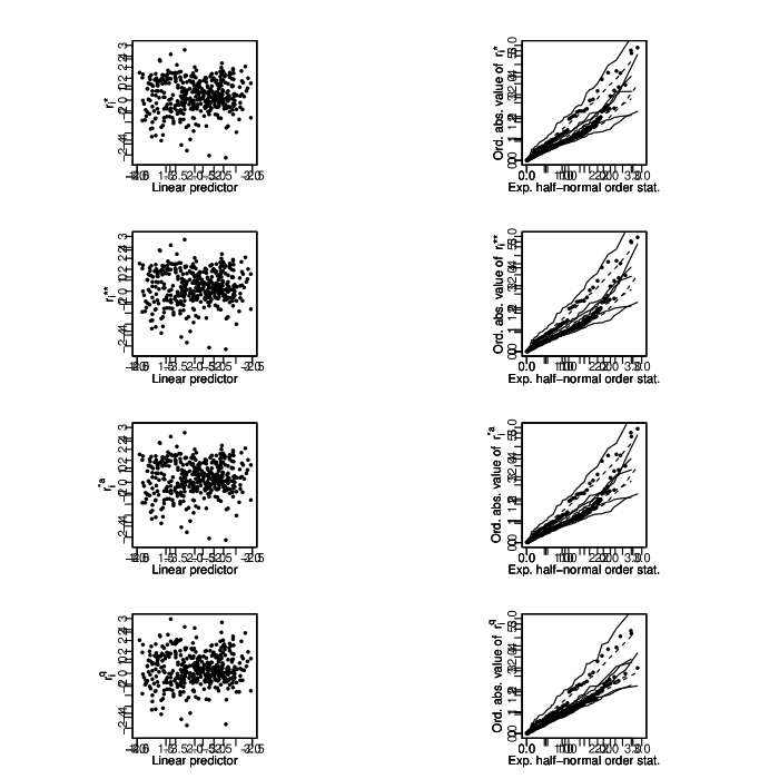
Figure 1: Residuals against linear predictor (left) and half-normal residual plots with simulated envelope (right) for Peruvian election data.

The second application uses data on men professional tennis. The aim is study the proportion of service games won as a function of the number of aces per 5 games of service (AP5GS) and the first service percentage (FSP), that is, the percentage of services that the player got in on his first try. Data were obtained from ATP Website (ATP Tour Inc, 1994) and refer to the performance of the best 50 tennis players of the world in the 10 first months of 2015. Figure 2 presents the residuals plots of the beta regression model with logit link function. None of the residuals suggest model misspecification.

Table 11 presents parameter estimates and standard errors. When the logit link function is used in beta regression, the exponential of the parameters are odds ratios (Ferrari and Cribari-Neto, 2004). It is estimated that for every ace per 5 games increase, FSP held constant, the odds of the proportion of service games won increase by 20.6%. It is also estimated that for every percentage point increase in the first service percentage, AP5GS held constant, the odds of the proportion of service games won increase by 4.2%. The pseudo R² of the fitted regression model is 0.719, suggesting that a substantial proportion of the variability of the proportion of service games won can be explained by a beta regression model with AP5GS and FSP as covariates.

Table 11: Parameter estimates and standard errors for tennis data.

	Estimate	Standard error	Exp(estimate)
Intercept	$-1.421$	$0.470$	$0.241$
AP5GS	$0.187$	$0.026$	$1.206$
FSP	$0.041$	$0.008$	$1.042$

Figure 2: Residuals against linear predictor (left) and half-normal residual plots with simulated envelope (right) for tennis data.

In the second application, none of the residuals suggest model misspecification. However, the simulation studies presented in Section 3 indicated that $r_{i}^{\ast}$, $r_{i}^{\ast\ast}$ and $r_{i}^{\ast^{a}}$ could suggest lack of fit in some scenarios when the beta regression model is correct. To illustrate this fact, we simulated data with 160 observations. Sample size was ten times that used in Section 3 to reduce sample variability. Covariates and response were generated as in Scenario 1 of the simulation studies.

Figure 3 presents the residuals plots of the beta regression model with logit link function. Residuals $r_{i}^{\ast}$, $r_{i}^{\ast\ast}$ and $r_{i}^{\ast^{a}}$ incorrectly suggest model misspecification because there are several residuals lower than $-3$ and four out of the five higher residuals (in absolute value) are outside the boundaries of the simulated envelope. On the other hand, plots of $r_{i}^{q}$ do not suggest lack of fit.

Figure 3: Residuals against linear predictor (left) and half-normal residual plots with simulated envelope (right) for simulated data.

5 Concluding remarks

In this work, we studied the properties of four residuals in beta regression using three applications and Monte Carlo simulation techniques. Five scenarios were simulated for two values of the precision parameter, two sample sizes and two link functions.

It is very desirable that a residual has the following two properties. First, it should be able to detect lack of fit of the model. Second, its distribution should be well approximated by the standard normal distribution. The first application suggested that the four residuals considered in this paper can detect lack of fit of the beta regression model. However, the simulation studies indicated that they are not similar regarding the second property.

In all scenarios, the distribution of the weighted standardized residual 2 is worse approximated by the standard normal distribution than that of the weighted standardized residual 1. In addition, in none of the scenarios, the weighted standardized residual 1 has the closest distribution to the standard normal distribution. Therefore, these residuals do not seem to be the best choice to perform diagnostic analysis in beta regression. The best residual regarding normal approximation depends on the scenario. For $n=40$, except in the case where all mean responses are close to $0.5$, the distribution of the quantile residual is better approximated by the standard normal distribution than that of the adjusted weighted standardized residual 1. This result suggests that the quantile residual is better than the adjusted weighted standardized residual 1 for moderate to large sample sizes. When $n=16$, for most scenarios, the quantile residual is the best for $\phi=10$ and the adjusted weighted standardized residual 1 performs better for $\phi=100$. These findings seem to indicate that, for small sample sizes, the quantile residual is better than the adjusted weighted standardized residual 1 when the variance of the response variable is high, and worse in the low variance case. In addition, the distribution of the quantile residual satisfactorily approximates the standard normal distribution in all scenarios, but the distribution of the adjusted weighted standardized residual 1 displays considerable asymmetry when $\phi$ is small and the mean responses are close to one of the limits of the standard unit interval. This feature of the adjusted weighted standardized residual 1 may lead to incorrect conclusions as shown in the third application.

Besides the advantages shown in the simulation results, the quantile residual has two other advantages compared to the adjusted weighted standardized residual 1: it is simpler and it can be used for any link function. Overall, the quantile residual is therefore a better choice to perform diagnostic analysis in beta regression than the competing residuals.

6 Acknowledgments

The author thanks professor Rafael Izbicki for helpful comments and suggestions on an earlier draft and Fapesp for financial support.

References

• Anholeto et al. (2014) Anholeto, T., Sandoval, M. C., Botter, D. A., 2014. Adjusted pearson residuals in beta regression models. Journal of Statistical Computation and Simulation 84 (5), 999–1014.
• Atkinson (1985) Atkinson, A. C., 1985. Plots, transformations and regression. Clarendon Press, Oxford.
• ATP Tour Inc (1994) ATP Tour Inc, 1994. Atp scores and stats. Accessed: 2015-11-07.
URL http://www.atpworldtour.com/en/stats
• Bayer and Cribari-Neto (2013) Bayer, F. M., Cribari-Neto, F., 2013. Bartlett corrections in beta regression models. Journal of Statistical Planning and Inference 143, 531–547.
• Bayes et al. (2012) Bayes, C. L., Bazán, J. L., García, C., et al., 2012. A new robust regression model for proportions. Bayesian Analysis 7 (4), 841–866.
• Carrasco et al. (2014) Carrasco, J. M. F., Ferrari, S. L. P., Arellano-Valle, R. B., 2014. Errors-in-variables beta regression models. Journal of Applied Statistics 41 (7), 1530–1547.
• Cribari-Neto and Queiroz (2014) Cribari-Neto, F., Queiroz, M. P. F., 2014. On testing inference in beta regressions. Journal of Statistical Computation and Simulation 84 (1), 186–203.
• Cribari-Neto and Zeileis (2010) Cribari-Neto, F., Zeileis, A., 2010. Beta regression in r. Journal of Statistical Software 34 (2), 1–24.
• Doornik (2007) Doornik, J. A., 2007. An Object-Oriented Matrix Language: Ox 5. Timberlake Consultants Press, London.
• Dunn and Smyth (1996) Dunn, P. K., Smyth, G. K., 1996. Randomized quantile residuals. Journal of Computational and Graphical Statistics 5 (3), 236–244.
• Espinheira et al. (2008) Espinheira, P. L., Ferrari, S. L. P., Cribari-Neto, F., 2008. On beta regression residuals. Journal of Applied Statistics 35 (4), 407–419.
• Espinheira et al. (2014) Espinheira, P. L., Ferrari, S. L. P., Cribari-Neto, F., 2014. Bootstrap prediction intervals in beta regressions. Computational Statistics 29, 1263–1277.
• Ferrari and Cribari-Neto (2004) Ferrari, S. L. P., Cribari-Neto, F., 2004. Beta regression for modelling rates and proportions. Journal of Applied Statistics 31 (7), 799–815.
• Figueroa-Zúñiga et al. (2013) Figueroa-Zúñiga, J. I., Arellano-Valle, R. B., Ferrari, S. L. P., 2013. Mixed beta regression: A bayesian perspective. Computational Statistics and Data Analysis 61, 137–147.
• Kieschnick and McCullough (2003) Kieschnick, R., McCullough, B. D., 2003. Regression analysis of variates observed on (0,1): percentages, proportions and fractions. Statistical Modelling 3, 193–213.
• Latif and Zafar Yab (2015) Latif, S., Zafar Yab, M., 2015. D-optimal designs for beta regression models with single predictor. Journal of Statistical Computation and Simulation 85 (9), 1709–1724.
• Lemonte and Bazán (2016) Lemonte, A. J., Bazán, J. L., 2016. New class of johnson sb distributions and its associated regression model for rates and proportions. Biometrical Journal 58 (4), 727–746.
• McCullagh and Nelder (1989) McCullagh, P., Nelder, J. A., 1989. Generalized linear models, 2nd Edition. CRC press, London.
• Nocedal and Wright (2006) Nocedal, J., Wright, S. J., 2006. Numerical Optimization, 2nd Edition. Springer, New York.
• Paolino (2001) Paolino, P., 2001. Maximum likelihood estimation of models with beta-distributed dependent variables. Political Analysis 9 (4), 325–346.
• Rigby and Stasinopoulos (2005) Rigby, R. A., Stasinopoulos, D. M., 2005. Generalized additive models for location, scale and shape. Journal of the Royal Statistics Society: Series C (Applied Statistics) 54 (3), 507–554.
• Stephens (1986) Stephens, M. A., 1986. Tests based on edf statistics. In: D´Agostino, R. B., Stephens, M. A. (Eds.), Goodness-of-fit techniques. Marcel Dekker, New York.