Field of Groves: An Energy-Efficient Random Forest

Abstract

Machine Learning (ML) algorithms, like Convolutional Neural Networks (CNN), Support Vector Machines (SVM), etc. have become widespread and can achieve high statistical performance. However their accuracy decreases significantly in energy-constrained mobile and embedded systems space, where all computations need to be completed under a tight energy budget. In this work, we present a field of groves (FoG) implementation of random forests (RF) that achieves an accuracy comparable to CNNs and SVMs under tight energy budgets. Evaluation of the FoG shows that at comparable accuracy it consumes $\approx$1.48$\times$, $\approx$24$\times$, $\approx$2.5$\times$, and $\approx$34.7$\times$ lower energy per classification compared to conventional RF, SVM_RBF, MLP, and CNN, respectively. FoG is $\approx$6.5$\times$ less energy efficient than SVM_LR, but achieves 18% higher accuracy on average across all considered datasets.

1 Introduction

Over the last couple of decades the consumer market has gradually moved towards mobile computing. According to the comScore report, people of age 18-64 spend $\approx$70% of their digital time using a mobile device [2]. Mobile workloads are increasingly data intensive, and hence machine learning (ML) algorithms are commonly used in these applications [10]. The data-intensive nature of these applications does not allow us to run these applications purely on our mobile systems. For example, applications like speech recognition, although used quite often, are still evaluated remotely because limited energy budgets prohibit running a powerful ML algorithm on a mobile device.

Mobile systems are energy constrained, and hence while designing machine learning architectures for mobile applications we need to manage two conflicting requirements – high accuracy and low energy dissipation. Over the past few years several architecture-, circuit- and algorithm-level optimizations have been proposed for improving the power, performance, area, and accuracy of machine learning accelerator designs [6, 17, 9].

The machine learning community has shown that we do not always require complex classifiers such as convolutional neural networks (CNN) or kernel support vector machines (SVM) for classifying data, and that low-complexity classifiers such as random forests (RFs) are an adequate substitute for applications where high accuracy with low energy dissipation is required [11]. In this paper, we propose an alternative implementation of RF classifiers. We divide the RF into groups of trees called groves for budget-constrained environments, where the budget is accuracy, energy, delay or energy-delay product. In general, RFs are a collection of decision trees (DTs) that independently predict the classification result, with the final decision made by combining the decisions of individual trees. Our approach uses the confidence of groves within the RF about their decision to optimize the resource utilization. In this work:
– We first evaluate the use of RF algorithm as an alternative to CNN, SVM with linear (SVM_LR) and with radial-basis function (SVM_RBF) as the kernels, and Multi-layer Perceptron (MLP) algorithms. Our analysis shows that the RF accuracy is comparable to the accuracy of CNN, SVM_LR, SVM_RBF and MLP for all evaluated datasets, and on average RF consumes $\approx$10$\times$ lower energy per classification.
– We also propose a novel implementation of RF called Field of Groves (FoG). FoG is composed of multiple groves, where every grove is a subset of decision trees. During the evaluation period, the groves start the class probability estimations in parallel, with every grove receiving different inputs. If the probability threshold (confidence level) is not met, the “partially computed” result is issued to the next grove. That way more computational resources are dynamically allocated to examples with higher uncertainty, thus reducing the average cost of estimation. Our evaluation shows that at comparable accuracy FoG consumes $\approx$1.48$\times$, $\approx$24$\times$, $\approx$2.5$\times$, and $\approx$34.7$\times$ lower energy per classification compared to conventional RF, SVM_RBF, MLP, and CNN, respectively, while having similar energy dissipation as SVM_LR.

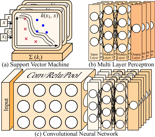
Figure 1: Logical view of SVM, MLP, and CNN.

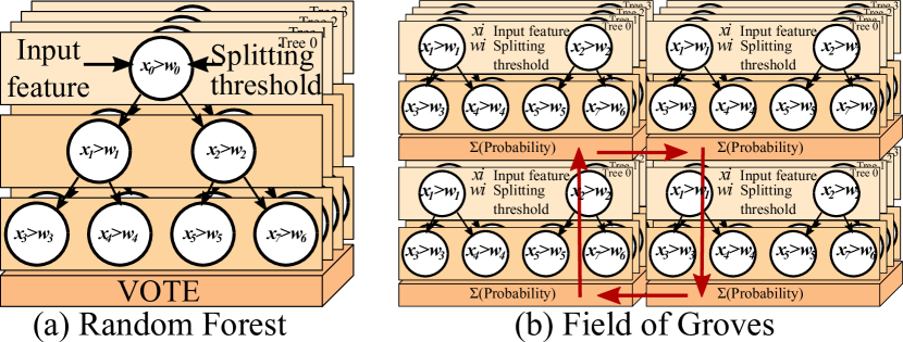
Figure 2: Logical view of RF and FoG.

2 Related Work

Algorithmically, our proposed approach is based on RF classifiers [4]. Traditionally, energy efficiency has not been considered when designing random forests; however, recent work has studied learning of the RFs as a subject to test-time constraints [11]. This approach centers on reducing feature/sensor acquisition cost, however it does not address the system energy constraints. Similar approaches to learning decision rules to minimize error subject to a budget constraint during prediction-time have been proposed [11, 20, 19]. Although closely related, these approaches also ignore the energy usage and disregard computational cost, making them of limited use in an energy constrained settings.

The state of the art machine learning techniques for image processing, video processing, object recognition, etc. are CNN and DNN, and custom hardware accelerator design have been proposed for the same [13]. In addition to that, a variety of techniques including stochastic computing [8], dataflow architecture [5, 12], data reuse [15], custom sparse matrix-vector multiplication [7] and run-time adaptivity [18, 17] have been adopted to achieve energy-efficient machine learning algorithm operation.

The current work proposes a novel implementation of random forest ensemble learning method with the focus on energy-efficient solution to budget constrained evaluation.

3 Random Forests

3.1 Random Forests: Conventional Design

As mentioned in Section 1, we commonly use SVM as well as traditional neural network-based algorithms like CNN or MLP for classifying data sets with large number of features. Figure 1 shows high-level logical view of SVM, MLP, and CNN. In this section we analyze the use of RFs as compared to the popular classification algorithms.

RF is composed of binary decision trees ($DT$) (see Figure 2a), and although the entire RF is composed of $O(t2^{d})$ decisions, where $t$ is the number of trees, and $d$ is the upper bound on the tree depth, evaluation during testing requires only $O(td)$ computations. Every $DT_{i}$ receives some input features $X_{Ri}$, where $X_{Ri}$ is a random subset of input $X$. A “Majority Vote” across trees is then used to identify the label. Such an approach avoids overfitting and ensures high accuracy [4]. Note that during the random forest training, the trees are generated depending on their validation cost, where the cost could be energy, delay, energy-delay product, or accuracy. Turning off DT blocks generally leads to a graceful degradation of accuracy, as the predicted label for a new test example is independent, in contrast to CNN and MLP, where each node in the network is connected to many other nodes, and it is usually difficult to predict how each node affects the accuracy of the the neural network at run-time (it is possible to achieve that offline however). In general, when operating at unlimited energy budgets, CNNs and MLPs generally provide higher accuracy than RF, but RF provides us an opportunity to game accuracy for energy-efficiency. In Section 4, we show more detailed comparison of the classifiers.

Algorithm 1 Constructing Field of Groves Classifier

1:Number of estimators $n>0$; Maximum size of a grove $k\leq n$; Training set $X,y$

2:procedure GCTrain($n,k,X,y$)

3:    Train $RF\leftarrow$ RandomForestTrain($n,X,y$)

4:    return Split(RF, k)

5:end procedure

6: 

7:Subroutine - Splitting a Random Forest

8: 

9:Pretrained random forest $RF$; Maximum size of a grove $k>0$

10:Split grove ensemble $GC$

11:procedure Split($RF,k$)

12:    $i\leftarrow 0$

13:    $GC\leftarrow\emptyset$

14:    while $i<$ Length($RF.estimators$) do

15:         $G\leftarrow$ new Random Forest of size $k$

16:         $G.estimators\leftarrow RF.estimators[i..i+k]$

17:         $GC\leftarrow GC\cup G$

18:         $i\leftarrow i+k$

19:    end while

20:    return GC

21:end procedure

Algorithm 2 Evaluating Field of Groves Classifier

1:Stopping threshold $0<thresh<1$; Maximum number of hops $max\_hops\leq$ Number of groves $n\_groves$; Input set $X$

2:procedure GCEval($X,thresh,max\_hops$)

3:    parallel for every $x$ in $X$

4:         $start\leftarrow$Random(from 0 to $n\_groves$) $\triangleright$ Start at random $grove$ to avoid bias

5:         prob $\leftarrow\{0\}^{\#labels}$

6:         for $j\leftarrow$ from 0 to $max\_hops$ do

7:             $index\leftarrow(start+j)\mod n\_groves$

8:             $\texttt{prob}\leftarrow\texttt{prob}+Grove(index).predict\_prob(x)$

9:             $\texttt{prob\_norm}\leftarrow\texttt{prob}/(j+1)$

10:             if MaxDiff(prob_norm) $\geq thresh$ then

11:                 return prob_norm

12:             end if

13:         end for

14:         return prob_norm

15:    end parallel for

16:end procedure

17: 

18:Subroutine - Minimum Difference of Maximum Values

19: 

20:Array $ar$

21:procedure MaxDiff($ar$)

22:    max1, max2 $\leftarrow$ TwoMaximumValues($ar$)

23:    return abs(max1 - max2) $\triangleright$ In case of “Multi-output classification”, min($\cdot$) function is called prior to returning

24:end procedure

3.2 Random Forests: FoG Implementation

3.2.1 Training and Evaluation Algorithm

As described in section 3.1, RF is suitable for environments where accuracy could be traded-off for energy efficiency. The main advantage of the RF approach stems from the fact that the accuracy of RF tends to improve with an increase in the number of DTs. Moreover, DTs have few active computational nodes during prediction, and the nodes are generally of very low computational complexity. One of the disadvantages that RF experiences is “over-utilization” of the computational resources. Previous works have shown that large portion of input samples within datasets are far enough from the decision boundaries, and do not require complex classifiers [17, 18]. Conventional RFs, however, lack the ability to allocate less computational resources for the inputs if desired. This problem could be solved by using only a limited number of trees, depending on the current confidence level.

In this section we propose a novel RF implementation called Field of Groves (FoG), which avoids any unnecessary expending of energy on inputs with low uncertainty. Each grove is composed of a random, non-overlapping subset of the trees from the “original” RF. Figure 2(b) shows the logical view of our proposed FoG implementation of RF. The training of the FoG is described in Algorithm 1 and is done offline. During this training phase, a RF is first pre-trained (using Algorithm from [11]), and the DTs are randomly split into groves. The splitting involves a simple division of the forest into sets with $k$ DTs, where $k$ is the size of the grove.

The label evaluation algorithm for the approach is shown in Algorithm 2. Here, for every input $x\in X$, we compute the confidence score using one of the randomly selected grove. Confidence in this context is defined as the difference between the most probable and second most probable labels If the confidence is higher than the goal threshold, the computation for $x$ is complete. Otherwise, $x$ and the current probability distribution is sent to the next grove, where the probability array is recomputed again form $x$ and combined with the one received from the previous grove. That way more groves contribute to the inputs with high uncertainty. This process is repeated until either the threshold is exceeded or the the entire forest is evaluated. Note the contrast between FoG and conventional RF evaluation: in FoG the groves return probability distributions which are averaged out across groves; in the conventional RF however the DTs return class predictions, which are later put to a majority vote.

3.2.2 Micro-architecture

The high-level architecture of the FoG implementation of RF is shown on Figure 3. Here, the groves are connected in a circular fashion, with each grove being able to send its current inference to the next grove. To understand the operation of the system, let’s consider an example with a 3-class (class A, class B and class C) problem and the threshold value set to $0.1$. Let us assume that the processor sends an input $X$ that has 5 features. When FoG receives this input, it is assigned an $id$, and is sent to one of the groves (say grove G0 in Figure 3) through the accelerator Input Queue.

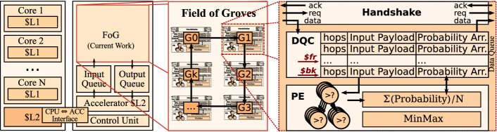
Figure 3: Random Forest implemented as Field of Groves and the microarchitecture of a grove. Notice the grove $G0$ can communicate to grove $G1$ through the “Handshake” block without going out of the FoG. The “Data Queue” includes a controller to maintain pointers $\$fr$ and $\$bk$.

Data Queue
Once $G0$ receives a new input, it places it into the local memory, which serves as a data queue. The queue is controlled using two pointers: $\$fr_{G0}$ and $\$bk_{G0}$ for front and back of the queue respectively. $\$fr_{G0}$ always points to location that contains the input that is currently being processed and $\$bk_{G0}$ points to the first empty location at the back of the queue. For each input we store Input Payload, which holds the received input features + id; Probability Array, which contains the current prediction probabilities; hops which is a count of groves that have so far processed the current Input Payload. Whenever a new input is received: if the input is received from the processor, it is placed at the back of the queue. The Input Payload and Probability array values are set based on the information sent by the processor and the hop count is set to 0. If the input is received from the neighboring grove, it is placed at the front of the queue. The Input Payload and Probability array values are set based on the information sent by the neighboring grove and the hop count is incremented by 1. This ensures that the input that were partially computed have higher priority. In our example, because the input is from the processor, it is placed into the $\$bk_{G0}$ location of the queue. For the new input: {hops = 0, Input Payload = $X$, Probability = {0,0,0}}

Data queue is controlled by the queue controller (DQC) which is responsible for maintaining the $\$fr$ and $\$bk$ pointers. For each received input, DQC routes $\$fr$ to the processing element, the processing element reads the entries corresponding to $\$fr$ and once the computation is complete, it writes the results back to $\$fr$. $\$fr$ and $\$bk$ are incremented by $\Gamma$, which is the length of queue word and represents number of rows in physical memory that are required to store the hop count, Input Payload and Probability Array. $\Gamma$ is a variable, and it depends on the number of features and number of classes in dataset. In our example, $\Gamma=1+5+1+3=10$ (1 byte for hops, 5 bytes for features in Input Payload + 1 byte id, and 3 bytes to store the current label predictionin the Probability Array). Our current implemetation of the FoG has a data queue of 6kB, and can store 8 MNIST examples per grove. Note that the memory can be easily increased to support datasets with larger feature counts and label counts. 

Processing Element (PE)
The PE in every grove is represented by a set of decision trees and its operation is described in algorithm 2. The Input Payload ($X$) is processed by all the trees within the grove to determine the probability distribution of the labels. This result is then averaged with Probability Array received from previous grove or just written back in case of a new input and the current confidence level is computed (as the difference between the two largest values in the Probability Array). The latency of the PE depends on the number of trees per grove, the maximum depth of each tree and degree of parallelism.

Once PE finishes the computation, a decision is made if the current confidence level is adequate. If so, the DQC is notified that the classification of the current Input Payload is complete and the computed result needs to be sent back to the processor. However, if the confidence level is lower than a threshold $thresh$, a request is sent to the next grove for further processing. Here the entire entry (Hop Count, Input Payload and Probability Array) for the current input is copied to the next grove.

Continuing with the previous example, let us say that after $G0$ completes processing the input $X$, it returns the probability distribution of $\{0.32,0.35,0.33\}$. This is used to compute the confidence. In this example the confidence is $0.35-0.33=0.02$. Because the threshold was set at $0.1$, the classification of input $X$ is considered incomplete. It is written back to the location $\$fr_{G0}$, and a req flag in the handshake is raised. At this point, the $fr_{G0}$ is incremented, and grove $G0$ is ready for the next input. The value stored at $\$fr_{G0}-1$ is {hops = 1, Input Payload = $X$, Probability = $\{0.32,0.35,0.33\}$}

Handshaking Protocol
Groves use a simple handshaking protocol to talk with each other. After $G0$ computes the output probabilities, it checks its confidence and if the confidence is low it sets a req flag to signal the neighboring grove $G1$ to copy the current input as well as computed probabilities. Once the copy is complete, an acknowledgment flag ack is raised by $G1$ for one cycle to notify that the copy procedure is complete. At that time $G0$ pulls the req line down, completing the handshake.

Because $G1$ receives its input from another grove (in our case $G0$), it places it at $\$fr_{G1}$ of its queue. Assume that $G1$ computed the probability distribution as $\{0.28,0.45,$ $0.27\}$. These values are averaged with the values computed by $G0$. The entries corresponding to the current input are now {hops = 2, Input Payload = $X$, Probability = $\{0.3,$ $0.4,$ $0.3\}$} and the predicted label is $\operatornamewithlimits{argmax}$ ${(\texttt{Probability})}=1$. At this point, the threshold value constraint is met $0.4-0.3\geq 0.1$, which indicates that this input does not require any further processing, and should be sent to the accelerator output queue. Note that in the example discussed above, the value of hops was increasing with every new grove.

Run-time Tunability
In our proposed FoG implementation of RF the energy-efficiency and accuracy could be easily tuned by changing the probability threshold and maximum hops parameters. The threshold parameter indirectly controls the number of groves that process the input. The maximum hops parameter places an upper limit on the number of groves that process the input (based on EDP or accuracy constraints). A detailed evaluation of how the probability threshold parameter and the maximum hop count parameter affects the energy efficiency and accuracy of our FoG implementation is presented in Section 4.

Reprogrammability
To support various trained RFs corresponding to various datasets, the DTs were implemented to be reprogrammable. For a given dataset, every node is populated with the weights $\omega_{i}$, as well as memory address offsets for the respective features $x_{j}$. In addition to that the DQC is programmable to support variable step for the queue pointer. For example, if a node $N$ checks the conditional $x_{N}>\omega_{N}$, then this node will store the constant $\omega_{N}$, as well as offset $OFF{x_{N}}$. This indicates that the location of the input $x_{N}$ is at $\$fr+OFF{x_{N}}$. At the same time the DQC stores a value $\Gamma$ and the next entry in the queue has an address $\$fr_{next}=\$fr+\Gamma$. The reasoning behind having a variable step size $\Gamma$ is that we want to support different number of features as well as different number of labels for different datasets. For example, MNIST dataset has 784 features and 10 labels, while Penbase Digits dataset has only 16 features and 10 labels.

4 Evaluation

4.1 Experimental Setup

We designed SVM with linear regression kernel (SVM_LR), SVM with Radial-Basis Function kernel (SVM_RBF), MLP, CNN, RF and FoG classifiers for our analysis. To compare the different classifiers we used five different datasets from the UCI library [3], and the list of these datasets is shown in table 1 under the “Dataset” column. These datasets were chosen because they represent a diverse set of workloads typically seen on a mobile device. All the results shown in this section are acquired using the inputs never seen before by the systems under test.

We used the following design flow for performing a detailed power, performance and area comparison of our proposed FoG with other ML classifier algorithms:

Step 1: First, basic computational blocks, such as adders, multipliers, multiply-accumulate (MAC), sigmoid, etc. that are required by all the classifiers are designed considering trade-offs between energy and delay by sweeping through architectural and circuit level parameters, such as bitwidth precision, parallelization, pipelining, etc. We used Aladdin tool [16] to explore the architectural design space, and Cadence tools to extract Power-Performance-Area (PPA) values for each block in this step.

Step 2: Once the library of computational units is generated, it is used in the offline budgeted training described in [11] and algorithm 1. We used energy-delay product (EDP) as budget metric during this phase. If there are several designs that meet the energy constraints, we choose the one with the maximum accuracy. Budgeted training requires information about the costs of building blocks which is provided by the PPA models. We use SciKit-Learn [14] for the training (and exploration of logical structure) of the classifiers.

Step 3: At this step, the detailed hardware microarchitecture of the accelerator is designed. Microarchitecture exploration is independent of training, and is done using Aladdin toolset [16]. The PPA models from the previous step are used during this step to determine Pareto optimal frontier and select the most energy-efficient design.

Step 4: In this final step we design the whole architecture using Chisel HDL [1]. This design environment was chosen, as it generates both hardware description code (Verilog) as well as C++ functional model. That allows for the functionality of the hardware to be verified against software implementation for correctness. The Verilog code was synthesized using 40 $nm$ Global Foundries technology with Synopsys standard cells for detailed power-performance analysis.

FoG Design Considerations
In our implementation, all the classifiers were designed for minimum EDP at maximum accuracy. The FoG classifier was designed from the RF classifier by extracting the pre-trained DTs and re-assembling them into groves. As described above, the number of decision trees per grove and the number of groves is decided during the design time. During the design time we analyzed the EDP and accuracy of different FoG topologies and the minimum EDP design point was selected (while maintaining the accuracy). Figure 4 shows the accuracy and EDP results across different combinations of sizes of groves and total numbers of groves in the FoG.

To illustrate the choice of design time parameters while considering run-time tunability, let us discuss an example with 16 decision trees and ISOLET dataset. After examining the accuracy and EDP of different topologies (see Figure LABEL:fig:dt-sweep:isolet), we isolated two candidate topologies: 8x2 and 4x4. At this point we can use the “run-time tunability” as a deciding factor between these two roughly equivalent candidate topologies. Figure 5 shows the accuracy and EDP across all datasets as a function of threshold. Figure LABEL:fig:tuning:8-2 shows that 8x2 topology is more energy-efficient, but the accuracy is lower for lower threshold settings. Figure LABEL:fig:tuning:4-4 shows, in contrast, that the accuracy penalty for lower thresholds is not as drastic, but the energy-efficiency penalty is higher. In our case we go with 8x2 topology as minimum EDP is our primary goal. Note that once the physical topology is selected, the “threshold” variable could be changed during run-time to achieve a different operating point.

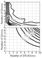
(a)

(b)

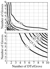
(c)

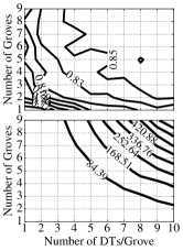
(d)

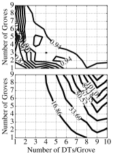
(e)

Figure 4: Accuracy and EDP as a function of “Number of Groves” and the “Number of Decision Trees per Grove”. The product of the two variables shows the total number of decision trees in the FoG.

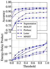
(a)

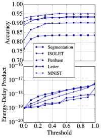
(b)

Figure 5: Example of FoG run-time tuning using the “threshold” variable.

4.2 Experimental Results

To perform a comparison of the classifier algorithms listed in section 4.1, we first trained all the algorithms for their maximum accuracy without worrying about energy efficiency. Table 1 shows the comparison of accuracy between different classifiers. Two different numbers for the FoG are reported: FoG_max and FoG_opt. FoG_max shows the results for the FoG with its “threshold” parameter set to maximum. This forces the FoG to behave like an RF because every input will have to go through every decision tree of every grove. FoG_opt shows the results for the case when confidence threshold was set to accuracy optimal point – a threshold point above which accuracy does not increase with threshold but below which accuracy decreases with decrease in threshold.

From the table we can see that CNN has the highest accuracy for all datasets. The accuracy of the traditional RF classifier is comparable to CNN for all datasets. In terms of energy per classification, RF consumes $\approx$15$\times$, $\approx$1.7$\times$, and $\approx$23.5$\times$ less energy than SVM_RBF, MLP and CNN, respectively. The RF energy consumption is $\approx$10$\times$ higher than that of SVM_LR, but RF on average provides 20% higher accuracy than linear SVM. The very low energy dissipation in RF is due to the fact that the basic computational unit in a DT is very simple (a basic comparator).

Table 1 also shows the accuracy and energy dissipation of our proposed FoG implementation of the RF classifier. Here all classifiers have been designed to operate at 1 $GHz$. The maximum achievable accuracy of the FoG (both $max$ and $opt$) implementation is lower than RF and CNN by 3.2% and 4%, respectively, but FoG_opt classifier consumes $\approx$1.5$\times$ and $\approx$34.7$\times$ lower energy than RF and CNN, respectively. The FoG_max on average consumes almost the same amount of energy energy as RF, and $\approx$23$\times$ lower than CNN. When comparing to the SVMs, the accuracy of the FoG classifier outperforms the linear support vector machine SVM_LR by $\approx$15% on average, and achieves comparable statistical performance when compared to the SVM_RBF. In terms of energy SVM_LR is $\approx$10$\times$ more efficient on average, while SVM_RBF is more expensive ($\approx$23.6$\times$ higher energy consumption when compared to FoG_opt).

The main advantage of the FoG is that while achieving statistical performance comparable to the performance of the RF, it also allows easy run-time change in the energy-accuracy trade-off. Figure 5 shows how accuracy could be traded off for energy for 8x2 and 4x4 FoG topologies. Figure LABEL:fig:tuning:8-2 shows that energy-efficiency could be easily improved by an order of magnitude without sacrificing much accuracy by tuning the confidence threshold from $1.0$ to $0.5$ for most datasets. After that a “trade-off” region of tunability starts – one can improve energy-efficiency by trading off accuracy. This run-time tuning opportunity will prove beneficial in environments with constraint energy. The figure shows that for 8x2 design, two orders of magnitude improvement in energy efficiency could be achieved by tuning the confidence threshold from $0.5$ to $<0.1$. The accuracy drop in case of aggressive confidence tuning is anywhere between 10% to 30% depending on the dataset. The story is similar for 4x4 topology (figure LABEL:fig:tuning:8-2), however, the “trade-off” region of tunability starts at confidence threshold of $\approx$0.3. Although the accuracy drop is not as drastic, the EDP for 4x4 topology is much higher – an order of magnitude higher for low accuracy, and equivalent for high accuracy points.

Table 1 also shows the area comparison between different classifiers. It must be noted that most classifiers’ area changes drastically with the internal parameters – e.g. convolutional layers sometimes implemented as having “volume” activation, and changing the size of one layer, might contribute to the total area change cubically. Overall, the area of our FoG implementation is larger than all classifiers except CNN.

	SVM					FoG
Dataset	${lr}$	${rbf}$	MLP	CNN	RF	$max$	$opt$
ISOLET	69	93	87	94	92	91	90
Penbase	86	95	91	96	96	93	93
MNIST	82	95	87	96	96	94	93
Letter	78	93	93	96	95	85	85
Segment.	67	91	91	96	95	94	92
ISOLET	5.9	980	82.5	1150	41	49	30
Penbase	0.4	18	13.3	186	16	14	7.1
MNIST	6.1	1020	93	1300	43	47	38
Letter	0.5	19	13.7	192	16	12.9	7.6
Segment.	0.6	26	14.5	203	13	9	4.7
Area	0.13	0.53	0.93	2.1	1.38	1.9	1.9

Table 1: Accuracy (top) and Energy dissipation (bottom) in nJ per classification for different datasets [3]. Frequency is fixed at 1 $GHz$ for all datasets. SVM_lr and SVM_rbf show the results for SVM with linear and RBF kernels; FoG_max and FoG_opt show the results for FoG with its threshold set to maximum and to the optimal accuracy tuning point, respectively. The area results are in mm²

.

5 Conclusion

In this work we have compared the lightweight RF classification algorithm with heavyweight classification algorithms like CNN, MLP, and SVM in terms of accuracy and energy efficiency. We proposed a novel FoGs approach to RF implementation that can dynamically trade-off accuracy for energy efficiency at run time, while achieving accuracy comparable to traditional RFs. The proposed FoG approach examines decision confidence for each input, and allocates the computational resources depending on the input’s uncertainty levels. We implemented the FoG using a 40 nm technology, and tested it using the datasets provided by the UCI repository. The evaluation results show that the accuracy of the traditional RF classifier is comparable (if not larger) to CNN for all datasets that we considered and at the same time RF consumes $\approx$15$\times$, $\approx$1.7$\times$, and $\approx$23$\times$ less energy than SVM_RBF, MLP and CNN, respectively. The maximum achievable accuracy of the FoG implementation is lower than RF and CNN by 3.2% and 4%, respectively, but FoG classifiers have $\approx$1.7$\times$ and $\approx$35$\times$ lower energy than RF and CNN, respectively.

References

- [1] Chisel: Constructing hardware in an scala embedded language. https://chisel.eecs.berkeley.edu/.
- [2] comScore: The 2016 U.S. Mobile App Report. http://www.comscore.com/Insights/Presentations-and-Whitepapers/2016/The-2016-US-Mobile-App-Report.
- [3] UCI Machine Learning. http://archive.ics.uci.edu/ml/.
- [4] L. Breiman. Random forests. Machine Learning, 2001.
- [5] Y. H. Chen, J. Emer, and V. Sze. Eyeriss: A spatial architecture for energy-efficient dataflow for convolutional neural networks. In ISCA, 2016.
- [6] Z. Du, D. D. B. D. Rubin, Y. Chen, L. Hel, T. Chen, L. Zhang, C. Wu, and O. Temam. Neuromorphic accelerators: A comparison between neuroscience and machine-learning approaches. In Proc., MICRO-48, 2015.
- [7] S. Han, X. Liu, H. Mao, J. Pu, A. Pedram, M. A. Horowitz, and W. J. Dally. Eie: efficient inference engine on compressed deep neural network. arXiv:1602.01528, 2016.
- [8] K. Kim, J. Kim, J. Yu, J. Seo, J. Lee, and K. Choi. Dynamic energy-accuracy trade-off using stochastic computing in deep neural networks. In DAC’15.
- [9] M. Kusner, W. Chen, Q. Zhou, Z. E. Xu, K. Weinberger, and Y. Chen. Feature-cost sensitive learning with submodular trees of classifiers. In AAAI’14.
- [10] N. D. Lane, E. Miluzzo, H. Lu, D. Peebles, T. Choudhury, and A. T. Campbell. A survey of mobile phone sensing. Communications Magazine, IEEE, 2010.
- [11] F. Nan, J. Wang, and V. Saligrama. Feature-budgeted random forest. In ICML’15.
- [12] T. Nowatzki, V. Gangadhar, and K. Sankaralingam. Exploring the potential of heterogeneous von neumann/dataflow execution models. In ISCA, 2015.
- [13] S. Park, K. Bong, D. Shin, J. Lee, S. Choi, and H. J. Yoo. 4.6 a1. 93tops/w scalable deep learning/inference processor with tetra-parallel mimd architecture for big-data applications. In ISSCC, 2015.
- [14] F. Pedregosa, G. Varoquaux, A. Gramfort, V. Michel, B. Thirion, O. Grisel, M. Blondel, P. Prettenhofer, R. Weiss, V. Dubourg, J. Vanderplas, A. Passos, D. Cournapeau, M. Brucher, M. Perrot, and E. Duchesnay. Scikit-learn: Machine learning in Python. JMLR, 12, 2011.
- [15] A. Rahman, J. Lee, and K. Choi. Efficient fpga acceleration of convolutional neural networks using logical-3d compute array. In DATE, 2016.
- [16] Y. S. Shao, B. Reagen, G.-Y. Wei, and D. Brooks. Aladdin: A pre-rtl, power-performance accelerator simulator enabling large design space exploration of customized architectures. In ISCA, 2014.
- [17] Z. Takhirov, J. Wang, V. Saligrama, and A. Joshi. Energy-efficient adaptive classifier design for mobile systems. In ISLPED 2016.
- [18] S. Venkataramani, A. Raghunathan, J. Liu, and M. Shoaib. Scalable-effort classifiers for energy-efficient machine learning. In DAC, 2015.
- [19] J. Wang, K. Trapeznikov, and V. Saligrama. Efficient learning by directed acyclic graph for resource constrained prediction. In NIPS. 2015.
- [20] Z. E. Xu, K. Q. Weinberger, and O. Chapelle. The greedy miser: Learning under test-time budgets. In ICML, 2012.