Abstract.

In various economic environments, people observe other people with whom they strategically interact. We can model such information-sharing relations as an information network, and the strategic interactions as a game on the network. When any two agents in the network are connected either directly or indirectly in a large network, empirical modeling using an equilibrium approach can be cumbersome, since the testable implications from an equilibrium generally involve all the players of the game, whereas a researcher’s data set may contain only a fraction of these players in practice. This paper develops a tractable empirical model of linear interactions where each agent, after observing part of his neighbors’ types, not knowing the full information network, uses best responses that are linear in his and other players’ types that he observes, based on simple beliefs about the other players’ strategies. We provide conditions on information networks and beliefs such that the best responses take an explicit form with multiple intuitive features. Furthermore, the best responses reveal how local payoff interdependence among agents is translated into local stochastic dependence of their actions, allowing the econometrician to perform asymptotic inference without having to observe all the players in the game or having to know the precise sampling process.

Key words. Strategic Interactions; Behavioral Modeling; Information Sharing; Games on Networks; Cross-Sectional Dependence

JEL Classification: C12, C21, C31

1. Introduction

Interactions between agents - for example, through personal or business relations - generally lead to their actions being correlated. In fact, such correlated behaviors form the basis for identifying and estimating peer effects, neighborhood effects, or more generally, social interactions in the literature. (See Blume/Brock/Durlauf/Ioannides:11:HandbookSE and Durlauf/Ioannides:10:ARE for a review of this literature.)

Empirical modeling becomes nontrivial when one takes seriously the fact that people are often connected directly or indirectly on a large complex network, and observe some of their neighbors’ types. Such strategic environments may be highly heterogeneous across agents, with each agent occupying a nearly “unique” position in the network. Information sharing potentially creates a complex form of cross-sectional dependence among the observed actions of agents, yet the econometrician typically observes only a fraction of the agents on the network, and rarely observes the entire network which governs the cross-sectional dependence structure.

The main contribution of this paper is to develop a tractable empirical model of linear interactions among agents with the following three major features. First, assuming a large game on a complex, exogenous network, our empirical model does not require the agents to observe the full network. Instead, we assume that each agent observes only a local network around herself and only part of the type information of those who are local to her.

Second, our model explains strategic interdependence among agents through correlated observed behaviors. In this model, the cross-sectional local dependence structure among the observed actions reflects the network of strategic interdependence among the agents. Most importantly, unlike most incomplete information game models in the literature, our set-up allows for information sharing on unobservables, i.e., each agent is allowed to observe his neighbors’ payoff-relevant signals that are not observed by the econometrician.

Third, the econometrician does not need to observe the whole set of players in the game for inference. It suffices that he observe many (potentially) non-random samples of local interactions. The inference procedure that this paper proposes is asymptotically valid independently of the actual sampling process, as long as the sampling process satisfies certain weak conditions. Accommodating a wide range of sampling processes is useful because random sampling is rarely used for the collection of network data, and a precise formulation of the actual sampling process is often difficult in practice.

A standard approach for studying social interactions is to model them as a game, and use the game’s equilibrium strategies to derive predictions and testable implications. Such an approach is cumbersome in our set-up. Since a particular realization of any agent’s type affects all the other agents’ equilibrium actions through a chain of information sharing, each agent needs to form a “correct” belief about the entire information graph. Apart from such an assumption being highly unrealistic, it also implies that predictions from an equilibrium that generate testable implications usually involve all the players in the game, when it is often the case that only a fraction of the players are observed in practice. Thus, an empirical analysis which regards the players in the researcher’s sample as coincident with the actual set of players in the game may suffer from a lack of external validity when the target population is a large game involving many more players than those present in the actual sample.

Instead, this paper adopts an approach of behavioral modeling, where it is assumed that each agent, not knowing fully the information sharing relations, optimizes according to simple beliefs about the other players’ strategies. The crucial part of our behavioral assumption is a primitive form of belief projection which says that each agent, not knowing the full set of information-sharing relations, projects his own beliefs about other players onto his payoff neighbors. More specifically, if agent $i$ gives more weight to agent $j$ than to agent $k$, agent $i$ believes that each of his payoff neighbors $s$ does the same in comparing agents $j$ and $k$. Here the “weights” represent the strategic importance of other players, and belief projection can be viewed as a rule-of-thumb for an agent who needs to form expectations of the actions of the players, not knowing who they observe. When the strategic importance of one player to another is based primarily on “vertical” characteristics such as skills or assets, the assumption of belief projection does not seem unrealistic.

Our belief projection approach yields an explicit form of the best response which has intuitive features. For example, the best response is such that each agent $i$ gives more weight to those agents with a higher local centrality to him, where the local centrality of agent $j$ to agent $i$ is said to be high if and only if a high fraction of agents whose actions affect agent $i$’s payoff have their payoffs affected by agent $j$’s action. Also, the best response is such that each agent responds to a change in his own type more sensitively when there are stronger strategic interactions, due to what we call the reflection effect. The reflection effect of player $i$ captures the way that player $i$’s type affects his own action through his payoff neighbors whose payoffs are affected by player $i$’s types and actions.

The best responses reveal an explicit form of local dependence among the observed actions from which we can derive minimal conditions for feasible asymptotic inference. It turns out that the econometrician does not need to observe all the players in the game, nor does he need to know the precise sampling process. Furthermore, the best response from the belief assumption provides a testable implication for information sharing on unobservables in data. In fact, the cross-sectional correlation of residuals indicates information sharing on unobservables. (See the Supplemental Note for details on the testing procedure based on the cross-sectional correlation of residuals.)

It is instructive to compare the predictions from our behavioral model to those from an equilibrium model. When the payoff graph is comprised of multiple disjoint subgraphs that are complete, the behavioral strategies and equilibrium strategies coincide. Moreover, for a game on a general payoff graph, we show that as the rationality of agents deepens and their information expands, the behavioral strategies converge to the equilibrium strategies of an incomplete information game where each agent observes all the sharable types of every other agent.

We provide conditions under which the parameters are locally identified, but propose asymptotic inference in a general setting that does not require such conditions. We also investigate the finite sample properties of our asymptotic inference through Monte Carlo simulations using various payoff graphs. The results show reasonable performance of the inference procedures. In particular, the size and the power of the test for the strategic interaction parameter are good in finite samples. We apply our methods to an empirical application which studies the decision of state presence by municipalities, revisiting Acemoglu/GarciaJimeno/Robinson:15:AER. We consider an incomplete information game model which permits information sharing on unobservables. The fact that our best responses explicitly reveal the local dependence structure means that it is unnecessary to separately correct for spatial correlation following, for example, the procedure of Conley:99:JOE.

The literature on social interactions often looks for evidence of interactions through correlated behaviors. For example, linear interactions models investigate correlation between the outcome of an agent $i$ and the average outcome over agent $i$’s neighbors. See for example Manski:93:Restud, DeGiorgi/Pellizzari/Redaelli:10:AEJ, Bramoulle/Djebbari/Fortin:09:JOE and Blume/Brock/Durlauf/Jayaraman:15:JPE for identification analysis in linear interactions models, and see Calvo-Armengol/Pattacchini/Zenou:09:ReStud for an application to the study of peer effects. Goldsmith-Pinkham/Imbens:13:JBES considers nonlinear interactions on a social network and discusses endogenous network formation. Such models often assume that the researcher observes many independent samples of such interactions, where each independent sample constitutes a game containing the entire set of the players in the game.

In the context of a complete information game, a linear interaction model on a large social network can generally be estimated without assuming independent samples. The outcome equations in such a setting frequently take the form of spatial autoregressive models, which have been actively studied in the spatial econometrics literature (Anselin:88:SpatialEconometrics). A recent study by Johnsson/Moon:16:WP considers a model of linear interactions on a large social network which allows for endogenous network formation. Developing inference on a large game model with nonlinear interactions is more challenging. See Menzel:16:ReStud, Xu:15:WP, Song:14:WP, Xu/Lee:15:WP, and Yang/Lee:16:JOE for a large game model of nonlinear interactions. This large game approach is suitable when the data set does not have many independent samples of interactions. One of the major issues in the large game approach is that the econometrician often observes only a subset of the agents from the original game of interest.

Our empirical approach is based on a large game model which is close to models of linear interactions in the sense that it attempts to explain strategic interactions through the correlated behavior of neighbors. In our set-up, the cross-sectional dependence of the observed actions is not merely a nuisance that complicates asymptotic inference; it provides the very information that reveals the nature of strategic interdependence among agents. Such correlated behavior also arises in equilibrium in models of complete information games or games with types that are either privately or commonly observable. (See Bramoulle/Djebbari/Fortin:09:JOE and Blume/Brock/Durlauf/Jayaraman:15:JPE.) However, as emphasized before, such an approach can be cumbersome in our context of a large game primarily because the testable implications from the model typically involve the entire set of players, when in many applications the econometrician observes only a small subset of the game’s players. After finishing the first draft of paper, we learned of a recent paper by Eraslan/Tang:17:WP who model the interactions as a Bayesian game on a large network with private link information. They do not require the agents to observe the full network, and show identification of the model primitives adopting a Bayesian Nash equilibrium as a solution concept. One of the major differences of our paper from theirs is that our paper permits information sharing on unobservables, so that the actions of neighboring agents are potentially correlated even after controlling for observables.

A departure from the equilibrium approach in econometrics is not new in the literature. Aradillas-Lopez/Tamer:08:JBES studied implications of various rationality assumptions for identification of the parameters in a game. Unlike their approach, our focus is on a large game where many agents interact with each other on a single complex network, and, instead of considering all the beliefs which rationalize observed choices, we consider a particular set of beliefs that satisfy a simple rule and yield an explicit form of best responses. (See also Goldfarb/Xiao:11:AER and Hwang:17:WP for empirical research adopting behavioral modeling for interacting agents.)

This paper is organized as follows. In Section 2, we introduce an incomplete information game of interactions with information sharing. This section derives the crucial result of best responses under simple belief rules. We also show the convergence of behavioral strategies to equilibrium strategies as the rationality of agents becomes higher and their information sets expand. Section 3 focuses on econometric inference. It explains the data set-up and a method for constructing confidence intervals. Section 4 investigates the finite sample properties of our inference procedure through a Monte Carlo study. Section 5 presents an empirical application on state capacity among municipalities. Section 6 concludes. Due to the space constraints, the technical proofs of the results are found in the Supplemental Note of this paper. The Supplemental Note also contains other materials including extensions to a model of information sharing among many agents over time, testing for information sharing on unobservables, and a model selection procedure for choosing among different behavioral models.

2. Strategic Interactions with Information Sharing

2.1. A Model of Interactions with Information Sharing

Strategic interactions among a large number of information-sharing agents can be modeled as an incomplete information game. Let $N$ be the set of a finite yet large number of players. Each player $i\in N$ is endowed with his type vector $(\tau_{i},\eta_{i})$, where $\eta_{i}$ is a private type and $\tau_{i}$ a sharable type. As we will elaborate later, information $\eta_{i}$ is kept private to player $i$ whereas $\tau_{i}$ is observed by his neighbors in a network which we define below.

To capture strategic interactions among players, let us introduce an undirected graph $G_{P}=(N,E_{P})$, where $E_{P}$ denotes the set of edges $ij$, $i,j\in N$ with $i\neq j$, and each edge $ij\in E_{P}$ represents that the action of player $i$ affects player $j$’s payoff. We denote $N_{P}(j)$ to be the $G_{P}$-neighborhood of player $j$, i.e., the collection of players whose actions affect the payoff of player $j$:

$$N_{P}(j)=\{i\in N:ij\in E_{P}\},$$

and let $n_{P}(j)=|N_{P}(j)|.$ We define $\overline{N}_{P}(j)=N_{P}(j)\cup\{j\}$ and let $\overline{n}_{P}(j)=|\overline{N}_{P}(j)|$.

Player $i$ choosing action $y_{i}\in\mathcal{Y}$ with the other players choosing $y_{-i}=(y_{j})_{j\neq i}$ obtains payoff:

(2.1) $$u_{i}(y_{i},y_{-i},\tau,\eta_{i}) = y_{i}\left(\tau_{i}+\beta_{0}\overline{y}_{i}+\eta_{i}\right)-\frac{1}{2}y_{i}^{2},$$

where $\tau=(\tau_{i})_{i\in N}$, and

$$\overline{y}_{i}=\frac{1}{n_{P}(i)}\sum_{k\in N_{P}(i)}y_{k},$$

if $N_{P}(i)\neq\varnothing$, and $\overline{y}_{i}=0$ otherwise. Thus the payoff depends on other players’ actions and types only through those of his $G_{P}$-neighbors. We call $G_{P}$ the payoff graph.

The parameter $\beta_{0}$ measures the payoff externality among agents. As for $\beta_{0}$, we make the following assumption:

Assumption 2.1.

$-1<\beta_{0}<1.$

This assumption is commonly used to characterize a pure strategy equilibrium in the social interactions literature. (See e.g. Bramoulle/Djebbari/Fortin:09:JOE and Blume/Brock/Durlauf/Jayaraman:15:JPE for examples of its use.) When $\beta_{0}>0$, the game is called a game of strategic complements and, when $\beta_{0}<0$, a game of strategic substitutes.

Let us introduce information sharing relations in the form of a directed graph (or a network) $G_{I}=(N,E_{I})$ on $N$ so that each $ij$ in $E_{I}$ represents the edge from player $i$ to player $j$, where the presence of edge $ij$ joining players $i$ and $j$ indicates that $\tau_{i}$ is observed by player $j$. Hence the presence of an edge $ij$ between agents $i$ and $j$ represents information flow from $i$ to $j$. This paper calls graph $G_{I}$ the information graph. For each $j\in N$, define

$$N_{I}(j)=\{i\in N:ij\in E_{I}\},$$

that is, the set of $G_{I}$-neighbors observed by player $j$. Also let $\overline{N}_{I}(i)=N_{I}(i)\cup\{i\}$, and $\overline{n}_{I}(i)=|\overline{N}_{I}(i)|$.

In this paper, we do not assume that each agent knows the whole information graph $G_{I}$ and the payoff graph $G_{P}$. To be precise about each agent’s information set, let us introduce some notation. For each $i\in N$, we set $\overline{N}_{P,1}(i)=\overline{N}_{P}(i)$ and $\overline{N}_{I,1}(i)=\overline{N}_{I}(i)$, and for $m\geq 2$, define recursively

$$\overline{N}_{P,m}(i)=\bigcup_{j\in\overline{N}_{P}(i)}\overline{N}_{P,m-1}(j),\textnormal{ and }\overline{N}_{I,m}(i)=\bigcup_{j\in\overline{N}_{I}(i)}\overline{N}_{I,m-1}(j).$$

Thus $\overline{N}_{P,m}(i)$ denotes the set of players which consist of player $i$ and those players who are connected to player $i$ through at most $m$ edges in $G_{P}$, and similarly with $\overline{N}_{I,m}(i)$. Also, define $N_{P,m}(i)=\overline{N}_{P,m}(i)\setminus\{i\}$ and $N_{I,m}(i)=\overline{N}_{I,m}(i)\setminus\{i\}$.

For each player $i\in N$, let us introduce a local payoff graph $G_{P,m}(i)=(\overline{N}_{P,m}(i),E_{P,m}(i))$, where for $k_{1},k_{2}\in\overline{N}_{P,m}(i)$, $k_{1}k_{2}\in E_{P,m}(i)$ if and only if $k_{1}k_{2}\in E_{P}$. Define for $m\geq 1$,

(2.2) $$\mathcal{I}_{i,m-1}=(G_{P,m+1}(i),\overline{N}_{I,m}(i),\tau_{\overline{N}_{I,m}(i)},\eta_{i}),$$

where $\tau_{\overline{N}_{I,m}(i)}=(\tau_{j})_{j\in\overline{N}_{I,m}(i)}$. We use $\mathcal{I}_{i,m}$ to represent the information set of agent $i$. For example, when agent $i$ has $\mathcal{I}_{i,0}$ as his information set, it means that agent $i$ knows the payoff subgraph $G_{P,2}$ among the agents $\overline{N}_{P,2}(i)$, the set of agents whose types he observes (i.e., $N_{I}(i)$), and his own private signal $\eta_{i}$. As for the payoff graph and information graph, we make the following assumption.

Assumption 2.2.

For each $i\in N$ and $m\geq 1$,

$$\overline{N}_{P,m+1}(i)\subset\overline{N}_{I,m}(i).$$

This assumption requires for example that an agent with information $\mathcal{I}_{i,0}$ observes their $G_{P}$ neighbors and their payoff relevant neighbors. The assumption on $G_{I}$ only requires what each set $\overline{N}_{I,m}(i)$ should at least include but not what it should exclude. Hence all the results of this paper carry through even if we have $\overline{N}_{I,m}(i)=N$ for all $i\in N$, as in a complete information game. In other words, the incomplete information feature of our game is permitted but not required for our framework.

2.2. Predictions from Rationality

Each player chooses a strategy that maximizes his expected payoff according to his beliefs. Given player $i$’s strategy, information set $\mathcal{I}_{i}$, and his beliefs on the strategy of other players $s_{-i}^{i}=(s_{k}^{i})_{k\in N\setminus\{i\}}$, the (interim) expected payoff of player $i$ is defined as

$$U_{i}(s_{i},s_{-i}^{i};\mathcal{I}_{i})=\mathbf{E}[u_{i}(s_{i}(\mathcal{I}_{i}),s_{-i}^{i}(\mathcal{I}_{-i}),\tau,\eta_{i})|\mathcal{I}_{i}],$$

where $s_{-i}^{i}(\mathcal{I}_{-i})=(s_{k}^{i}(\mathcal{I}_{k}))_{k\in N\setminus\{i\}}$, $\mathcal{I}_{-i}=(\mathcal{I}_{k})_{k\neq i}$ and $\tau=(\tau_{i})_{i\in N}$. A best response $s_{i}^{\textsf{BR}}$ of player $i$ corresponding to the strategies $s_{-i}^{i}$ of the other players as expected by player $i$ is such that for any strategy $s_{i}$,

$$U_{i}(s_{i}^{\textsf{BR}},s_{-i}^{i};\mathcal{I}_{i})\geq U_{i}(s_{i},s_{-i}^{i};\mathcal{I}_{i}),\textnormal{ a.e.}$$

The quadratic payoff function and the information structure of the game implies that if player $i$ has information set $\mathcal{I}_{i}$ and believes that each of her $G_{P}$-neighbors, say, $k$, plays a strategy $s_{k}^{i}(\mathcal{I}_{k})$, her best response is given by

(2.3) $$s_{i}^{\textsf{BR}}(\mathcal{I}_{i})=\tau_{i}+\frac{\beta_{0}}{n_{P}(i)}\sum_{k\in N_{P}(i)}\mathbf{E}[s_{k}^{i}(\mathcal{I}_{k})|\mathcal{I}_{i}]+\eta_{i}.$$

This implies that the best responses will be linear in types $\tau_{j}$ as long as the conditional expectation is.

In order to generate predictions, one needs to deal with the beliefs (i.e., $s_{k}^{i}(\mathcal{I}_{k})$) in the conditional expectation. There are three approaches. The first approach is an equilibrium approach, where we take the predicted strategies as a set of best response strategies $s_{i}^{\textsf{BNE}}$ such that for any strategy $s_{i}$,

(2.4) $$U_{i}(s_{i}^{\textsf{BNE}},s_{-i}^{\textsf{BNE}};\mathcal{I}_{i})\geq U_{i}(s_{i},s_{-i}^{\textsf{BNE}};\mathcal{I}_{i}),\textnormal{ a.e.}$$

Hence in equilibrium strategies, each player believes that the other players’ strategies coincide with the best response strategies by the agents in equilibrium. The second approach, rationalizability, considers all strategies that are rationalizable given some belief. The third approach is a behavioral approach where one considers a set of simple behavioral assumptions on the beliefs and focuses on the best responses to these beliefs.

There are pros and cons with each of the three approaches. The equilibrium approach requires that the beliefs of all the players be “correct” in equilibrium. However, since each player $i$ generally does not know who each of his $G_{P}$-neighbors observes, a Bayesian player in an incomplete information game with rational expectations would need to know the distribution of the entire information graph $G_{I}$ (or at least have a common prior on the information graph commonly agreed upon by all the players) to form a “correct” belief given his information. Given that the players are only partially observed and $G_{I}$ is rarely observed with precision, producing a testable implication from such an equilibrium model appears far from a trivial task.

The rationalizability approach can be used to relax this rational expectations assumption by eliminating the requirement that the beliefs be correct. Such an approach considers all the predictions that are rationalizable given some beliefs. However, the set of predictions from rationalizability can potentially be large and may fail to produce sharp predictions useful in practice.

This paper takes the approach of behavioral modeling. We adopt a set of simple behavioral assumptions on players’ beliefs which can be incorrect from the viewpoint of a person with full knowledge of the distribution of the information graph, yet useful as a rule-of-thumb for an agent in a complex decision-making environment such as the one in our model. As we shall see later, this approach can give a sharp prediction that is intuitive and analytically tractable. Furthermore, the best responses from this approach coincide with equilibrium strategies for a special class of payoff graphs, and converge to equilibrium strategies for any payoff graph as the rationality of agents becomes deeper and their information set expands.

2.3. Belief Projection and Best Responses

2.3.1. A Game with Complete Payoff Subgraphs

Let us consider first a special case where the payoff graph $G_{P}=(N,E_{P})$ is such that $N$ is partitioned into subsets $N_{1},...,N_{Q}$, and for all $i,j\in N$ with $i\neq j$, $ij\in E_{P}$ if and only if $i,j\in N_{q}$ for some $q=1,...,Q$. In this game, there are multiple strategically disjoint subgames and agents in each subgame observe all other players’ sharable types $\tau_{j}$’s in the subgame, but do not observe their private types $\eta_{j}$. In this case, there exists a unique Bayesian Nash equilibrium where the equilibrium strategies take the explicit form of a linear strategy: for each player $i$,

$$s_{i}(\mathcal{I}_{i,0})=\sum_{j\in\overline{N}_{P}(i)}\tau_{j}w_{ij}+\eta_{i},$$

and $w_{ij}$ are weights such that for all $i,j,k,\ell$ in the same cluster,

(2.5) $$w_{kk}=w_{ii},\text{ and }w_{k\ell}=w_{ij},\text{ whenever }i\neq j\text{ and }k\neq\ell.$$

Thus the equilibrium is within-cluster symmetric in the sense that the equilibrium strategy is the same across all the agents in the same cluster. However, this symmetric equilibrium does not extend to a general payoff graph $G_{P}$.

2.3.2. Belief Projection

Our approach uses a weaker version of the symmetry restrictions (2.5) to specify initial beliefs, so that a best response function exists uniquely for any payoff graph configuration. More specifically, we introduce the following symmetry restrictions on the belief formation.

Definition 2.1.

We say that a player $i$ with information set $\mathcal{I}_{i,0}$ does BP (Belief Projection), if she believes that each of her $G_{P}$-neighbors, say, $k$, plays a linear strategy as:

(2.6) $$s_{k}^{i}(\mathcal{I}_{k,0})=\sum_{j\in\overline{N}_{P}(k)}\tau_{j}w_{kj}^{i}+\eta_{k},$$

for some nonnegative weights $w_{kj}^{i}$ in (2.6) that satisfy the following conditions:

(BP-a) $w_{kk}^{i}=w_{ii}$ and $w_{kj}^{i}=w_{ij}$ for $j\neq i,k$;

(BP-b) $w_{ki}^{i}=w_{ik}$.

Condition (2.6) assumes that player $i$ believes that player $k$ responds only to the types of those players $j\in N_{P}(k)$. This is a rule-of-thumb for player $i$ to form expectations about player $k$ while not observing $N_{I}(k)$.

In forming beliefs about other players’ strategies, not knowing who they observe, BP assumes that each player projects his own beliefs about himself and other players onto his $G_{P}$ neighbors, as epitomized by Conditions (BP-a)-(BP-b). The ranking of weights $w_{ij}$ over $j$ represents the relative strategic importance of player $j$ to player $i$.

More specifically, Condition (BP-a) says that each player $i$ believes that the weight his $G_{P}$-neighbor $k$ attaches to himself or player $j\in N_{P}(k)$ is the same as the weight player $i$ attaches to himself or the same player $j$. Thus player $i$’s belief on his $G_{P}$ neighbor $k$’s weight to player $j$ is formed in reference to his own weight to player $j$. In other words, without any information on how his $G_{P}$-neighbors rank other players, each player simply takes himself as a benchmark to form beliefs about his $G_{P}$ neighbors’ ranking of other players. This assumption does not seem unreasonable if the weights $w_{ij}$ are based on the vertical characteristics such as skills or assets of agent $j$. Condition (BP-b) imposes a symmetry restriction that player $i$ believes that player $k$ gives the same weight to player $i$ as the weight player $i$ gives to player $k$.

2.3.3. Belief Projection as a Prior Specification for a Bayesian Decision Maker

The best response of a player with quadratic utility and beliefs as in Definition 2.1 can be viewed as arising from a decision maker with Bayesian rationality with a prior that satisfies certain symmetry restrictions. More specifically, let $W=(W_{k,j})_{k,j\in N}$ be a weight matrix such that $W_{k,j}$ is the weight player $k$ attaches to player $j$. Each player $i$ believes that other players $k$ play a linear strategy, say, $s_{k}(\mathcal{I}_{k,0};w_{k})$, $w_{k}=(w_{kj})_{j\in N}$, of the form in (2.6) of Definition 2.1. (We are simply making explicit the dependence of the strategy on $w_{k}$ in our notation.) Suppose that each agent $i$ is given information set $\mathcal{I}_{i,0}$ and a prior $Q_{i}$ over $(\mathcal{I}_{j,0})_{j\in N}$ and $W$ in the game. We assume that $W$ and $(\mathcal{I}_{j,0})_{j\in N}$ are independent under $Q_{i}$. Then, the decision maker with Bayesian rationality proceeds as follows.

(Step 1) A mediator (or Nature) suggests a weight vector $w_{i}$ to each player $i$.

(Step 2) Player $i$ forms a posterior mean of his payoff given $w_{i}$ and $\mathcal{I}_{i,0}$.

(Step 3) Unless there is an action that gives a strictly better posterior mean of his payoff than the action $s_{i}(\mathcal{I}_{i,0};w_{i})$, the player accepts $w_{i}$ and chooses the latter action.

Thus, the best response of this Bayesian decision maker is given by $s_{i}(\mathcal{I}_{i,0};w_{i})$ such that

$$\mathbf{E}_{Q_{i}}\left[u_{i}(y_{i},s_{-i}(\mathcal{I}_{-i,0};W_{-i});\mathcal{I}_{i,0})|W_{i}=w_{i},\mathcal{I}_{i,0}\right]$$

$$\leq \mathbf{E}_{Q_{i}}\left[u_{i}(s_{i}(\mathcal{I}_{i,0};W_{i}),s_{-i}(\mathcal{I}_{-i,0};W_{-i});\mathcal{I}_{i,0})|W_{i}=w_{i},\mathcal{I}_{i,0}\right],\text{ for all }y_{i}\in\mathcal{Y},$$

where $\mathbf{E}_{Q_{i}}$ denotes the conditional expectation under $Q_{i}$.

Now, the belief projection of a player corresponds to a set of restrictions on the prior $Q_{i}$, where we specify $Q_{i}$ as a Gaussian prior (centered at zero) over the weight matrix $W$ such that the following restrictions hold for all $i=1,...,n$ and $k\in N_{P}(i)$:

(a) $\mathbf{E}_{Q_{i}}[W_{kk}|W_{i}]=W_{ii}$ and $\mathbf{E}_{Q_{i}}[W_{kj}|W_{i}]=W_{ij}$ for all $j\in N_{P}(k)$.

(b) $\mathbf{E}_{Q_{i}}[W_{ki}|W_{i}]=W_{ik}$.

(c) $\mathbf{E}_{Q_{i}}[W_{kj}|W_{i}]=0$ for all $j\notin\overline{N}_{P}(k)$.

Then, it is not hard to see that the best response of this Bayesian player is the same as that of a simple type agent who behaves according to the belief projection assumption. (See the Supplemental Note for details.) The restriction (a) says that player $i$ projects his weight $W_{ii}$ and $W_{ij}$ to $W_{kk}$ and $W_{kj}$. To see the meaning of this restriction, suppose that

$$\text{Var}_{Q_{i}}(W_{kk})=\text{Var}_{Q_{i}}(W_{ii}),$$

and that $\mathbf{E}_{Q_{i}}[W_{kk}|W_{i}]=\mathbf{E}_{Q_{i}}[W_{kk}|W_{ii}]$. Then the first statement of (a) requires that $W_{kk}$ and $W_{ii}$ are perfectly positively correlated under $Q_{i}$. The perfect correlation seems the only reasonable specification in this setting because if $W_{kk}$ and $W_{ii}$ are not perfectly correlated, it yields the odd implication that player $i$ believes $W_{kk}$ to be less than $W_{ii}$ for all $k\in N_{P}(i)$ in absolute value. A similar observation can be made for the second statement of (a). The restriction (b) imposes that the weight that agent $k$ is expected to attach to $i$ is the same as the weight that agent $i$ gives to the agent $k$. The restriction (c) means that player $i$ does not consider the weight of player $k$ attaches to player $j$ when $j$ is outside of $\overline{N}_{P}(k)$, because player $i$ may not even know who $j$ is, and from player $i$’s perspective, player $j$ can be any player in the large population outside of $\overline{N}_{P}(k)$.

2.3.4. Best Responses

Let us first define the type of players and games for which we derive best responses.

Definition 2.2.

(i) Player $i\in N$ is said to be of simple type if she has information set $\mathcal{I}_{i,0}$, and does BP. Let $\Gamma_{0}$ denote the game populated by $n$ players who are of simple type and have payoff functions in (2.1) and payoff graph $G_{P}$.

(ii) For each $m\geq 1$, player $i\in N$ is said to be of the $m$-th order sophisticated type, if she has information set $\mathcal{I}_{i,m}$ and believes that the other players play the best response strategies from $\Gamma_{m-1}$. Let $\Gamma_{m}$ denote the game populated by $n$ players who are of the $m$-th order sophisticated type and have payoff functions in (2.1) and payoff graph $G_{P}$.

The higher-order sophisticated type agents are analogous to agents in level-$k$ models in behavioral economics. (See Chapter 5 of Camerer:03:BehavioralGameTheory for a review.) In experiments, a level-$0$ player chooses an action without considering strategic interactions, making them much simpler than our simple types. Our simple-type player already considers strategic interdependence and forms a best response. On the other hand, the level-$k$ models allows the agents to be of different orders of rationality within the same game. In our set-up centered on observational data, identification of the unknown proportion of each rationality type appears far from trivial. Hence in this paper, we consider a game where all the agents have the same order of sophistication.

Unlike in level-$k$ models, the difference between the simple type and the first-order sophisticated type lies not only on their degree of rationality but also on their information set. In particular, the information requirements are stronger for more sophisticated agents. For example, the first-order sophisticated type knows who belongs to $\overline{N}_{P,3}(i)$, whereas a simple-type does not need to.

Below we give a unique explicit form of best responses from game $\Gamma_{0}$. First, define for all $i,j\in N$ with $i\neq j$,

$$\lambda_{ij}\equiv\frac{1}{1-\beta_{0}c_{ij}},\text{ and }\overline{\lambda}_{i}\equiv\frac{1}{n_{P}(i)}\sum_{j\in N_{P}(i)}\lambda_{ij},$$

where

(2.7) $$\quad c_{ij}\equiv\frac{|N_{P}(i)\cap N_{P}(j)|}{n_{P}(i)}.$$

The theorem below gives the explicit form of the best response in this game.

Theorem 2.1.

Suppose that Assumptions 2.1 - 2.2 hold and for each $i\in N$, and any $k\neq i$, $\mathbf{E}[\eta_{k}|\mathcal{I}_{i,0}]=0$. Then each player $i$’s best response $s_{i}^{\textsf{BR}}$ from game $\Gamma_{0}$ takes the form $s_{i}^{\textsf{BR}}=s_{i}^{[0]}$ with

$$s_{i}^{[0]}(\mathcal{I}_{i,0})=w_{ii}^{[0]}\tau_{i}+\sum_{j\in N_{P}(i)}w_{ij}^{[0]}\tau_{j}+\eta_{i},$$

where, if $n_{P}(i)\geq 1$,

$$w_{ii}^{[0]} \equiv 1+\frac{\beta_{0}^{2}\overline{\lambda}_{i}}{n_{P}(i)-\beta_{0}^{2}\overline{\lambda}_{i}},\text{ and }$$

$$w_{ij}^{[0]} \equiv \frac{\beta_{0}\lambda_{ij}}{n_{P}(i)}w_{ii}^{[0]},\text{ for }i\neq j,$$

and if $n_{P}(i)=0$, $w_{ii}^{[0]}=1$ and $w_{ij}^{[0]}=0$.

It is worth noting that the unique best response in Theorem 2.1 always exists regardless of the configurations of the payoff graph $G_{P}$. (Indeed, we always have $n_{P}(i)-\beta_{0}^{2}\overline{\lambda}_{i}>0$ as long as $\beta_{0}\in(-1,1)$. See Lemma B.1 in the Supplemental Note.) Furthermore, the best responses have several intuitive features. First, note that the behavioral strategies $s_{i}^{[0]}(\mathcal{I}_{i,0})$ maintain strategic interactions to be local around each player’s $G_{P}$-neighbors, regardless of the magnitude of $\beta_{0}$, so that a player can have a strong interaction with his $G_{P}$-neighbors without being influenced by a change in the type of a far-away player.

Second, the best response captures the network externality in an intuitive way. The quantity $c_{ij}$ measures the proportion of player $i$’s $G_{P}$-neighbors whose payoffs are influenced by the type and action of player $j$. Hence if $c_{ij}<c_{ik}$, player $k$ is “strategically more important” to player $i$ than player $j$. Note that $\lambda_{ij}$ is an increasing function of $c_{ij}$ with its slope increasing in $\beta_{0}$. We take $\lambda_{ij}$ to represent the strategic local centrality of player $j$ to player $i$. Then we have

(2.8) $$\frac{\partial s_{i}^{[0]}(\mathcal{I}_{i,0})}{\partial\tau_{i}} = 1+\frac{\beta_{0}^{2}\overline{\lambda}_{i}}{n_{P}(i)-\beta_{0}^{2}\overline{\lambda}_{i}}\text{ and }$$

$$\frac{\partial s_{i}^{[0]}(\mathcal{I}_{i,0})}{\partial\tau_{j}} = \frac{\beta_{0}\lambda_{ij}}{n_{P}(i)}\left(1+\frac{\beta_{0}^{2}\overline{\lambda}_{i}}{n_{P}(i)-\beta_{0}^{2}\overline{\lambda}_{i}}\right),\text{ for }j\in N_{P}(i),$$

both of which measure the response of actions of agent $i$ to a change in the observed type change of his own and his $G_{P}$-neighbors. The second quantity captures the network externality in the strategic interactions.

The network externality for agent $i$ from a particular agent $j$ decreases in $n_{P}(i)$ and increases in $\beta_{0}$. More importantly, the network externality from one player to another is heterogeneous, depending on each player’s “importance” to others in the payoff graph. This is seen from the network externality (2.8) being an increasing function of agent $j$’s local centrality to agent $i$, i.e., $\lambda_{ij}$, when the game is that of strategic complements (i.e., $\beta_{0}>0$). In other words, the larger the fraction of agent $i$’s $G_{P}$-neighbors whose payoff is affected by agent $j$’s action, the higher the network externality of agent $i$ from agent $j$’s type change becomes.

It is interesting to note that the network externality for agent $i$ with respect to his own type $\tau_{i}$ is greater than $1$. We call the additive term in (2.8),

$$\frac{\beta_{0}^{2}\overline{\lambda}_{i}}{n_{P}(i)-\beta_{0}^{2}\lambda_{i}},$$

the reflection effect which captures the way player $i$’s type affects his own action through his $G_{P}$ neighbors whose payoffs are affected by player $i$’s types and actions. The reflection effect arises because each agent, in decision making, considers the fact that his type affects other $G_{P}$-neighbors’ decision making. When there is no payoff externality (i.e., $\beta_{0}=0$), the reflection effect is zero. However, when there is a strong strategic interactions or when a majority of player $i$’s $G_{P}$-neighbors have a small $G_{P}$-neighborhood (i.e., for a majority of $j\in N_{P}(i)$, $N_{P}(j)$’s in the definition of $c_{ij}$ in (2.7) have few elements), the reflection effect is large.

When $G_{P}$ consists of disconnected complete subgraphs as in (2.3.1), the best responses $s_{i}^{[0]}$ coincide with Bayesian Nash equilibrium strategies. More specifically, let $s_{i}^{\textsf{BNE}}(\mathcal{I}_{i,0})$ be the Bayesian Nash equilibrium strategies which satisfy (2.4). Then, we can show that

(2.9) $$s_{i}^{\textsf{BNE}}(\mathcal{I}_{i,m})=w_{ii}^{\textsf{BNE}}\tau_{i}+\frac{\beta_{0}}{n_{P}(i)}\sum_{j\in N_{P}(i)}w_{ij}^{\textsf{BNE}}\tau_{j}+\eta_{i},$$

where

$$w_{ii}^{\textsf{BNE}} \equiv 1+\frac{\beta_{0}^{2}}{(n_{P}(i)+\beta_{0})(1-\beta_{0})},\text{ and }$$

$$w_{ij}^{\textsf{BNE}} \equiv \frac{\beta_{0}}{(n_{P}(i)+\beta_{0})(1-\beta_{0})},\text{ for }i\neq j.$$

In this case with disconnected complete subgraphs, $n_{P}(i)$’s are all equal for $i$’s in the same cluster, and $c_{ij}=(n_{P}(i)-1)/n_{P}(i)$, yielding

$$\lambda_{ij}=\frac{n_{P}(i)}{n_{P}(i)-\beta_{0}(n_{P}(i)-1)},\text{ for all }j\in N_{P}(i).$$

Using this, it is not hard to check that

$$w_{ii}^{[0]}=w_{ii}^{\textsf{BNE}},\text{ and }w_{ij}^{[0]}=w_{ij}^{\textsf{BNE}}.$$

(See the Supplemental Note for the derivations.)

The following theorem shows that each $\Gamma_{m}$ yields a unique, explicit form of best responses.

Theorem 2.2.

Suppose that Assumptions 2.1 - 2.2 hold and for each $i\in N$ and $k\neq i$, $\mathbf{E}[\eta_{k}|\mathcal{I}_{i,m}]=0$ for $m\geq 1$. Then each player $i$’s best response $s_{i}^{\textsf{BR}}$ from game $\Gamma_{m}$ takes the form $s_{i}^{\textsf{BR}}=s_{i}^{[m]}$ with

$$s_{i}^{[m]}(\mathcal{I}_{i,m})=w_{ii}^{[m]}\tau_{i}+\sum_{j\in N_{P,m+1}(i)}w_{ij}^{[m]}\tau_{j}+\eta_{i},$$

where

$$w_{ii}^{[m]} = 1+\frac{\beta_{0}}{n_{P}(i)}\sum_{k\in N_{P}(i)}w_{ki}^{[m-1]}\text{ and }$$

$$w_{ij}^{[m]} = \frac{\beta_{0}}{n_{P}(i)}\sum_{k\in N_{P}(i)}w_{kj}^{[m-1]}1\{j\in\overline{N}_{P,m}(k)\}.$$

As compared to game $\Gamma_{0}$, game $\Gamma_{1}$ predicts outcomes with broader network externality. Indeed, when $m=1$,

$$s_{i}^{[1]}(\mathcal{I}_{i,1}) = \left(1+\frac{\beta_{0}}{n_{P}(i)}\sum_{k\in N_{P}(i)}w_{ki}^{[0]}\right)\tau_{i}$$

$$+\sum_{j\in N_{P,2}(i)}\left(\frac{\beta_{0}}{n_{P}(i)}\sum_{k\in N_{P}(i)}w_{kj}^{[0]}1\{j\in\overline{N}_{P}(k)\}\right)\tau_{j}+\eta_{i}.$$

For example, the types of neighbors whose actions do not affect player $i$’s payoff can affect his best response. More specifically, note that for $j\in N_{P,2}(i)\setminus N_{P}(i)$,

$$\frac{\partial s_{i}^{[1]}(\mathcal{I}_{i,1})}{\partial\tau_{j}}=\frac{\beta_{0}}{n_{P}(i)}\sum_{k\in N_{P}(i)}1\{j\in\overline{N}_{P}(k)\}w_{kj}^{[0]}.$$

The externality from player $j$ to player $i$ is strong when player $j$ has a high local centrality $\lambda_{kj}$ to a large fraction of player $i$’s $G_{P}$-neighbors $k$.

2.4. Comparing Equilibrium Strategies and Behavioral Strategies

2.4.1. Convergence of Behavioral Strategies to Equilibrium Strategies

We show that as the information set expands and the order of sophistication becomes higher, the behavioral strategies converge to the equilibrium strategies from a game where all players observe all other players’ sharable types. Let $\Gamma_{\infty}$ be the game where players have the same payoff function and the same payoff graph as in $\Gamma_{0}$ except that the information set for each player $i$ is given by $\mathcal{I}_{i,\infty}=(G_{P},\tau,\eta_{i})$. Thus each player $i$ knows the whole payoff graph $G_{P}$, all sharable types, $\tau=(\tau_{i})_{i\in N}$, and private information $\eta_{i}$. (This information structure is similar to Blume/Brock/Durlauf/Jayaraman:15:JPE.) Let $s^{\textsf{BNE}}=(s_{i}^{\textsf{BNE}})_{i\in N}$ be the Bayesian Nash equilibrium strategy profile from the game $\Gamma_{\infty}$.

Below, we give a theorem which shows that the sequence of behavioral strategies $s_{i}^{[m]}$ converges to the equilibrium strategies $s_{i}^{\textsf{BNE}}$ as $m\rightarrow\infty$.

Theorem 2.3.

Suppose that the conditions of Theorem 2.1 hold and that

(2.11) $$\max_{i\in N}\mathbf{E}[\|\tau_{i}\|^{2}]<\infty.$$

Then, as $m\rightarrow\infty$,

$$\mathbf{E}\left[\max_{i\in N}\left(s_{i}^{[m]}(\mathcal{I}_{i,m})-s_{i}^{\textsf{BNE}}(\mathcal{I}_{i,\infty}))\right)^{2}\right]\rightarrow 0.$$

Theorem 2.3 shows that as the order of sophistication deepens, the best response strategies from the behavioral model become closer to the equilibrium strategies. It is not hard to check that $s_{i}^{[m]}(\mathcal{I}_{i,m})=s_{i}^{[m]}(\mathcal{I}_{i,\infty})$, i.e., the best response remains the same if we expand the information set $\mathcal{I}_{i,m}$ to $\mathcal{I}_{i,\infty}$. Therefore, the convergence in Theorem 2.3 can be viewed as the convergence of the best responses $s_{i}^{[m]}(\mathcal{I}_{i,\infty})$ to equilibrium strategies $s_{i}^{\textsf{BNE}}(\mathcal{I}_{i,\infty})$ while the information set is fixed to be $\mathcal{I}_{i,\infty}$.

2.4.2. Comparison in Terms of Network Externality

We compare the behavioral strategies and equilibrium strategies in terms of network externality which measures how sensitively an agent’s action responds to a change in her neighbor’s types. We also compare how this network externality changes as the network grows. Let $Y_{i}$ be the observed outcome of player $i$ as predicted from either of the two game models. For simplicity, we remove $\eta_{i}$’s from the models so that the game $\Gamma_{\infty}$ now becomes a complete information game.

The complete information game gives the following prediction for action $Y_{i}$ of agent $i$:

$$Y_{i}=\frac{\beta_{0}}{n_{P}(i)}\sum_{j\in N_{P}(i)}Y_{j}+\tau_{i},$$

where $Y_{i}$ denotes the action of player $i$ in equilibrium. Then the reduced form for $Y_{i}$’s can be written as

(2.12) $$y=(I-\beta_{0}A)^{-1}\tau,$$

where $y=(Y_{1},...,Y_{n})^{\prime},\tau=(\tau_{1},...,\tau_{n})^{\prime}$, and $A$ is a row-normalized adjacency matrix of the payoff graph $G_{P}$, i.e., the $(i,j)$-th entry of $A$ is $1/n_{P}(i)$ if $j\in N_{P}(i)$ and zero otherwise. Thus when $\beta_{0}$ is close to one (i.e., the local interaction becomes strong), the equilibrium outcome can exhibit extensive cross-sectional dependence.

On the other hand, our behavioral model predicts the following:

$$Y_{i}=\left(1+\frac{\beta_{0}^{2}\overline{\lambda}_{i}}{n_{P}(i)-\beta_{0}^{2}\overline{\lambda}_{i}}\right)\left(\tau_{i}+\sum_{j\in N_{P}(i)}\frac{\beta_{0}\lambda_{ij}}{n_{P}(i)}\tau_{j}\right),$$

which comes from Theorem 2.1 without $\eta_{i}$’s. When we compare this with (2.12), it is clear that the cross-sectional dependence structure of our behavioral model is different from that from the complete information equilibrium model. In the case of the complete information equilibrium model, it is possible that two actions $Y_{i}$ and $Y_{j}$ between two agents $i$ and $j$ can be correlated even if $i$ and $j$ are very far from each other in graph $G_{P}$. However, the cross-sectional dependence structure of the actions from the behavioral model closely follows the graph $G_{P}$: $Y_{i}$ and $Y_{j}$ can be correlated only if their $G_{P}$ neighbors overlap.

For comparison purposes, for a given strategy $s_{i}(\mathcal{I}_{i})$ for an agent $i$ with information set $\mathcal{I}_{i}$, we introduce the average network externality (ANE):

(2.13) $$\frac{1}{n}\sum_{j\in N}\sum_{i\in N:i\neq j}\frac{\partial s_{i}(\mathcal{I}_{i})}{\partial\tau_{j}}.$$

The ANE measures the average impact of a change in the neighbors’ type on the actions of the player. The ANE from equilibrium strategies of the complete information game is $\frac{1}{n}\sum_{j\in N}\sum_{i\in N:i\neq j}[(I-\beta_{0}A)^{-1}]_{ij}$, where $[(I-\beta_{0}A)^{-1}]_{ij}$ denotes the $(i,j)$-th entry of the matrix $(I-\beta_{0}A)^{-1}$.

Table 1. The Characteristics of the Payoff Graphs

	Erdös-Rényi			Barabási-Albert
	Network A	Network B	Network C	Network A	Network B	Network C
$n$	164.9	783.4	3116.8	236.1	1521.0	4773.8
$d_{mx}$	11.14	12.74	14.12	70.00	124.4	135.4
$d_{av}$	2.046	2.307	3.198	1.563	2.057	2.568

Notes: This table gives average characteristics of the payoff graphs, $G_{P}$, used in the simulation study, where the average was over 50 simulations. $d_{av}$ and $d_{mx}$ denote the average and maximum degrees of the payoff graphs.

We consider the average of the ANE’s over simulated payoff graphs. For the payoff graph $G_{P}$, we considered two different models for random graph generation. The first kind of random graphs are Erdös-Rényi (ER) random graph with the probability equal to $5/n$ and the second kind of random graphs are Barabási-Albert (BA) random graph such that beginning with an Erdös-Rényi random graph of size 20 with each link forming with equal probability 1/19 and grows by including each new node with two links formed with the existing nodes with probability proportional to the degree of the nodes.

For each random graph, we first generate a random graph of size 10,000, and then construct three subgraphs $A,B,C$ such that network $A$ is a subgraph of network $B$ and the network $B$ is a subgraph of network $C$. We generate these subgraphs as follows. First, we take a subgraph $A$ to be one that consists of agents within distance $k$ from agent $i=1$. Then network $B$ is constructed to be one that consists of the neighbors of the agents in network $A$ and network $C$ is constructed to be one that consists of the neighbors of the agents in network $B$. For an ER random graph, we took $k=3$ and for a BA random graph, we took $k=2$. We repeated the process 50 times to construct an average behavior of network externality as we increase the network. Table 1 shows the average network sizes and degree characteristics as we move from Networks A, B to C.

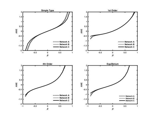
Figure 1. The Average Network Externality Comparison Between Equilibrium and Behavioral Models: Erdös-Rényi Graphs

Notes: Each line represents the average network externality (ANE) as a function of $\beta_{0}$. Each panel shows multiple lines representing ANE as we expand the graph from a subgraph of agents within distance $k$ from the agent 1. (Networks A, B, and C correspond to networks with $k=3,4,5$ from a small graph to a large one.) The figures show that the ANE is stable across different networks, and that the ANE from the behavioral model converges to that from the equilibrium model as the order of sophistication becomes higher.

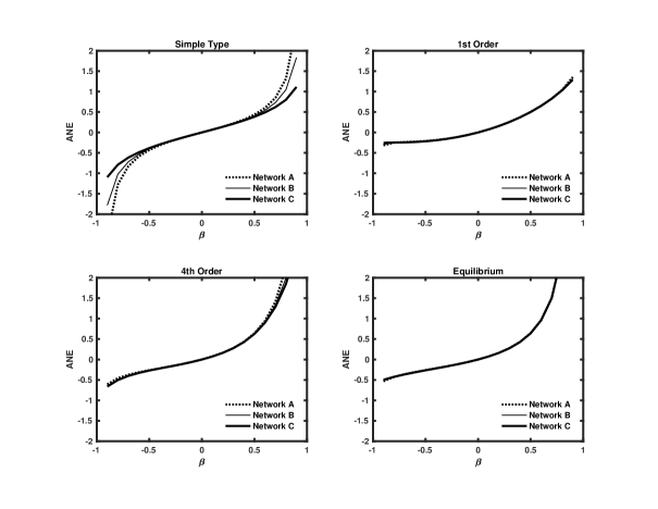
Figure 2. The Average Network Externality Comparison Between Equilibrium and Behavioral Models: Barabási-Albert Graphs

Notes: Each line represents the average network externality (ANE) as a function of $\beta_{0}$. Each panel shows multiple lines representing ANE as we expand the graph from a subgraph of agents within distance $k$ from the agent 1. (Networks A, B, and C correspond to networks with $k=2,3,4$ from a small graph to a large one.)

The ANEs from the equilibrium strategies from game $\Gamma_{\infty}$, and the behavioral strategies from games $\Gamma_{m}$ as $m$ becomes higher are shown in Figures 1 and 2. First, as $m$ becomes larger, the ANEs from $\Gamma_{\infty}$ and those from $\Gamma_{m}$ get closer, as predicted by Theorem 2.3. Furthermore, the ANEs from the behavioral model are similar to that from the equilibrium model especially when $\beta_{0}$ is between $-0.5$ and $0.5$. Finally, the network externalities from the games with simple type players are somewhat sensitive to the size of the networks when $\beta_{0}$ is very high or very low. This sensitivity is reduced substantially when we consider the game with first order sophisticated agents. Finally, network externality tends to be much higher for equilibrium models than the behavioral models when $\beta_{0}$ is high. Hence using our behavioral approach as a proxy for an equilibrium approach makes sense only when strategic interdependence is not too high.

3. Econometric Inference

3.1. General Overview

3.1.1. Partial Observation of Interactions

A large network data set is often obtained through a non-random sampling process. (See e.g. Kolaczyk:09:SAND.) The actual sampling process of network data is often unknown to the researcher. Our approach of empirical modeling can be useful in a situation where only a fraction of the players are observed through a certain non-random sampling scheme that is not precisely known to the researcher. In this section, we make explicit the data requirements for the econometrician and propose inference procedures. We mainly focus on the game where all the players in the game are of simple type. We develop inference for games with agents of first-order sophisticated type in the Supplemental Note.

Suppose that the original game of interactions consists of a large number of agents whose set we denote by $N$. Let the set of players be on a payoff graph $G_{P}$ and an information graph $G_{I}$, facing the strategic environment as described in the preceding section. Denote the best response as an observed dependent variable $Y_{i}$: for $i\in N$,

$$Y_{i}=s_{i}^{[0]}(\mathcal{I}_{i,0}),$$

where the sharable type $\tau_{i}$ is specified as:

(3.1) $$\tau_{i}=X_{i}^{\prime}\rho_{0}+\varepsilon_{i},$$

and $X_{i}$ is a $d$-dimensional vector of covariates pertaining to agent $i$ observed by the econometrician, $\rho_{0}\in\mathbf{R}^{d}$ is a coefficient vector, and $\varepsilon_{i}$ is unobserved heterogeneity. The covariate $X_{i}$ can contain $G_{P}$-neighborhood averages of individual covariates. Let us make the following additional assumption on this original large game. Let us first define

$$\mathcal{F}=\sigma(X,G_{P},G_{I})\vee\mathcal{C},$$

i.e., the $\sigma$-field generated by $X=(X_{i})_{i\in N}$, $G_{P}$, $G_{I}$ and $\mathcal{C}$ is a given common shock which is to be explained below.

Assumption 3.1.

(i) $\varepsilon_{i}$’s and $\eta_{i}$’s are conditionally i.i.d. across $i$’s given $\mathcal{F}$.

(ii) $\{\varepsilon_{i}\}_{i=1}^{n}$ and $\{\eta_{i}\}_{i=1}^{n}$ are conditionally independent given $\mathcal{F}$.

(iii) For each $i\in N$, $\mathbf{E}[\varepsilon_{i}|\mathcal{F}]=0$ and $\mathbf{E}[\eta_{i}|\mathcal{F}]=0$.

Condition (i) excludes pre-existing cross-sectional dependence of unobserved heterogeneity in the payoffs once conditioned in $\mathcal{F}$. This condition implies that conditional on $\mathcal{F}$, the cross-sectional dependence of observed actions is due solely to the information sharing among the agents. Condition (ii) requires that conditional on $\mathcal{F}$, the unobserved payoff heterogeneities observed by other players and those that are private are independent. Condition (iii) excludes endogenous formation of $G_{P}$ or $G_{I}$, because the condition requires that the unobserved type components $\varepsilon_{i}$ and $\eta_{i}$ be conditionally mean independent of these graphs, given $X=(X_{i})_{i\in N}$ and $\mathcal{C}$. However, the condition does not exclude the possibility that $G_{P}$ and $G_{I}$ are exogenously formed based on $(X,\mathcal{C})$. For example, suppose that $ij\in E_{P}$ if and only if

$$f_{ij}(X_{i},X_{j},a_{i},a_{j},u_{ij})\geq 0,$$

where $a_{i}$ represents degree heterogeneity, $u_{ij}$’s errors, and $f_{ij}$ a given nonstochastic function. In this set-up, the econometrician does not observe $a_{i}$’s or $u_{ij}$’s. This nests the dyadic regression model of Graham:17:Eca as a special case. Condition (iii) accommodates such a set-up, as long as $\{a_{i}\}_{i=1}^{n}$ and $\{u_{ij}\}_{i,j=1}^{n}$ are conditionally independent of $\{\varepsilon_{i}\}_{i=1}^{n}$ and $\{\eta_{i}\}_{i=1}^{n}$ given $X$. One simply has to take $\mathcal{C}$ to contain $a_{i}$’s and $u_{ij}$’s.

The econometrician observes only a subset $N^{*}\subset N$ of agents and part of $G_{P}$ through a potentially stochastic sampling process of unknown form. We assume for simplicity that $n^{*}\equiv|N^{*}|$ is nonstochastic. This assumption is satisfied, for example, if one collects the data for agents with predetermined sample size $n^{*}$. We assume that though being a small fraction of $N$, the set $N^{*}$ is still a large set justifying our asymptotic framework that sends $n^{*}$ to infinity. Most importantly, constituting only a small fraction of $N$, the observed sample $N^{*}$ of agents induces a payoff subgraph which one has no reason to view as “approximating” or “similar to” the original payoff graph $G_{P}$. Let us make precise the data requirements.

Condition A: The stochastic elements of the sampling process are conditionally independent of $\{(\tau_{i},\eta_{i})^{\prime}\}_{i\in N}$ given $\mathcal{F}$.

Condition B: For each $i\in N^{*}$, the econometrician observes $N_{P}(i)$ and $(Y_{i},X_{i})$, and for each $j\in N_{P}(i)$, the econometrician observes $|N_{P}(i)\cap N_{P}(j)|$, $n_{P}(j)$ and $X_{j}$.

Condition C: Either of the following two conditions is satisfied:

(a) For $i,j\in N^{*}$ such that $i\neq j$, $N_{P}(i)\cap N_{P}(j)=\varnothing$.

(b) For each agent $i\in N^{*}$, and for any agent $j\in N^{*}$ such that $N_{P}(i)\cap N_{P}(j)\neq\varnothing$, the econometrician observes $Y_{j}$, $|N_{P}(j)\cap N_{P}(k)|$, $n_{P}(k)$ and $X_{k}$ for all $k\in N_{P}(j)$.

Before we discuss the conditions, it is worth noting that these conditions are trivially satisfied when we observe the full payoff graph $G_{P}$ and $N^{*}=N$. Condition A is satisfied, for example, if the sampling process is based on observed characteristics $X$ and some characteristics of the strategic environment that is commonly observed by all the players. This condition is violated if the sampling is based on the outcomes $Y_{i}$’s or unobserved payoff-relevant signals such as $\varepsilon_{i}$ or $\eta_{i}$. Condition B essentially requires that in the data set, we observe $(Y_{i},X_{i})$ of many agents $i$, and for each $G_{P}$-neighbor $j$ of agent $i$, observe the number of the agents who are common $G_{P}$-neighbors of $i$ and $j$ and the size of $G_{P}$-neighborhood of $j$ along with the observed characteristics $X_{j}$. As for a $G_{P}$-neighbor $j$ of agent $i\in N^{*}$, this condition does not require that the agent $j$’s action $Y_{j}$ or the full set of his $G_{P}$-neighbors are observed. Condition C(a) is typically satisfied when an initial sample of agents is randomly selected from a much larger set of agents so that no two agents have overlapping $G_{P}$-neighbors in the sample, and then their $G_{P}$ neighbors are selected for each agent in the sample to constitute $N^{*}$. In practice for use in inference, one can take the set $N^{*}$ to include only those agents that satisfy Conditions A-C as long as $N^{*}$ thereof is still large and the selection is based only on $(X,G_{P})$. One can simply use only those agents whose $G_{P}$-neighborhoods are not overlapping, as long as there are many such agents in the data.

3.1.2. Moment Conditions

In order to introduce inference procedures for $\beta_{0}$ and other payoff parameters, let us define for $i\in N$,

(3.2) $$Z_{i}=\left(1+\frac{\beta_{0}^{2}\overline{\lambda}_{i}}{n_{P}(i)-\beta_{0}^{2}\overline{\lambda}_{i}}\right)\left(X_{i}+\frac{\beta_{0}}{n_{P}(i)}\sum_{j\in N_{P}(i)}\lambda_{ij}X_{j}\right).$$

(Note that $Z_{i}$ relies on $\beta_{0}$ although it is suppressed from notation for simplicity as we do frequently below for other quantities.) By Theorem 2.1 and (3.1), we can write

(3.3) $$Y_{i}=Z_{i}^{\prime}\rho_{0}+v_{i},$$

where

$$v_{i}=\left(1+\frac{\beta_{0}^{2}\overline{\lambda}_{i}}{n_{P}(i)-\beta_{0}^{2}\overline{\lambda}_{i}}\right)\left(\varepsilon_{i}+\frac{\beta_{0}}{n_{P}(i)}\sum_{j\in N_{P}(i)}\lambda_{ij}\varepsilon_{j}\right)+\eta_{i}.$$

Note that the observed actions $Y_{i}$ are cross-sectionally dependent (conditional on $\mathcal{F}$) due to information sharing on unobservables $\varepsilon_{i}$.

Suppose that $\varphi_{i}$ is $M\times 1$ vector of instrumental variables (which potentially depend on $\beta_{0}$) with $M>d$ such that for all $i\in N$,

(3.4) $$\mathbf{E}[v_{i}\varphi_{i}]=0.$$

Note that the orthogonality condition above holds for any $\varphi_{i}$ as long as for each $i\in N$, $\varphi_{i}$ is $\mathcal{F}$-measurable, i.e., once $\mathcal{F}$ is realized, there is no extra randomness in $\varphi_{i}$. This is the case, for example, when $\varphi_{i}$ is a function of $X=(X_{i})_{i\in N}$ and $G_{P}$.

While the asymptotic validity of our inference procedure admits a wide range of choices for $\varphi_{i}$’s, one needs to choose them with care to obtain sharp inference on the payoff parameters. Especially, it is important to consider instrumental variables which involve the characteristics of $G_{P}$-neighbors to obtain sharp inference on payoff externality parameter $\beta_{0}$. This is because the cross-sectional dependence of observations carries substantial information for strategic interdependence among agents.

3.1.3. Local Identification

It is not hard to see that under regularity conditions (such as those preventing multicollinearity in $Z_{i}$), $\rho_{0}$ is identified up to $\beta_{0}$. However, the moment function in (3.4) is nonlinear in $\beta_{0}$, and hence even local identification of $\beta_{0}$ is not guaranteed unless we impose further assumptions. Here we provide conditions for local identification, but for inference we propose later, we pursue asymptotically valid inference allowing the parameters to be only partially identified.

Let $\theta\equiv[\beta,\rho^{\prime}]^{\prime}$ and write $v_{i}(\theta)=Y_{i}-Z_{i}^{\prime}(\beta)\rho$, where $Z_{i}(\beta)$ is the same as $Z_{i}$ except that $\beta_{0}$ is replaced by $\beta$. Let $\Theta$ be the parameter space for $\theta_{0}$.

Assumption 3.2.

(i) For all $i=1,...,n$, $\varphi_{i}$ does not depend on $\theta\in\Theta$, and the parameter space $\Theta$ is compact, and $\beta\in[-1+\nu,1-\nu]$ for all $\beta$ such that $[\beta,\rho^{\prime}]^{\prime}\in\Theta$, for some small $\nu>0$.

(ii) There exists $C>0$ such that for all $n\geq 1$,

$$\frac{1}{n}\sum_{i=1}^{n}\mathbf{E}\left[\left.\|X_{i,n}\|^{4}+\frac{1}{n_{P}(i)}\sum_{j\in N_{P}(i)}\|X_{j,1}\|^{4}\right|G_{P}\right]+\frac{1}{n}\sum_{i=1}^{n}\mathbf{E}\left[\|\varphi_{i}\|^{4}|G_{P}\right]<C.$$

(iii) There exists $c>0$ such that the minimum eigenvalue of the matrix

$$\sum_{m=1}^{M}\left(\frac{1}{n}\sum_{i=1}^{n}H_{i,m}(\theta_{0})\right)\left(\frac{1}{n}\sum_{i=1}^{n}H_{i,m}(\theta_{0})\right)^{\prime}$$

is bounded from below by $c$ for all $n\geq 2$, where

$$H_{i,m}(\theta)\equiv\mathbf{E}\left[\left.\left[\binom{\partial v_{i}(\theta)/\partial\beta}{-Z_{i}(\beta)}\varphi_{i,m}\right]\right|G_{P}\right],$$

and $\varphi_{i,m}$ is the $m$-th entry of $\varphi_{i}$.

(iv) $\max_{i\in N}n_{P}^{2}(i)/\sqrt{n}\rightarrow 0$, as $n\rightarrow\infty$.

Assumption 3.2(i) in regards to $\varphi_{i}$ simplifies the identification arguments and is satisfied when the “instruments” $\varphi_{i}$ consist only of observed variables. Assumption 3.2(ii) is a moment condition for the covariates. Assumption 3.2(iii) is a nontrivial condition and is violated if the parameter space for $\rho_{0}$ includes zero, because we have $\partial v_{i}(\beta,0)/\partial\beta=0$. Thus this assumption requires the researcher to know that the true parameter $\rho_{0}$ is away from zero. Assumption 3.2(iv) is a mild condition that requires that the payoff graph $G_{P}$ is not overly dense.

Under this assumption, in combination with the conditions of Theorem 2.1, we can show that $\theta_{0}$ is locally identified (i.e., consistently estimable over a neighborhood of $\theta_{0}$.)

Theorem 3.1.

Suppose that Assumption 3.2 and the conditions of Theorem 2.1 hold. Then, there exists $\varepsilon>0$ such that if $\Theta=\overline{B}(\theta_{0};\varepsilon)$, $\theta_{0}$ is consistently estimable, where $B(\theta_{0};\varepsilon)$ is the $\varepsilon$-neighborhood of $\theta_{0}$ and $\overline{B}(\theta_{0};\varepsilon)$ is its closure.

Since consistent estimability of $\theta_{0}$ requires that $\rho_{0}$ be away from zero, it is expected that as $\rho_{0}$ gets close to zero, $\beta_{0}$ is only “weakly (locally) identified”. As a researcher is rarely a priori certain that $\rho_{0}$ is away from zero, we pursue inference that does not require this.

3.1.4. Estimation and Inference

We first estimate $\rho_{0}$ assuming knowledge of $\beta_{0}$. Define

$$S_{\varphi\varphi}=\varphi^{\prime}\varphi/n^{*},\text{ and }\tilde{\varphi}=\varphi S^{-1/2}_{\varphi\varphi},$$

where $\varphi$ is an $n^{*}\times M$ matrix whose $i$-th row is given by $\varphi_{i}^{\prime}$, $i\in N^{*}$. Define

(3.5) $$\Lambda=\frac{1}{n^{*}}\sum_{i\in N^{*}}\sum_{j\in N^{*}}\mathbf{E}[v_{i}v_{j}|\mathcal{F}]\tilde{\varphi}_{i}\tilde{\varphi}_{j}^{\prime},$$

where $\tilde{\varphi}_{i}$ represents the transpose of the $i$-th row of $\tilde{\varphi}$, and let $\hat{\Lambda}$ be a consistent estimator of $\Lambda$. (We will explain how we construct this estimator in Section 3.1.7 below.) Define

$$S_{Z\tilde{\varphi}}=Z^{\prime}\tilde{\varphi}/n^{*},\text{ and }S_{\tilde{\varphi}y}=\tilde{\varphi}^{\prime}y/n^{*},$$

where $Z$ is an $n^{*}\times d$ matrix whose $i$-th row is given by $Z_{i}^{\prime}$ and $y$ is an $n^{*}\times 1$ vector whose $i$-th entry is given by $Y_{i}$, $i\in N^{*}$. Then we estimate

(3.6) $$\hat{\rho}=\left[S_{Z\tilde{\varphi}}\hat{\Lambda}^{-1}S_{Z\tilde{\varphi}}^{\prime}\right]^{-1}S_{Z\tilde{\varphi}}\hat{\Lambda}^{-1}S_{\tilde{\varphi}y}.$$

Using this estimator, we construct a vector of residuals $\hat{v}=[\hat{v}_{i}]_{i\in N^{*}}$, where

(3.7) $$\hat{v}_{i}=Y_{i}-Z_{i}^{\prime}\hat{\rho}.$$

Finally, we form a profiled test statistic as follows:

(3.8) $$\quad\quad\quad T(\beta_{0})=\frac{\hat{v}^{\prime}\tilde{\varphi}\hat{\Lambda}^{-1}\tilde{\varphi}^{\prime}\hat{v}}{n^{*}},$$

making it explicit that the test statistic depends on $\beta_{0}$. Later we show that

$$T(\beta_{0})\rightarrow_{d}\chi_{M-d}^{2},\text{ as }n^{*}\rightarrow\infty,$$

where $\chi_{M-d}^{2}$ denotes the $\chi^{2}$ distribution with degree of freedom $M-d$. Let $C_{1-\alpha}^{\beta}$ be the $(1-\alpha)100$% confidence set for $\beta_{0}$ defined as

$$C_{1-\alpha}^{\beta}\equiv\{\beta\in(-1,1):T(\beta)\leq c_{1-\alpha}\},$$

where $T(\beta)$ is computed as $T(\beta_{0})$ with $\beta_{0}$ replaced by $\beta$ and the critical value $c_{1-\alpha}$ is the $(1-\alpha)$-quantile of $\chi_{M-d}^{2}$.

Let us now construct a confidence set for $\rho_{0}$. First, we establish that under regularity conditions,

$$\sqrt{n^{*}}\hat{V}^{-1/2}(\hat{\rho}-\rho_{0})\rightarrow_{d}N(0,I_{d}),$$

as $n^{*}\rightarrow\infty$, where

$$\hat{V}=\left[S_{Z\tilde{\varphi}}\hat{\Lambda}^{-1}S_{Z\tilde{\varphi}}^{\prime}\right]^{-1}.$$

(See Section 3.2 below for conditions and formal results.) Using this estimator $\hat{\rho}$, we can construct a $(1-\alpha)100\%$ confidence interval for $a^{\prime}\rho_{0}$ for any non-zero vector $a$. For this define

$$\hat{\sigma}^{2}(a)=a^{\prime}\hat{V}a.$$

Let $z_{1-(\alpha/4)}$ be the $(1-(\alpha/4))$-percentile of $N(0,1)$. Define for a vector $a$ with the same dimension as $\rho$,

$$C_{1-(\alpha/2)}^{\rho}(\beta_{0},a)=\left[a^{\prime}\hat{\rho}-\frac{z_{1-(\alpha/4)}\hat{\sigma}(a)}{\sqrt{n}},a^{\prime}\hat{\rho}+\frac{z_{1-(\alpha/4)}\hat{\sigma}(a)}{\sqrt{n}}\right].$$

Then the confidence set for $a^{\prime}\rho$ is given by

$$C_{1-\alpha}^{\rho}(a)=\bigcup_{\beta\in C_{1-(\alpha/2)}^{\beta}}C_{1-(\alpha/2)}^{\rho}(\beta,a).$$

Notice that since $\beta$ runs in $(-1,1)$ and the estimator $\hat{\rho}$ has an explicit form, the confidence interval is not computationally costly to construct in general.

Often the eventual parameter of interest is one that captures how strongly the agents’s decisions are interdependent through the network. For this, we can use the average network externality (ANE) introduced in (2.13). Let $s_{i}^{[0]}(\mathcal{I}_{i,0})$ be the best response of agent $i$ having information set $\mathcal{I}_{i}$. Then the ANE with respect to $X_{i,r}$ (where $X_{i,r}$ represents the $r$-th entry of $X_{i}$) is given by $\theta_{1}(\beta_{0},\rho_{0,r})$, where

$$\theta_{1}(\beta_{0},\rho_{0,r}) = \frac{1}{n^{*}}\sum_{i\in N^{*}}\sum_{j\in N_{P}(i)}\frac{\partial s_{i}^{[0]}(\mathcal{I}_{i,0})}{\partial x_{j,r}}$$

$$= \frac{1}{n^{*}}\sum_{i\in N^{*}}\sum_{j\in N_{P}(i)}\frac{\beta_{0}\lambda_{ij}}{n_{P}(i)}\left(1+\frac{\beta_{0}^{2}\overline{\lambda}_{i}}{n_{P}(i)-\beta_{0}^{2}\overline{\lambda}_{i}}\right)\rho_{0,r},$$

and $\rho_{0,r}$ denotes the $r$-th entry of $\rho_{0}$. See (2.8). Thus the confidence interval for $\theta_{1}(\beta_{0},\rho_{0,r})$ can be constructed from the confidence interval for $\beta_{0}$ and $\rho_{0}$ as follows:

(3.9) $$C^{\theta_{1}}_{1-\alpha}=\left\{\theta_{1}(\beta,\rho_{r}):\beta\in C^{\beta}_{1-\alpha/2},\text{ and }\rho_{r}\in C^{\rho_{r}}_{1-\alpha/2}\right\},$$

where $C^{\beta}_{1-\alpha/2}$ and $C^{\rho_{r}}_{1-\alpha/2}$ denote the $(1-\alpha/2)100\%$ confidence intervals for $\beta_{0}$ and $\rho_{0,r}$ respectively.

3.1.5. Downweighting Players with High Degree Centrality

When there are players who are linked to many other players in $G_{P}$, the graph $G_{P}$ tends to be denser, and it becomes difficult to obtain good variance estimators that perform stably in finite samples. (In particular, obtaining an estimator of $\Lambda$ in (3.5) which performs well in finite samples can be difficult.) To remedy this situation, this paper proposes a downweighting of those players with high degree centrality in $G_{P}$. More specifically, in choosing an instrument vector $\varphi_{i}$, we may consider the following:

(3.10) $$\varphi_{i}(X)=\frac{1}{\sqrt{\overline{n}_{P}(i)}}g_{i}(X),$$

where $g_{i}(X)$ is a function of $X$. This choice of $\varphi_{i}$ downweights players $i$ who have a large $G_{P}$-neighborhood. Thus we rely less on the variations of the characteristics of those players who have many neighbors in $G_{P}$.

Downweighting agents too heavily may hurt the power of inference because the actions of agents with high centrality contain information about the parameter of interest through the moment restrictions. On the other hand, downweighting them too lightly may hurt the finite sample stability of inference due to strong cross-sectional dependence they cause to the observations. Since a model with agents of higher-order sophisticated type results in observations with more extensive cross-sectional dependence, the role of downweighting can be important for finite sample stability of inference in such a model.

3.1.6. Comparison with Linear-in-Means Models

Let us compare our model with a linear-in-means model used in the literature, which is specified as follows:

(3.11) $$Y_{i}=X_{i,1}^{\prime}\gamma_{0}+\overline{X}_{i,2}^{\prime}\delta_{0}+\beta_{0}\mu_{i}^{e}(\overline{Y}_{i})+v_{i},$$

where $\mu_{i}^{e}(\overline{Y}_{i})$ denotes the player $i$’s expectation of $\overline{Y}_{i}$, and

$$\overline{Y}_{i}=\frac{1}{n_{P}(i)}\sum_{j\in N_{P}(i)}Y_{j}\text{ and }\overline{X}_{i,2}=\frac{1}{n_{P}(i)}\sum_{j\in N_{P}(i)}X_{j,2}.$$

The literature assumes rational expectations by equating $\mu_{i}^{e}(\overline{Y}_{i})$ to $\mathbf{E}[\overline{Y}_{i}|\mathcal{I}_{i}]$, and then proceeds to identification analysis of parameters $\gamma$, $\delta_{0}$ and $\beta_{0}$. For actual inference, one needs to use an estimated version of $\mathbf{E}[\overline{Y}_{i}|\mathcal{I}_{i}]$. One standard way in the literature is to replace it by $\overline{Y}_{i}$ so that we have

$$Y_{i}=X_{i,1}^{\prime}\gamma_{0}+\overline{X}_{i,2}^{\prime}\delta_{0}+\beta_{0}\overline{Y}_{i}+\tilde{v}_{i},$$

where $\tilde{v}_{i}$ is an error term defined as $\tilde{v}_{i}=\beta_{0}(\mathbf{E}[\overline{Y}_{i}|\mathcal{I}_{i}]-\overline{Y}_{i})+v_{i}$. The complexity arises due to the presence of $\overline{Y}_{i}$ which is an endogneous variable that is involved in the error term $\tilde{v}_{i}$.

As for dealing with endogeneity, there are two kinds of instrumental variables proposed in the literature. The first kind is a peers-of-peers type instrumental variable which is based on the observed characteristics of the neighbors of the neighbors. This strategy was proposed by Kelejian/Robinson:1993:PRS, Bramoulle/Djebbari/Fortin:09:JOE and DeGiorgi/Pellizzari/Redaelli:10:AEJ. The second kind of an instrumental variable is based on observed characteristics excluded from the group characteristics as instrumental variables. (See Brock/Durlauf:01:ReStud and Durlauf/Tanaka:08:EI.) However, finding such an instrumental variable in practice is not always a straightforward task in empirical research.

Our approach of empirical modeling is different in several aspects. Our modeling uses behavioral assumptions instead of rational expectations, and produces a reduced form for observed actions $Y_{i}$ from using best responses. This reduced form gives a rich set of testable implications and makes explicit the source of cross-sectional dependence in relation to the payoff graph. Our inference approach permits any nontrivial functions of $\mathcal{F}$ to serve as instrumental variables. Furthermore, one does not need to observe many independent interactions for inference.

3.1.7. Estimation of Asymptotic Covariance Matrix

One needs to find estimators $\hat{\Lambda}$ and $\hat{V}$ to perform inference. First, let us find an expression for their population versions. After some algebra, it is not hard to see that the population version (conditional on $\mathcal{F}$) of $\hat{V}$ is given by

(3.12) $$V=\left[S_{Z\tilde{\varphi}}\Lambda^{-1}S_{Z\tilde{\varphi}}^{\prime}\right]^{-1}.$$

For estimation, it suffices to estimate $\Lambda$ defined in (3.5). For this, we need to incorporate the cross-sectional dependence of the residuals $v_{i}$ properly. From the definition of $v_{i}$, it turns out that $v_{i}$ and $v_{j}$ can be correlated if $i$ and $j$ are connected indirectly through two edges in $G_{P}$. One may construct an estimator of $\Lambda$ that is similar to the HAC (Heteroskedasticity and Autocorrelation Consistent) estimator, simply by imposing the dependence structure and replacing $v_{i}$ by $\hat{v}_{i}$. However, this standard method can lead to conservative inference with unstable finite sample properties, especially when each player has many players connected through two edges. Instead, this paper proposes an alternative estimator of $\Lambda$ as follows. (See the Supplemental Note for more explanations for this estimator.)

Fixing a value for $\beta_{0}$, we first obtain a first-step estimator of $\rho$ as follows:

(3.13) $$\tilde{\rho}=\left[S_{Z\tilde{\varphi}}S_{Z\tilde{\varphi}}^{\prime}\right]^{-1}S_{Z\tilde{\varphi}}S_{\tilde{\varphi}y}.$$

(Compare this with (3.6).) Using this estimator, we construct a vector of residuals $\tilde{v}=[\tilde{v}_{i}]_{i\in N^{*}}$, where

(3.14) $$\tilde{v}_{i}=Y_{i}-Z_{i}^{\prime}\tilde{\rho}.$$

Then we define

$$\hat{\Lambda}_{1} = \frac{1}{n^{*}}\sum_{i\in N^{*}}\tilde{v}_{i}^{2}\tilde{\varphi}_{i}\tilde{\varphi}_{i}^{\prime},\text{ and }$$

$$\hat{\Lambda}_{2} = \frac{\hat{s}_{\varepsilon}}{n^{*}}\sum_{i\in N^{*}}\sum_{j\in N^{*}_{-i}:N_{P}(i)\cap N_{P}(j)\neq\varnothing}q_{\varepsilon,ij}\tilde{\varphi}_{i}\tilde{\varphi}_{j}^{\prime},$$

where

(3.15) $$\hat{s}_{\varepsilon}=\frac{\displaystyle\sum_{i\in N^{*}}\sum_{j\in N_{P}(i)\cap N^{*}}\tilde{v}_{i}\tilde{v}_{j}}{\displaystyle\sum_{i\in N^{*}}\sum_{j\in N_{P}(i)\cap N^{*}}q_{\varepsilon,ij}},$$

and

$$q_{\varepsilon,ij}=w_{ii}^{[0]}w_{jj}^{[0]}\left(\frac{\lambda_{ji}1\{i\in N_{P}(j)\}}{n_{P}(j)}+\frac{\lambda_{ij}1\{j\in N_{P}(i)\}}{n_{P}(i)}+\frac{\beta_{0}}{n_{P}(i)n_{P}(j)}\sum_{k\in N_{P}(i)\cap N_{P}(j)}\lambda_{ik}\lambda_{jk}\right).$$

(Note that the quantity $q_{\varepsilon,ij}$ can be evaluated once $\beta_{0}$ is fixed.) We construct an estimator of $\Lambda$ as follows:

$$\hat{\Lambda}=\hat{\Lambda}_{1}+\hat{\Lambda}_{2}.$$

Using $\hat{\Lambda}$, we take the estimator for the covariance matrix $V$ to be

(3.16) $$\hat{V}=\left[S_{Z\tilde{\varphi}}\hat{\Lambda}^{-1}S_{Z\tilde{\varphi}}^{\prime}\right]^{-1}.$$

3.2. Asymptotic Theory

In this section, we present the assumptions and formal results of asymptotic inference. We introduce some technical conditions.

Assumption 3.3.

There exists $c>0$ such that for all $n^{*}\geq 1$, $\lambda_{\min}(S_{\varphi\varphi})\geq c$, $\lambda_{\min}(S_{Z\tilde{\varphi}}S_{Z\tilde{\varphi}}^{\prime})\geq c$, $\lambda_{\min}(S_{Z\tilde{\varphi}}\Lambda^{-1}S_{Z\tilde{\varphi}}^{\prime})\geq c$, $\lambda_{\min}(\Lambda)\geq c$, $\sigma_{\eta}^{2}>0$, and

$$\frac{1}{n^{*}}\sum_{i\in N^{*}}\frac{1}{n_{P}(i)}\sum_{j\in N_{P}(i)\cap N^{*}}\lambda_{ij}>c,$$

where $\lambda_{\min}(A)$ for a symmetric matrix $A$ denotes the minimum eigenvalue of $A$.

Assumption 3.4.

There exists a constant $C>0$ such that for all $n^{*}\geq 1$,

$$\max_{i\in N^{\circ}}||X_{i}||+\max_{i\in N^{\circ}}||\tilde{\varphi}_{i}||\leq C$$

and $\mathbf{E}[\varepsilon_{i}^{4}|\mathcal{F}]+\mathbf{E}[\eta_{i}^{4}|\mathcal{F}]<C$, where $n^{\circ}=|N^{\circ}|$ and

$$N^{\circ}=\bigcup_{i\in N^{*}}\overline{N}_{P}(i).$$

Assumption 3.3 is used to ensure that the asymptotic distribution is nondegenerate. This regularity condition is reasonable, because an asymptotic scheme that gives a degenerate distribution would not be adequate for approximating a finite sample, nondegenerate distribution of an estimator. Assumption 3.4 can be weakened at the expense of added complexity in the conditions and the proofs.

We introduce an assumption which requires the payoff graph to have a bounded degree over $i$ in the observed sample $N^{*}$.

Assumption 3.5.

There exists $C>0$ such that for all $n^{*}\geq 1$,

$$\max_{i\in N^{*}}|N_{P}(i)|\leq C.$$

We may relax the assumption to a weaker, yet more complex condition at the expense of longer proofs, but in our view, this relaxation does not give additional insights. When $N^{*}$ is large, one can remove very high-degree nodes to obtain stable inference. As such removal is solely based on the payoff graph $G_{P}$, the removal does not lead to any violation of the conditions in the paper.

The following theorem establishes the asymptotic validity of inference based on the best responses in Theorem 2.1, without using Assumption 3.2, i.e., without requiring local identification of $\theta_{0}$.

Theorem 3.2.

Suppose that the conditions of Theorem 2.1 and Assumptions 3.1 - 3.5 hold. Then,

$$T(\beta_{0})\rightarrow_{d}\chi^{2}_{M-d},\text{ and }\hat{V}^{-1/2}\sqrt{n^{*}}\left(\hat{\rho}-\rho_{0}\right)\rightarrow_{d}N(0,I_{d}),$$

as $n^{*}\rightarrow\infty$.

The theorem yields that the confidence sets for $\beta_{0}$ and $\rho_{0}$ that we proposed earlier are asymptotically valid. The proof of both theorems are found in the Supplemental Note. At the center of the asymptotic derivation is noting first that $v_{i}$’s have a conditional depenency graph in the sense that two sets $(v_{j})_{j\in A}$ and $(v_{j})_{j\in B}$ with $G_{P}$ neighborhoods of $A$ and $B$ nonoverlapping are conditionally independent given $\mathcal{F}$) and then applying the Central Limit Theorem for a sum of random variables that has a sparse conditional dependency graph. For the proof, we use a version of such a central limit theorem in Penrose:03:RandomGeometricGraphs. The sparsity of such a graph is ensured by the bounded degree assumption (3.5). (Note that we can relax this assumption by letting the maximum degree increase slowly with $n$, but as mentioned before, this relaxation does not add additional insights only lengthening the mathematical proofs.) The local dependence structure coming from the conditional dependency graph affects our inference through the estimated variance via the way $\hat{\Lambda}$ is constructed. If the payoff graph $G_{P}$ is not sparse enough, the asymptotic approximation in Theorem 3.2 may perform poorly in finite samples.

4. A Monte Carlo Simulation Study

4.1. Simulation Design

In this section, we investigate the finite sample properties of the asymptotic inference across various configurations of the payoff graph, $G_{P}$. (We present Monte Carlo simulation results for the game with the first-order sophisticated types in Appendix E in the Supplemental Note.) The payoff graphs are generated according to two models of random graph formation, which we call Specifications 1 and 2. Specification 1 uses the Barabási-Albert model of preferential attachment, with $m$ representing the number of edges each new node forms with existing nodes. The number $m$ is chosen from $\{1,2,3\}$. Specification 2 is the Erdös-Rényi random graph with probability $p=\lambda/n$, where $\lambda$ is also chosen from $\{1,2,3\}$. In Table 2, we report degree characteristics of the payoff graphs used in the simulation study.

For the simulations, we set the following:

$$\tau_{i} =X_{i}^{\prime}\rho_{0}+\varepsilon_{i},$$

where $\rho_{0}=(2,4,1,3,4)^{\prime}$ and $X_{i}=(X_{i,1},\overline{X}_{i,2})^{\prime}$, and

$$\overline{X}_{i,2}=\frac{1}{n_{P}(i)}\sum_{j\in N_{P}(i)}X_{j,2}.$$

We generate $Y_{i}$ from the best response function in Theorem 2.1 (or as in (3.3)). We set and $a$ to be a column of ones so that $a^{\prime}\rho_{0}=14$. The variables $\varepsilon$ and $\eta$ are drawn i.i.d. from $N(0,1)$. The first column of $X_{i,1}$ is a column of ones, while remaining columns of $X_{i,1}$ are drawn independently from $N(1,1)$. The columns of $X_{i,2}$ are drawn independently from $N(3,1)$.

For instruments, we use downweighting (3.10) as follows:

$$\varphi_{i}(X)=\frac{1}{\sqrt{\overline{n}_{P}(i)}}g_{i}(X),$$

where

$$g_{i}(X)=[\tilde{Z}_{i,1},X_{i,1}^{2},\overline{X}_{i,2}^{2},\overline{X}_{i,2}^{3}]^{\prime},$$

where we define

$$\tilde{Z}_{i,1}\equiv\frac{1}{n_{P}(i)}\sum_{j\in N_{P}(i)}\lambda_{ij}X_{j,1}.$$

While the instruments $X_{i,1}^{2},\overline{X}_{i,2}^{2},\overline{X}_{i,2}^{3}$ capture the nonlinear impact of $X_{i}$’s, the instrument $\tilde{Z}_{i,1}$ captures the cross-sectional dependence along the payoff graph. The use of this instrumental variable is crucial in obtaining a sharp inference for $\beta_{0}$. Note that since we have already concentrated out $\rho_{0}$ in forming the moment conditions, we cannot use linear combinations of $X_{i,1}$ and $\overline{X}_{i,2}$ as our instrumental variables. The nominal size in all the experiments is set at $\alpha=0.05$. The Monte Carlo simulation number is set to 5000.

Table 2. The Average and Maximum Degrees of Graphs in the Simulations

		Specification 1			Specification 2
$n$		$m=1$	$m=2$	$m=3$	$\lambda=1$	$\lambda=2$	$\lambda=3$
$500$	$d_{mx}$	17	21	30	5	8	11
	$d_{av}$	1.7600	3.2980	4.8340	0.9520	1.9360	2.9600
$1000$	$d_{mx}$	18	29	34	6	7	9
	$d_{av}$	1.8460	3.5240	5.2050	0.9960	1.9620	3.0020
5000	$d_{mx}$	32	78	70	7	10	11
	$d_{av}$	1.9308	3.7884	5.6466	0.9904	2.0032	3.0228

Notes: This table gives characteristics of the payoff graphs, $G_{P}$, used in the simulation study. $d_{av}$ and $d_{mx}$ represent the average and maximum degrees of the networks respectively; that is, $d_{av}\equiv\frac{1}{n}\sum_{i\in N}n_{P}(i)$ and $d_{mx}\equiv\max_{i\in N}n_{P}(i)$.

Table 3. The Empirical Coverage Probability and Average Length of Confidence Intervals for $\beta_{0}$ at 95% Nominal Level.

Coverage Probability
		Specification 1			Specification 2
$\beta_{0}$		$m=1$	$m=2$	$m=3$	$\lambda=1$	$\lambda=2$	$\lambda=3$
$-0.5$	$n=500$	0.9642	0.9580	0.9648	0.9686	0.9638	0.9622
	$n=1000$	0.9638	0.9634	0.9574	0.9650	0.9644	0.9604
	$n=5000$	0.9596	0.9560	0.9530	0.9704	0.9608	0.9596
$-0.3$	$n=500$	0.9540	0.9536	0.9612	0.9608	0.9546	0.9568
	$n=1000$	0.9566	0.9568	0.9566	0.9564	0.9578	0.9548
	$n=5000$	0.9534	0.9548	0.9542	0.9636	0.9568	0.9546
$0$	$n=500$	0.9504	0.9464	0.9554	0.9474	0.9478	0.9490
	$n=1000$	0.9486	0.9508	0.9514	0.9498	0.9510	0.9526
	$n=5000$	0.9440	0.9490	0.9546	0.9516	0.9482	0.9478
$0.3$	$n=500$	0.9548	0.9512	0.9584	0.9562	0.9552	0.9556
	$n=1000$	0.9600	0.9558	0.9524	0.9598	0.9592	0.9590
	$n=5000$	0.9524	0.9536	0.9574	0.9604	0.9544	0.9522
$0.5$	$n=500$	0.9648	0.9574	0.9618	0.9640	0.9610	0.9620
	$n=1000$	0.9630	0.9604	0.9534	0.9710	0.9648	0.9634
	$n=5000$	0.9564	0.9598	0.9612	0.9700	0.9632	0.9584
Average Length of CI
		Specification 1			Specification 2
$\beta_{0}$		$m=1$	$m=2$	$m=3$	$\lambda=1$	$\lambda=2$	$\lambda=3$
$-0.5$	$n=500$	0.0834	0.1307	0.1947	0.1089	0.0751	0.0750
	$n=1000$	0.0490	0.0794	0.1038	0.0630	0.0438	0.0463
	$n=5000$	0.0053	0.0203	0.0303	0.0108	0.0026	0.0024
$-0.3$	$n=500$	0.0799	0.1216	0.1639	0.1083	0.0865	0.0910
	$n=1000$	0.0464	0.0758	0.0990	0.0639	0.0519	0.0577
	$n=5000$	0.0034	0.0187	0.0296	0.0116	0.0060	0.0075
$0$	$n=500$	0.0785	0.1212	0.1572	0.1070	0.0970	0.1087
	$n=1000$	0.0452	0.0753	0.0996	0.0638	0.0597	0.0700
	$n=5000$	0.0024	0.0182	0.0298	0.0113	0.0106	0.0155
$0.3$	$n=500$	0.0713	0.1062	0.1384	0.0983	0.0685	0.0676
	$n=1000$	0.0404	0.0640	0.0872	0.0562	0.0389	0.0412
	$n=5000$	0.0017	0.0155	0.0262	0.0076	0.0015	0.0013
$0.5$	$n=500$	0.0495	0.0738	0.1085	0.0666	0.0289	0.0240
	$n=1000$	0.0252	0.0337	0.0657	0.0328	0.0089	0.0079
	$n=5000$	0.0001	0.0055	0.0147	0.0004	0.0000	0.0000

Notes: The first half of the table reports the empirical coverage probability of the asymptotic confidence interval for $\beta_{0}$ and the second half reports its average length. The simulated rejection probability at the true parameter is close to the nominal size of $\alpha=0.05$ and the average lengths decrease with $n$. The simulation number is $R=5000$.

Table 4. The Empirical Coverage Probability and Average Length of Confidence Intervals for $a^{\prime}\rho_{0}$ at 95% Nominal Level.

Coverage Probability
		Specification 1			Specification 2
$\beta_{0}$		$m=1$	$m=2$	$m=3$	$\lambda=1$	$\lambda=2$	$\lambda=3$
$-0.5$	$n=500$	0.9848	0.9802	0.9860	0.9862	0.9834	0.9740
	$n=1000$	0.9616	0.9610	0.9680	0.9682	0.9670	0.9596
	$n=5000$	0.9596	0.9548	0.9606	0.9706	0.9668	0.9614
$-0.3$	$n=500$	0.9802	0.9772	0.9858	0.9832	0.9826	0.9794
	$n=1000$	0.9620	0.9756	0.9796	0.9772	0.9682	0.9692
	$n=5000$	0.9544	0.9510	0.9562	0.9588	0.9568	0.9556
$0$	$n=500$	0.9740	0.9754	0.9868	0.9828	0.9792	0.9786
	$n=1000$	0.9668	0.9770	0.9798	0.9746	0.9738	0.9756
	$n=5000$	0.9430	0.9500	0.9524	0.9546	0.9496	0.9494
$0.3$	$n=500$	0.9804	0.9804	0.9866	0.9810	0.9778	0.9788
	$n=1000$	0.9698	0.9794	0.9812	0.9816	0.9718	0.9758
	$n=5000$	0.9476	0.9524	0.9546	0.9572	0.9536	0.9498
$0.5$	$n=500$	0.9824	0.9828	0.9858	0.9810	0.9722	0.9720
	$n=1000$	0.9724	0.9786	0.9826	0.9810	0.9596	0.9594
	$n=5000$	0.9552	0.9536	0.9596	0.9626	0.9596	0.9542
Average Length of CI
		Specification 1			Specification 2
$\beta_{0}$		$m=1$	$m=2$	$m=3$	$\lambda=1$	$\lambda=2$	$\lambda=3$
$-0.5$	$n=500$	5.4643	10.2562	17.4488	7.0549	5.6285	6.0639
	$n=1000$	3.3501	5.9311	8.1165	4.2270	3.4243	3.8800
	$n=5000$	0.7489	1.8254	2.4970	1.1165	0.6337	0.6588
$-0.3$	$n=500$	4.2511	6.8326	9.5995	5.6856	4.9154	5.4091
	$n=1000$	2.5915	4.3335	5.6775	3.4711	3.0685	3.5331
	$n=5000$	0.5297	1.3514	1.9123	0.9505	0.7346	0.8560
$0$	$n=500$	3.5812	5.3587	6.8508	4.7774	4.3760	4.8399
	$n=1000$	2.1797	3.4445	4.4160	2.9651	2.7944	3.2136
	$n=5000$	0.4238	1.0993	1.5392	0.8365	0.7964	0.9882
$0.3$	$n=500$	3.3664	4.5527	5.7822	4.4438	3.2458	3.1962
	$n=1000$	2.0559	2.8904	3.6607	2.6872	2.0100	2.1074
	$n=5000$	0.4072	0.9592	1.2989	0.6961	0.4399	0.4713
$0.5$	$n=500$	3.0230	4.1201	5.8780	3.7624	2.1350	1.9826
	$n=1000$	1.7684	2.1613	3.4957	2.1027	1.1718	1.2075
	$n=5000$	0.3576	0.6764	1.0002	0.3995	0.3723	0.4081

Notes: The true $a^{\prime}\rho_{0}$ is equal to 14. The first half of the table reports the empirical coverage probability of the asymptotic confidence interval and the second half its average length for $a^{\prime}\rho_{0}$. The empirical coverage probability of the confidence interval for $a^{\prime}\rho_{0}$ is generally conservative which is expected from the use of the Bonferroni approach. Nevertheless, the length of the confidence interval is reasonably small. The simulation number, $R$, is 5000.

4.2. Results

The finite sample performance of the asymptotic inference is shown in Tables 3 and 4. Overall, the simulation results illustrate good power and size properties for the asymptotic inference on $\beta_{0}$ and $a^{\prime}\rho_{0}$.

As for the size properties, the coverage probabilities of confidence intervals for $\beta_{0}$ are close to 95% nominal level, as shown in Table 3. The size properties are already good with $n=500$, and thus, show little improvement as $n$ increase to $5000$. The coverage probabilities of confidence intervals for $a^{\prime}\rho_{0}$ (as shown in Table 4) are a little conservative. This conservativeness is expected, given the fact that the interval is constructed using a Bonferroni approach. The conservativeness is alleviated as we increase the sample size.

As for the power properties, we consider the average length of the confidence intervals. The confidence intervals for $\beta_{0}$ are very short, with average length around 0.1 - 0.2 when $n=500$ and 0 - 0.03 when $n=5000$. As for $a^{\prime}\rho_{0}$, the average length of the confidence intervals is around 2 - 17 when $n=500$ and 0.4 - 2.5 when $n=5000$. Since $a^{\prime}\rho_{0}=14$, the average length shows good power properties of the inference.

5. Empirical Application: State Presence across Municipalities

5.1. Motivation and Background

State capacity (i.e., the capacity of a country to provide public goods, basic services, and the rule of law) can be limited for various reasons. (See e.g. Besley/Persson:09:AER and Gennaioli/Voth:15:REStud). A “weak state” may arise due to political corruption and clientelism, and result in spending inadequately on public goods (Acemoglu:05:JME), accommodating armed opponents of the government (Powell:13:QJE), and war (McBride/Milante/Skaperdas:11:JCE). Empirical evidence has shown how these weak states can persist from precolonial times, with higher state capacities apparently related to current level prosperity at the ethnic and national levels (Gennaioli/Rainer:07:JEG and Michalopoulos/Papaioannou:13:Eca).

Our empirical application is based on a recent study by Acemoglu/GarciaJimeno/Robinson:15:AER who investigate the local choices of state capacity in Colombia, using a model of a complete information game on an exogenously formed network. In their set-up, municipalities choose a level of spending on public goods and state presence (as measured by either the number of state employees or state agencies). Network externalities in a municipality’s choice exist because municipalities that are adjacent to one another can benefit from their neighbors’ choices of public goods provisions, such as increased security, infrastructure and bureaucratic connections. Thus, a municipality’s choice of state capacity can be thought of as a strategic decision on a geographic network.

It is not obvious that public good provision in one municipality leads to higher spending on public goods in neighboring municipalities. Some neighbors may free-ride and under-invest in state presence if they anticipate others will invest highly. Rent-seeking by municipal politicians would also limit the provision of public goods. On the other hand, economies of scale could lend to complementarities in state presence across neighboring municipalities.

In our study, we extend the model in Acemoglu/GarciaJimeno/Robinson:15:AER to an incomplete information game where information may be shared across municipalities. In particular, we do not assume that all municipalities know and observe all characteristics and decisions of the others. It seems reasonable that the decisions made across the country may not be observed or well known by those municipalities that are geographically remote.

5.2. Empirical Set-up

Let $y_{i}$ denote the state capacity in municipality $i$ (as measured by the log number of public employees in municipality $i$) and $G_{P}$ denote the geographic network, where an edge is defined on two municipalities that are geographically adjacent. We assume that $G_{P}$ is exogenously formed.

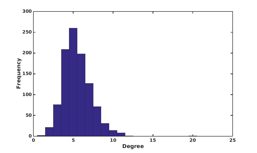
Figure 3. Degree Distribution of $G_{P}$

Notes: The figure presents the degree distribution of the graph $G_{P}$ used in the empirical specification. The average degree is 5.48, the maximum degree is 20, and the minimum degree is 1.

The degree distribution of $G_{P}$ is shown in Figure 3. We study the optimal choice of $y_{i}$, where $y_{i}$ leads to a larger prosperity $p_{i}$. Prosperity in municipality $i$ is modeled as:

(5.1) $$p_{i}=\left(\beta\bar{y}_{i}+x_{1,i}^{\prime}\gamma+\eta_{i}+\varepsilon_{i}+\varsigma^{D}_{i}\right)y_{i},$$

where $\varsigma^{D}_{i}$ is a district specific dummy variable, $\varepsilon_{i}$ and $\eta_{i}$ are our sharable and non-sharable private information, and $\overline{y}_{i}=\frac{1}{n_{P}(i)}\sum_{j\in N_{P}(i)}y_{j}.$ The term $x_{1,i}$ represents municipality characteristics. These include geographic characteristics, such as land quality, altitude, latitude, rainfall; and municipal characteristics, such as distance to highways, distance to royal roads and Colonial State Presence.

The welfare of a municipality is given by

(5.2) $$u_{i}(y_{i},y_{-i},\tau,\eta_{i})=p_{i}(y_{i},\bar{y}_{i},\tau,\eta_{i})-\frac{1}{2}y_{i}^{2},$$

where the second term refers to the cost of higher state presence, and the first term is the prosperity $p_{i}$.

We can rewrite the welfare of the municipality by substituting (5.1) into (5.2):

(5.3) $$u_{i}(y_{i},y_{-i},\tau,\eta_{i})=\left(\beta\bar{y}_{i}+x_{1,i}^{\prime}\gamma+\eta_{i}+\varepsilon_{i}+\varsigma^{D}_{i}\right)y_{i}-\frac{1}{2}y_{i}^{2}.$$

We assume that municipalities (or the mayor in charge), wishes to maximize welfare by choosing state presence, given their beliefs about the types of the other municipalities.

In our specification, we allow for incomplete information. This is reflected in the terms $\varepsilon_{i}$, $\eta_{i}$, which will be present in the best response function. The municipality, when choosing state presence $y_{i}$, will be able to observe $\varepsilon_{i}$ of its neighbors and will use its beliefs over the types of the others to generate its best response. The best response will follow the results from Theorem 2.1.

5.3. Model Specification

We closely follow Table 3 in Acemoglu/GarciaJimeno/Robinson:15:AER for the choice of specifications and variables. First, we will consider the model with simple types.

Throughout the specifications, we include longitude, latitude, surface area, elevation, annual rainfall, department fixed effects and a department capital dummy (all in $X_{1}$). We further consider the effect of variables distance to current highways, land quality and presence of rivers in the municipality.

For the choice of instruments, we consider two separate types of instruments. The first is the sum of neighbor values (across $G_{P}$) of the historical variables (denoted as $C_{i}$). The historical variables used are Total Crown Employees (also called Colonial State Officials), Distance to Royal Roads, Colonial State Agencies and Historical Population, as well as Colonial State Presence Index squared and Distance to Royal Roads squared. Using the latter two additionally sharpens inference. We also use the variable $\tilde{Z}_{i}=n_{P}(i)^{-1}\sum_{j\in N_{P}(i)}\lambda_{ij}X_{j,1}$ as part of the instrumental variables, which was shown to perform well in the Monte Carlo Simulations in Section 4. This variable captures cross sectional dependence as a crucial source of variation for inference on the strategic interactions. We use downweighting of our instruments as explained in a preceding section and rescale instruments by multiplying them by $S_{\varphi\varphi}^{-1/2}$.

5.4. Results

Table 5. State Presence and Networks Effects across Colombian Municipalities

		Outcome: The Number of State Employees
		Baseline	Distance to Highway	Land Quality	Rivers
		(1)	(2)	(3)	(4)
$\beta_{0}$		$[0.16,0.31]$	$[0.16,0.32]$	$[0.17,0.39]$	$[0.07,0.38]$
$dy_{i}/d(\text{\footnotesize colonial state}$		$[-0.060,0.003]$	$[-0.048,-0.001]$	$[-0.051,0.003]$	$[-0.034,0.009]$
$~{}\text{\footnotesize officials})$
Average
$dy_{i}/d(\text{\footnotesize colonial state}$		$[-1.323,4.051]$	$[-1.249,2.793]$	$[-0.972,3.545]$	$[-4.186,2.719]$
$~{}\text{\footnotesize agencies})$
Average
$dy_{i}/d(\text{\footnotesize distance to}$		$[-0.010,0.011]$	$[-0.009,0.011]$	$[-0.008,0.018]$	$[-0.010,0.013]$
$~{}\text{\footnotesize Royal Roads})$
$n$		1018	1018	1003	1003

Notes: Confidence sets for $\beta$ are presented in the table, obtained from inverting the test statistic $T(\beta)$ from Section 3 for First Order Sophisticated types, with confidence level of 95%. The critical values in the first row come from the asymptotic statistic. Downweighting is used. The average marginal effects for historical variables upon state capacity are also shown. The marginal effect of Colonial State Officials is equal to its $\gamma$ coefficient. The marginal effect for Distance to Royal Roads for municipality $i$ equals $\gamma_{Royal~{}Roads}+2*\gamma_{Royal~{}Roads^{2}}(Royal~{}Roads)_{i}$, where $\gamma_{Royal~{}Roads}$ is the $\gamma$ coefficient of its linear term, and $\gamma_{Royal~{}Roads^{2}}$ is the coefficient of its quadratic term, as this variable enters $X_{1}$as a quadratic form. The analogous expression holds for the variable Colonial State Agencies. We show the average marginal effect for these two variables. We then present the confidence set for these marginal effects, computed by the inference procedure on $a^{\prime}\gamma$ developed in Section 3. All specifications include controls of latitude, longitude, surface area, elevation, rainfall, as well as Department and Department capital dummies. Instruments are constructed from payoff neighbors’ sum of the $G_{P}$ neighbors values of the historical variables Total Crown Employees, Colonial State Agencies, Colonial State Agencies squared, population in 1843, distance to Royal Roads, distance to Royal Roads squared, together with the non-linear function $\tilde{Z}_{i}=n_{P}(i)^{-1}\sum_{j\in N_{P}(i)}\lambda_{ij}X_{j,1}$. Column (2) includes distance to current highway in $X_{1}$, Column (3) expands the specification of Column (2) by also including controls for land quality (share in each quality level). Column (4) controls for rivers in the municipality and land quality, in addition to those controls from Column (1). One can see that the results are very stable across specifications.

The results across a range of specifications are presented in Table 5. In these results, we see that the effect is statistically different than 0 and stable across specifications. It indicates that there is complementarity in the provision of public goods and state presence ($\beta>0$).

Let us compare our results to those in Acemoglu/GarciaJimeno/Robinson:15:AER. There, the authors report the average marginal effects over their weighted graph. The (weighted) average degree is 0.0329, so our results can be compared in an approximation, by considering 0.0329 $\hat{\beta}$.

In general, our estimates have the same sign and significance as those of Acemoglu/GarciaJimeno/Robinson:15:AER. Our estimates are in the range of [0.002, 0.013], after reweighting as mentioned before, somewhat comparable to theirs of [0.016, 0.022] (in the case of the outcome of the number of public employees, in Table 3). Hence, we find similar qualitative effects, although a smaller magnitude. Recall that our confidence set is built without assuming that $\beta_{0}$ is consistently estimable.

In Figure 4, we show the results of our estimated network externalities for the estimates from Table 5, for the importance of being a department capital. The average network externality (ANE) is computed as

$$\frac{1}{N}\sum_{i\in N}\sum_{j\in N_{P}(i)}\frac{\beta_{0}\hat{\gamma}_{dc}}{n_{P}(i)(1-\beta_{0}c_{ij})}\left(1+\frac{\beta_{0}^{2}\overline{\lambda}_{i}}{n_{P}(i)-\beta_{0}^{2}\overline{\lambda}_{i}}\right),$$

where $\hat{\gamma}_{dc}$ is the estimated parameter of the $X_{1}$ variable department capital. The parameter is defined in Section 3.1.4, and captures the average effect of a neighbor being a department capital. We construct a confidence interval as in (3.9).

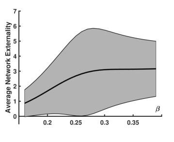
Figure 4. Average Network Externality from being a Department Capital

Notes: The figure presents the average network externalities from being a department capital. We use the estimated results from Column (3) in Table 5. This captures the externality for a municipality from being a department capital, which involves higher state presence and centralization of resources. This effect is not only the direct effect, but it also quantifies a reflection effect: neighbors of department capitals also benefit from it. The grey shaded area represents the 95% confidence interval for this ANE following the inference procedure developed in Section 3.

The figure shows that there is a strong and increasing network externality from being a department capital over the range of the confidence set of $\beta$. This indicates that the effect of being a capital has spillovers on other municipalities: since $\beta>0$, and one expects that department capitals have more state presence and resources, being a department capital yields increasing returns the stronger the complementarity.

6. Conclusion

This paper proposes a new approach of empirical modeling for interactions among many agents when the agents observe the types of their neighbors in a single large network. The main challenge arises from the fact that the information sharing relations are typically connected among a large number of players whereas the econometrician observes only a fraction of those agents. Using a behavioral model of belief formation, this paper produces an explicit form of best responses from which an asymptotic inference procedure for the payoff parameters is developed. As we showed in our paper, this explicit form gives a reduced form for the observed actions, and exhibits various intuitive features. For example, the best responses show that network externality is heterogeneous across agents depending on the relations of their payoff neighbors.

The main advantage of our paper’s approach is two-fold. First, the empirical modeling according to our approach accommodates a wide range of sampling processes. Such a feature is crucial because the econometrician rarely has precise knowledge about the actual sampling process through which data are generated. Second, the model can be used when only a fraction of the players are observed from a large connected network of agents. This can be quite useful as the econometrician typically does not observe the entire set of agents who interact with each other.

An interesting extension from this research is to consider the situation where the network formation is endogenous, i.e., the randomness of $G_{P}$ is correlated with the unobserved payoff heterogeneities of agents even after conditioning on the covariates. It is not trivial to extend our framework to this situation, because we need to explicitly consider the randomness of $G_{P}$ in relation to other variables instead of conditioning our inference on $G_{P}$ as we do in this paper. Such consideration should be properly made in the construction of moment conditions and the proposal of appropriate instrumental variables. We relegate this extension to future research.

econometrica matching_networks_A3

Supplemental Note to “Estimating Local Interactions Among Many Agents Who Observe Their Neighbors”

Nathan Canen, Jacob Schwartz, and Kyungchul Song

University of Houston, University of Haifa, and University of British Columbia

This supplemental note provides further details on Canen/Schwartz/Song:19:WP. This note consists of nine appendices. In Appendix A, we formally present a model of information sharing over time among many agents where the econometrician is interested in the estimation of local interactions in a particular decision problem. We explain how this extended model maps to the static model of the main paper. In Appendix B, we give the mathematical proofs of Theorems 2.1 and 2.2. We also provide details on the best response of a Bayesian decision maker and the result of coincidence of equilibrium strategies and behavioral strategies when the payoff graph has multiple disjoint complete subgraphs. In Appendix C, we explain how estimation of the asymptotic covariance matrix is motivated. Appendix D gives the proof of local identification (Theorem 3.1) and the asymptotic results (Theorem 3.2). Appendix E explains inference based on the model with first order sophisticated agents. The secion also provides the proof of the asymptotic validity of the proposed inference, and results from Monte Carlo simulation studies. Appendix F provides details on the model selection procedure between different games $\Gamma_{0}$ and $\Gamma_{1}$. Appendix G presents a proposal on testing for information sharing on unobservables. Appendix H gives the proofs of the results on the convergence of behavioral strategies to equilibrium strategies from game $\Gamma_{\infty}$ in Section 2.4.1. Appendix I gives the results from the empirical application using the game with first-order sophisticated agents.

Appendix A Information Sharing Among Many Agents Over Time

Information sharing among people takes place over time, and the econometrician usually observes part of these people as a snapshot in the process. The process involves information sharing, network formation and decision making. Agents can form a network and share information for various purposes. There is no reason to believe that each agent’s particular decision problem which is of interest to the econometrician is the single ultimate concern of the agents when they form a network at an earlier time. In this section, we provide an extended model of information sharing which fits the main set-up of the paper. The main idea is that people receive signals, form networks, and share information with their neighbors repeatedly. Then there is a decision making stage. The network formation (of either a payoff graph or an information graph) can be made, if not exclusively, in anticipation of the decision making later. However, as we will explain later in detail, our model assumes that when the agents form an information and a payoff graph, they do not observe other agents’ payoff relevant signals that are not observed by the econometrician. This is the precise sense in which the information and the payoff graph are exogenously formed.

Let us present a formal model of information sharing over time. Let $N$ be the set of a finite yet large number of players who share their type information over time recursively, where at each stage, players go through three steps sequentially: information graph formation, type realization and information sharing. Then at the final stage, players make a decision, maximizing their expected utilities.

At Stage 0, each agent $i\in N$ is endowed with signal $\mathcal{C}_{i,0}$. The signals can be correlated across agents in an arbitrary way. Then information sharing among agents happens recursively over time as follows starting from Stage $s=1$.

Stage s-1: (Information Graph Formation) Each player $i\in N$ receives signal $\mathcal{C}_{i,s-1}$. Using these signals, the players in $N$ form an information sharing network $G_{I,s-1}=(N,E_{I,s-1})$ among themselves, where $G_{I,s-1}=(N,E_{I,s-1})$ is a directed graph on $N$.

(Type Realization) Each player $i\in N$ is given his type vector $(\tau_{i,s-1}^{\prime},\eta_{i,s-1})^{\prime}$, where $\eta_{i,s-1}$ is a private type which player $i$ keeps to himself and $\tau_{i,s-1}$ a sharable type which is potentially observed by other agents.

(Information Sharing) Each player $i$ observes the sharable type $\tau_{j,s-1}$ of each player $j$ in his neighborhood in the information sharing network.

Stage s: (Information Graph Formation) Each player $i\in N$ receives signal $\mathcal{C}_{i,s}$ which contains part of $\mathcal{C}_{i,s-1}$ and part of the information about $G_{I,s-1}$ and $\tau_{j,s-1}$ with $j\in N_{I,s-1}(i)$. Using these signals, the players in $N$ form an information sharing network $G_{I,s}=(N,E_{I,s})$ among themselves, where $G_{I,s}=(N,E_{I,s})$ is a directed graph on $N$, and receives signal $\mathcal{C}_{i,s}$.

(Type Realization) Each player $i\in N$ is given his type vector $(\tau_{i,s}^{\prime},\eta_{i,s})^{\prime}$, where $\eta_{i,s}$ is a private type which player $i$ keeps to himself and $\tau_{i,s}$ a sharable type which is potentially observed by other agents.

(Information Sharing) Each player $i$ observes the sharable type $\tau_{j,s}$ of each player $j$ in his neighborhood in the information sharing network $G_{I,s}$.

The information sharing activities proceed up to Stage $S-1$. Then each agent faces a decision making problem.

Decision Stage: (Payoff Graph Formation) Each player $i\in N$ receives signal $\mathcal{C}_{i,S}$ which contains part of $\mathcal{C}_{i,S-1}$ and part of information about $G_{I,S-1}$ and $\tau_{j,S-1}$ with $j\in N_{I,S-1}(i)$. Using these signals, the players in $N$ form a payoff graph $G_{P}=(N,E_{P})$ among themselves, where $G_{I,S}=(N,E_{I,S})$ is a directed graph on $N$, and receives signal $\mathcal{C}_{i,S}$.

(Type Realization) Each player $i\in N$ is given his type vector $(\tau_{i,S}^{\prime},\eta_{i,S})^{\prime}$, where $\eta_{i,S}$ is a private type which player $i$ keeps to himself and $\tau_{i,S}$ a sharable type which is potentially observed by other agents.

(Information Sharing) Each player $i$ observes the sharable type $\tau_{j,S}$ of each player $j$ in his neighborhood in the information sharing network $G_{I,S}$.

(Decision) Each player $i$ makes a decision which maximizes his expected utility given his beliefs about other agents’ strategies using the information accumulated so far.

Now let us consider how this model of information sharing over time maps to our static local interactions model in our main paper. Our local interactions model captures the state where each player in $N$ faces the Decision Stage as follows. The information graph $G_{I}$ corresponds to $G_{I,S}$ and the payoff graph $G_{P}$ as described in Decision Stage above. The type vector $\tau_{i}$ and $\eta_{i}$ for each player $i\in N$ correspond to $\tau_{i,S}$ and $\eta_{i,S}$ as above. The signal $\mathcal{C}_{i}$ for each agent $i$ is defined to be

$$\mathcal{C}_{i}=\bigvee_{s=1}^{S}\mathcal{C}_{i,s},$$

where $\mathcal{A}_{1}\vee\mathcal{A}_{2}$ denotes the smallest $\sigma$-field that contains both $\mathcal{A}_{1}$ and $\mathcal{A}_{2}$. Therefore, each agent $i$’s signal $\mathcal{C}_{i}$ contains the information that has been accumulated so far. This information contains past information sharing experiences that have happened over time.

Observe that here we deliberately separate the information sharing stage and the decision stage. This is because people typically share information without necessarily anticipating the particular decision problem that the econometrician happens to later investigate.

Appendix B Best Responses

B.1. Proofs of Theorems 2.1- 2.2

Lemma B.1.

Suppose that $\beta_{0}\in(-1,1)$. Then, for any $i\in N$ such that $n_{P}(i)\geq 1$,

$$n_{P}(i)-\beta_{0}^{2}\overline{\lambda}_{i}\geq\frac{n_{P}(i)(n_{P}(i)+|\beta_{0}|)(1-|\beta_{0}|)}{n_{P}(i)(1-|\beta_{0}|)+|\beta_{0}|},$$

and

(B.1) $$0\leq w_{ii}^{[0]}\leq 1+\frac{\beta_{0}^{2}}{1-\beta_{0}^{2}},\text{ and }\left|w_{ij}^{[0]}\right|\leq\frac{|\beta_{0}|}{n_{P}(i)(1-|\beta_{0}|)}\left(1+\frac{\beta_{0}^{2}}{1-\beta_{0}^{2}}\right).$$

Proof: First, note that for any $j\in N_{P}(i)$,

(B.2) $$c_{ij}\leq\frac{n_{P}(i)-1}{n_{P}(i)}.$$

Hence

(B.3) $$\lambda_{ij}\leq\frac{n_{P}(i)}{n_{P}(i)-|\beta_{0}|(n_{P}(i)-1)}=\frac{n_{P}(i)}{n_{P}(i)(1-|\beta_{0}|)+|\beta_{0}|}.$$

Therefore,

(B.4) $$\overline{\lambda}_{i}\leq\frac{n_{P}(i)}{n_{P}(i)(1-|\beta_{0}|)+|\beta_{0}|}.$$

Now, we find that

$$n_{P}(i)-\beta_{0}^{2}\overline{\lambda}_{i} \geq n_{P}(i)-\frac{\beta_{0}^{2}n_{P}(i)}{n_{P}(i)(1-|\beta_{0}|)+|\beta_{0}|}$$

$$= \frac{n_{P}(i)(n_{P}(i)+|\beta_{0}|)(1-|\beta_{0}|)}{n_{P}(i)(1-|\beta_{0}|)+|\beta_{0}|}.$$

This gives the desired lower bound for $n_{P}(i)-\beta_{0}^{2}\overline{\lambda}_{i}$.

Let us turn to $w_{ii}^{[0]}$. Since $\lambda_{ij}\geq 0$, we have $w_{ii}^{[0]}\geq 0$ by the previous bound. As for its upper bound, from (B.4), we have

$$w_{ii}^{[0]}\leq 1+\frac{\beta_{0}^{2}}{(n_{P}(i)+|\beta_{0}|)(1-|\beta_{0}|)}\leq 1+\frac{\beta_{0}^{2}}{1-\beta_{0}^{2}},$$

because $n_{P}(i)\geq 1$. Finally, as for $w_{ij}^{[0]}$, it suffices to note that by (B.2),

$$0\leq\lambda_{ij}\leq\frac{1}{1-|\beta_{0}|}.$$

$\blacksquare$

Proof of Theorem 2.1: The case of $n_{P}(i)=0$ is trivial. Let us assume that $n_{P}(i)\geq 1$. From the optimization of agent $i$,

(B.5) $$s_{i}^{[0]}(\mathcal{I}_{i,0})=\tau_{i}+\beta_{0}\left(\frac{1}{n_{P}(i)}\sum_{k\in N_{P}(i)}\sum_{j\in\overline{N}_{P}(k)}w_{kj}^{i}\tau_{j}\right)+\eta_{i}.$$

Reorganizing the terms, we have

$$s_{i}^{[0]}(\mathcal{I}_{i,0}) = \left(1+\frac{\beta_{0}}{n_{P}(i)}\sum_{k\in N_{P}(i)}w_{ki}^{i}\right)\tau_{i}$$

$$+\beta_{0}\sum_{j\in N_{I}(i)}\frac{1}{n_{P}(i)}\sum_{k\in N_{P}(i)}w_{kj}^{i}1\{j\in\overline{N}_{P}(k)\}\tau_{j}+\eta_{i}.$$

By setting the coefficient of $\tau_{j}$ to be $w_{ij}$, we obtain

(B.7) $$w_{ii} = 1+\frac{\beta_{0}}{n_{P}(i)}\sum_{k\in N_{P}(i)}w_{ki}^{i},$$

and for all $j\in N_{I}(i)$,

$$w_{ij} = \frac{\beta_{0}}{n_{P}(i)}\sum_{k\in N_{P}(i)}w_{kj}^{i}1\{j\in\overline{N}_{P}(k)\}$$

$$= \frac{\beta_{0}}{n_{P}(i)}\sum_{k\in N_{P}(i)}w_{kj}^{i}1\{j\in N_{P}(k)\}+\beta_{0}\frac{w_{jj}^{i}1\{j\in N_{P}(i)\}}{n_{P}(i)},$$

where the last term corresponds to the case $j=k\in N_{P}(i)$. We now apply our behavioural assumptions to (B.7) and (B.1). First, we apply the behavioural assumption to (B.7) to write

(B.9) $$w_{ii} = 1+\frac{\beta_{0}}{n_{P}(i)}\sum_{k\in N_{P}(i)}w_{ki}^{i}1\{i\in\overline{N}_{P}(k)\}$$

$$= 1+\frac{\beta_{0}}{n_{P}(i)}\sum_{k\in N_{P}(i)}w_{ik}1\{i\in\overline{N}_{P}(k)\}$$

$$= 1+\frac{\beta_{0}}{n_{P}(i)}\sum_{k\in N_{P}(i)}w_{ik},$$

where the last line follows by the undirectedness of $G_{P}$. Turning to (B.1), we have

(B.10) $$w_{ij} = w_{ij}\frac{\beta_{0}}{n_{P}(i)}\sum_{k\in N_{P}(i)}1\{j\in N_{P}(k)\}+\beta_{0}\frac{w_{ii}1\{j\in N_{P}(i)\}}{n_{P}(i)}$$

$$= w_{ij}\beta_{0}c_{ij}+\beta_{0}\frac{w_{ii}1\{j\in N_{P}(i)\}}{n_{P}(i)}.$$

Rearranging (B.10) for $w_{ij}$, we obtain

(B.11) $$w_{ij} = \beta_{0}w_{ii}\frac{\lambda_{ij}1\{j\in N_{P}(i)\}}{n_{P}(i)}.$$

We first solve for $w_{ii}$. By plugging (B.9) into (B.11) and averaging over $N_{P}(i)$ we obtain

$$\frac{1}{n_{P}(i)}\sum_{j\in N_{p}(i)}w_{ij} =\beta_{0}\left(1+\frac{\beta_{0}}{n_{P}(i)}\sum_{k\in N_{P}(i)}w_{ik}\right)\frac{\overline{\lambda}_{i}}{n_{P}(i)},$$

which, after rearranging terms, becomes

(B.12) $$\frac{1}{n_{P}(i)}\sum_{j\in N_{p}(i)}w_{ij} =\frac{\beta_{0}\overline{\lambda}_{i}}{n_{P}(i)-\beta_{0}^{2}\overline{\lambda}_{i}}.$$

Hence, by plugging (B.12) into (B.9), we obtain

$$w_{ii} = 1+\frac{\beta_{0}^{2}\overline{\lambda}_{i}}{n_{P}(i)-\beta_{0}^{2}\overline{\lambda}_{i}}.$$

(Note that $n_{P}(i)-\beta_{0}\overline{\lambda}_{i}>0$ by Lemma B.1.) By plugging this back into (B.11), we have

(B.13) $$w_{ij} = \frac{\beta_{0}w_{ii}\lambda_{ij}1\{j\in\overline{N}_{P}(i)\}}{n_{P}(i)}.$$

Thus relevant $j$’s that appear in the best responses are only those $j$’s such that $j\in N_{P}(i)$. Taking $w_{ii}^{[0]}=w_{ii}$ and $w_{ij}^{[0]}=w_{ij}$, we obain the desired result. $\blacksquare$

Proof of Theorem 2.2: We prove the result by induction. We begin by showing the result holds for $m=1$. Suppose each agent is the first order sophisticated type ($m=1$), i.e., each $i\in N$ believes that each $k\neq i$ is a simple type ($m=0$) and chooses strategies according to:

$$s_{k}^{i}(\mathcal{I}_{i,0})=\sum_{j\in\overline{N}_{P}(k)}\tau_{j}w_{kj}^{[0]}+\eta_{k}.$$

The best responses of the first order sophisticated types are linear because the payoff is quadratic in the player’s own actions, and they believe simple types play according to linear strategies. Hence the best response of the first order sophisticated type takes the form

$$s_{i}^{[1]}(\mathcal{I}_{i,1})= \tau_{i}+\frac{\beta_{0}}{n_{P}(i)}\sum_{k\in N_{P}(i)}\left(\sum_{j\in\overline{N}_{P}(k)}\tau_{j}w_{kj}^{[0]}\right)+\eta_{i}$$

$$= \left(1+\frac{\beta_{0}}{n_{P}(i)}\sum_{k\in N_{P}(i)}w_{ki}^{[0]}\right)\tau_{i}+\frac{\beta_{0}}{n_{P}(i)}\sum_{j\in N_{I}(i)}\sum_{k\in N_{P}(i)}\tau_{j}w_{kj}^{[0]}1\{j\in\overline{N}_{P}(k)\}+\eta_{i}.$$

By setting the coefficient of $\tau_{j}$ to $w_{ij}^{[1]}$, we obtain the weights

(B.14) $$w_{ii}^{[1]} =1+\frac{\beta_{0}}{n_{P}(i)}\sum_{k\in N_{P}(i)}w_{ki}^{[0]},$$

and for each $j\in N_{I}(i)$

(B.15) $$w_{ij}^{[1]}=\frac{\beta_{0}}{n_{P}(i)}\sum_{k\in N_{P}(i)}w_{kj}^{[0]}1\{j\in\overline{N}_{P}(k)\}$$

$$=\frac{\beta_{0}}{n_{P}(i)}\sum_{k\in N_{P}(i)}w_{kj}^{[0]}1\{j\in N_{P}(k)\}+\beta_{0}\frac{w_{jj}^{[0]}1\{j\in N_{P}(i)\}}{n_{P}(i)}.$$

Therefore, the weights for $j\in N_{I}(i)$ involve agents up to $N_{P,2}(i)$. Since

$$s_{i}^{[1]} =\tau_{i}w_{ii}^{[1]}+\sum_{j\in N_{P,2}(i)}w_{ij}^{[1]}\tau_{j}+\eta_{i},$$

with the weights for $w_{ii}^{[1]}$ and $w_{ij}^{[1]}$ given in (B.14) and (B.15), we have shown that the result holds for $m=1$. Now suppose that for some $m$, the best responses are given by

$$s_{i}^{[m]}(\mathcal{I}_{i,m})=w_{ii}^{[m]}\tau_{i}+\sum_{j\in N_{P,m+1}(i)}w_{ij}^{[m]}\tau_{j}+\eta_{i},$$

where $w_{ii}^{[m]}$ and $w_{ij}^{[m]}$ are as defined in the statement of the result. From the optimization problem of $m+1$ types, we can write the best response for these types as

$$s_{i}^{[m+1]}(\mathcal{I}_{i,1})= \tau_{i}+\beta_{0}\left(\frac{1}{n_{P}(i)}\sum_{k\in N_{P}(i)}\sum_{j\in\overline{N}_{P,m+1}(k)}\tau_{j}w_{kj}^{[m]}\right)+\eta_{i}$$

$$= \left(1+\frac{\beta_{0}}{n_{P}(i)}\sum_{k\in N_{P}(i)}w_{ki}^{[m]}\right)\tau_{i}+\frac{\beta_{0}}{n_{P}(i)}\sum_{j\in N_{I}(i)}\sum_{k\in N_{P}(i)}\tau_{j}w_{kj}^{[m]}1\{j\in\overline{N}_{P,m+1}(k)\}+\eta_{i}.$$

Note that this expression involves only those $j\in N_{I}(i)$ up to $N_{P,m+2}(i)$. Hence we conclude that

$$s_{i}^{[m+1]}(\mathcal{I}_{i,m})=w_{ii}^{[m+1]}\tau_{i}+\sum_{j\in N_{P,m+2}(i)}w_{ij}^{[m+1]}\tau_{j}+\eta_{i},$$

with

$$w_{ii}^{[m+1]} =1+\frac{\beta_{0}}{n_{P}(i)}\sum_{k\in N_{P}(i)}w_{ki}^{[m]}$$

and

$$w_{ij}^{[m+1]} =\frac{\beta_{0}}{n_{P}(i)}\sum_{k\in N_{P}(i)}w_{kj}^{[m]}1\{j\in\overline{N}_{P,m+1}(k)\}$$

as required. Therefore, we have shown that the result holds for all $m\geq 1$ by mathematical induction. $\blacksquare$

B.2. The Best Response of a Bayesian Decision Maker

In this section, we elaborate on the points made in Section 2.3.3, and prove the claim that under the prior $Q_{i}$ satisfying Conditions (a)-(c), the best response of the Bayesian decision maker coincides with quadratic utility with that of a simple type player with belief projection.

To see this, consider the following problem of Bayesian decision maker $i$:

$$\sup_{y_{i}\in\mathcal{Y}_{i}}\mathbf{E}_{Q_{i}}\left[u_{i}(y_{i},s_{-i}(\mathcal{I}_{i,0};W_{-i}),\tau,\eta_{i})|W_{i}=w_{i},\mathcal{I}_{i,0}\right].$$

The solution $y_{i}$ takes the following form:

(B.16) $$s_{i}(\mathcal{I}_{i,0};w_{i})=\tau_{i}+\frac{\beta_{0}}{n_{P}(i)}\sum_{k\in N_{P}(i)}\mathbf{E}_{Q_{i}}\left[\sum_{j\in\overline{N}_{I}(k)}W_{kj}^{\prime}\tau_{j}|W_{i}=w_{i},\mathcal{I}_{i,0}\right].$$

By condition (c), we write

$$\frac{1}{n_{P}(i)}\sum_{k\in N_{P}(i)}\mathbf{E}_{Q_{i}}\left[\sum_{j\in\overline{N}_{I}(k)}W_{kj}^{\prime}\tau_{j}|W_{i}=w_{i},\mathcal{I}_{i,0}\right]$$

$$= \frac{1}{n_{P}(i)}\sum_{k\in N_{P}(i)}\sum_{j\in\overline{N}_{P}(k)}\mathbf{E}_{Q_{i}}\left[W_{kj}^{\prime}|W_{i}=w_{i},\mathcal{I}_{i,0}\right]\tau_{j}.$$

We plug this back into (B.16). Using restrictions (a) and (b), we can rewrite

(B.17) $$s_{i}(\mathcal{I}_{i,0};w_{i})=w_{i}^{\prime}h(\tau_{i})+\eta_{i},$$

for some function $h$ of $\tau_{i}$. We equate this to

$$s_{i}(\mathcal{I}_{i,0};w_{i})=w_{i}^{\prime}\tau_{i}+\eta_{i},$$

as $s_{i}(\mathcal{I}_{i,0};w_{i})$ is a linear strategy, and find out the weight vector $w_{i}$. However, this is precisely how the best response in Theorem 2.1 was derived. Indeed, By restrictions (a) and (b), the right hand side of (B.1) coincides with that of (B.17).

B.3. The Coincidence of the Equilibrium Strategies and the Behavioral Strategies in the Case of Complete Payoff Subgraphs

Here we show that the equilibrium strategies and the behavioral strategies coincide when the payoff graphs $G_{P}$ have disjoint multiple subgraphs and each subgraph is a complete graph as in Section 2.3.1. For this, it suffices to derive the Bayesian Nash Equilibrium (BNE) as in (2.9). Suppose that $\mathbf{y}(i)$ is the $n_{P}(i)+1$ dimensional column vector of actions that are realized from the BNE of the game. Let $\boldsymbol{\eta}(i)$ and $\boldsymbol{\tau}(i)$ be an $n_{P}(i)+1$ dimensional column vector whose entries are $\eta_{j}$ and $\tau_{j}$ respectively for $j\in\overline{N}_{P}(i)$. Then, from the first order condition of the expected payoff, we find that

(B.18) $$\mathbf{y}(i)=\mathbf{y}^{*}(i)+\boldsymbol{\eta}(i),$$

where $\mathbf{y}^{*}(i)$ is a vector that satisfies:

$$\mathbf{y}^{*}(i)=\beta_{0}A(i)\mathbf{y}^{*}(i)+\boldsymbol{\tau}(i),$$

with

$$A(i)=\frac{1}{n_{P}(i)}\left(\mathbf{1}(i)\mathbf{1}(i)^{\prime}-I_{n_{P}(i)+1}\right).$$

Hence

(B.19) $$\mathbf{y}^{*}(i)=(I_{n_{P}(i)+1}-\beta_{0}A(i))^{-1}\boldsymbol{\tau}(i),$$

where $\mathbf{1}(i)$ is the $n_{P}(i)+1$ dimensional column vector of ones and $I_{n_{P}(i)+1}$ is the $n_{P}(i)+1$ dimensional identity matrix. Using the Woodbury formula (see Hager:89:SIAM), we obtain that

$$(I_{n_{P}(i)+1}-\beta_{0}A(i))^{-1} = \left(1+\beta_{0}/n_{P}(i)\right)^{-1}I_{n_{P}(i)+1}$$

$$+ \frac{1}{(1+\beta_{0}/n_{P}(i))^{2}-\beta_{0}(1+\beta_{0}/n_{P}(i))(n_{P}(i)+1)/n_{P}(i)}\cdot\frac{\beta_{0}\mathbf{1}(i)\mathbf{1}(i)^{\prime}}{n_{P}(i)}.$$

Hence plugging this back to (B.19), we obtain that the entry $y_{i}^{*}$ of $\mathbf{y}^{*}(i)$ that corresponds to agent $i$ takes the following form:

$$y_{i}^{*} = \left(1+\frac{\beta_{0}}{n_{P}(i)}\right)^{-1}\tau_{i}$$

$$+ \left(1+\frac{\beta_{0}}{n_{P}(i)}\right)^{-1}\frac{\beta_{0}n_{P}(i)}{n_{P}(i)(1-\beta_{0})}\cdot\overline{\tau}(i)\cdot\frac{n_{P}(i)+1}{n_{P}(i)},$$

where

$$\overline{\tau}(i)=\frac{\mathbf{1}(i)^{\prime}\boldsymbol{\tau}(i)}{n_{P}(i)+1}.$$

By rearranging the terms, we obtain that

$$y_{i}^{*} = \left(1+\frac{\beta_{0}^{2}}{(n_{P}(i)+\beta_{0})(1-\beta_{0})}\right)\tau_{i}$$

$$+\frac{\beta_{0}}{(n_{P}(i)+\beta_{0})(1-\beta_{0})}\sum_{j\in N_{P}(i)}\tau_{j}.$$

Thus (B.18) coincides with (2.9).

Appendix C Estimation of the Asymptotic Covariance Matrix

We now explain our proposal to estimate the asymptotic covariance matrix, given in equation (3.16) for the model with agents of simple type.

We first explain our proposal to estimate $\Lambda$ consistently for the case of $\beta_{0}\neq 0$. Then, we later show how the estimator works even for the case of $\beta_{0}=0$. We first write

(C.1) $$v_{i}=R_{i}(\varepsilon)+\eta_{i},$$

where

$$R_{i}(\varepsilon)=w_{ii}^{[0]}\varepsilon_{i}+\frac{\beta_{0}w_{ii}^{[0]}}{n_{P}(i)}\sum_{j\in N_{P}(i)}\lambda_{ij}\varepsilon_{j}.$$

Define for $i,j\in N$,

(C.2) $$e_{ij} = \mathbf{E}\left[R_{i}(\varepsilon)R_{j}(\varepsilon)|\mathcal{F}\right]/\sigma_{\varepsilon}^{2},$$

where $\sigma_{\varepsilon}^{2}=\text{Var}(\varepsilon_{i}^{2}|\mathcal{F})$ denotes the variance of $\varepsilon_{i}$. It is not hard to see that for all $i\in N$,

(C.3) $$e_{ii}=(w_{ii}^{[0]})^{2}+\frac{\beta_{0}^{2}(w_{ii}^{[0]})^{2}}{n_{P}^{2}(i)}\sum_{j\in N_{P}(i)}\lambda_{ij}^{2},$$

and for $i\neq j$ such that $N_{P}(i)\cap N_{P}(j)\neq\varnothing$, $e_{ij}=\beta_{0}q_{\varepsilon,ij}$, where

$$q_{\varepsilon,ij}=w_{ii}^{[0]}w_{jj}^{[0]}\left(\frac{\lambda_{ji}1\{i\in N_{P}(j)\}}{n_{P}(j)}+\frac{\lambda_{ij}1\{j\in N_{P}(i)\}}{n_{P}(i)}+\frac{\beta_{0}}{n_{P}(i)n_{P}(j)}\sum_{k\in N_{P}(i)\cap N_{P}(j)}\lambda_{ik}\lambda_{jk}\right).$$

Thus, we write

(C.4) $$\frac{1}{n^{*}}\sum_{i\in N^{*}}\mathbf{E}[v_{i}^{2}|\mathcal{F}] = a_{\varepsilon}\sigma_{\varepsilon}^{2}+\sigma_{\eta}^{2},\text{ and }$$

$$\frac{1}{n^{*}}\sum_{i\in N^{*}}\sum_{j\in N_{P}(i)\cap N^{*}}\mathbf{E}[v_{i}v_{j}|\mathcal{F}] = \beta_{0}b_{\varepsilon}\sigma_{\varepsilon}^{2},$$

where $\sigma_{\eta}^{2}$ denotes the variance of $\eta_{i}$,

$$a_{\varepsilon}=\frac{1}{n^{*}}\sum_{i\in N^{*}}e_{ii},\text{ and }b_{\varepsilon}=\frac{1}{n^{*}}\sum_{i\in N^{*}}\sum_{j\in N_{P}(i)\cap N^{*}}q_{\varepsilon,ij}.$$

(Note that since not all agents in $N_{P}(i)$ are in $N^{*}$ for all $i\in N^{*}$, the set $N_{P}(i)\cap N^{*}$ does not necessarily coincide with $N_{P}(i)$.) When $\beta_{0}\neq 0$, the solution takes the following form:

(C.5) $$\sigma_{\varepsilon}^{2} = \frac{1}{n^{*}\beta_{0}b_{\varepsilon}}\sum_{i\in N^{*}}\sum_{j\in N_{P}(i)\cap N^{*}}\mathbf{E}[v_{i}v_{j}|\mathcal{F}]\text{ and }$$

$$\sigma_{\eta}^{2} = \frac{1}{n^{*}}\sum_{i\in N^{*}}\mathbf{E}[v_{i}^{2}|\mathcal{F}]-\frac{a_{\varepsilon}}{n^{*}\beta_{0}b_{\varepsilon}}\sum_{i\in N^{*}}\sum_{j\in N_{P}(i)\cap N^{*}}\mathbf{E}[v_{i}v_{j}|\mathcal{F}].$$

In other words, when $\beta_{0}\neq 0$, i.e., when there is strategic interaction among the players, we can “identify” $\sigma_{\varepsilon}^{2}$ and $\sigma_{\eta}^{2}$ by using the variances and covariances of residuals $v_{i}$’s. The intuition is as follows. Since the source of cross-sectional dependence of $v_{i}$’s is due to the presence of $\varepsilon_{i}$’s, we can identify first $\sigma_{\varepsilon}^{2}$ using covariance between $v_{i}$ and $v_{j}$ for linked pairs $i,j$, and then identify $\sigma_{\eta}^{2}$ by subtracting from the variance of $v_{i}$ the contribution from $\varepsilon_{i}$.

In order to obtain a consistent estimator of $\Lambda$ which does not require that $\beta_{0}\neq 0$, we derive its alternative expression. Let us first write

(C.6) $$\Lambda=\Lambda_{1}+\Lambda_{2},$$

where

$$\Lambda_{1} = \frac{1}{n^{*}}\sum_{i\in N^{*}}\mathbf{E}[v_{i}^{2}|\mathcal{F}]\tilde{\varphi}_{i}\tilde{\varphi}_{i}^{\prime},\text{ and }$$

$$\Lambda_{2} = \frac{1}{n^{*}}\sum_{i\in N^{*}}\sum_{j\in N^{*}_{-i}}\mathbf{E}[v_{i}v_{j}|\mathcal{F}]\tilde{\varphi}_{i}\tilde{\varphi}_{j}^{\prime},$$

where $N^{*}_{-i}=N^{*}\backslash\{i\}$. Using (C.1) and (C.5), we can rewrite

$$\Lambda_{2} = \frac{1}{n^{*}}\sum_{i\in N^{*}}\sum_{j\in N^{*}_{-i}:N_{P}(i)\cap N_{P}(j)\neq\varnothing}e_{ij}\sigma_{\varepsilon}^{2}\tilde{\varphi}_{i}\tilde{\varphi}_{j}^{\prime}$$

$$= \frac{\beta_{0}}{n^{*}}\sum_{i\in N^{*}}\sum_{j\in N^{*}_{-i}:N_{P}(i)\cap N_{P}(j)\neq\varnothing}q_{\varepsilon,ij}\sigma_{\varepsilon}^{2}\tilde{\varphi}_{i}\tilde{\varphi}_{j}^{\prime}$$

$$= \frac{s_{\varepsilon}}{n^{*}}\sum_{i\in N^{*}}\sum_{j\in N^{*}_{-i}:N_{P}(i)\cap N_{P}(j)\neq\varnothing}q_{\varepsilon,ij}\tilde{\varphi}_{i}\tilde{\varphi}_{j}^{\prime},$$

where

$$s_{\varepsilon}=\frac{\displaystyle\sum_{i\in N^{*}}\sum_{j\in N_{P}(i)\cap N^{*}}\mathbf{E}[v_{i}v_{j}|\mathcal{F}]}{\displaystyle\sum_{i\in N^{*}}\sum_{j\in N_{P}(i)\cap N^{*}}q_{\varepsilon,ij}}.$$

Now, it is clear that with this expression for $\Lambda_{2}$, the definition of $\Lambda$ is well defined regardless of whether $\beta_{0}=0$ or $\beta_{0}\neq 0$. We can then find the estimator of $\Lambda$, $\hat{\Lambda}$, by using the empirical analogues to the above, as shown in the main text.

Appendix D Local Identification and Estimation

D.1. Preliminary Results for Local Identification

In this section, we give computations of derivatives that are used for the proof of local identification. Define

(D.1) $$v_{i}(\beta,\rho)=Y_{i}-q_{i}(\beta)\left(X_{i}+\frac{\beta}{n_{P}(i)}\sum_{j\in N_{P}(i)}\lambda_{ij}(\beta)X_{j}\right)^{\prime}\rho,$$

where

$$q_{i}(\beta) =\frac{n_{P}(i)}{n_{P}(i)-\beta^{2}\overline{\lambda}_{i}}$$

$$\lambda_{ij}(\beta) =\frac{1}{1-\beta c_{ij}},\text{ and }$$

$$\overline{\lambda}_{i}(\beta) =\frac{1}{n_{P}(i)}\sum_{j\in N_{P}(i)}\lambda_{ij}(\beta).$$

The relevant derivatives of (D.1) are given by

$$\frac{\partial v_{i}(\beta,\rho)}{\partial\beta} = -q_{i}(\beta)\frac{1}{n_{P}(i)}\sum_{j\in N_{P}(i)}\lambda_{ij}^{2}(\beta)X_{j}^{\prime}\rho$$

$$-q_{i}^{\prime}(\beta)\left(X_{i}^{\prime}+\frac{\beta}{n_{P}(i)}\sum_{j\in N_{P}(i)}\lambda_{ij}(\beta)X_{j}^{\prime}\right)\rho.$$

$$\frac{\partial^{2}v_{i}(\beta,\rho)}{\partial\beta^{2}} = -\frac{2q_{i}(\beta)}{n_{P}(i)}\sum_{j\in N_{P}(i)}\lambda_{ij}^{3}(\beta)c_{ij}X_{j}^{\prime}\rho-\frac{2q_{i}^{\prime}(\beta)}{n_{P}(i)}\sum_{j\in N_{P}(i)}\lambda_{ij}^{2}(\beta)X_{j}^{\prime}\rho$$

$$-q_{i}^{\prime\prime}(\beta)\left(X_{i}^{\prime}+\frac{\beta}{n_{P}(i)}\sum_{j\in N_{P}(i)}\lambda_{ij}(\beta)X_{j}^{\prime}\right)\rho,$$

$$\frac{\partial^{3}v_{i}(\beta,\rho)}{\partial\beta^{3}} = -\frac{6q_{i}(\beta)}{n_{P}(i)}\sum_{j\in N_{P}(i)}\lambda_{ij}^{4}(\beta)c_{ij}^{2}X_{j}^{\prime}\rho$$

$$-\frac{6q_{i}^{\prime}(\beta)}{n_{P}(i)}\sum_{j\in N_{P}(i)}\lambda_{ij}^{3}(\beta)c_{ij}X_{j}^{\prime}\rho$$

$$-\frac{3q_{i}^{\prime\prime}(\beta)}{n_{P}(i)}\sum_{j\in N_{P}(i)}\lambda_{ij}^{2}(\beta)X_{j}^{\prime}\rho$$

$$-q_{i}^{\prime\prime\prime}(\beta)\left(X_{i}^{\prime}+\frac{\beta}{n_{P}(i)}\sum_{j\in N_{P}(i)}\lambda_{ij}(\beta)X_{j}^{\prime}\right)\rho,$$

and

(D.5) $$\frac{\partial^{3}v_{i}(\beta,\rho)}{\partial\beta^{2}\partial\rho}=\left(\frac{\partial^{3}v_{i}(\beta,\rho)}{\partial\beta^{2}\partial\rho_{1}},...,\frac{\partial^{3}v_{i}(\beta,\rho)}{\partial\beta^{2}\partial\rho_{d}}\right)^{\prime},$$

where for each $s=1,...,d$, we have

$$\frac{\partial^{3}v_{i}(\beta,\rho)}{\partial\beta^{2}\partial\rho_{s}} =-\frac{2q_{i}(\beta)}{n_{P}(i)}\sum_{j\in N_{P}(i)}\lambda_{ij}^{3}(\beta)c_{ij}X_{j,s}-\frac{2q_{i}^{\prime}(\beta)}{n_{P}(i)}\sum_{j\in N_{P}(i)}\lambda_{ij}^{2}(\beta)X_{j,s}$$

$$-q_{i}^{\prime\prime}(\beta)\left(X_{i,s}+\frac{\beta}{n_{P}(i)}\sum_{j\in N_{P}(i)}\lambda_{ij}(\beta)X_{j,s}\right).$$

We will focus on showing (D.1), (D.1), and (D.1), since (D.5) follows immediately from (D.1). We provide expressions for $q_{i}^{\prime}(\beta)$, $q_{i}^{\prime\prime}(\beta)$, and $q_{i}^{\prime\prime\prime}(\beta)$ in Section D.1.4 later.

For the derivations, we will repeatedly make use of the following result.

Lemma D.1.

For any integer $m\geq 1$,

(D.6) $$\frac{\partial\lambda_{ij}^{m}}{\partial\beta}=m\lambda_{ij}^{m+1}c_{ij}.$$

Proof: First observe that

$$\frac{\partial\lambda_{ij}}{\partial\beta}=\frac{\partial}{\partial\beta}(1-\beta c_{ij})^{-1} = (-1)(1-\beta c_{ij})^{-2}(-c_{ij})$$

$$= \frac{c_{ij}}{(1-\beta c_{ij})^{2}}=\lambda_{ij}^{2}c_{ij},$$

Then we note that equation (D.6) with $m$ implies that equation (D.6) also holds for $m+1$:

$$\frac{\partial\lambda_{ij}^{m+1}}{\partial\beta} =\frac{\partial\lambda_{ij}\lambda_{ij}^{m}}{\partial\beta}$$

$$=\lambda_{ij}\frac{\partial\lambda_{ij}^{m}}{\partial\beta}+\lambda_{ij}^{m}\frac{\partial\lambda_{ij}}{\partial\beta}=\lambda_{ij}\left(m\lambda_{ij}^{m+1}c_{ij}\right)+\lambda_{ij}^{m}\lambda_{ij}^{2}c_{ij}=(m+1)\lambda_{ij}^{m+2}c_{ij}.$$

It follows from the claim above that for each integer $m\geq 1$:

(D.7) $$\frac{\partial\bar{\lambda}_{ij}^{m}}{\partial\beta}=\frac{1}{n_{P}(i)}\sum_{j\in N_{P}(i)}m\lambda_{ij}^{m+1}c_{ij}.$$

$\blacksquare$

D.1.1. First Derivative, $\partial v_{i}(\beta,\rho)/\partial\beta$

Recall that

$$v_{i}(\beta,\rho)=Y_{i}-q_{i}(\beta)\left(X_{i}^{\prime}+\frac{\beta}{n_{P}(i)}\sum_{j\in N_{P}(i)}\lambda_{ij}(\beta)X_{j}^{\prime}\right)\rho.$$

Therefore, by the chain rule:

(D.8) $$\frac{\partial v_{i}(\beta,\rho)}{\partial\beta} =-\frac{\partial}{\partial\beta}\left(q_{i}(\beta)\left(X_{i}^{\prime}+\frac{\beta}{n_{P}(i)}\sum_{j\in N_{P}(i)}\lambda_{ij}(\beta)X_{j}^{\prime}\right)\rho\right)$$

$$=-q_{i}(\beta)\left[\frac{\partial}{\partial\beta}\left(X_{i}^{\prime}+\frac{\beta}{n_{P}(i)}\sum_{j\in N_{P}(i)}\lambda_{ij}(\beta)X_{j}^{\prime}\right)\right]\rho$$

$$-\left(\frac{\partial}{\partial\beta}q_{i}(\beta)\right)\left(X_{i}^{\prime}+\frac{\beta}{n_{P}(i)}\sum_{j\in N_{P}(i)}\lambda_{ij}(\beta)X_{j}^{\prime}\right)\rho,$$

where

(D.9) $$\frac{\partial}{\partial\beta}\left(X_{i}^{\prime}+\frac{\beta}{n_{P}(i)}\sum_{j\in N_{P}(i)}\lambda_{ij}(\beta)X_{j}^{\prime}\right)\rho =\beta\left(\frac{1}{n_{P}(i)}\sum_{j\in N_{P}(i)}\lambda_{ij}^{2}(\beta)c_{ij}X_{j}^{\prime}\right)\rho$$

$$+\frac{1}{n_{P}(i)}\sum_{j\in N_{P}(i)}\lambda_{ij}(\beta)X_{j}^{\prime}\rho$$

$$=\left(\sum_{j\in N_{P}(i)}\frac{1}{n_{P}(i)}\lambda_{ij}(\beta)\left(\beta\lambda_{ij}(\beta)c_{ij}+1\right)X_{j}^{\prime}\right)\rho.$$

The first equality follows from chain rule and using (D.7), with $m=1$. Since we have $(1-\beta c_{ij})\lambda_{ij}(\beta)=1$, we find that

$$\frac{\partial}{\partial\beta}\left(X_{i}^{\prime}+\frac{\beta}{n_{P}(i)}\sum_{j\in N_{P}(i)}\lambda_{ij}(\beta)X_{j}^{\prime}\right)\rho=\left(\frac{1}{n_{P}(i)}\sum_{j\in N_{P}(i)}\lambda_{ij}^{2}(\beta)X_{j}^{\prime}\right)\rho.$$

Therefore, plugging (D.9) into (D.8) yields the desired expression:

$$\frac{\partial v_{i}(\beta,\rho)}{\partial\beta}= -q_{i}(\beta)\frac{1}{n_{P}(i)}\sum_{j\in N_{P}(i)}\lambda_{ij}^{2}(\beta)X_{j}^{\prime}\rho-q_{i}^{\prime}(\beta)\left(X_{i}^{\prime}+\frac{\beta}{n_{P}(i)}\sum_{j\in N_{P}(i)}\lambda_{ij}(\beta)X_{j}^{\prime}\right)\rho.$$

D.1.2. Second Derivative, $\partial^{2}v_{i}(\beta,\rho)/\partial\beta^{2}$.

Note that

(D.10) $$\frac{\partial^{2}v_{i}(\beta,\rho)}{\partial\beta^{2}} = -q_{i}(\beta)\frac{2}{n_{P}(i)}\sum_{j\in N_{P}(i)}\lambda_{ij}^{3}(\beta)c_{ij}X_{j}^{\prime}\rho-q_{i}^{\prime}(\beta)\frac{1}{n_{P}(i)}\sum_{j\in N_{P}(i)}\lambda_{ij}^{2}(\beta)X_{j}^{\prime}\rho$$

$$-q_{i}^{\prime}(\beta)\frac{1}{n_{P}(i)}\sum_{j\in N_{P}(i)}\lambda_{ij}^{2}(\beta)X_{j}^{\prime}\rho-q_{i}^{\prime\prime}(\beta)\left(X_{i}+\frac{\beta}{n_{P}(i)}\sum_{j\in N_{P}(i)}\lambda_{ij}(\beta)X_{j}^{\prime}\right)\rho.$$

By rearranging the terms, we can rewrite

$$\frac{\partial^{2}v_{i}(\beta,\rho)}{\partial\beta^{2}} = -q_{i}(\beta)\frac{2}{n_{P}(i)}\sum_{j\in N_{P}(i)}\lambda_{ij}^{3}(\beta)c_{ij}X_{j}^{\prime}\rho-q_{i}^{\prime}(\beta)\frac{2}{n_{P}(i)}\sum_{j\in N_{P}(i)}\lambda_{ij}^{2}(\beta)X_{j}^{\prime}\rho$$

$$-q_{i}^{\prime\prime}(\beta)\left(X_{i}^{\prime}+\frac{\beta}{n_{P}(i)}\sum_{j\in N_{P}(i)}\lambda_{ij}(\beta)X_{j}^{\prime}\right)\rho.$$

D.1.3. Third Derivative, $\partial^{3}v_{i}(\beta,\rho)/\partial\beta^{3}$.

We take derivatives of each term in (D.10) in turn. Observe that

$$-\frac{\partial}{\partial\beta}\left(q_{i}(\beta)\frac{2}{n_{P}(i)}\sum_{j\in N_{P}(i)}\lambda_{ij}^{3}(\beta)c_{ij}X_{j}^{\prime}\rho\right) =-q_{i}(\beta)\frac{6}{n_{P}(i)}\sum_{j\in N_{P}(i)}\lambda_{ij}^{4}(\beta)c_{ij}^{2}X_{j}^{\prime}\rho$$

$$-q_{i}^{\prime}(\beta)\frac{2}{n_{P}(i)}\sum_{j\in N_{P}(i)}\lambda_{ij}^{3}(\beta)c_{ij}X_{j}^{\prime}\rho$$

$$-\frac{\partial}{\partial\beta}\left(2q_{i}^{\prime}(\beta)\frac{1}{n_{P}(i)}\sum_{j\in N_{P}(i)}\lambda_{ij}^{2}(\beta)X_{j}^{\prime}\rho\right) =-q_{i}^{\prime}(\beta)\frac{4}{n_{P}(i)}\sum_{j\in N_{P}(i)}\lambda_{ij}^{3}(\beta)c_{ij}X_{j}^{\prime}\rho$$

$$-q_{i}^{\prime\prime}(\beta)\frac{2}{n_{P}(i)}\sum_{j\in N_{P}(i)}\lambda_{ij}^{2}(\beta)X_{j}^{\prime}\rho.$$

Also, note that

$$-\frac{\partial}{\partial\beta}\left(q_{i}^{\prime\prime}(\beta)\left(X_{i}^{\prime}+\frac{\beta}{n_{P}(i)}\sum_{j\in N_{P}(i)}\lambda_{ij}(\beta)X_{j}^{\prime}\right)\rho\right) =-q_{i}^{\prime\prime}(\beta)\frac{1}{n_{P}(i)}\sum_{j\in N_{P}(i)}\lambda_{ij}^{2}(\beta)X_{j}^{\prime}\rho$$

$$-q_{i}^{\prime\prime\prime}(\beta)\left(X_{i}^{\prime}+\frac{\beta}{n_{P}(i)}\sum_{j\in N_{P}(i)}\lambda_{ij}(\beta)X_{j}^{\prime}\right)\rho.$$

Therefore, the sum of the three preceding terms yields the required derivative

$$\frac{\partial^{3}v_{i}(\beta,\rho)}{\partial\beta^{3}} = -q_{i}(\beta)\frac{6}{n_{P}(i)}\sum_{j\in N_{P}(i)}\lambda_{ij}^{4}(\beta)c_{ij}^{2}X_{j}^{\prime}\rho-q_{i}^{\prime}(\beta)\frac{2}{n_{P}(i)}\sum_{j\in N_{P}(i)}\lambda_{ij}^{3}(\beta)c_{ij}X_{j}^{\prime}\rho$$

$$-q_{i}^{\prime}(\beta)\frac{4}{n_{P}(i)}\sum_{j\in N_{P}(i)}\lambda_{ij}^{3}(\beta)c_{ij}X_{j}^{\prime}\rho$$

$$-q_{i}^{\prime\prime}(\beta)\frac{2}{n_{P}(i)}\sum_{j\in N_{P}(i)}\lambda_{ij}^{2}(\beta)X_{j}^{\prime}\rho-q_{i}^{\prime\prime}(\beta)\frac{1}{n_{P}(i)}\sum_{j\in N_{P}(i)}\lambda_{ij}^{2}(\beta)X_{j}^{\prime}\rho$$

$$-q_{i}^{\prime\prime\prime}(\beta)\left(X_{i}^{\prime}+\frac{\beta}{n_{P}(i)}\sum_{j\in N_{P}(i)}\lambda_{ij}(\beta)X_{j}^{\prime}\right)\rho$$

$$= -q_{i}(\beta)\frac{6}{n_{P}(i)}\sum_{j\in N_{P}(i)}\lambda_{ij}^{4}(\beta)c_{ij}^{2}X_{j}^{\prime}\rho-q_{i}^{\prime}(\beta)\frac{6}{n_{P}(i)}\sum_{j\in N_{P}(i)}\lambda_{ij}^{3}(\beta)c_{ij}X_{j}^{\prime}\rho$$

$$-q_{i}^{\prime\prime}(\beta)\frac{3}{n_{P}(i)}\sum_{j\in N_{P}(i)}\lambda_{ij}^{2}(\beta)X_{j}^{\prime}\rho-q_{i}^{\prime\prime\prime}(\beta)\left(X_{i}^{\prime}+\frac{\beta}{n_{P}(i)}\sum_{j\in N_{P}(i)}\lambda_{ij}(\beta)X_{j}^{\prime}\right)\rho.$$

D.1.4. Expressions for derivatives of $q_{i}(\beta)$

Recall that

$$q_{i}(\beta)=\frac{n_{P}(i)}{n_{P}(i)-\beta^{2}\overline{\lambda}_{i}}.$$

We provide expressions for the first three derivatives of $q_{i}(\beta)$. Namely, we show that:

(D.11) $$q_{i}^{\prime}(\beta) =\frac{\beta}{n_{P}(i)}q_{i}^{2}(\beta)(2\overline{\lambda}_{i}+\beta\overline{\lambda}_{i}^{\prime}),$$

(D.12) $$q_{i}^{\prime\prime}(\beta) =\frac{\beta}{n_{P}(i)}q_{i}(\beta)^{2}(3\overline{\lambda}_{i}^{\prime}+\beta\overline{\lambda}_{i}^{\prime\prime})+\frac{q_{i}(\beta)}{n_{P}(i)}(2\overline{\lambda}_{i}+\beta\overline{\lambda}_{i}^{\prime})\left(q_{i}(\beta)+2\beta q_{i}^{\prime}(\beta)\right),\text{ and}$$

(D.13) $$\small q_{i}^{\prime\prime\prime}(\beta) =\frac{\beta}{n_{P}(i)}q_{i}(\beta)^{2}(4\overline{\lambda}_{i}^{\prime\prime}+\beta\overline{\lambda}_{i}^{\prime\prime\prime})+\frac{q_{i}(\beta)}{n_{P}(i)}(6\overline{\lambda}_{i}+2\beta\overline{\lambda}_{i}^{\prime\prime})\left(q_{i}(\beta)+2\beta q_{i}^{\prime}(\beta)\right)$$

$$\quad+\frac{2(2\overline{\lambda}_{i}+\beta\overline{\lambda}_{i}^{\prime})}{n_{P}(i)}\left(q_{i}(\beta)q_{i}^{\prime}(\beta)+\beta q_{i}(\beta)q_{i}^{\prime\prime}(\beta)+q_{i}^{\prime}(\beta)(q_{i}(\beta)+\beta q_{i}^{\prime}(\beta))\right),$$

where we have from (D.7) that:

(D.14) $$\overline{\lambda}_{i}^{\prime}(\beta) =\frac{1}{n_{P}(i)}\sum_{j\in N_{P}(i)}c_{ij}\lambda_{ij}^{2},\text{ and}$$

(D.15) $$\overline{\lambda}_{i}^{\prime\prime}(\beta) =\frac{2}{n_{P}(i)}\sum_{j\in N_{P}(i)}c_{ij}^{2}\lambda_{ij}^{3}.$$

$$\overline{\lambda}_{i}^{\prime\prime\prime}(\beta) =\frac{6}{n_{P}(i)}\sum_{j\in N_{P}(i)}c_{ij}^{3}\lambda_{ij}^{4}.$$

First, (D.11) holds from applying chain rule to $q_{i}(\beta)$ as follows

$$q_{i}^{\prime}(\beta) =(-1)\left[1-\beta^{2}\overline{\lambda}_{i}(\beta)/n_{P}(i)\right]^{-2}(-)\frac{1}{n_{P}(i)}\left[2\beta\overline{\lambda}_{i}(\beta)+\beta^{2}\overline{\lambda}_{i}^{\prime}(\beta)\right]$$

$$=\frac{\beta\left(\beta\overline{\lambda}_{i}^{\prime}(\beta)+2\overline{\lambda}_{i}(\beta)\right)}{n_{P}(i)\left(1-\beta^{2}\overline{\lambda}_{i}/n_{P}(i)\right)^{2}}$$

$$=\frac{\beta}{n_{P}(i)}q_{i}(\beta)^{2}(2\overline{\lambda}_{i}+\beta\overline{\lambda}_{i}^{\prime}),$$

which is our first equation. For the second derivative of $q_{i}(\beta)$, we find that:

$$q_{i}^{\prime\prime}(\beta) = \frac{\beta}{n_{P}(i)}q_{i}(\beta)^{2}(2\overline{\lambda}_{i}^{\prime}+\overline{\lambda}_{i}^{\prime}+\beta\overline{\lambda}_{i}^{\prime\prime})+(2\overline{\lambda}_{i}+\beta\overline{\lambda}_{i}^{\prime})\left(\frac{q_{i}(\beta)^{2}}{n_{P}(i)}+\frac{2\beta}{n_{P}(i)}q_{i}^{\prime}(\beta)q_{i}(\beta)\right)$$

$$= \frac{\beta}{n_{P}(i)}q_{i}(\beta)^{2}(3\overline{\lambda}_{i}^{\prime}+\beta\overline{\lambda}_{i}^{\prime\prime})+\frac{(2\overline{\lambda}_{i}+\beta\overline{\lambda}_{i}^{\prime})}{n_{P}(i)}\left(q_{i}(\beta)^{2}+2\beta q_{i}(\beta)q_{i}^{\prime}(\beta)\right).$$

For the final equation, we take derivatives of the above to find:

$$q_{i}^{\prime\prime\prime}(\beta) = \frac{\beta}{n_{P}(i)}q_{i}(\beta)^{2}(3\overline{\lambda}_{i}^{\prime\prime}+\overline{\lambda}_{i}^{\prime\prime}+\beta\overline{\lambda}_{i}^{\prime\prime\prime})+(3\overline{\lambda}_{i}^{\prime}+\beta\overline{\lambda}_{i}^{\prime\prime})\left(\frac{q_{i}(\beta)^{2}}{n_{P}(i)}+\frac{2\beta}{n_{P}(i)}q_{i}^{\prime}(\beta)q_{i}(\beta)\right)$$

$$+\frac{(2\overline{\lambda}_{i}^{\prime}+\overline{\lambda}_{i}^{\prime}+\beta\overline{\lambda}_{i}^{\prime\prime})}{n_{P}(i)}q_{i}(\beta)(q_{i}(\beta)+2\beta q_{i}^{\prime}(\beta))$$

$$+\frac{(2\overline{\lambda}_{i}+\beta\overline{\lambda}_{i}^{\prime})}{n_{P}(i)}\left(2q_{i}(\beta)q_{i}^{\prime}(\beta)+2\beta q_{i}(\beta)q_{i}^{\prime\prime}(\beta)+2q_{i}^{\prime}(\beta)(q_{i}(\beta)+\beta q_{i}^{\prime}(\beta))\right)$$

$$= \frac{\beta}{n_{P}(i)}q_{i}(\beta)^{2}(4\overline{\lambda}_{i}^{\prime\prime}+\beta\overline{\lambda}_{i}^{\prime\prime\prime})+\frac{q_{i}(\beta)}{n_{P}(i)}(6\overline{\lambda}_{i}+2\beta\overline{\lambda}_{i}^{\prime\prime})\left(q_{i}(\beta)+2\beta q_{i}^{\prime}(\beta)\right)$$

$$+\frac{2(2\overline{\lambda}_{i}+\beta\overline{\lambda}_{i}^{\prime})}{n_{P}(i)}\left(q_{i}(\beta)q_{i}^{\prime}(\beta)+\beta q_{i}(\beta)q_{i}^{\prime\prime}(\beta)+q_{i}^{\prime}(\beta)(q_{i}(\beta)+\beta q_{i}^{\prime}(\beta))\right).$$

D.2. Proof of Theorem 3.1

Let us recall our notation first. Let $\theta=[\beta,\rho^{\prime}]^{\prime}$ and $\theta_{0}=[\beta_{0},\rho_{0}^{\prime}]^{\prime}$. As in Theorem 3.1, we assume that $\varphi_{i}$ does not depend on $\theta$. Let $\lambda_{ij}(\beta)=1/(1-\beta c_{ij})$, and

$$\overline{\lambda}_{i}(\beta)=\frac{1}{n_{P}(i)}\sum_{j\in N_{P}(i)}\lambda_{ij}(\beta).$$

Let

$$Z_{i}(\beta)=\left(1+\frac{\beta^{2}\overline{\lambda}_{i}(\beta)}{n_{P}(i)-\beta^{2}\overline{\lambda}_{i}(\beta)}\right)\left(X_{i}+\frac{\beta}{n_{P}(i)}\sum_{j\in N_{P}(i)}\lambda_{ij}(\beta)X_{j}\right).$$

Then, we define

$$v_{i}(\theta)=Y_{i}-Z_{i}(\beta)^{\prime}\rho.$$

We let

$$G_{n}(\theta) \equiv \frac{1}{n}\sum_{i=1}^{n}\mathbf{E}\left[v_{i}(\theta)\varphi_{i}|G_{P}\right]\text{ and }$$

$$\hat{G}_{n}(\theta) \equiv \frac{1}{n}\sum_{i=1}^{n}v_{i}(\theta)\varphi_{i}.$$

We also let for $m=1,...,M$

$$G_{n,m}(\theta)\equiv\frac{1}{n}\sum_{i=1}^{n}\mathbf{E}[v_{i}(\theta)\varphi_{i,m}|G_{P}],$$

where we recall that $\varphi_{i,m}$ is the $m$-th entry of $\varphi_{i}$.

Lemma D.2.

Suppose that Assumption 3.2(ii) holds and that there exists $\varepsilon>0$ such that $\Theta=\overline{B}(\theta_{0};\varepsilon)$. Then, there exists a constant $C>0$ such that for each $m=1,...,M$ and for all $n\geq 2$,

$$\frac{1}{n}\sum_{i\in N}\mathbf{E}\left[\left.\sup_{\theta\in\Theta}\left\|\frac{\partial v_{i}(\theta)}{\partial\theta}\right\|^{2}\varphi_{i,m}^{2}\right|G_{P}\right] \leq C,$$

and for all $k_{1},k_{2},k_{3}=1,...,d$,

$$\frac{1}{n}\sum_{i\in N}\mathbf{E}\left[\left.\sup_{\theta\in\Theta}\left|\frac{\partial^{3}v_{i}(\theta)}{\partial\theta_{k_{1}}\partial\theta_{k_{2}}\partial\theta_{k_{2}}}\right||\varphi_{i,m}|\right|G_{P}\right]\leq C.$$

Proof: By the assumption that $\beta\in[-1+\nu,1-\nu]$ for some $\nu>0$, whenever $\beta$ is such that $(\beta,\rho)\in\Theta$, and that $\Theta$ is compact, and $0\leq c_{ij}\leq 1$, we have

$$\frac{1}{2-\nu}\leq\lambda_{ij}(\beta)\leq\frac{1}{\nu}.$$

for all $\beta\in[-1+\nu,1-\nu]$ such that $(\beta,\rho)\in\Theta$. Hence the results immediately follow from Assumption 3.2(ii) and the derivatives that we computed previously. $\blacksquare$

Proof of Theorem 3.1: Fix a small $\varepsilon>0$ and take $\Theta=\overline{B}(\theta_{0},\varepsilon)$. Note that $\|\hat{G}_{n}(\theta)\|$ is continuous in $\theta\in\Theta$ for every realization of the payoff graph $G_{P}$ and every realization of $(Y_{i},X_{i,1},X_{i,2})_{i\in N}$. Since $\Theta$ is compact, the minimizer of $\|\hat{G}_{n}(\theta)\|$ over $\Theta$ exists in $\Theta$. Let us take

$$\hat{\theta}\in\text{argmin}_{\theta\in\Theta}\|\hat{G}_{n}(\theta)\|.$$

It suffices to show that $\hat{\theta}$ is consistent for $\theta_{0}$. For this we prove the following two claims:

Claim 1: There exists $\bar{\delta}>0$ such that for any $\delta\in(0,\bar{\delta}]$, there exists $\varepsilon_{\delta}>0$ such that for all $n\geq 1$,

$$\inf_{\theta\in\Theta:\|\theta-\theta_{0}\|>\delta}\left\|G_{n}(\theta)\right\|>\varepsilon_{\delta}.$$

Claim 2: $\sup_{\theta\in\Theta}\left\|\hat{G}_{n}(\theta)-G_{n}(\theta)\right\|=o_{P}(1).$

Then, the consistency of $\hat{\theta}$ over $\Theta=\overline{B}(\theta_{0},\varepsilon)$ follows as in the proof of Corollary 3.2 of Pakes/Pollard:89:Eca.

Let us first prove Claim 1. By $\beta\in[-1+\nu,1-\nu]$ with $(\beta,\rho)\in\Theta$ and $0\leq c_{ij}\leq 1$, $G_{n}(\theta)$ is infinite times differentiable over $\theta\in\Theta$. For each $m=1,...,M$ and $\theta,\theta_{0}\in\Theta$, there exists a point $\theta_{m}^{*}$ on the line segment between $\theta$ and $\theta_{0}$ such that

$$G_{n,m}^{2}(\theta) = \frac{\partial G_{n,m}^{2}(\theta_{0})}{\partial\theta^{\prime}}(\theta-\theta_{0})+\frac{1}{2}(\theta-\theta_{0})^{\prime}\frac{\partial^{2}G_{n,m}^{2}(\theta_{m}^{*})}{\partial\theta\partial\theta^{\prime}}(\theta-\theta_{0})$$

$$= \frac{1}{2}(\theta-\theta_{0})^{\prime}\frac{\partial^{2}G_{n,m}^{2}(\theta_{m}^{*})}{\partial\theta\partial\theta^{\prime}}(\theta-\theta_{0}),$$

because $G_{n,m}(\theta_{0})=0$. As for the last term, by Lemma D.2, there exists a constant $C_{1}>0$ such that for all $n\geq 2$,

$$\frac{1}{2}(\theta-\theta_{0})^{\prime}\frac{\partial^{2}G_{n,m}^{2}(\theta^{*})}{\partial\theta\partial\theta^{\prime}}(\theta-\theta_{0})$$

$$\geq \frac{1}{2}(\theta-\theta_{0})^{\prime}\frac{\partial^{2}G_{n,m}^{2}(\theta_{0})}{\partial\theta\partial\theta^{\prime}}(\theta-\theta_{0})-C_{1}\|\theta-\theta_{0}\|^{3}.$$

Note that (again, from $G_{n,m}(\theta_{0})=0$)

$$\frac{\partial^{2}G_{n,m}^{2}(\theta_{0})}{\partial\theta\partial\theta^{\prime}}=2\left(\frac{1}{n}\sum_{i=1}^{n}H_{i,m}(\theta_{0})\right)\left(\frac{1}{n}\sum_{i=1}^{n}H_{i,m}(\theta_{0})\right)^{\prime}.$$

Hence

$$\|G_{n}(\theta)\|^{2} = G_{n}(\theta)^{\prime}G_{n}(\theta)=\sum_{m=1}^{M}G_{n,m}^{2}(\theta)$$

$$\geq \sum_{m=1}^{M}(\theta-\theta_{0})^{\prime}\left(\frac{1}{n}\sum_{i=1}^{n}H_{i,m}(\theta_{0})\right)\left(\frac{1}{n}\sum_{i=1}^{n}H_{i,m}(\theta_{0})\right)^{\prime}(\theta-\theta_{0})-C_{1}M\|\theta-\theta_{0}\|^{3}.$$

By Assumption 3.2(iii), with the constant $c>0$ there, we obtain that for all $n\geq 1$,

$$\left\|G_{n}(\theta)\right\|\geq c\|\theta-\theta_{0}\|^{2}-C_{1}\|\theta-\theta_{0}\|^{3}.$$

We can find $C_{2}>0$ and $\bar{\delta}>0$ such that for all $0<\delta\leq\bar{\delta}$, $c\delta^{2}-C_{1}\delta^{3}>C_{2}\delta^{2}$. Thus, we obtain Claim 1.

Let us turn to the proof of Claim 2. Let $G_{P}^{*}=(N,E_{P}^{*})$ be a graph on $N$ such that $ij\in E_{P}^{*}$ if and only if $N_{P}(i)\cap N_{P}(j)\neq\varnothing$. Then the maximum degree of $G_{P}^{*}$ is bounded by $\max_{i\in N}n_{P}^{2}(i)$. Note that $v_{i}(\theta)\varphi_{i}$ is a function of $Y_{i}$ and $X_{j}$’s, and that $Y_{i}$’s have $G_{P}^{*}$ as a conditional dependency graph given $\mathcal{F}$. Since $\mathcal{F}$ involves the $\sigma$-field of $X=(X_{i})_{i\in N}$, $v_{i}(\theta)\varphi_{i}$ has $G_{P}^{*}$ as a conditional dependency graph given $\mathcal{F}$. For the proof, we use Lemma 3.4 of Lee/Song:19:BJ. We first show that there exists $C>0$ such that for all $n\geq 1$ and all $\theta,\tilde{\theta}\in\Theta$,

(D.16) $$\sqrt{\frac{1}{n}\sum_{i\in N}\mathbf{E}\left[\left.(v_{i}(\theta)-v_{i}(\tilde{\theta}))^{2}\varphi_{i,m}^{2}\right|G_{P}\right]}\leq C\|\theta-\tilde{\theta}\|.$$

By Assumption 3.2(ii) and Lemma D.2, there exist constants $C_{1},C_{2}>0$ such that for all $m=1,...,M$, and for all $n\geq 1$,

(D.17) $$\frac{1}{n}\sum_{i\in N}\mathbf{E}\left[\left.\sup_{\theta\in\Theta}\left\|\frac{\partial v_{i}(\theta)}{\partial\theta}\right\|^{2}\varphi_{i,m}^{2}\right|G_{P}\right] \leq C_{1},\text{ and }$$

$$\frac{1}{n}\sum_{i\in N}\mathbf{E}\left[\left.\sup_{\theta\in\Theta}v_{i}^{2}(\theta)\varphi_{i,m}^{2}\right|G_{P}\right] \leq C_{2}.$$

The first statement of (D.17) immediately yields (D.16) by the first order Taylor expansion. Combining this with the second statement of (D.17), and noting that $\Theta$ is compact in a finite dimensional Euclidean space, we find from Lemma 3.4 of Lee/Song:19:BJ that there exists $C>0$ such that for all $n\geq 1$,

$$\mathbf{E}\left[\left.\sup_{\theta\in\Theta}\left|\frac{1}{n}\sum_{i=1}^{n}\left(v_{i}(\theta)\varphi_{i,m}-\mathbf{E}[v_{i}(\theta)\varphi_{i,m}|G_{P}]\right)\right|\right|G_{P}\right]\leq C\left(1+\max_{i\in N}n_{P}^{2}(i)\right)/\sqrt{n}.$$

By Assumption 3.2(iv), we obtain Claim 2, which completes the proof. $\blacksquare$

D.3. Proof of Theorem 3.2

Throughout the proofs, we use the notation $C_{1}$ and $C_{2}$ to represent a constant which does not depend on $n$ or $n^{*}$. Without loss of generality, we also assume that $N^{*}$ is $\mathcal{F}$-measurable. This loses no generality because due to Condition A of the sampling process in the paper, the same proof goes through if we redefine $\mathcal{F}$ to be the $\sigma$-field generated by both $\mathcal{F}$ and $N^{*}$.

We introduce auxiliary lemmas which are used for proving Theorem 3.2.

Lemma D.3.

For any array of numbers $\{a_{ij}\}_{i,j\in N}$ and a sequence $\{b_{i}\}_{i\in N}$ of numbers, we have for any subsets $A,B\subset N$ and for any undirected graph $G=(N,E)$,

$$\sum_{i\in B}\sum_{j\in N(i)\cap A}a_{ij}b_{j}=\sum_{i\in A}\left(\sum_{j\in N(i)\cap B}a_{ji}\right)b_{i},$$

where $N(i)=\{i\in N:ij\in E\}$.

Proof: Since the graph $G$ is undirected, i.e, $1\{j\in N(i)\}=1\{i\in N(j)\}$, we write the left hand side sum as

$$\sum_{i\in B}\sum_{j\in A}1\{j\in N(i)\}a_{ij}b_{j}=\sum_{j\in A}\sum_{i\in B}1\{i\in N(j)\}a_{ij}b_{j}.$$

Interchanging the index notation $i$ and $j$ gives the desired result. $\blacksquare$

Lemma D.4.

Suppose that the conditions of Theorem 3.2 hold. Then,

$$\Lambda^{-1/2}\frac{1}{\sqrt{n^{*}}}\sum_{i\in N^{*}}\tilde{\varphi}_{i}v_{i}\rightarrow_{d}N(0,I_{M}).$$

Proof: Choose any vector $b\in\mathbf{R}^{M}$ such that $||b||=1$ and let $\tilde{\varphi}_{i,b}=b^{\prime}\tilde{\varphi}_{i}$. Recall that

$$v_{i}=w_{ii}^{[0]}\varepsilon_{i}+\sum_{j\in N_{P}(i)}w_{ij}^{[0]}\varepsilon_{j}+\eta_{i}.$$

Define

$$a_{i}=w_{ii}^{[0]}\tilde{\varphi}_{i,b}1\{i\in N^{*}\}+\sum_{j\in N_{P}(i)\cap N^{*}}\tilde{\varphi}_{j,b}w_{ji}^{[0]}.$$

Then, from (B.1),

$$|a_{i}|\leq\left(1+\frac{\beta_{0}^{2}}{1-\beta_{0}^{2}}\right)\left(|\tilde{\varphi}_{i,b}|1\{i\in N^{*}\}+|\beta_{0}|\sum_{j\in N_{P}(i)\cap N^{*}}\frac{|\tilde{\varphi}_{j,b}|}{n_{P}(j)(1-|\beta_{0}|)}\right).$$

Using Lemma D.3, we can write

(D.18) $$\frac{1}{\sqrt{n^{*}}}\sum_{i\in N^{*}}\tilde{\varphi}_{i,b}v_{i}=\sum_{i\in N^{\circ}}\xi_{i},$$

where we recall $N^{\circ}=\bigcup_{i\in N^{*}}\overline{N}_{P}(i)$, and

$$\xi_{i}=(a_{i}\varepsilon_{i}+\tilde{\varphi}_{i,b}\eta_{i}1\{i\in N^{*}\})/\sqrt{n^{*}}.$$

By the Berry-Esseen Lemma for independent random variables (see, e.g., Shorack:00:ProbStat, p.259),

(D.19) $$\sup_{t\in\mathbf{R}}\Big{|}P\left\{\sum_{i\in N^{\circ}}\frac{\xi_{i}}{\sigma_{\xi,i}}\leq t|\mathcal{F}\right\}-\Phi(t)\Big{|}\leq\frac{\displaystyle 9\mathbf{E}\left[\sum_{i\in N^{\circ}}|\xi_{i}|^{3}|\mathcal{F}\right]}{\displaystyle\left(\sum_{i\in N^{\circ}}\sigma_{\xi,i}^{2}\right)^{3/2}},$$

where $\sigma_{\xi,i}^{2}=\text{Var}(\xi_{i}|\mathcal{F})$. It suffices to show that the last bound vanishes in probability as $n^{*}\rightarrow\infty$. First, observe that

$$\sum_{i\in N^{\circ}}\sigma_{\xi,i}^{2}=\frac{1}{n^{*}}\sum_{i\in N^{\circ}}(a_{i}^{2}\sigma_{\varepsilon}^{2}+\tilde{\varphi}_{i,b}^{2}\sigma_{\eta}^{2}1\{i\in N^{*}\}) \geq \frac{\sigma_{\eta}^{2}}{n^{*}}\sum_{i\in N^{*}}\tilde{\varphi}_{i,b}^{2}=\sigma_{\eta}^{2}>0,$$

because $\frac{1}{n^{*}}\sum_{i\in N^{*}}\tilde{\varphi}_{i,b}^{2}=1$. Observe that

$$\quad\quad\mathbf{E}\left[\sum_{i\in N^{\circ}}|\xi_{i}|^{3}|\mathcal{F}\right] \leq \frac{4\max_{i\in N}\mathbf{E}[|\varepsilon_{i}|^{3}|\mathcal{F}]}{(n^{*})^{3/2}}\sum_{i\in N^{\circ}}|\tilde{\varphi}_{i,b}|^{3}|a_{i}|^{3}$$

$$+\frac{4\max_{i\in N}\mathbf{E}[|\eta_{i}|^{3}|\mathcal{F}]}{(n^{*})^{3/2}}\sum_{i\in N^{\circ}}|\tilde{\varphi}_{i,b}|^{3}$$

$$\leq \frac{C_{1}\max_{i\in N}\mathbf{E}[|\varepsilon_{i}|^{3}|\mathcal{F}]}{(n^{*})^{3/2}}\sum_{i\in N^{\circ}}|a_{i}|^{3}+\frac{C_{1}n^{\circ}\max_{i\in N}\mathbf{E}[|\eta_{i}|^{3}|\mathcal{F}]}{(n^{*})^{3/2}},$$

for some constant $C_{1}>0$, by Assumption 3.4. Now, using the fact that $|\tilde{\varphi}_{i,b}|\leq C$, for some constant $C>0$, we bound the leading term as (for some constants $C_{2},C_{3}>0$)

$$\frac{C_{2}}{n^{*}}\sum_{i\in N^{\circ}}|a_{i}|^{3} \leq C\left(1+\frac{\beta_{0}^{2}}{1-\beta_{0}^{2}}\right)^{3}\frac{1}{n^{*}}\sum_{i\in N^{\circ}}\left(|\tilde{\varphi}_{i,b}|1\{i\in N^{*}\}+|\beta_{0}|\sum_{j\in N_{P}(i)\cap N^{*}}\frac{|\tilde{\varphi}_{j,b}|}{n_{P}(j)(1-|\beta_{0}|)}\right)^{3}$$

$$\leq \frac{C_{3}}{(1-|\beta_{0}|)^{3}}\left(1+\frac{\beta_{0}^{2}}{1-\beta_{0}^{2}}\right)^{3},$$

by Assumption 3.5. Therefore, for some constant $C_{2}>0$,

$$\mathbf{E}\left[\sum_{i\in N^{\circ}}|\xi_{i}|^{3}|\mathcal{F}\right]\leq\frac{C_{2}}{\sqrt{n^{*}}(1-|\beta_{0}|)^{6}}\max_{i\in N^{*}}\mathbf{E}[|\varepsilon_{i}|^{3}|\mathcal{F}]+\frac{C_{2}n^{\circ}}{(n^{*})^{3/2}}\max_{i\in N^{*}}\mathbf{E}[|\eta_{i}|^{3}|\mathcal{F}].$$

Thus we conclude that the bound in (D.19) is $O_{P}((n^{*})^{-1/2}+n^{\circ}(n^{*})^{-3/2})$, where $n^{\circ}=|N^{\circ}|$. However, for some constant $C>0$,

$$n^{\circ}\leq\sum_{i\in N^{*}}|\overline{N}_{P}(i)|\leq Cn^{*},$$

by Assumption 3.5. Hence we obtain the desired result. $\blacksquare$

Lemma D.5.

Suppose that the conditions of Theorem 3.2 hold. Then,

$$\mathbf{E}\left[||S_{\tilde{\varphi}v}||^{2}|\mathcal{F}\right]=O((n^{*})^{-1}),\text{ and }\mathbf{E}\left[||S_{Z^{*}v}||^{2}|\mathcal{F}\right]=O((n^{*})^{-1}),$$

where

$$Z_{i}^{*}=\sum_{j\in N_{P}(i)\cap N^{*}}Z_{j},S_{\tilde{\varphi}v}=\frac{1}{n^{*}}\sum_{i\in N^{*}}\tilde{\varphi}_{i}v_{i},\text{ and }S_{Z^{*}v}=\frac{1}{n^{*}}\sum_{i\in N^{*}}Z_{i}^{*}v_{i}.$$

Proof: Recall the definitions of $e_{ij}$ and $e_{ii}$ in (C.2) and (C.3). First, observe that

(D.21) $$e_{ii} \leq \left(1+\frac{\beta_{0}^{2}}{1-\beta_{0}^{2}}\right)^{2}\left(1+\frac{\beta_{0}^{2}}{(1-|\beta_{0}|)^{2}}\right),\text{ and }$$

$$|e_{ij}| \leq \frac{2+|\beta_{0}|}{(1-|\beta_{0}|)^{2}}\left(1+\frac{\beta_{0}^{2}}{1-\beta_{0}^{2}}\right)^{2}.$$

Note that

$$\mathbf{E}\left[||S_{\tilde{\varphi}v}||^{2}|\mathcal{F}\right] \leq \frac{\sigma_{\varepsilon}^{2}}{(n^{*})^{2}}\sum_{i\in N^{*}}\sum_{j\in N_{-i}^{*}:N_{P}(i)\cap N_{P}(j)\neq\varnothing}|e_{ij}|||\tilde{\varphi}_{i}||||\tilde{\varphi}_{j}||$$

$$+\frac{1}{(n^{*})^{2}}\sum_{i\in N^{*}}(|e_{ii}|\sigma_{\varepsilon}^{2}+\sigma_{\eta}^{2})||\tilde{\varphi}_{i}||^{2}.$$

However, since $||\tilde{\varphi}_{i}||\leq C$ by Assumption 3.4, we use (D.21) to obtain that $\mathbf{E}\left[||S_{\tilde{\varphi}v}||^{2}|\mathcal{F}\right]=O((n^{*})^{-1})$.

Let us turn to the second bound. Observe that by Assumption 3.4, we have some $C>0$ such that for all $i\in N^{*}$, $||Z_{i}^{*}||\leq C$. Following the same proof as before, we obtain the desired result for $\mathbf{E}\left[||S_{Z^{*}v}||^{2}|\mathcal{F}\right]$ as well. $\blacksquare$

Lemma D.6.

Suppose that the conditions of Theorem 3.2 hold. Then the following holds.

(i) $\frac{1}{n^{*}}\sum_{i\in N^{*}}(\tilde{v}_{i}^{2}-v_{i}^{2})\tilde{\varphi}_{i}\tilde{\varphi}_{i}^{\prime}=O_{P}(1/\sqrt{n^{*}}).$

(ii) $\frac{1}{n^{*}}\sum_{i\in N^{*}}\sum_{j\in N_{P}(i)\cap N^{*}}(\tilde{v}_{i}\tilde{v}_{j}-v_{i}v_{j})\tilde{\varphi}_{i}\tilde{\varphi}_{j}^{\prime}=O_{P}(1/n^{*}).$

(iii) $\frac{1}{n^{*}}\sum_{i\in N^{*}}(v_{i}^{2}-\mathbf{E}[v_{i}^{2}|\mathcal{F}])\tilde{\varphi}_{i}\tilde{\varphi}_{i}^{\prime}=O_{P}(1/\sqrt{n^{*}})$.

(iv) $\frac{1}{n^{*}}\sum_{i\in N^{*}}\sum_{j\in N_{P}(i)\cap N^{*}}(v_{i}v_{j}-\mathbf{E}[v_{i}v_{j}|\mathcal{F}])\tilde{\varphi}_{i}\tilde{\varphi}_{j}^{\prime}=O_{P}(1/\sqrt{n^{*}})$.

Proof: (i) First, write $\tilde{v}-v=-Z(\tilde{\rho}-\rho_{0})$, where $\tilde{\rho}-\rho_{0}=\left[S_{Z\tilde{\varphi}}S_{Z\tilde{\varphi}}^{\prime}\right]^{-1}S_{Z\tilde{\varphi}}S_{\tilde{\varphi}v}$. Hence

$$\left\|\frac{1}{n^{*}}\sum_{i\in N^{*}}(\tilde{v}_{i}-v_{i})^{2}\tilde{\varphi}_{i}\tilde{\varphi}_{i}^{\prime}\right\|\leq\frac{C_{1}}{n^{*}}\sum_{i\in N^{*}}(\tilde{v}_{i}-v_{i})^{2},$$

for some constant $C_{1}>0$. As for the last term, note that

$$\frac{1}{n^{*}}\sum_{i\in N^{*}}\mathbf{E}\left[(\tilde{v}_{i}-v_{i})^{2}|\mathcal{F}\right]$$

$$= \frac{1}{n^{*}}\text{tr}\left(S_{Z\tilde{\varphi}}^{\prime}\left[S_{Z\tilde{\varphi}}S_{Z\tilde{\varphi}}^{\prime}\right]^{-1}S_{ZZ}\left[S_{Z\tilde{\varphi}}S_{Z\tilde{\varphi}}^{\prime}\right]^{-1}S_{Z\tilde{\varphi}}\Lambda\right)=O_{P}\left(\frac{1}{n^{*}}\right),$$

by the definition of $\Lambda$ in (3.5) and by Lemma D.5. However, we need to deal with

(D.23) $$\Big{|}\frac{1}{n^{*}}\sum_{i\in N^{*}}(\tilde{v}_{i}^{2}-v_{i}^{2})\Big{|}\leq\sqrt{\frac{1}{n^{*}}\sum_{i\in N^{*}}(\tilde{v}_{i}-v_{i})^{2}}\sqrt{\frac{1}{n^{*}}\sum_{i\in N^{*}}(\tilde{v}_{i}+v_{i})^{2}}.$$

Note that

$$\frac{1}{n^{*}}\sum_{i\in N^{*}}(\tilde{v}_{i}+v_{i})^{2} \leq \frac{2}{n^{*}}\sum_{i\in N^{*}}(\tilde{v}_{i}-v_{i})^{2}+\frac{8}{n^{*}}\sum_{i\in N^{*}}v_{i}^{2}$$

$$= O_{P}\left(\frac{1}{n^{*}}\right)+\frac{8}{n^{*}}\sum_{i\in N^{*}}v_{i}^{2},$$

by (D.3). As for the last term,

$$\frac{1}{n^{*}}\sum_{i\in N^{*}}\mathbf{E}[v_{i}^{2}|\mathcal{F}]\leq\frac{2}{n^{*}}\sum_{i\in N^{*}}\mathbf{E}[R_{i}^{2}(\varepsilon)|\mathcal{F}]+\frac{2}{n^{*}}\sum_{i\in N^{*}}\mathbf{E}[\eta_{i}^{2}|\mathcal{F}].$$

The last term is bounded by $2\sigma_{\eta}^{2}$, and the first term on the right hand side is bounded by

$$\frac{2\sigma_{\varepsilon}^{2}}{n^{*}}\sum_{i\in N^{*}}e_{ii}\leq C,$$

by (D.21). Combining this with (D.3) and (D.23), we obtain the desired result.

(ii) Let us first write

$$\frac{1}{n^{*}}\sum_{i\in N^{*}}\sum_{j\in N_{P}(i)\cap N^{*}}(\tilde{v}_{i}\tilde{v}_{j}-v_{i}v_{j})$$

$$= \frac{1}{n^{*}}\sum_{i\in N^{*}}\sum_{j\in N_{P}(i)\cap N^{*}}(\tilde{v}_{i}-v_{i})(\tilde{v}_{j}-v_{j})$$

$$+ \frac{1}{n^{*}}\sum_{i\in N^{*}}\sum_{j\in N_{P}(i)\cap N^{*}}(\tilde{v}_{i}-v_{i})v_{j}$$

$$+ \frac{1}{n^{*}}\sum_{i\in N^{*}}\sum_{j\in N_{P}(i)\cap N^{*}}v_{i}(\tilde{v}_{j}-v_{j})=A_{n,1}+A_{n,2}+A_{n,3},\text{ say.}$$

As for the leading term, by Cauchy-Schwarz inequality,

$$|A_{n,1}|=\sqrt{\frac{1}{n^{*}}\sum_{i\in N^{*}}(\tilde{v}_{i}-v_{i})^{2}}\sqrt{\frac{1}{n^{*}}\sum_{i\in N^{*}}\left(\sum_{j\in N_{P}(i)\cap N^{*}}(\tilde{v}_{j}-v_{j})\right)^{2}}.$$

Note that

$$\frac{1}{n^{*}}\sum_{i\in N^{*}}\mathbf{E}\left[\left(\sum_{j\in N_{P}(i)\cap N^{*}}(\tilde{v}_{j}-v_{j})\right)^{2}|\mathcal{F}\right]$$

$$\leq \frac{1}{n^{*}}\sum_{i\in N^{*}}|N_{P}(i)\cap N^{*}|\sum_{j\in N_{P}(i)\cap N^{*}}\mathbf{E}\left[\left(\tilde{v}_{j}-v_{j}\right)^{2}|\mathcal{F}\right]$$

$$= \frac{1}{n^{*}}\sum_{i\in N^{*}}\left(\sum_{j\in N_{P}(i)\cap N^{*}}|N_{P}(j)\cap N^{*}|\right)\mathbf{E}\left[\left(\tilde{v}_{i}-v_{i}\right)^{2}|\mathcal{F}\right],$$

where the inequality above uses Jensen’s inequality and the equality above uses Lemma D.3. Hence the last term is bounded by

$$\frac{\max_{i\in N^{*}}|N_{P}(i)\cap N^{*}|^{2}}{n^{*}}\sum_{i\in N^{*}}\mathbf{E}\left[\left(\tilde{v}_{i}-v_{i}\right)^{2}|\mathcal{F}\right]\leq O_{P}\left(\frac{1}{n^{*}}\right).$$

by (D.3). Thus we conclude that

$$|A_{n,1}|=O_{P}\left(\frac{1}{n^{*}}\right).$$

Now, let us turn to $A_{n,2}$. Observe that

$$A_{n,2} = -\frac{1}{n^{*}}\sum_{i\in N^{*}}Z_{i}^{\prime}\sum_{j\in N_{P}(i)\cap N^{*}}v_{j}(\tilde{\rho}-\rho_{0})$$

$$= -\left(\frac{1}{n^{*}}\sum_{i\in N^{*}}Z_{i}^{*^{\prime}}v_{i}\right)(\tilde{\rho}-\rho_{0})=-S_{Z^{*}v}(\tilde{\rho}-\rho_{0})$$

using Lemma D.3. From the proof of (i), we obtain that

$$\tilde{\rho}-\rho_{0}=O_{P}\left(\frac{1}{\sqrt{n^{*}}}\right).$$

Hence combined with Lemma D.5, we have

$$|A_{n,2}|=O_{P}\left(\frac{1}{n^{*}}\right).$$

Since by Lemma D.3, $A_{n,2}=A_{n,3}$, the proof of (ii) is complete.

(iii) Note that

$$\text{Var}\left(\frac{1}{n^{*}}\sum_{i\in N^{*}}R_{i}^{2}(\varepsilon)|\mathcal{F}\right) \leq \frac{2}{(n^{*})^{2}}\sum_{i\in N^{*}}\text{Var}\left((w_{ii}^{[0]})^{2}\varepsilon_{i}^{2}|\mathcal{F}\right)$$

$$+ \frac{2}{(n^{*})^{2}}\sum_{i\in N^{*}}\text{Var}\left(\left(\frac{\beta_{0}w_{ii}^{[0]}}{n_{P}(i)}\sum_{j\in N_{P}(i)}\lambda_{ij}\varepsilon_{j}\right)^{2}|\mathcal{F}\right).$$

The leading term is $O_{P}((n^{*})^{-1})$. The last term is bounded by

$$\frac{2}{(n^{*})^{2}}\sum_{i\in N^{*}}\frac{\beta_{0}^{4}(w_{ii}^{[0]})^{4}}{n_{P}(i)}\sum_{j\in N_{P}(i)}\lambda_{ij}^{4}\mathbf{E}[\varepsilon_{j}^{4}|\mathcal{F}]=O_{P}((n^{*})^{-1}).$$

Since $v_{i}=R_{i}(\varepsilon)+\eta_{i}$ and $\varepsilon_{i}$’s and $\eta_{i}$’s are independent, we obtain the desired rate.

(iv) For simplicity of notation, define

$$V_{ij}=(v_{i}v_{j}-\mathbf{E}[v_{i}v_{j}|\mathcal{F}])\tilde{\varphi}_{i}\tilde{\varphi}_{j}^{\prime}.$$

Then we write

$$\mathbf{E}\left[\left(\frac{1}{n^{*}}\sum_{i\in N^{*}}\sum_{j\in N_{P}(i)\cap N^{*}}V_{ij}\right)^{2}|\mathcal{F}\right]$$

$$= \frac{1}{(n^{*})^{2}}\sum_{i_{1}\in N^{*}}\sum_{j_{1}\in N_{P}(i)\cap N^{*}}\sum_{i_{2}\in N^{*}}\sum_{j_{2}\in N_{P}(i)\cap N^{*}}\mathbf{E}\left[V_{i_{1}j_{1}}V_{i_{2}j_{2}}|\mathcal{F}\right].$$

The last expection is zero, whenever $(i_{2},j_{2})$ is away from $(i_{1},j_{1})$ by more than two edges. Hence we can bound the last term by (using Assumption 3.5))

$$\frac{C_{1}}{n^{*}}\max_{i\in N}\mathbf{E}[v_{i}^{2}|\mathcal{F}]\leq\frac{C_{2}}{n^{*}}$$

for some constants $C_{1},C_{2}$ which do not depend on $n$. $\blacksquare$

Lemma D.7.

Suppose that the conditions of Theorem 3.2 hold. Then,

$$\hat{\Lambda}-\Lambda=O_{P}\left(\frac{1}{\sqrt{n^{*}}}\right).$$

Proof: We write

$$\hat{\Lambda}_{1}-\Lambda_{1} = \frac{1}{n^{*}}\sum_{i\in N^{*}}(\tilde{v}_{i}^{2}-\mathbf{E}[v_{i}^{2}|\mathcal{F}])\tilde{\varphi}_{i}\tilde{\varphi}_{i}^{\prime}\text{ and }$$

$$\hat{\Lambda}_{2}-\Lambda_{2} = \frac{\hat{s}_{\varepsilon}-s_{\varepsilon}}{n^{*}}\sum_{i\in N^{*}}\sum_{j\in N_{P}(i)\cap N^{*}}q_{\varepsilon,ij}\tilde{\varphi}_{i}\tilde{\varphi}_{j}^{\prime}.$$

By Assumption 3.3 and Lemma D.6(ii)(iv), we have

$$\hat{s}_{\varepsilon}-s_{\varepsilon}=O_{P}(1/\sqrt{n^{*}}).$$

The desired result follows by using this and applying Lemma D.6(i) and (iii) to $\hat{\Lambda}_{1}-\Lambda_{1}$. $\blacksquare$

Lemma D.8.

Suppose that the conditions of Theorem 3.2 hold. Then the following holds.

(i) $\frac{1}{n^{*}}\sum_{i\in N^{*}}(\hat{v}_{i}^{2}-v_{i}^{2})\tilde{\varphi}_{i}\tilde{\varphi}_{i}^{\prime}=O_{P}(1/\sqrt{n^{*}}).$

(ii) $\frac{1}{n^{*}}\sum_{i\in N^{*}}\sum_{j\in N_{P}(i)\cap N^{*}}(\hat{v}_{i}\hat{v}_{j}-v_{i}v_{j})\tilde{\varphi}_{i}\tilde{\varphi}_{j}^{\prime}=O_{P}(1/n^{*}).$

Proof: First, write $\hat{v}-v=-Z(\hat{\rho}-\rho_{0})$, where

(D.24) $$\hat{\rho}-\rho_{0}=\left[S_{Z\tilde{\varphi}}\hat{\Lambda}^{-1}S_{Z\tilde{\varphi}}^{\prime}\right]^{-1}S_{Z\tilde{\varphi}}\hat{\Lambda}^{-1}S_{\tilde{\varphi}v}.$$

Following the same arguments as in the proof of Lemma D.6(i) and (ii) and Lemma D.7, we obtain the desired result. $\blacksquare$

Proof of Theorem 3.2: Let us consider the first statement. We write

$$\frac{1}{\sqrt{n^{*}}}\hat{\Lambda}^{-1/2}\tilde{\varphi}^{\prime}\hat{v} = \frac{1}{\sqrt{n^{*}}}\hat{\Lambda}^{-1/2}\tilde{\varphi}^{\prime}(\hat{v}-v)+\frac{1}{\sqrt{n^{*}}}\hat{\Lambda}^{-1/2}\tilde{\varphi}^{\prime}v$$

$$= -\frac{1}{\sqrt{n^{*}}}\hat{\Lambda}^{-1/2}\tilde{\varphi}^{\prime}Z(\hat{\rho}-\rho_{0})+\frac{1}{\sqrt{n^{*}}}\hat{\Lambda}^{-1/2}\tilde{\varphi}^{\prime}v=\sqrt{n^{*}}(I-P)\hat{\Lambda}^{-1/2}S_{\tilde{\varphi}v},$$

using (D.24), where

$$P=\hat{\Lambda}^{-1/2}S_{Z\tilde{\varphi}}^{\prime}\left[S_{Z\tilde{\varphi}}\hat{\Lambda}^{-1}S_{Z\tilde{\varphi}}^{\prime}\right]^{-1}S_{Z\tilde{\varphi}}\hat{\Lambda}^{-1/2}.$$

Note that $P$ is a projection matrix from $\mathbf{R}^{M}$ onto the range space of $\hat{\Lambda}^{-1/2}S_{Z\tilde{\varphi}}^{\prime}$. Hence combining Lemmas D.4 and D.7. We obtain the desired result. The second result follows from Lemma D.4 and equation (D.24). $\blacksquare$

Appendix E Inference for the Model with First Order Sophisticated Agents

E.1. Overview

Let us consider inference on payoff parameters using a model that assumes all the agents to be of first-order sophisticated type. The network externality is more extensive than when the agents are of simple type, and best responses involve more extensive network externality, and we require more data accordingly. In particular, we strengthen Conditions B and C as follows:

Condition B1: For each $i\in N^{*}$, the econometrician observes $N_{P,2}(i)$ and $(Y_{i},X_{i})$ and for any $j\in N_{P}(i)$ and any $k\in N_{P,2}(i)\backslash N_{P}(i)$, the econometrician observes $n_{P}(j)$, $n_{P}(k)$, $|N_{P}(i)\cap N_{P}(j)|$ and $|N_{P}(j)\cap N_{P}(k)|$, $X_{j}$ and $X_{k}$.

Condition C1: Either of the following two conditions is satisfied.

(a) For any $i,j\in N^{*}$ such that $i\neq j$, $N_{P,2}(i)\cap N_{P,2}(j)=\varnothing$.

(b) For each agent $i\in N^{*}$, and for any agent $j\in N^{*}$ such that $N_{P,2}(i)\cap N_{P,2}(j)\neq\varnothing$, the econometrician observes $Y_{j}$, $|N_{P,2}(j)\cap N_{P,2}(k)|$, $n_{P}(k)$ and $X_{k}$ for all $k\in N_{P}(j)$.

Condition B1 requires that the data contain many agents such that $N_{P,2}(i)$ for each $i$ of such agents is available together with the number of common $G_{P}$-neighbors between each agent $k\in N_{P,2}(i)$ and agent $i$ and between each agent $j\in N_{P}(i)$ and agent $i$. Condition C1 is again trivially satisfied if data contain many agents such that $G_{P}$-neighbors of $G_{P}$-neighbors do not overlap. In this case, we can select $N^{*}$ to include only those agents.

The inference is similar as in the case with agents of simple type, except that we redefine $Z_{i}$ and $v_{i}$ into $Z_{i}^{\mathsf{FS}}$, and $v_{i}^{\mathsf{FS}}$ as we explain below. Define

$$Z_{i}^{\textsf{FS}} = \left(1+\frac{\beta_{0}}{n_{P}(i)}\sum_{j\in N_{P}(i)}w_{ji}^{[0]}\right)X_{i}$$

$$+\sum_{j\in N_{P,2}(i)}\left(\frac{\beta_{0}}{n_{P}(i)}\sum_{k\in N_{P}(i)}w_{kj}^{[0]}1\{j\in\overline{N}_{P}(k)\}\right)X_{j}.$$

Then, by the previous results (see (2.3.4)), we can write

(E.2) $$Y_{i}=Z_{i}^{{\textsf{FS}}^{\prime}}\rho_{0}+v_{i}^{\textsf{FS}},$$

where

$$v_{i}^{\textsf{FS}}=R_{i}^{\textsf{FS}}(\varepsilon)+\eta_{i},$$

with

$$R_{i}^{\textsf{FS}}(\varepsilon) = \left(1+\frac{\beta_{0}}{n_{P}(i)}\sum_{j\in N_{P}(i)}w_{ji}^{[0]}\right)\varepsilon_{i}$$

$$+\sum_{j\in N_{P,2}(i)}\left(\frac{\beta_{0}}{n_{P}(i)}\sum_{k\in N_{P}(i)}w_{kj}^{[0]}1\{j\in\overline{N}_{P}(k)\}\right)\varepsilon_{j}.$$

Using this reformulation, we can develop inference similarly as before. More specifically, let us define

(E.3) $$\Lambda^{\textsf{FS}}=\frac{1}{n^{*}}\sum_{i\in N^{*}}\sum_{j\in N^{*}}\mathbf{E}[v_{i}^{\textsf{FS}}v_{j}^{\textsf{FS}}|\mathcal{F}]\tilde{\varphi}_{i}\tilde{\varphi}_{j}^{\prime},$$

and let $\hat{\Lambda}^{\textsf{FS}}$ be a consistent estimator of $\Lambda^{\textsf{FS}}$. (See the next subsection of the construction of the estimator.) Define

(E.4) $$\hat{\rho}^{\textsf{FS}}=\left[S_{Z\tilde{\varphi}}^{\textsf{FS}}(\hat{\Lambda}^{\textsf{FS}})^{-1}(S_{Z\tilde{\varphi}}^{\textsf{FS}})^{\prime}\right]^{-1}S_{Z\tilde{\varphi}}^{\textsf{FS}}(\hat{\Lambda}^{\textsf{FS}})^{-1}S_{\tilde{\varphi}y}^{\textsf{FS}},$$

where $S_{Z\tilde{\varphi}}^{\textsf{FS}}$ and $S_{\tilde{\varphi}y}^{\textsf{FS}}$ are the same as $S_{Z\tilde{\varphi}}^{\textsf{FS}}$ and $S_{\tilde{\varphi}y}^{\textsf{FS}}$ except that we use $Z^{\textsf{FS}}$ in place of $Z$. Using this, we construct the estimator

(E.5) $$\hat{V}^{\textsf{FS}}=\left[S_{Z\tilde{\varphi}}^{\textsf{FS}}(\hat{\Lambda}^{\textsf{FS}})^{-1}S_{\tilde{\varphi}Z}^{\textsf{FS}}\right]^{-1}.$$

We construct a vector of residuals $\hat{v}^{\textsf{FS}}=[\hat{v}_{i}^{\textsf{FS}}]_{i\in N^{*}}$, where

(E.6) $$\hat{v}_{i}^{\textsf{FS}}=Y_{i}-Z_{i}^{\textsf{FS}\prime}\hat{\rho}^{\textsf{FS}}.$$

Finally, we form a profiled test statistic as follows:

(E.7) $$\quad\quad\quad T^{\mathsf{FS}}(\beta_{0})=\frac{(\hat{v}^{\textsf{FS}})^{\prime}\tilde{\varphi}(\hat{\Lambda}^{\textsf{FS}})^{-1}\tilde{\varphi}^{\prime}\hat{v}^{\textsf{FS}}}{n^{*}}.$$

Then, we construct confidence intervals

$$C_{1-\alpha}^{\beta,\mathsf{FS}}\equiv\left\{\beta\in(-1,1):T^{\textsf{FS}}(\beta)\leq c_{1-\alpha}\right\},$$

where $c_{1-\alpha}$ is the $(1-\alpha)$-quantile of $\chi_{M-d}^{2}$.

The confidence intervals for $a^{\prime}\rho$ can be similarly constructed as in Section 3.1.4. More specifically, let

$$\hat{V}^{\mathsf{FS}}=\left[S_{Z\tilde{\varphi}}^{\mathsf{FS}}(\hat{\Lambda}^{\mathsf{FS}})^{-1}S_{Z\tilde{\varphi}}^{\mathsf{FS}\prime}\right]^{-1},$$

and define

$$\hat{\sigma}^{\mathsf{FS}}(a)=\sqrt{a^{\prime}\hat{V}^{\mathsf{FS}}a}.$$

Then, the confidence interval for $a^{\prime}\rho$ is found as

$$C_{1-\alpha}^{\rho,\mathsf{FS}}(a)=\bigcup_{\beta\in C_{1-(\alpha/2)}^{\rho,\mathsf{FS}}}C_{1-(\alpha/2)}^{\beta,\mathsf{FS}}(\beta,a),$$

where

$$C_{1-(\alpha/2)}^{\rho,\mathsf{FS}}(\beta_{0},a)=\left[a^{\prime}\hat{\rho}^{\mathsf{FS}}-\frac{z_{1-(\alpha/4)}\hat{\sigma}^{\mathsf{FS}}(a)}{\sqrt{n}},a^{\prime}\hat{\rho}^{\mathsf{FS}}+\frac{z_{1-(\alpha/4)}\hat{\sigma}^{\mathsf{FS}}(a)}{\sqrt{n}}\right].$$

and $z_{1-(\alpha/4)}$ is the $(1-(\alpha/4))$-percentile of $N(0,1)$.

E.2. Estimation of the Asymptotic Covariance Matrix

We first construct a consistent estimator $\hat{\Lambda}^{\textsf{FS}}$ of $\hat{\Lambda}$. Define for $i,j\in N$,

$$e_{ij}^{\textsf{FS}}=\mathbf{E}[R_{i}^{\textsf{FS}}(\varepsilon)R_{j}^{\textsf{FS}}(\varepsilon)|\mathcal{F}]/\sigma_{\varepsilon}^{2}.$$

If we let

(E.8) $$\overline{w}_{ij}^{[0]}=\frac{1}{n_{P}(i)}\sum_{k\in N_{P}(i)}w_{kj}^{[0]}1\{j\in\overline{N}_{P}(k)\},$$

we can rewrite

(E.9) $$e_{ii}^{\textsf{FS}}=\left(1+\beta_{0}\overline{w}_{ii}^{[0]}\right)^{2}+\beta_{0}^{2}\sum_{j\in N_{P,2}(i)}\left(\overline{w}_{ij}^{[0]}\right)^{2},$$

and for $i\neq j$, $e_{ij}^{\textsf{FS}}=\beta_{0}q_{\varepsilon,ij}^{\textsf{FS}}$, where

$$\quad\quad q_{\varepsilon,ij}^{\textsf{FS}} = \overline{w}_{ji}^{[0]}\left(1+\beta_{0}\overline{w}_{ii}^{[0]}\right)1\{i\in N_{P,2}(j)\}+\overline{w}_{ij}^{[0]}\left(1+\beta_{0}\overline{w}_{jj}^{[0]}\right)1\{j\in N_{P,2}(i)\}$$

$$+\beta_{0}\sum_{s\in N_{P,2}(i)\cap N_{P,2}(j)}\overline{w}_{is}^{[0]}\overline{w}_{js}^{[0]},$$

where the last term is zero if $N_{P,2}(i)\cap N_{P,2}(j)$ is empty. Similarly, sums over empty sets in any of the terms above are zero. Let us now write

$$\Lambda^{\textsf{FS}}=\Lambda_{1}^{\textsf{FS}}+\Lambda_{2}^{\textsf{FS}},$$

where

$$\Lambda_{1}^{\textsf{FS}} = \frac{1}{n^{*}}\sum_{i\in N^{*}}\mathbf{E}[(v_{i}^{\textsf{FS}})^{2}|\mathcal{F}]\tilde{\varphi}_{i}\tilde{\varphi}_{i}^{\prime},\text{ and }$$

$$\Lambda_{2}^{\textsf{FS}} = \frac{1}{n^{*}}\sum_{i\in N^{*}}\sum_{j\in N^{*}_{-i}}\mathbf{E}[v_{i}^{\textsf{FS}}v_{j}^{\textsf{FS}}|\mathcal{F}]\tilde{\varphi}_{i}\tilde{\varphi}_{j}^{\prime}.$$

To motivate estimation of $\Lambda_{2}^{\textsf{FS}}$, we rewrite

(E.11) $$\Lambda_{2}^{\textsf{FS}}=\frac{1}{n^{*}}\sum_{i\in N^{*}}\sum_{j\in N^{*}_{-i}}(e_{ij}^{\textsf{FS}})\sigma_{\varepsilon}^{2}\tilde{\varphi}_{i}\tilde{\varphi}_{j}^{\prime}=\frac{\beta_{0}}{n^{*}}\sum_{i\in N^{*}}\sum_{j\in N^{*}_{-i}}q_{\varepsilon,ij}^{\textsf{FS}}\sigma_{\varepsilon}^{2}\tilde{\varphi}_{i}\tilde{\varphi}_{j}^{\prime}.$$

Let us find an expression for $\sigma_{\varepsilon}^{2}$. Note that

$$\frac{1}{n^{*}}\sum_{i\in N^{*}}\sum_{j\in N_{P}(i)\cap N^{*}}\mathbf{E}[v_{i}^{\mathsf{FS}}v_{j}^{\mathsf{FS}}|\mathcal{F}]=\beta_{0}b_{\varepsilon}^{\mathsf{FS}}\sigma_{\varepsilon}^{2},$$

where

$$b_{\varepsilon}^{\mathsf{FS}}=\frac{1}{n^{*}}\sum_{i\in N^{*}}\sum_{j\in N_{P}(i)\cap N^{*}}q_{\varepsilon,ij}^{\textsf{FS}}.$$

Hence if we let

$$s_{\varepsilon}^{\textsf{FS}}=\frac{\displaystyle\sum_{i\in N^{*}}\sum_{j\in N_{P}(i)\cap N^{*}}\mathbf{E}[v_{i}^{\textsf{FS}}v_{j}^{\textsf{FS}}|\mathcal{F}]}{\displaystyle\sum_{i\in N^{*}}\sum_{j\in N_{P}(i)\cap N^{*}}q_{\varepsilon,ij}^{\textsf{FS}}},$$

we have

$$\sigma_{\varepsilon}^{2}\beta_{0}=s_{\varepsilon}^{\textsf{FS}}.$$

Plugging this in the last term in (E.11), we obtain that

$$\Lambda_{2}^{\textsf{FS}}=\frac{s_{\varepsilon}^{\textsf{FS}}}{n^{*}}\sum_{i\in N^{*}}\sum_{j\in N^{*}_{-i}}q_{\varepsilon,ij}^{\textsf{FS}}\tilde{\varphi}_{i}\tilde{\varphi}_{j}^{\prime}.$$

Our estimator then uses the empirical analogues to find $\hat{\Lambda}^{\textsf{FS}}$.

First define

(E.12) $$\tilde{\rho}^{\textsf{FS}}=\left[(S_{Z\tilde{\varphi}}^{\textsf{FS}})(S_{Z\tilde{\varphi}}^{\textsf{FS}})^{\prime}\right]^{-1}S_{Z\tilde{\varphi}}^{\textsf{FS}}S_{\tilde{\varphi}y}^{\textsf{FS}},$$

and let

(E.13) $$\tilde{v}_{i}^{\textsf{FS}}=Y_{i}-Z_{i}^{\textsf{FS}\prime}\tilde{\rho}^{\textsf{FS}}.$$

We now present a consistent estimator $\hat{\Lambda}^{\textsf{FS}}$:

$$\hat{\Lambda}^{\textsf{FS}}=\hat{\Lambda}_{1}^{\textsf{FS}}+\hat{\Lambda}_{2}^{\textsf{FS}},$$

where

$$\hat{\Lambda}_{1}^{\textsf{FS}} = \frac{1}{n^{*}}\sum_{i\in N^{*}}(\tilde{v}_{i}^{\textsf{FS}})^{2}\tilde{\varphi}_{i}\tilde{\varphi}_{i}^{\prime},\text{ and }$$

$$\hat{\Lambda}_{2}^{\textsf{FS}} = \frac{\hat{s}_{\varepsilon}^{\textsf{FS}}}{n^{*}}\sum_{i\in N^{*}}\sum_{j\in N^{*}_{-i}:N_{P,2}(i)\cap N_{P,2}(j)\neq\varnothing}q_{\varepsilon,ij}^{\textsf{FS}}\tilde{\varphi}_{i}\tilde{\varphi}_{j}^{\prime},$$

and

$$\hat{s}_{\varepsilon}^{\textsf{FS}}=\frac{\displaystyle\sum_{i\in N^{*}}\sum_{j\in N_{P}(i)\cap N^{*}}\tilde{v}_{i}^{\textsf{FS}}\tilde{v}_{j}^{\textsf{FS}}}{\displaystyle\sum_{i\in N^{*}}\sum_{j\in N_{P}(i)\cap N^{*}}q_{\varepsilon,ij}^{\textsf{FS}}},$$

with $q_{\varepsilon,ij}^{\textsf{FS}}$ as defined in (E.2). For this, we construct $\tilde{v}_{i}^{\mathsf{FS}}$ as we constructed $\tilde{v}_{i}$ using $Z^{\mathsf{FS}}$ in place of $Z$.

E.3. Asymptotic Theory for Inference from the Model with First-Order Sophisticated Agents

In this section, we develop asymptotic theory for the game with first-order sophisticated agents. Recall from (2.3.4) and (3.1) that each player $i$’s best response $s_{i}^{[1]}$ takes the following form: (recall the definition of $\overline{w}_{ij}^{[0]}$ in (E.8))

$$s_{i}^{[1]}(\mathcal{I}_{i,1})=\left(1+\beta_{0}\overline{w}_{ii}^{[0]}\right)X_{i}^{\prime}\rho_{0} +\beta_{0}\sum_{j\in N_{P,2}(i)}\overline{w}_{ij}^{[0]}X_{j}^{\prime}\rho_{0}+R_{i}^{\mathsf{FS}}(\varepsilon)+\eta_{i},$$

where,

$$R_{i}^{\mathsf{FS}}(\varepsilon)=\left(1+\beta_{0}\overline{w}_{ii}^{[0]}\right)\varepsilon_{i}+\beta_{0}\sum_{j\in N_{P,2}(i)}\overline{w}_{ij}^{[0]}\varepsilon_{j}.$$

In place of Assumptions 3.3 - 3.4, we make the following assumptions.

Assumption E.1.

There exists $c>0$ such that for all $n^{*}\geq 1$,

$$\lambda_{\min}(S_{\varphi\varphi})\geq c,\lambda_{\min}(\Lambda^{\mathsf{FS}})\geq c,$$

$$\lambda_{\min}((S_{Z\tilde{\varphi}}^{\mathsf{FS}})(S_{Z\tilde{\varphi}}^{\mathsf{FS}})^{\prime})\geq c,\text{ and }$$

$$\lambda_{\min}((S_{Z\tilde{\varphi}}^{\mathsf{FS}})(\Lambda^{\mathsf{FS}})^{-1}(S_{Z\tilde{\varphi}}^{\mathsf{FS}})^{\prime})\geq c.$$

Assumption E.2.

There exists a constant $C>0$ such that for all $n^{*}\geq 1$,

$$\max_{i\in N_{2}^{\circ}}||X_{i}||+\max_{i\in N_{2}^{\circ}}||\tilde{\varphi}_{i}||\leq C$$

and $\mathbf{E}[\varepsilon_{i}^{4}|\mathcal{F}]+\mathbf{E}[\eta_{i}^{4}|\mathcal{F}]<C$, where $n_{2}^{\circ}=|N_{2}^{\circ}|$ and

$$N_{2}^{\circ}=\bigcup_{i\in N^{*}}\overline{N}_{P,2}(i).$$

Then the asymptotic results are summarized in the following theorem.

Theorem E.1.

Suppose that the conditions of Theorem 2.2, Assumption 3.5, and Assumptions E.1 - E.2 hold. Then,

$$T^{\mathsf{FS}}(\beta_{0})\rightarrow_{d}\chi^{2}_{M-d},\text{ and }(\hat{V}^{\mathsf{FS}})^{-1/2}\sqrt{n^{*}}(\hat{\rho}^{\mathsf{FS}}-\rho_{0})\rightarrow_{d}N(0,I_{d}),$$

as $n^{*}\rightarrow\infty$.

The proofs follow similar steps as in the proof of Theorem 3.2. For the sake of transparency, we provide complete proofs here.

Lemma E.1.

Suppose that the conditions of Theorem E.1 hold. Then, as $n^{*}\rightarrow\infty$,

$$(\Lambda^{\mathsf{FS}})^{-1/2}\frac{1}{\sqrt{n^{*}}}\sum_{i\in N^{*}}\tilde{\varphi}_{i}v_{i}^{\mathsf{FS}}\rightarrow_{d}N(0,I_{M}).$$

Proof: Choose any vector $b\in\mathbf{R}^{M}$ such that $||b||=1$ and let $\tilde{\varphi}_{i,b}=b^{\prime}\tilde{\varphi}_{i}$. Define

$$a_{i}^{\textsf{FS}}=\left(1+\beta_{0}\overline{w}_{ii}^{[0]}\right)\tilde{\varphi}_{i,b}1\{i\in N^{*}\}+\beta_{0}\sum_{j\in N_{P,2}(i)\cap N^{*}}\tilde{\varphi}_{j,b}\overline{w}_{ji}^{[0]}.$$

By (B.1), we have

(E.14) $$0\leq\overline{w}_{ii}^{[0]}\leq 1+\frac{\beta_{0}^{2}}{1-\beta_{0}^{2}},\text{ and }\left|\overline{w}_{ij}^{[0]}\right|\leq\frac{|\beta_{0}|}{n_{P}(i)(1-|\beta_{0}|)}\left(1+\frac{\beta_{0}^{2}}{1-\beta_{0}^{2}}\right).$$

Then we can write

(E.15) $$\frac{1}{\sqrt{n^{*}}}\sum_{i\in N^{*}}\tilde{\varphi}_{i,b}v_{i}^{\textsf{FS}}=\sum_{i\in N_{2}^{\circ}}\xi_{i}^{\textsf{FS}},$$

where $\xi_{i}^{\textsf{FS}}=(a_{i}^{\textsf{FS}}\varepsilon_{i}+\tilde{\varphi}_{i,b}\eta_{i}1\{i\in N^{*}\})/\sqrt{n^{*}}$. By the Berry-Esseen Lemma (e.g., Shorack:00:ProbStat, p.259),

(E.16) $$\sup_{t\in\mathbf{R}}\Big{|}P\left\{\sum_{i\in N_{2}^{\circ}}\frac{\xi_{i}^{\textsf{FS}}}{\sigma_{\xi,i}^{\textsf{FS}}}\leq t|\mathcal{F}\right\}-\Phi(t)\Big{|}\leq\frac{\displaystyle 9\mathbf{E}\left[\sum_{i\in N_{2}^{\circ}}|\xi_{i}^{\textsf{FS}}|^{3}|\mathcal{F}\right]}{\displaystyle\left(\sum_{i\in N_{2}^{\circ}}(\sigma_{\xi,i}^{\textsf{FS}})^{2}\right)^{3/2}},$$

where $(\sigma_{\xi,i}^{\textsf{FS}})^{2}=\text{Var}(\xi_{i}^{\textsf{FS}}|\mathcal{F})$. It suffices to show that the last bound vanishes in probability as $n^{*}\rightarrow\infty$. Again, since $\varepsilon_{i}$’s and $\eta_{i}$’s are independent,

$$\sum_{i\in N_{2}^{\circ}}\sigma_{\xi,i}^{2}\geq\sigma_{\eta}^{2}>0.$$

Observe that as in (D.3), for some constant $C_{1}>0$,

$$\mathbf{E}\left[\sum_{i\in N_{2}^{\circ}}|\xi_{i}^{\textsf{FS}}|^{3}|\mathcal{F}\right]\leq\frac{C_{1}\max_{i\in N}\mathbf{E}[|\varepsilon_{i}|^{3}|\mathcal{F}]}{(n^{*})^{3/2}}\sum_{i\in N_{2}^{\circ}}|a_{i}^{\textsf{FS}}|^{3}+\frac{C_{1}n_{2}^{\circ}\max_{i\in N}\mathbf{E}[|\eta_{i}|^{3}|\mathcal{F}]}{(n^{*})^{3/2}}.$$

Now, as for the leading term, note that by (E.14), Assumption 2.2 and the assumption that $|\tilde{\varphi}_{i,b}|<C$ for all $i\in N^{*}$ for some $C>0$, we have for some constant $C_{4}>0$ that does not depend on $n$,

$$\frac{1}{n^{*}}\sum_{i\in N_{2}^{\circ}}|a_{i}^{\textsf{FS}}|^{3}\leq C.$$

Hence, we find that for some $C_{1}>0$,

$$\mathbf{E}\left[\sum_{i\in N^{*}}|\xi_{i}^{\textsf{FS}}|^{3}|\mathcal{F}\right]\leq\frac{C_{1}}{\sqrt{n^{*}}}\max_{i\in N}\mathbf{E}[|\varepsilon_{i}|^{3}|\mathcal{F}]+\frac{C_{1}n_{2}^{\circ}}{(n^{*})^{3/2}}\max_{i\in N}\mathbf{E}[|\eta_{i}|^{3}|\mathcal{F}].$$

Thus we conclude that the bound in (D.19) is $O_{P}(1/\sqrt{n^{*}}+n_{2}^{\circ}/(n^{*}\sqrt{n^{*}}))$. Since $n^{\circ}_{2}\leq Cn^{*}$, we obtain the desired result. $\blacksquare$

Lemma E.2.

Suppose that the conditions of Theorem E.1 hold. Then,

$$||S_{\tilde{\varphi}v}^{\textsf{FS}}||^{2}\leq\frac{C}{n^{*}},$$

for some constant $C$ that does not depend on $n$.

Proof: Recall the definitions of $e_{ii}^{\mathsf{FS}}$ and $e_{ij}^{\mathsf{FS}}$ in (E.9) and below. Note that

$$\quad\quad||\Lambda^{\textsf{FS}}|| \leq \frac{\sigma_{\varepsilon}^{2}}{n^{*}}\sum_{i\in N^{*}}\sum_{j\in N_{-i}^{*}:N_{P,2}(i)\cap N_{P,2}(j)\neq\varnothing}|e_{ij}^{\textsf{FS}}|||\tilde{\varphi}_{i}||||\tilde{\varphi}_{j}||$$

$$+\frac{1}{n^{*}}\sum_{i\in N^{*}}(|e_{ii}^{\textsf{FS}}|\sigma_{\varepsilon}^{2}+\sigma_{\eta}^{2})||\tilde{\varphi}_{i}||^{2}.$$

By (E.14), we have

(E.18) $$\max_{i\in N^{*}}|e_{ii}^{\textsf{FS}}|\leq C,\text{ and }\max_{i,j\in N^{*}:i\neq j}|e_{ij}^{\textsf{FS}}|\leq C,$$

for constant $C>0$. Thus, we find that $|e_{ij}^{\textsf{FS}}|\leq C.$ Therefore, both terms on the right hand side of (E.3) is bounded by $C/n^{*}$. $\blacksquare$

Recall the definition of $\tilde{v}_{i}^{\textsf{FS}}$ in (E.13).

Lemma E.3.

Suppose that the conditions of Theorem E.1 hold. Then the following holds.

(i) $\frac{1}{n^{*}}\sum_{i\in N^{*}}((\tilde{v}_{i}^{\mathsf{FS}})^{2}-(v_{i}^{\mathsf{FS}})^{2})\tilde{\varphi}_{i}\tilde{\varphi}_{i}^{\prime}=O_{P}(1/\sqrt{n^{*}}).$

(ii) $\frac{1}{n^{*}}\sum_{i\in N^{*}}\sum_{j\in N_{P}(i)\cap N^{*}}(\tilde{v}_{i}^{\mathsf{FS}}\tilde{v}_{j}^{\mathsf{FS}}-v_{i}^{\mathsf{FS}}v_{j}^{\mathsf{FS}})\tilde{\varphi}_{i}\tilde{\varphi}_{j}^{\prime}=O_{P}(1/n^{*}).$

(iii) $\frac{1}{n^{*}}\sum_{i\in N^{*}}((v_{i}^{\mathsf{FS}})^{2}-\mathbf{E}[(v_{i}^{\mathsf{FS}})^{2}|\mathcal{F}])\tilde{\varphi}_{i}\tilde{\varphi}_{i}^{\prime}=O_{P}(1/\sqrt{n^{*}})$.

(iv) $\frac{1}{n^{*}}\sum_{i\in N^{*}}\sum_{j\in N_{P}(i)\cap N^{*}}(v_{i}^{\mathsf{FS}}v_{j}^{\mathsf{FS}}-\mathbf{E}[v_{i}^{\mathsf{FS}}v_{j}^{\mathsf{FS}}|\mathcal{F}])\tilde{\varphi}_{i}\tilde{\varphi}_{j}^{\prime}=O_{P}(1/\sqrt{n^{*}})$.

Proof: (i) Note that

$$\left\|\frac{1}{n^{*}}\sum_{i\in N^{*}}(\tilde{v}_{i}^{\textsf{FS}}-v_{i}^{\textsf{FS}})^{2}\tilde{\varphi}_{i}\tilde{\varphi}_{i}^{\prime}\right\|\leq\frac{C}{n^{*}}\sum_{i\in N^{*}}(\tilde{v}_{i}^{\textsf{FS}}-v_{i}^{\textsf{FS}})^{2},$$

for some constant $C>0$. As for the last term, note that for some constant $C>0$,

(E.19) $$\frac{1}{n^{*}}\sum_{i\in N^{*}}\mathbf{E}\left[(\tilde{v}_{i}^{\textsf{FS}}-v_{i}^{\textsf{FS}})^{2}|\mathcal{F}\right]\leq\frac{C}{n^{*}}\text{tr}(\Lambda^{\textsf{FS}})=O_{P}\left(\frac{1}{n^{*}}\right),$$

by Assumption E.1 and by Lemma E.2. However, we need to deal with

$$\Big{|}\frac{1}{n^{*}}\sum_{i\in N^{*}}((\tilde{v}_{i}^{\textsf{FS}})^{2}-(v_{i}^{\textsf{FS}})^{2})\Big{|}\leq\sqrt{\frac{1}{n^{*}}\sum_{i\in N^{*}}(\tilde{v}_{i}^{\textsf{FS}}-v_{i}^{\textsf{FS}})^{2}}\sqrt{\frac{1}{n^{*}}\sum_{i\in N^{*}}(\tilde{v}_{i}^{\textsf{FS}}+v_{i}^{\textsf{FS}})^{2}}.$$

Note that

$$\frac{1}{n^{*}}\sum_{i\in N^{*}}(\tilde{v}_{i}^{\textsf{FS}}+v_{i}^{\textsf{FS}})^{2} \leq \frac{2}{n^{*}}\sum_{i\in N^{*}}(\tilde{v}_{i}^{\textsf{FS}}-v_{i}^{\textsf{FS}})^{2}+\frac{8}{n^{*}}\sum_{i\in N^{*}}(v_{i}^{\textsf{FS}})^{2}$$

$$= O_{P}\left(\frac{1}{n^{*}}\right)+\frac{8}{n^{*}}\sum_{i\in N^{*}}(v_{i}^{\textsf{FS}})^{2}.$$

As for the last term,

$$\frac{1}{n^{*}}\sum_{i\in N^{*}}\mathbf{E}[(v_{i}^{\textsf{FS}})^{2}|\mathcal{F}]\leq\frac{2}{n^{*}}\sum_{i\in N^{*}}\mathbf{E}[R_{i}^{\textsf{FS}}(\varepsilon)^{2}|\mathcal{F}]+\frac{2}{n^{*}}\sum_{i\in N^{*}}\mathbf{E}[\eta_{i}^{2}|\mathcal{F}].$$

The last term is bounded by $\sigma_{\eta}^{2}$, and the first term on the right hand side is bounded by

$$\frac{2\sigma_{\varepsilon}^{2}}{n^{*}}\sum_{i\in N^{*}}e_{ii}^{\mathsf{FS}}\leq C,$$

for some constant $C>0$, by (E.18). Combining this with (E.19), we obtain the desired result.

(ii) Define

$$A_{n,1} = \frac{1}{n^{*}}\sum_{i\in N^{*}}\sum_{j\in N_{P}(i)\cap N^{*}}(\tilde{v}_{i}^{\textsf{FS}}-v_{i}^{\textsf{FS}})(\tilde{v}_{j}^{\textsf{FS}}-v_{j}^{\textsf{FS}})$$

$$A_{n,2} = \frac{1}{n^{*}}\sum_{i\in N^{*}}\sum_{j\in N_{P}(i)\cap N^{*}}(\tilde{v}_{i}^{\textsf{FS}}-v_{i}^{\textsf{FS}})v_{j}^{\textsf{FS}},\text{ and }$$

$$A_{n,3} = \frac{1}{n^{*}}\sum_{i\in N^{*}}\sum_{j\in N_{P}(i)\cap N^{*}}v_{i}^{\textsf{FS}}(\tilde{v}_{j}^{\textsf{FS}}-v_{j}^{\textsf{FS}}),$$

and write

$$\frac{1}{n^{*}}\sum_{i\in N^{*}}\sum_{j\in N_{P}(i)\cap N^{*}}(\tilde{v}_{i}^{\mathsf{FS}}\tilde{v}_{j}^{\mathsf{FS}}-v_{i}^{\mathsf{FS}}v_{j}^{\mathsf{FS}})=A_{n,1}+A_{n,2}+A_{n,3}.$$

As for the leading term, by Cauchy-Schwarz inequality,

$$|A_{n,1}|=\sqrt{\frac{1}{n^{*}}\sum_{i\in N^{*}}(\tilde{v}_{i}^{\textsf{FS}}-v_{i}^{\textsf{FS}})^{2}}\sqrt{\frac{1}{n^{*}}\sum_{i\in N^{*}}\left(\sum_{j\in N_{P}(i)\cap N^{*}}(\tilde{v}_{j}^{\textsf{FS}}-v_{j}^{\textsf{FS}})\right)^{2}}.$$

Note that

$$\frac{1}{n^{*}}\sum_{i\in N^{*}}\mathbf{E}\left[\left(\sum_{j\in N_{P}(i)\cap N^{*}}(\tilde{v}_{j}^{\textsf{FS}}-v_{j}^{\textsf{FS}})\right)^{2}|\mathcal{F}\right]$$

$$\leq \frac{1}{n^{*}}\sum_{i\in N^{*}}|N_{P}(i)\cap N^{*}|\sum_{j\in N_{P}(i)\cap N^{*}}\mathbf{E}\left[\left(\tilde{v}_{j}^{\textsf{FS}}-v_{j}^{\textsf{FS}}\right)^{2}|\mathcal{F}\right]$$

$$= \frac{1}{n^{*}}\sum_{i\in N^{*}}\left(\sum_{j\in N_{P}(i)\cap N^{*}}|N_{P}(j)\cap N^{*}|\right)\mathbf{E}\left[\left(\tilde{v}_{i}^{\textsf{FS}}-v_{i}^{\textsf{FS}}\right)^{2}|\mathcal{F}\right],$$

where the equality above uses Lemma D.3. Hence the last term is bounded by

$$\frac{\max_{i\in N^{*}}|N_{P}(i)\cap N^{*}|^{2}}{n^{*}}\sum_{i\in N^{*}}\mathbf{E}\left[\left(\tilde{v}_{i}^{\textsf{FS}}-v_{i}^{\textsf{FS}}\right)^{2}|\mathcal{F}\right]\leq O_{P}\left(\frac{1}{n^{*}}\right),$$

by (E.19). Thus we conclude that $|A_{n,1}|=O_{P}(1/n^{*})$.

Similarly, using Cauchy-Schwarz inequality and applying the same arguments, we have

$$|A_{n,2}|=O_{P}\left(\frac{1}{n^{*}}\right)\text{ and }|A_{n,3}|=O_{P}\left(\frac{1}{n^{*}}\right),$$

obtaining the desired result.

(iii) Note that

$$\text{Var}\left(\frac{1}{n^{*}}\sum_{i\in N^{*}}R_{i}^{\mathsf{FS}}(\varepsilon)|\mathcal{F}\right)\leq\frac{1}{(n^{*})^{2}}\sum_{i\in N^{*}}\mathbf{E}[(R_{i}^{\mathsf{FS}}(\varepsilon))^{2}|\mathcal{F}]=O_{P}((n^{*})^{-1}),$$

from the proof of (i).

(iv) The proof is similar to (iii). Hence we omit the details. $\blacksquare$

Lemma E.4.

Suppose that the conditions of Theorem E.1 hold. Then,

$$\hat{\Lambda}^{\mathsf{FS}}-\Lambda^{\mathsf{FS}}=O_{P}\left(\frac{1}{\sqrt{n^{*}}}\right).$$

Proof: We write

$$\hat{\Lambda}_{1}^{\mathsf{FS}}-\Lambda_{1}^{\mathsf{FS}} = \frac{1}{n^{*}}\sum_{i\in N^{*}}((\tilde{v}_{i}^{\mathsf{FS}})^{2}-\mathbf{E}[(v_{i}^{\mathsf{FS}})^{2}|\mathcal{F}])\tilde{\varphi}_{i}\tilde{\varphi}_{i}^{\prime}\text{ and }$$

$$\hat{\Lambda}_{2}^{\mathsf{FS}}-\Lambda_{2}^{\mathsf{FS}} = \frac{\hat{s}_{\varepsilon}^{\mathsf{FS}}-s_{\varepsilon}^{\mathsf{FS}}}{n^{*}}\sum_{i\in N^{*}}\sum_{j\in N_{P}(i)\cap N^{*}}q_{\varepsilon,ij}^{\mathsf{FS}}\tilde{\varphi}_{i}\tilde{\varphi}_{j}^{\prime}.$$

Thus the desired result follows from Lemma E.3. $\blacksquare$

Lemma E.5.

Suppose that the conditions of Theorem E.1 hold. Then the following holds.

(i) $\frac{1}{n^{*}}\sum_{i\in N^{*}}((\hat{v}_{i}^{\mathsf{FS}})^{2}-(v_{i}^{\mathsf{FS}})^{2})\tilde{\varphi}_{i}\tilde{\varphi}_{i}^{\prime}=O_{P}(1/n^{*}).$

(ii) $\frac{1}{n^{*}}\sum_{i\in N^{*}}\sum_{j\in N_{P}(i)\cap N^{*}}(\hat{v}_{i}^{\mathsf{FS}}\hat{v}_{j}^{\mathsf{FS}}-v_{i}^{\mathsf{FS}}v_{j}^{\mathsf{FS}})\tilde{\varphi}_{i}\tilde{\varphi}_{j}^{\prime}=O_{P}(1/\sqrt{n^{*}}).$

Proof: The proof is the same as that of Lemma D.8. $\blacksquare$

Proof of Theorem E.1: The proof is precisely the same as that of Theorem 3.2 except that we use the above auxiliary lemmas instead. Details are omitted. $\blacksquare$

E.4. Monte Carlo Simulations for Games with the First Order Sophisticated Players

E.4.1. Simulation Design

In this section, we investigate the finite sample properties of the inference for first-order sophisticated types across various configurations of the payoff graphs $G_{P}$. We generate graphs for the two specifications models and check our inference under different parameters, described in the following paragraph. Specification 1 uses an Erdös-Rényi (random graph formation) payoff graph and Specification 2 uses Barabási-Albert (preferential attachment) graphs seeded with an Erdös-Rényi graph of the smallest integer larger than $5\sqrt{n}$. Some summary statistics of the graphs used for the Monte Carlo study is given in Table 6.

For the simulations, we also set the following:

$$\tau_{i} =X_{i}^{\prime}\rho_{0}+\varepsilon_{i},$$

where $\rho_{0}=(2,4,1,3,4)^{\prime}$ and $X_{i}=(X_{i,1},\overline{X}_{i,2})^{\prime}$, and

$$\overline{X}_{i,2}=\frac{1}{n_{P}(i)}\sum_{j\in N_{P}(i)}X_{j,2}.$$

We set and $a$ to be a column of ones so that $a^{\prime}_{0}\rho=14.$ The variables $\varepsilon$ and $\eta$ are drawn i.i.d. from $N(0,1)$. The first column of $X_{i,1}$ is a column of ones, while remaining columns of $X_{i,1}$ are drawn independently from $N(1,1)$. The columns of $X_{i,2}$ are drawn independently from $N(3,1)$.

For instruments, we consider the following nonlinear transformations of $X_{1}$ and $X_{2}$:

$$\varphi_{i}=[\tilde{Z}_{i,1},X_{i,1}^{2},\overline{X}_{i,2}^{2},\overline{X}_{i,2}^{3}]^{\prime},$$

where we define

$$\tilde{Z}_{i,1}\equiv\frac{1}{n_{P}(i)}\sum_{j\in N_{P,2}(i)}\lambda_{ij}X_{j,1}.$$

We generate $Y_{i}$ from the best response function as in (E.2). We used the Monte Carlo simulation number equal to 5000.

E.4.2. Results

The results are found in Tables 7-10. In Tables 7 and 8 we report the finite sample coverage probabilities of the confidence intervals for $\beta_{0}$ and for $a^{\prime}\rho_{0}$ respectively. For $\beta_{0}$, the coverage probabilities perform very well, whereas for $a^{\prime}\rho_{0}$, they are conservative. Overall, for the range of the sample sizes $500-1000$, the finite sample properties of the inference procedure seem reasonable.

In Tables 9-10, we report the average length of the confidence intervals. Clearly, as we increase the sample size from $500$ to $1000$, the length of the confidence intervals tends to shrink substantially. This suggests that accummulation of data leads to increased information and improved accuracy in inference.

Table 6. The Average and Maximum Degrees of Graphs in the Simulations

		Specification 1			Specification 2
$n$		$m=1$	$m=2$	$m=3$	$\lambda=1$	$\lambda=2$	$\lambda=3$
$500$	$d_{mx}$	17	21	30	5	8	11
	$d_{av}$	1.7600	3.2980	4.8340	0.9520	1.9360	2.9600
$1000$	$d_{mx}$	18	29	34	6	7	9
	$d_{av}$	1.8460	3.5240	5.2050	0.9960	1.9620	3.0020

Notes: $d_{av}$ and $d_{mx}$ represent the average and maximum degrees of the networks respectively; that is, $d_{av}\equiv\frac{1}{n}\sum_{i\in N}n_{P}(i)$ and $d_{mx}\equiv\max_{i\in N}n_{P}(i)$.

Table 7. The Empirical Coverage Probability of Confidence Intervals for $\beta_{0}$ from First-Order Sophisticated Types

		Specification 1			Specification 2
$\beta_{0}$		$m=1$	$m=2$	$m=3$	$\lambda=1$	$\lambda=2$	$\lambda=3$
$-0.5$	$n=500$	0.9634	0.9566	0.9562	0.9576	0.9528	0.9586
	$n=1000$	0.9542	0.9552	0.9566	0.9566	0.9526	0.9558
$-0.3$	$n=500$	0.9586	0.9542	0.9536	0.9526	0.9534	0.9570
	$n=1000$	0.9490	0.9518	0.9546	0.9508	0.9506	0.9542
$0$	$n=500$	0.9576	0.9532	0.9548	0.9478	0.9530	0.9552
	$n=1000$	0.9502	0.9522	0.9530	0.9462	0.9474	0.9516
$0.3$	$n=500$	0.9652	0.9606	0.9582	0.9470	0.9514	0.9554
	$n=1000$	0.9548	0.9520	0.9548	0.9454	0.9494	0.9530
$0.5$	$n=500$	0.9710	0.9658	0.9614	0.9502	0.9528	0.9584
	$n=1000$	0.9600	0.9570	0.9578	0.9474	0.9494	0.9566

Notes: This table shows the empirical coverage probabilities $R=5000$ of the confidence intervals for $\beta_{0}$ under two models of graph formation. The nominal size is $\alpha=0.05$. As expected, the coverage probabilities are close to the nominal size.

Table 8. The Empirical Coverage Probability of Confidence Interval for $a^{\prime}\rho_{0}$ for First-Order Sophisticated Types

		Specification 1			Specification 2
$\beta_{0}$		$m=1$	$m=2$	$m=3$	$\lambda=1$	$\lambda=2$	$\lambda=3$
$-0.5$	$n=500$	0.9906	0.9928	0.9900	0.9896	0.9896	0.9910
	$n=1000$	0.9856	0.9872	0.9872	0.9836	0.9846	0.9896
$-0.3$	$n=500$	0.9874	0.9878	0.9880	0.9830	0.9862	0.9874
	$n=1000$	0.9802	0.9816	0.9862	0.9740	0.9786	0.9852
$0$	$n=500$	0.9814	0.9848	0.9854	0.9760	0.9808	0.9848
	$n=1000$	0.9714	0.9806	0.9812	0.9568	0.9720	0.9772
$0.3$	$n=500$	0.9840	0.9856	0.9872	0.9644	0.9796	0.9828
	$n=1000$	0.9710	0.9810	0.9796	0.9488	0.9616	0.9766
$0.5$	$n=500$	0.9842	0.9880	0.9886	0.9496	0.9750	0.9836
	$n=1000$	0.9650	0.9784	0.9820	0.9456	0.9526	0.9750

Notes: This table shows the empirical coverage probabilities $R=5000$ of the confidence intervals for $a^{\prime}\rho_{0}$ under two models of graph formation. The nominal size is $\alpha=0.05$. The procedure is conservative, as expected from the Bonferroni procedure.

Table 9. The Average Length of Confidence Intervals for $\beta_{0}$ for First-Order Sophisticated Types

		Specification 1			Specification 2
$\beta_{0}$		$m=1$	$m=2$	$m=3$	$\lambda=1$	$\lambda=2$	$\lambda=3$
$-0.5$	$n=500$	0.1171	0.2867	0.3663	0.0627	0.1040	0.2124
	$n=1000$	0.0829	0.2271	0.3321	0.0366	0.0614	0.1333
$-0.3$	$n=500$	0.0924	0.1442	0.1980	0.0658	0.0860	0.1409
	$n=1000$	0.0653	0.0965	0.1299	0.0384	0.0513	0.0831
$0$	$n=500$	0.0810	0.1041	0.1277	0.0662	0.0726	0.1040
	$n=1000$	0.0545	0.0653	0.0781	0.0386	0.0420	0.0587
$0.3$	$n=500$	0.0761	0.0972	0.1165	0.0696	0.0767	0.1030
	$n=1000$	0.0504	0.0599	0.0704	0.0415	0.0456	0.0603
$0.5$	$n=500$	0.0698	0.0773	0.1008	0.0223	0.0386	0.0728
	$n=1000$	0.0198	0.0479	0.0643	0.0068	0.0168	0.0468

Notes: This table shows the average length of confidence intervals for $\beta_{0}$ for two models of graph formation $R=5000$. The nominal size is $\alpha=0.05$. As expected the average length of the confidence interval falls with $n$.

Table 10. Average Length of of Confidence Intervals for $a^{\prime}\rho_{0}$ for First-Order Sophisticated Types

		Specification 1			Specification 2
$\beta_{0}$		$m=1$	$m=2$	$m=3$	$\lambda=1$	$\lambda=2$	$\lambda=3$
$-0.5$	$n=500$	1.5489	1.4912	1.6440	0.6448	1.0615	2.1044
	$n=1000$	1.2581	1.1732	1.2974	0.4196	0.6760	1.2460
$-0.3$	$n=500$	1.9736	2.3093	2.6460	0.8698	1.4064	2.9878
	$n=1000$	1.5288	1.6772	1.8918	0.5571	0.8749	1.6194
$0$	$n=500$	2.3591	2.7335	3.1419	1.1100	1.6186	3.2359
	$n=1000$	1.6733	1.8155	2.0145	0.6959	0.9779	1.6898
$0.3$	$n=500$	2.2385	2.6666	3.1282	1.3922	1.8623	3.2965
	$n=1000$	1.6314	1.8048	2.0041	0.8720	1.1455	1.8393
$0.5$	$n=500$	3.1651	2.1409	2.5747	0.7793	1.2397	2.3673
	$n=1000$	1.0193	1.5059	1.7956	0.3911	0.7031	1.5259

Notes: The true $a^{\prime}\rho_{0}$ is equal to 14. The length of confidence intervals tends to be small and substantially shortened as the size of the network increases.

Appendix F Model Selection between Games $\Gamma_{0}$ and $\Gamma_{1}$

It is a matter of econometric model specification to choose between $\Gamma_{0}$ with simple-type agents or $\Gamma_{1}$ with the first-order sophisticated type agents as an empirical model. Both models are distinct and nonnested. Here we provide an empirical procedure to select among the two models.

First, we write $v_{i}(\beta_{0})$, $v_{i}^{\mathsf{FS}}(\beta_{0})$, and $\tilde{\varphi}_{i}(\beta_{0})$ in place of $v_{i}$, $v_{i}^{\mathsf{FS}}$, and $\tilde{\varphi}_{i}$ to make their dependence on $\beta_{0}$ explicit. Let $B$ be a set contained in $(-1,1)$ and assumed to contain the true parameter $\beta_{0}$, and define

$$T_{\mathsf{ST}}=\inf_{\beta\in B}T(\beta),\text{ and }T_{\mathsf{FS}}=\inf_{\beta\in B}T^{\mathsf{FS}}(\beta),$$

where $T(\beta_{0})$ is as defined in (3.8) and $T^{\mathsf{FS}}(\beta_{0})$ is similarly defined after (E.3). Then, we consider the set

$$\hat{S}=\{s\in\{\mathsf{ST},\mathsf{FS}\}:T_{s}\leq c_{1-\alpha/2}\},$$

where $c_{1-\alpha/2}$ denotes the $(1-\alpha/2)$-percentile of the distribution of $\chi_{M-d}^{2}$. Among the two models based on games $\Gamma_{0}$ and $\Gamma_{1}$, the set $\hat{S}$ is the set of the models that are not rejected at $100(1-\alpha)\%$ in the sense to be explained below.

Define

$$m_{\mathsf{ST}} = \inf_{\beta\in B}\left|\frac{1}{n^{*}}\sum_{i\in N^{*}}\mathbf{E}\left[v_{i}(\beta)|\mathcal{F}\right]\tilde{\varphi}_{i}(\beta)\right|,\text{ and }$$

$$m_{\mathsf{FS}} = \inf_{\beta\in B}\left|\frac{1}{n^{*}}\sum_{i\in N^{*}}\mathbf{E}\left[v_{i}^{\mathsf{FS}}(\beta)|\mathcal{F}\right]\tilde{\varphi}_{i}(\beta)\right|.$$

Let $S_{0}=\{s\in\{\mathsf{ST},\mathsf{FS}\}:m_{s}=0\}$. Hence $S_{0}$ denotes the collection of true models (as distinguished by the moment condition $m_{s}=0,s\in\{\mathsf{ST},\mathsf{FS}\}$.) Let $\mathcal{P}_{n}$ be the collection of the joint distributions of all the observables in the data. For each $\delta>0$, let us define

$$\mathcal{P}_{n,1}(\delta) = \{P\in\mathcal{P}_{n}:m_{\mathsf{ST}}=0,m_{\mathsf{FS}}>\delta\}$$

$$\mathcal{P}_{n,2}(\delta) = \{P\in\mathcal{P}_{n}:m_{\mathsf{ST}}>\delta,m_{\mathsf{FS}}=0\}$$

$$\mathcal{P}_{n,3}(\delta) = \{P\in\mathcal{P}_{n}:m_{\mathsf{ST}}=0,m_{\mathsf{FS}}=0\},\text{ and }$$

$$\mathcal{P}_{n,4}(\delta) = \{P\in\mathcal{P}_{n}:m_{\mathsf{ST}}>\delta,m_{\mathsf{FS}}>\delta\},$$

and define

$$\mathcal{P}_{n}(\delta)=\bigcup_{k=1}^{4}\mathcal{P}_{n,k}(\delta).$$

Then, the selection rule $\hat{S}$ can be justified as follows: for each $\delta>0$,

$$\liminf_{n\rightarrow\infty}\inf_{P\in\mathcal{P}_{n}(\delta)}P\{S_{0}=\hat{S}\}\geq 1-\alpha.$$

We can also make the selection rule a consistent selection rule, by choosing $\alpha=\alpha_{n}$ to be a sequence so that $c_{1-\alpha_{n}/2}\rightarrow\infty$ but slowly at a proper rate.

The procedure can be modified to perform model selection with other combinations of the models as long as a testing procedure for moment conditions from each model is available. For example, suppose that $m_{\mathsf{EQ}}=0$ is a moment condition for a complete information game model with equilibrium strategies and a consistent testing procedure (at level $\alpha$) for this moment condition is given by $1\{T_{\mathsf{EQ}}>c_{1-\alpha}^{\mathsf{EQ}}\}$ for some test statistic $T_{\mathsf{EQ}}$ and critical value $c_{1-\alpha}^{\mathsf{EQ}}$. Then, one can replace $T_{\mathsf{FS}}$ and $c_{1-\alpha/2}$ by $T_{\mathsf{EQ}}$ and $c_{1-\alpha/2}^{\mathsf{EQ}}$ in the previous procedure to select a set of models from $\{\mathsf{ST},\mathsf{EQ}\}$ that are not rejected at $100(1-\alpha)\%$.

Let us provide conditions and a brief proof for the asymptotic justification of the model selection procedure. For brevity, we will provide high level conditions and discussions on how they can be verified using low level conditions.

Let us first define for each $\delta>0$:

$$p_{n,1}(\delta) = \inf_{P\in P_{n,1}(\delta)}P\left\{T_{\mathsf{ST}}\leq c_{1-\alpha/2},T_{\mathsf{FS}}>c_{1-\alpha/2}\right\}$$

$$p_{n,2}(\delta) = \inf_{P\in P_{n,2}(\delta)}P\left\{T_{\mathsf{ST}}>c_{1-\alpha/2},T_{\mathsf{FS}}\leq c_{1-\alpha/2}\right\}$$

$$p_{n,3}(\delta) = \inf_{P\in P_{n,3}(\delta)}P\left\{T_{\mathsf{ST}}\leq c_{1-\alpha/2},T_{\mathsf{FS}}\leq c_{1-\alpha/2}\right\},\text{ and }$$

$$p_{n,4}(\delta) = \inf_{P\in P_{n,4}(\delta)}P\left\{T_{\mathsf{ST}}>c_{1-\alpha/2},T_{\mathsf{FS}}>c_{1-\alpha/2}\right\}.$$

Then, we make the following assumption:

(F.1) $$\min\left\{\liminf_{n\rightarrow\infty}p_{n,1}(\delta),\liminf_{n\rightarrow\infty}p_{n,2}(\delta)\right\} \geq 1-\alpha/2,$$

$$\liminf_{n\rightarrow\infty}p_{n,2}(\delta) \geq 1-\alpha,$$

$$p_{n,2}(\delta) \rightarrow 1,\text{ as }n\rightarrow\infty.$$

The assumptions in (F.1) follow if the tests $1\{T^{\mathsf{ST}}(\beta_{0})>c_{1-\alpha/2}\}$ and $1\{T^{\mathsf{FS}}(\beta_{0})>c_{1-\alpha/2}\}$ are asymptotically valid uniformly over the probabilities that satisfy the respective moment conditions $m_{s}=0$, and if the tests are consistent under fixed alternatives (i.e., $m_{s}>\delta$). The uniform validity of the tests can be proved by invoking the uniform boundedness of certain moments and eigenvalues of the variance matrices, and by using Berry-Esseen Lemma. As such arguments are standard, details are omitted here.

Under the assumptions in (F.1), it is not hard to see that

$$\liminf_{n\rightarrow\infty}\inf_{P\in\mathcal{P}_{n}(\delta)}P\{S_{0}=\hat{S}\}\geq 1-\alpha.$$

Indeed, noting that $\mathcal{P}_{n}(\delta)$ is partitioned into $\mathcal{P}_{n,k}(\delta),k=1,...,4$, we can write

$$\liminf_{n\rightarrow\infty}\inf_{P\in\mathcal{P}_{n}(\delta)}P\{S_{0}=\hat{S}\} = \liminf_{n\rightarrow\infty}\min_{1\leq k\leq 4}\inf_{P\in\mathcal{P}_{n,k}(\delta)}P\{S_{0}=\hat{S}\}$$

$$= \min_{1\leq k\leq 4}\liminf_{n\rightarrow\infty}\inf_{P\in\mathcal{P}_{n,k}(\delta)}P\{S_{0}=\hat{S}\}.$$

The assumptions in (F.1) tell us that the last term is bounded from below by $1-\alpha$.

Appendix G Testing for Information Sharing on Unobservables

G.1. The Model with Simple Type Players

One may want to see how much empirical relevance there is for incorporating information sharing on unobservables. Here we explain how one can performa a formal test of information sharing for the case of $\beta_{0}\neq 0$. Observe that when $\beta_{0}=0$, presence of information sharing on unobservables is not testable. When $\beta_{0}=0$, it follows that

$$s_{i}^{[0]}(\mathcal{I}_{i,0})=X_{i}^{\prime}\rho_{0}+v_{i},$$

where $v_{i}=\varepsilon_{i}+\eta_{i}$. In this case, it is not possible to distinguish between contributions from $\varepsilon_{i}$ and $\eta_{i}$.

Consider the following hypotheses:

$$H_{0}:\sigma_{\varepsilon}^{2}=0,\text{ and }H_{1}:\sigma_{\varepsilon}^{2}>0,$$

where we recall the definition $\sigma_{\varepsilon}^{2}=\text{Var}(\varepsilon_{i}^{2}|\mathcal{F})$. The null hypothesis tells us that there is no information sharing on unobservables. Let $\hat{v}_{i}(\beta)$, $a_{\varepsilon}(\beta)$ and $b_{\varepsilon}(\beta)$ be the same as $\hat{v}_{i}$, $a_{\varepsilon}$ and $b_{\varepsilon}$ (defined in Appendix D) only with $\beta_{0}$ replaced by generic $\beta$. From here on we assume that $\beta_{0}\neq 0$.

The main idea for testing the hypothesis is that when $\sigma_{\varepsilon}^{2}>0$, this implies cross-sectional dependence of residuals $v_{i}$. For testing, we need to compute the sample version of the covariance between $v_{i}$ and $v_{j}$ for $G_{P}$-neighbors $i$ and $j$. However, Condition C alone does not guarantee that for each $i\in N^{*}$, we will be able to compute $\hat{v}_{j}$ for some $j\in N_{P}(i)$, because there may not exist such $j$ for some $i\in N^{*}$ at all. Thus let us introduce an additional data requirement as follows:

Condition D: For each $i\in N^{*}$, the econometrician observes a nonempty subset $\widetilde{N}(i)\subset N_{P}(i)$ (possibly a singleton) of agents where for each $j\in\widetilde{N}(i)$, the econometrician observes $Y_{j}$, $|N_{P}(j)\cap N_{P}(k)|$, $n_{P}(k)$ and $X_{k}$ for all $k\in N_{P}(j)$.

Condition D is satisfied if there are many agents in the data set where each agent has at least one $G_{P}$-neighbor $j$ for which the econometrician observes the outcome $Y_{j}$, the number of their $G_{P}$-neighbors, the observed characteristics of their $G_{P}$-neighbors, and the number of the agents who are both their $G_{P}$-neighbors and the neighbors of their $G_{P}$-neighbors. The asymptotic validity of inference is not affected if the researcher chooses a nonempty subset $\widetilde{N}(i)$ in Condition D as a singleton subset, say, ${j(i)}\subset N_{P}(i)$, $j(i)\in N$, such that we observe $Y_{j(i)}$, $|N_{P}(j(i))\cap N_{P}(k)|$, $n_{P}(k)$ and $X_{k}$ for all $k\in N_{P}(j(i))$ are available in the data, so far as the choice is not based on $Y_{i}$’s but on $X$ only. While this data requirement can still be restrictive in some cases where one obtains a partial observation of $G_{P}$, it is still weaker than the usual assumption that the econometrician observes $G_{P}$ fully together with $(Y_{i},X_{i}^{\prime})_{i\in N}$.

Now let us reformulate the null and the alternative hypotheses as follows:

(G.1) $$H_{0} : \frac{1}{n^{*}}\sum_{i\in N^{*}}\sum_{j\in\widetilde{N}(i)}\mathbf{E}[v_{i}v_{j}|\mathcal{F}]=0,\text{ and }$$

(G.2) $$H_{1} : \frac{1}{n^{*}}\sum_{i\in N^{*}}\sum_{j\in\widetilde{N}(i)}\mathbf{E}[v_{i}v_{j}|\mathcal{F}]\neq 0.$$

For testing, we propose the following method. Let $C_{1-(\alpha/2)}^{\beta}$ be the $(1-(\alpha/2))$-level confidence interval for $\beta$. We consider the following test statistics:

$$\widehat{IU}=\inf_{\beta\in C_{1-(\alpha/2)}^{\beta}}\frac{1}{2\hat{S}^{4}(\beta)n^{*}}\left(\sum_{i\in N^{*}}\sum_{j\in\widetilde{N}(i)}\hat{v}_{i}(\beta)\hat{v}_{j}(\beta)\right)^{2},$$

where

$$\hat{S}^{2}(\beta)=\frac{\widetilde{d}_{av}^{1/2}}{n^{*}}\sum_{i\in N^{*}}\hat{v}_{i}^{2}(\beta),\text{ and }\widetilde{d}_{av}=\frac{1}{n^{*}}\sum_{i\in N^{*}}|\widetilde{N}(i)|.$$

When the confidence set includes zero, the power of the test becomes asymptotically trivial, as expected from the previous remark that information sharing on unobservables is not testable when $\beta_{0}=0$.

As for the critical value, we take the $(1-(\alpha/2))$-percentile from the $\chi^{2}$ distribution with degree of freedom 1, which we denote by $c_{1-(\alpha/2)}$. Then the level $\alpha$-test based on the test statistic $\widehat{IU}$ rejects the null hypothesis if and only if $\widehat{IU}>c_{1-(\alpha/2)}$.

Theorem G.1.

Suppose that the conditions of Theorem 2.1 and Assumptions 3.1 - 3.5 hold. Then, under the null hypothesis in (G.1),

$$\lim_{n^{*}\rightarrow\infty}P\left\{\widehat{IU}>c_{1-\alpha/2}\right\}\leq\alpha,$$

as $n^{*}\rightarrow\infty$.

Proof: First, note that

$$\frac{1}{\sqrt{n^{*}}}\sum_{i\in N^{*}}\sum_{j\in\widetilde{N}(i)}(\hat{v}_{i}\hat{v}_{j}-v_{i}v_{j})=O_{P}(1/\sqrt{n^{*}}),$$

by following precisely the same proof as that of Lemma D.6(ii). (Recall that $\widetilde{N}(i)$ is defined in Condition D in Section G.1.) Now, we let

$$\sigma^{2}=\text{Var}\left(\frac{1}{\sqrt{n^{*}}}\sum_{i\in N^{*}}\sum_{j\in\widetilde{N}(i)}\eta_{i}\eta_{j}|\mathcal{F}\right)$$

and write

$$\frac{1}{\sigma\sqrt{n^{*}}}\sum_{i\in N^{*}}\sum_{j\in\widetilde{N}(i)}v_{i}v_{j}=\frac{1}{\sqrt{n^{*}}}\sum_{i\in N^{*}}r_{i},$$

where

$$r_{i}=\frac{1}{\sigma}\sum_{j\in\widetilde{N}(i)}\eta_{i}\eta_{j},$$

because $v_{i}=\eta_{i}$ under the null hypothesis. Note that $\mathbf{E}[r_{i}|\mathcal{F}]=0$. Let $G_{P}^{*}$ be a graph on $N^{*}$ such that $i$ and $j$ are adjacent if and only if $j\in\widetilde{N}(i)$ or $i\in\widetilde{N}(j)$. Then $\{r_{i}\}_{i\in N^{*}}$ has $G_{P}^{*}$ as a dependency graph conditional on $\mathcal{F}$. Now we show the following:

(G.3) $$(n^{*})^{-1/4}\sqrt{\mu_{3}^{3}}+(n^{*})^{-1/2}\mu_{4}^{2}\rightarrow_{P}0,$$

where for $p\geq 1$,

$$\mu_{p}=\max_{i\in N^{*}}\left(\mathbf{E}[|r_{i}|^{p}|\mathcal{F}]\right)^{1/p}.$$

Then by Theorem 2.3 of Penrose:03:RandomGeometricGraphs, we obtain that

$$\frac{1}{\sigma\sqrt{n^{*}}}\sum_{i\in N^{*}}\sum_{j\in\widetilde{N}(i)}v_{i}v_{j}\rightarrow_{d}N(0,1),$$

as $n^{*}\rightarrow\infty$. First, note that

$$\sigma^{2} = \mathbf{E}\left(\left(\frac{1}{\sqrt{n^{*}}}\sum_{i\in N^{*}}\sum_{j\in\widetilde{N}(i)}\eta_{i}\eta_{j}\right)^{2}|\mathcal{F}\right)$$

$$= \frac{1}{\sqrt{n^{*}}}\sum_{i_{1}\in N^{*}}\sum_{j_{1}\in\widetilde{N}(i_{1})}\sum_{i_{2}\in N^{*}}\sum_{j_{2}\in\widetilde{N}(i_{2})}\mathbf{E}\left[\eta_{i_{1}}\eta_{j_{1}}\eta_{i_{2}}\eta_{j_{2}}|\mathcal{F}\right].$$

Note that in the quadruple sum, $i_{1}\neq j_{1}$ and $i_{2}\neq j_{2}$. There are only two ways the last conditional expectation is not zero: either $i_{1}=i_{2}$ and $j_{1}=j_{2}$ or $j_{1}=i_{2}$ and $i_{1}=j_{2}$, because $\eta_{i}$’s are independent across $i$’s and its conditional expectation given $\mathcal{F}$ is zero. Hence the last term is equal to

(G.4) $$\frac{2\sigma_{\eta}^{4}}{n^{*}}\sum_{i\in N^{*}}|\widetilde{N}(i)|=2\sigma_{\eta}^{4}\widetilde{d}_{av}$$

Hence for any $p\geq 2$,

$$\mu_{p}^{p}=\frac{1}{\sigma^{p}}\max_{i\in N^{*}}\mathbf{E}\left[\left|\sum_{j\in\widetilde{N}(i)}\eta_{i}\eta_{j}\right|^{p}|\mathcal{F}\right] \leq \frac{\max_{i,j\in N^{*}}\mathbf{E}[|\eta_{i}\eta_{j}|^{p}|\mathcal{F}]}{\sigma^{p}}$$

$$\leq \frac{\max_{i,j\in N^{*}}\mathbf{E}[|\eta_{i}\eta_{j}|^{p}|\mathcal{F}]}{2^{p}\sigma_{\eta}^{2p}\widetilde{d}_{av}^{p}}.$$

Note that $\widetilde{d}_{av}\geq 1$ because $\widetilde{N}(i)\neq\varnothing$ for all $i\in N^{*}$. Thus (G.3) follows. Now, by Lemma D.6, and in the light of the expression (G.4), it is not hard to see that

$$2\hat{S}^{4}(\beta_{0})=\sigma^{2}+o_{P}(1).$$

The desired result follows from this and the Bonferroni procedure. $\blacksquare$

G.2. The Model with First Order Sophisticated Players

Let us develop a test for information sharing on unobservables when the game is populated by the first order sophicated players. When $\beta_{0}=0$, it follows that

$$s_{i}^{[1]}(\mathcal{I}_{i,1})=X_{i}^{\prime}\rho_{0}+v_{i}^{\textsf{FS}},$$

where $v_{i}^{\textsf{FS}}=\varepsilon_{i}+\eta_{i}$. Therefore, just as in the case of a simple type model, it is not possible to distinguish between contributions from $\varepsilon_{i}$ and $\eta_{i}$. Thus let us assume that $\beta_{0}\neq 0$. The presence of cross-sectional correlation of residuals $v_{i}^{\textsf{FS}}$ serves as a testable implications from information sharing on unobservables. As in the case of a model with agents of simple type, we need to strengthen Condition D as follows:

Condition D1: For each $i\in N^{*}$, the econometrician observes a nonempty subset $\widetilde{N}(i)\subset N_{P}(i)$ (possibly a singleton) of agents where for each $j\in\tilde{N}(i)$, the econometrician observes $Y_{j}$, $|N_{P}(j)\cap N_{P}(k)|$, $n_{P}(k)$ and $X_{k}$ for all $k\in N_{P,2}(j)$.

Similarly as before, we consider the following test statistics:

$$\widehat{IU}^{\mathsf{FS}}=\inf_{\beta\in C_{1-(\alpha/2)}^{\beta}}\frac{1}{2(\hat{S}^{\mathsf{FS}}(\beta))^{4}n^{*}}\left(\sum_{i\in N^{*}}\sum_{j\in\widetilde{N}(i)}\hat{v}_{i}^{\mathsf{FS}}(\beta)\hat{v}_{j}^{\mathsf{FS}}(\beta)\right)^{2},$$

where

$$(\hat{S}^{\mathsf{FS}}(\beta))^{2}=\frac{\widetilde{d}_{av}^{1/2}}{n^{*}}\sum_{i\in N^{*}}\hat{v}_{i}^{2}(\beta).$$

As before, we reject the null hypothesis of no information sharing on unobservables if and only if $\widehat{IU}^{\mathsf{FS}}>c_{1-(\alpha/2)}$, where $c_{1-(\alpha/2)}$ is the $(1-(\alpha/2))$-percentile of $\chi^{2}_{1}$. Asymptotic validity of this procedure can be shown in a similar manner as for the case of simple types.

Appendix H Convergence of Behavioral Strategies to Equilibrium Strategies

In this section, we prove Theorem 2.3.

Proof of Theorem 2.3: Our proof is in two steps. First, we show the convergence of the behavioral strategies to the equilibrium strategies in a game without private information (without $\eta_{i}$). In the second step, we use this first result and show it also holds when we extend the game to allow for $\eta_{i}$.

Let us first consider the game without private information (i.e., $\eta_{i}=0$ for all $i\in N$). We denote the behavioral strategies in this complete information game by $\tilde{s}_{i}^{[m]}$, and the equilibrium strategies as $\tilde{s}_{i}^{\mathsf{BNE}}$. This notation will allow us to differentiate these strategies from the case with incomplete information. From Theorem 2.2, without $\eta_{i}$’s, we have that:

$$\tilde{s}_{i}^{[m+1]}(\mathcal{I}_{i,m+1}) = \left(\frac{\beta_{0}}{n_{P}(i)}\sum_{k\in N_{P}(i)}w_{ki}^{[m]}+1\right)\tau_{i}$$

$$+\frac{\beta_{0}}{n_{P}(i)}\sum_{k\in N_{P}(i)}\sum_{j\in N_{P,m+2}(i)}w_{kj}^{[m]}1\{j\in\overline{N}_{P,m}(k)\}$$

$$= \left(\frac{\beta_{0}}{n_{P}(i)}\sum_{k\in N_{P}(i)}w_{ki}^{[m]}+1\right)\tau_{i}$$

$$+\frac{\beta_{0}}{n_{P}(i)}\sum_{k\in N_{P}(i)}\left(\sum_{j\in N_{P,m+1}(k)\backslash\{i\}}w_{kj}^{[m]}\tau_{j}+w_{kk}^{[m]}\tau_{k}\right)$$

$$= \tau_{i}+\frac{\beta_{0}}{n_{P}(i)}\sum_{k\in N_{P}(i)}s_{k}^{[m]}(\mathcal{I}_{k,m}).$$

Thus we find that for any $m,m^{\prime}>0$,

(H.2) $$|\tilde{s}_{i}^{[m+1]}(\mathcal{I}_{i,m+1})-\tilde{s}_{i}^{[m^{\prime}+1]}(\mathcal{I}_{i,m^{\prime}+1})|$$

$$\leq\left|\beta_{0}\right|\frac{1}{n_{P}(i)}\sum_{k\in N_{P}(i)}|\tilde{s}_{k}^{[m]}(\mathcal{I}_{k,m})-\tilde{s}_{k}^{[m^{\prime}]}(\mathcal{I}_{k,m^{\prime}})|.$$

Let $\mathscr{F}$ be the collection of all the $\mathcal{I}$-measurable $\mathbf{R}^{n}$-valued maps $f=(f_{i})_{i\in N}$ such that $\mathbf{E}[f_{i}^{2}]<\infty$ for each $i\in N$. We endow $\mathscr{F}$ with a pseudo metric: for $f=(f_{i})_{i\in N}$ and $g=(g_{i})_{i\in N}$,

(H.3) $$\|f-g\|_{2}=\max_{1\leq i\leq n}\sqrt{\mathbf{E}[(f_{i}-g_{i})^{2}]}.$$

As usual, we view $(\mathscr{F},\|\cdot\|_{2})$ as a collection of equivalence classes on which $d(f,g)\equiv\|f-g\|_{2}$ is a metric. Since

(H.4) $$\sqrt{\frac{1}{n}\sum_{i\in N}\mathbf{E}[(f_{i}-g_{i})^{2}]}\leq\|f-g\|_{2}\leq\sqrt{\sum_{i\in N}\mathbf{E}[(f_{i}-g_{i})^{2}]},$$

the metric space $(\mathscr{F},\|\cdot\|_{2})$ is complete, a property inherited from the completeness of an $L_{2}$ space.

Each strategy profile $\tilde{s}(\mathcal{I}_{m})^{[m]}(\omega)$ from game $\Gamma_{m}$ belongs to $(\mathscr{F},\|\cdot\|_{2})$. Consider a sequence of best response strategy profiles $\{\tilde{s}^{[m]}(\mathcal{I}_{m})\}_{m=1}^{\infty}$. Certainly by (H.2) and the fact that $|\beta_{0}|<1$, the sequence $\{\tilde{s}^{[m]}(\mathcal{I}_{m})\}_{m=1}^{\infty}$ is Cauchy in $(\mathcal{F},\|\cdot\|_{2})$, and has a limit, say, $\tilde{s}_{\infty}(\mathcal{I})$ in $\mathscr{F}$ by its completeness. Now, for the first step of the proof, it remains to show that $\tilde{s}_{\infty}(\mathcal{I})$ is identical to $\tilde{s}^{\mathsf{BNE}}(\mathcal{I})$ almost everywhere, where $\tilde{s}^{\mathsf{BNE}}(\mathcal{I})$ is defined as a fixed point to:

(H.5) $$\tilde{s}_{i}^{\mathsf{BNE}}(\mathcal{I})=\tau_{i}+\beta_{0}\frac{1}{n_{P}(i)}\sum_{k\in N_{P}(i)}\tilde{s}_{k}^{\mathsf{BNE}}(\mathcal{I}).$$

To see this, let us view $\tilde{s}^{[m+1]}(\mathcal{I}_{m+1})$ as an $n$-dimensional column vector of $\tilde{s}_{i}^{[m+1]}(\mathcal{I}_{i,m+1}),i\in N$ and $A$ an $n\times n$ matrix whose $(i,j)$-th entry is given by $1\{j\in N_{P}(i)\}/n_{P}(i)$. Then we can rewrite (H) as

$$\tilde{s}^{[m]}(\mathcal{I}_{m})=\tau+\beta_{0}A\tilde{s}^{[m-1]}(\mathcal{I}_{m-1}),$$

where $\tau=(\tau_{i})_{i\in N}$. This implies that

$$\tilde{s}_{\infty}(\mathcal{I})-(\tau+\beta_{0}A\tilde{s}_{\infty}(\mathcal{I}))=\tilde{s}_{\infty}(\mathcal{I})-\tilde{s}^{[m]}(\mathcal{I}_{m})+\beta_{0}A(\tilde{s}^{[m-1]}(\mathcal{I}_{m-1})-\tilde{s}_{\infty}(\mathcal{I})).$$

Thus we have

$$\left\|\tilde{s}_{\infty}(\mathcal{I})-(\tau+\beta_{0}A\tilde{s}_{\infty}(\mathcal{I}))\right\|_{2}$$

$$\leq \left\|\tilde{s}_{\infty}(\mathcal{I})-\tilde{s}^{[m]}(\mathcal{I}_{m})\right\|_{2}+|\beta_{0}|\|A\|\left\|\tilde{s}^{[m-1]}(\mathcal{I}_{m-1})-\tilde{s}_{\infty}(\mathcal{I})\right\|_{2},$$

where $\|A\|=\sqrt{\text{tr}(A^{\prime}A)}$. Note that $\|A\|<\infty$ and does not depend on $m$. Hence by sending $m\rightarrow\infty$, we have

(H.6) $$\left\|\tilde{s}_{\infty}(\mathcal{I})-(\tau+\beta_{0}A\tilde{s}_{\infty}(\mathcal{I}))\right\|_{2}=0.$$

Since $|\beta_{0}|<1$ and $A$ is row normalized, the matrix $I-\beta_{0}A$ is invertible and the row sums of $(I-\beta_{0}A)^{-1}$ are uniformly bounded (e.g. see Lee:02:ET, p.257). Therefore, if we define

$$\tilde{s}^{*}(\mathcal{I})=(I-\beta_{0}A)^{-1}\tau,$$

we have $\|\tilde{s}^{*}(\mathcal{I})\|_{2}<\infty$ by (2.11). On the other hand, it is not hard to see that $\tilde{s}^{*}(\mathcal{I})$ is almost everywhere identical to the equilibrium strategy profile $\tilde{s}^{\mathsf{BNE}}(\mathcal{I})$. Also, by (H.6), $\tilde{s}^{*}(\mathcal{I})$ is almost everywhere identical to $\tilde{s}_{\infty}(\mathcal{I})$. The first part of the proof follows by (H.4) and the fact that

$$\mathbf{E}\left[\max_{i\in N}(f_{i}-g_{i})^{2}\right]\leq\sum_{i\in N}\mathbf{E}[(f_{i}-g_{i})^{2}].$$

As a result, we have the convergence of behavioral strategies to equilibrium strategies in the complete information analogue to our incomplete information game.

To complete our proof, we note that the actual behavioral strategies with incomplete information (with potentially nonzero $\eta_{i}$’s) are given by:

(H.7) $$s_{i}^{[m]}=\tilde{s}_{i}^{[m]}+\eta_{i}.$$

This follows immediately from using equation (2.3), Theorem 2.2 and Assumption 3.1. Analogously, the equilibrium strategies from game $\Gamma_{\infty}$ are given by:

(H.8) $$s_{i}^{\mathsf{BNE}}=\tilde{s}_{i}^{\mathsf{BNE}}+\eta_{i}.$$

As a result, convergence of $\tilde{s}_{i}^{[m]}$ to $\tilde{s}_{i}^{\mathsf{BNE}}$ implies convergence of $s_{i}^{[m]}$ to $s_{i}^{\mathsf{BNE}}$, which completes the proof. $\blacksquare$

Appendix I Empirical Results Based on a Game with the First Order Sophisticated Players

In this section, we report the empirical results based on the game $\Gamma_{1}$ populated by the first order sophisticated players. The results are found in Table 11.

Compared to the results with simple types (in Table 5), the confidence sets for $\beta$ in the game with first order sophisticated types are wider. For all specifications, the confidence sets for $\beta$ for the FOS types includes (most or all of) the confidence set for $\beta$ for the simple type. In general, the average marginal effects are similar across both models. We note that the instruments used below are the same as those for simple players: polynomials of $X_{i,1}$ and a set of instruments that captures the cross-sectional dependence along the payoff graph ($\tilde{Z}_{i}=n_{P}(i)^{-1}\sum_{j\in N_{P}(i)}\lambda_{ij}X_{j,1}$).

Given the results for the empirical model based on the game $\Gamma_{1}$, we then conduct the model selection procedure developed in Appendix F. This selects among the simple type and first order sophisticated type models. Table 12 presents the results. As the results show, the data did not reject either of the models $\mathsf{ST}$ and $\mathsf{FS}$ at 5%.

Table 11. State Presence and Networks Effects across Colombian Municipalities, First Order Sophisticated Types

		Outcome: The Number of State Employees
		Baseline	Distance to Highway	Land Quality	Rivers
		(1)	(2)	(3)	(4)
$\beta_{0}$		$[0.17,0.35]$	$[0.17,0.35]$	$[-0.75,-0.69]\cup[0.17,0.45]$	$[-0.75,-0.56]\cup[0.08,0.46]$
$dy_{i}/d(\text{colonial state}$		$[-0.055,0.004]$	$[-0.046,0.001]$	$[-0.045,0.005]$	$[-0.032,0.001]$
$~{}\text{officials})$
Average
$dy_{i}/d(\text{colonial state}$		$[-1.222,3.667]$	$[-1.118,2.611]$	$[-0.926,3.047]$	$[-3.953,2.564]$
$~{}\text{agencies})$
Average
$dy_{i}/d(\text{distance to}$		$[-0.010,0.009]$	$[-0.008,0.010]$	$[-0.015,0.021]$	$[-0.013,0.022]$
$~{}\text{Royal Roads})$
$n$		1018	1018	1003	1003

Notes: Confidence sets for $\beta$ are presented in the table, obtained from inverting the test statistic $T(\beta)$ from Section 3 for First Order Sophisticated types, with confidence level of 95%. The critical values in the first row come from the asymptotic statistic. Downweighting is used. The average marginal effects for historical variables upon state capacity are also shown. The marginal effect of Colonial State Officials is equal to its $\gamma$ coefficient. The marginal effect for Distance to Royal Roads for municipality $i$ equals $\gamma_{Royal~{}Roads}+2\gamma_{Royal~{}Roads^{2}}(Royal~{}Roads)_{i}$, where $\gamma_{Royal~{}Roads}$ is the $\gamma$ coefficient of its linear term, and $\gamma_{Royal~{}Roads^{2}}$ is the coefficient of its quadratic term, as this variable enters $X_{1}$ as a quadratic form. The analogous expression holds for the variable Colonial State Agencies. We show the average marginal effect for these two variables. We then present the confidence set for these marginal effects, computed by the inference procedure on $a^{\prime}\gamma$ developed in Section 3. All specifications include controls of latitude, longitude, surface area, elevation, rainfall, as well as Department and Department capital dummies. Instruments are constructed from payoff neighbors’ sum of the $G_{P}$ neighbors values of the historical variables Total Crown Employees, Colonial State Agencies, Colonial State Agencies squared, population in 1843, distance to Royal Roads, distance to Royal Roads squared, together with the non-linear function $\tilde{Z}_{i}=n_{P}(i)^{-1}\sum_{j\in N_{P}(i)}\lambda_{ij}X_{j,1}$. Column (2) includes distance to current highway in $X_{1}$, Column (3) expands the specification of Column (2) by also including controls for land quality (share in each quality level). Column (4) controls for rivers in the municipality and land quality, in addition to those controls from Column (1). One can see that the results are very stable across specifications.

Table 12. Model Selection, Simple Type or First Order Sophisticated

		Specification
		(1)	(2)	(3)	(4)
Test Statistics and p-values (in parentheses)
$T_{\mathsf{ST}}$		$3.361~{}(0.762)$	$4.705~{}(0.582)$	$0.495~{}(0.998)$	$4.756~{}(0.575)$
$T_{\mathsf{FS}}$		$4.260~{}(0.642)$	$4.897~{}(0.557)$	$1.018~{}(0.985)$	$5.010~{}(0.543)$
Models Not Rejected
$\hat{S}$		$\{\mathsf{ST},\mathsf{FS}\}$	$\{\mathsf{ST},\mathsf{FS}\}$	$\{\mathsf{ST},\mathsf{FS}\}$	$\{\mathsf{ST},\mathsf{FS}\}$

Notes: The table shows the results of the Model Selection test, developed in Appendix F. Here $\mathsf{ST}$ refers to the simple type model, $\mathsf{FS}$ to the First Order Sophisticated. The critical value for the test ($c_{1-\alpha/2}$), with 6 degrees of freedom ($M-d$) and level $\alpha=0.05$, is 14.449. The specifications in each column are the same as those in Table 11. The first panel shows the values of the statistics, with the $p$-values in parentheses. The bottom panel shows the set $\hat{S}$ of models that are not rejected by the test.

econometrica matching_networks_A3