Constant Modulus Beamforming via Convex Optimization

Abstract

We present novel convex-optimization-based solutions to the problem of blind beamforming of constant modulus signals, and to the related problem of linearly constrained blind beamforming of constant modulus signals. These solutions ensure global optimality and are parameter free, namely, do not contain any tuneable parameters and do not require any a-priori parameter settings. The performance of these solutions, as demonstrated by simulated data, is superior to existing methods.

I Introduction

Constant modulus (CM) beamforming is a well-known blind array processing technique, based on exploiting the constant modulus of the desired signal. It was introduced and developed in [1]-[7], following the pioneering works of Godard [1] and Triechler et al. [2] on blind CM equalization and further improved in [8]-[9]. An extensive review is presented in [10]. It was also extended in [11]-[13] to allow additional linear constraints to be imposed on the beamforming vector.In spite of these developments, the main difficulty in CM beamforming is still largely unsolved - being cast as a multidimensional non-convex minimization problem with multiple local minima [14]-[15], making global minimization very challenging.

In this letter we present a novel solution to the CM problem, based on convex optimization formulation [16]-[21]. This solution assures global optimality and is parameter free, i.e, it does not contain any tuneable parameters and does not require any apriori parameter setting. The solution is then readily extended to enable additional linear constrains on the beamforming vector, which if properly constructed, are shown to provide further performance improvements.

The rest of the letter is organized as follows. The problem formulation is presented in section II. Section III describes the convex optimization solution. Sections IV describes the extension of the solution to the case of linearly constrained CM. The computation time and the performance of the solution are presented in section V. Finally, section VI presents the conclusions.

II Problem Formulation

Suppose we want to receive a constant modulus signal $s_{0}(t)$, using an antenna array composed of $P$ antennas with arbitrary locations and arbitrary directional characteristics. Assume that the desired signal is impinging on the array from an unknown direction-of-arrival $\theta_{0}$, and that $Q-1$ other interfering signals $s_{q}(t),q=1,\ldots,Q-1$, are also impinging on the array from unknown directions-of-arrival $\theta_{1},\ldots,\theta_{Q-1}$. All the signals are assumed to be narrow-band, namely that the array aperture, denoted by $d$, obeys $d<<c/B$, where $c$ is the speed of light, and $B$ is the signals bandwidth.

Under these assumptions, the $P\times 1$ vector $\mathbf{x}(t)$ of the complex envelopes of the signals received by the array can be written as:

$$\mathbf{x(t)}=\mathbf{a(\theta_{0})s_{0}(t)}+\sum_{q=1}^{Q-1}{\mathbf{a}(\theta_{q})s_{q}(t)}+\mathbf{n(t)},$$ (1)

where $\boldsymbol{a}(\theta_{0})$ is the $P\times 1$ steering vector of the array toward the desired CM signal $s_{0}(t)$, $\mathbf{a}(\theta_{q})$ is the $P\times 1$ steering vector of the array toward the interfering signal $s_{q}(t)$, and $\mathbf{n(t)}$ is the $P\times 1$ noise vector. We further assume that the number of impinging signals obeys $Q\leq P$ and that the signals’ steering vectors $\{\mathbf{a}(\theta_{q})\}^{Q-1}_{q=0}$ are linearly independent.

The blind beamforming problem can be formulated as follows: Given the sampled array vectors $\{\mathbf{x}(t_{n})\}_{n=1,}^{N}$, find a $P\times 1$ beamforming weight vector $\mathbf{w}$, such that the beamformer output $y(t)=\mathbf{w}^{H}\mathbf{x}(t)$, where $H$ denotes the conjugate transpose, provides a good estimate of the CM signal $s_{0}(t)$.

III Convex Constant Modulus Algorithm

Assuming, without loss of generality, that the modulus of the desired signal $s_{0}(t)$ is 1, the common Constant Modulus Algorithm (CMA) cost function for estimating the beamforming weight $\mathbf{w}$ is given by the sample-average of the deviation of the beamformer power output from (1):

$$\mathbf{\hat{w}}=\operatorname*{\arg\!\min}_{\mathbf{w}}\frac{1}{N}\sum_{n=1}^{N}(|\mathbf{w}^{H}\mathbf{x}(t_{n})|^{2}-1)^{2}.$$ (2)

This is a fourth order minimization problem in the vector $\mathbf{w}$, and as such does not admit a closed form solution. Moreover, as shown in [14]-[15], it is a non-convex problem (i.e. it has multiple local minima), making global minimization very challenging. We next show how to reformulate the CMA as a convex optimization problem, which assures global optimality. First, we rewrite the beamformer power output, denoted by z(t), as:

$$z(t) = |\mathbf{w}^{H}\mathbf{x}(t)|^{2}=\mathbf{w}^{H}\mathbf{x}(t)\mathbf{x}(t)^{H}\mathbf{w}$$

$$= \operatorname*{tr}(\mathbf{w}\mathbf{w}^{H}\mathbf{x}(t)\mathbf{x}(t)^{H})=\operatorname*{tr}(\mathbf{W}\mathbf{x}(t)\mathbf{x}(t)^{H}),$$

where $\operatorname*{tr}()$ denotes the trace of the bracketed matrix and $\boldsymbol{W}$ denotes the $P\times P$ positive semidefinite rank-1 matrix:

$$\mathbf{W}=\mathbf{w}\mathbf{w}^{H}.$$ (4)

We can now rewrite (2) as

$$\mathbf{\hat{W}}=\operatorname*{\arg\!\min}_{\mathbf{W}}\frac{1}{N}\sum_{n=1}^{N}|z(t_{n})-1|^{2},$$ (5a)

subject to:

$$z(t_{n})=\operatorname*{tr}(\mathbf{W}\mathbf{x}(t_{n})\mathbf{x}(t_{n})^{H})\;\;\;\;\;n=1,...,N$$ (5b)

$$\mathbf{W}\succcurlyeq 0,$$ (5c)

$$\operatorname*{rank}\mathbf{W}=1,$$ (5d)

where $\mathbf{W}\succcurlyeq 0$ denotes the positive semidefinite constraint. Note however, that since the rank constraint (5d) is not convex, the minimization problem is not convex. A commonly-used convex relaxation surrogate to the rank-1 constraint is to minimize the trace norm (nuclear norm), defined as the sum of the singular values of the matrix [17]-[19]. Recalling that $\mathbf{W}$ is a positive semidefinite matrix, it follows that its trace norm is given by $\operatorname*{tr}(\mathbf{W})$. This implies that we can reformulate the CM problem as the following convex optimization problem:

$$\mathbf{\mathbf{\hat{W}}}=\operatorname*{\arg\!\min}_{\mathbf{W}}\{(\frac{1}{N}\sum_{n=1}^{N}|z(t_{n})-1|^{2})+\operatorname*{tr}(\mathbf{W})\},$$ (6a)

subject to:

$$\operatorname*{tr}(\mathbf{W}\mathbf{x}(t_{n})\mathbf{x}(t_{n})^{H})=z(t_{n})\;\;\;\;\;n=1,...,N.$$ (6b)

$$\mathbf{W}\succcurlyeq 0.$$ (6c)

Since (6) is a convex optimization problem, we can use any of the convex optimization solvers [16]-[22] to solve for $\hat{\mathbf{W}.}$

With $\hat{\mathbf{W}}$ at hand, a straightforward way to estimate the beamforming vector $\mathbf{w}$ is by the rank-1 approximation of $\hat{\mathbf{W}}$:

$$\hat{\mathbf{W}}\simeq\ \mathbf{\lambda}_{1}\mathbf{v}_{1}\mathbf{v}_{1}^{H},$$ (7)

where $\mathbf{\lambda}_{1}$ denotes the largest eigenvalue of $\hat{\mathbf{W},}$ and $\mathbf{v}_{1}$ denotes the eigenvector of $\hat{\mathbf{W}}$ corresponding to $\lambda_{1}$. Using this rank-1 approximation, we estimate the beamforming vector $\mathbf{w}$ as:

$$\hat{\mathbf{w}}=\mathbf{v}_{1}.$$ (8)

IV Convex Linearly Constrained CMA

In many scenarios involving CM beamforming, it may be desired to impose additional constraints on the beamformer vector in the form of the following linear constraint:

$$\mathbf{w}^{H}\mathbf{C}=\mathbf{v}^{H},$$ (9)

where $\mathbf{C}$ is a $P\times K$ known matrix and $\mathbf{v}$ is a $K\times 1$ known vector. This problem is referred to as the Linearly Constrained Constant Modulus Algorithm (LCCMA).

An example for such a constraint is the well-known ”look direction” constraint:

$$\mathbf{w}^{H}\mathbf{a}(\theta)=1,$$ (10)

constraining $\mathbf{w}$ to have a unity gain in the direction $\theta$. Another example is the constraint,

$$\mathbf{w}^{H}\mathbf{B}=\mathbf{0},$$ (11)

constraining $\mathbf{w}$ to be orthogonal to the columns of $\mathbf{B}$. One example for such a $\mathbf{B}$ is

$$\mathbf{B}=\mathbf{a}(\theta),$$ (12)

assuring deep ”nulls” in the direction $\theta$. This may be desired, for example, in case a strong interference is known to be impinging from direction $\theta$ and the desire is to put a deep null in this direction. Another example is

$$\mathbf{B}=[\mathbf{v}_{Q+1},...,\mathbf{v}_{P}],$$ (13)

where $\mathbf{v}_{i}$ is the eigenvector of the array covariance matrix $\mathbf{\hat{R}}=\sum_{n=1}^{N}x(t_{n})x(t_{n})^{H}$ corresponding to the $i$-th eigenvalue. This constraints $\mathbf{w}$ to be orthogonal to the noise subspace, i.e., to be confined to the $Q$-dimensional signal subspace [23]. This low-dimensional confinement reduces the number of degrees-of-freedom of $\mathbf{w}$, thereby improving the solution performance, especially in challenging conditions such as small number of samples and low signal-to-noise ratio.

To incorporate the linear constraint (9) into our convex CMA formulation, we first rewrite it as

$$\mathbf{w}^{H}\mathbf{c}_{k}=v_{k},\;\;\;\;\;k=1,...,K$$ (14)

where $\mathbf{c}_{k}$ denotes the $k$-th column of $\mathbf{C}$ and $v_{k}$ denotes the $k$-th element of $\mathbf{v}$. Now, using the properties of the trace operator and (14), we have

$$\operatorname*{tr}(\mathbf{w}\mathbf{w}^{H}\mathbf{c}_{k}\mathbf{c}_{k}^{H})=\operatorname*{tr}(\mathbf{c}_{k}^{H}\mathbf{w}\mathbf{w}^{H}\mathbf{c}_{k})=\operatorname*{tr}(v_{k}v_{k}^{H})=|v_{k}|^{2},$$ (15)

which implies that we can rewrite the linear constraint as,

$$\operatorname*{tr}(\mathbf{W}\mathbf{c}_{k}\mathbf{c}_{k}^{H})=|v_{k}|^{2}.$$ (16)

The convex LCCMA can now be formulated as:

$$\mathbf{\hat{W}}=\operatorname*{\arg\!\min}_{\mathbf{W}}\{(\frac{1}{N}\sum_{n=1}^{N}|z(t_{n})-1|^{2})+\operatorname*{tr}(\mathbf{W})\},$$ (17a)

subject to:

$$\operatorname*{tr}(\mathbf{W}\mathbf{x}(t_{n})\mathbf{x}(t_{n}))^{H})=z(t_{n})\;\;\;\;\;\text{n=1,...,N.}$$ (17b)

$$\operatorname*{tr}(\mathbf{W}\mathbf{c}_{k}\mathbf{c}_{k}^{H})=|v_{k}|^{2}\;\;\;\;\;\text{k=1,...,K.}$$ (17c)

$$\mathbf{W}\succcurlyeq 0.$$ (17d)

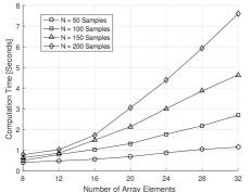
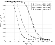
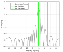
Figure 1: (a) CVX-based computation time of the Trace-Norm approach vs. number of elements ($P$) and number of samples ($N$). (b) The ratio between the first and second largest eigenvalues of $\hat{\mathbf{W}}$. (c) Averaged array pattern of the Trace-Norm solution, over 1000 experiments, with two CM signals: unit power from $20\degree$, and attenuated by random attenuation ($0dB$ to $-5dB$) from $60\degree$.

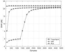
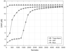
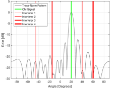
Figure 2: (a) SINR performance of the Trace-Norm, UKF and RLS ($p=1$, $\lambda=0.985$ , $\delta=0.001$) vs. number of samples (N), with noise variance $\sigma^{2}_{n}=0.1$, $P=16$ elements ULA, CM signal at $20\degree$; and three interferers at $-45\degree$,$-15\degree$ and $40\degree$; (b) with four interferers at $-45\degree$,$-15\degree$ , $40\degree$ and $60\degree$. (c) The resulting array pattern of the Trace-Norm solution, with 4 interferers, avergared over 1000 experiments.

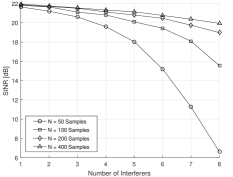
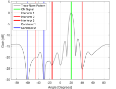
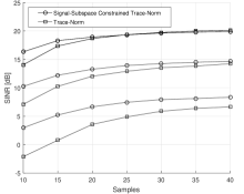
Figure 3: (a) SINR of the Trace-Norm solution vs. the number of interferers (SNR=10dB, P=16). (b) LCCMA Trace-Norm array pattern, with null constraints at $-30\degree$ and at $-60\degree$, and three interferers ($N=200$ samples, $\sigma^{2}_{n}=0.1$, $P=16$ elements). (c) SINR results of the Trace-Norm approach vs. the Signal-Subspace Constrained LCCMA Trace-Norm ($P=32$ elements) in the presence of a CM signal at $20\degree$, and 2 interferers at $-45\degree$,$-20\degree$: SNR = -5dB (lower curves); SNR = 0dB (middle curves); and SNR = 5dB (upper curves).

V Performance Evaluation

In this section we present computation time and simulation results illustrating the performance of our solution, referred to as Trace Norm. The performance is compared to the Recursive Least Squares (RLS) [8] and the Unscented Kalman Filter (UKF) [9] solutions.

The desired signal was simulated as a unit power QPSK signal. The interfering signals were simulated as complex Gaussian with zero mean and unit variance. The noise was simulated as a complex Gaussian with zero mean and covariance $\sigma^{2}_{n}\mathbf{I}$. The performance measure employed is the signal-to-interference-plus-noise ratio (SINR) at the beamformer output:

$$SINR=\frac{\mathbf{w}^{H}R_{ss}\mathbf{w}}{\mathbf{w}^{H}R_{nn}\mathbf{w}+\mathbf{w}^{H}R_{ii}\mathbf{w}},$$ (18)

where $R_{ss}=\mathbf{a}(\theta_{0})\mathbf{a}(\theta_{0})^{H}$, $R_{nn}=\sigma^{2}_{n}\mathbf{I}$, and $R_{ii}=\sum_{j=1}^{q}\mathbf{a}(\theta_{j})\mathbf{a}(\theta_{j})^{H}$are the CM signal, noise and interference covariance matrices, respectively. All presented results are averaged over 100 experiments, unless specified differently.

Experiment 1 evaluates the computation time of the Trace Norm solution. The worst case computational complexity of a general convex optimization problem is given by $O(\max(P,N)^{4}N^{0.5}\log(1/\epsilon))$ [17], where $\epsilon$ is the solution accuracy. To provide more typical results we evaluated the computation time using the MATLAB-based CVX [20] toolbox, and the results are presented in Fig. 1(a) Note that the speed-up factor between CVX-based implementation and a real-time implementation, as analyzed in [21], is in the range of $\times 100$ to $\times 10,000$ (single processor). The simulated scenario includes a CM signal impinging from $20\degree$ on a Uniform Linear Array (ULA) with $P=8$ to $P=32$ elements, and 3 interferers impinging from $-45\degree$ , $-15\degree$ and $40\degree$ (noise variance $\sigma^{2}_{n}=0.1)$.

Experiment 2 evaluates the ratio between the largest ($\lambda_{1}$) and the second largest ($\lambda_{2}$) eigenvalues of $\hat{\mathbf{W}}$, which is a good measure for the goodness of the rank-1 approximation of the trace norm solution of $\hat{\mathbf{W}}$. We evaluated this ratio by solving 500 times each of the following scenarios: a CM signal in the presence of 0,1, or 2 interferers, all signals are of equal power, at SNR of 10dB or 20dB ($\sigma^{2}_{n}=0.1$ or $0.01$, respectively). For the case of no interference, the ratio $\frac{\lambda_{1}}{\lambda_{2}}$ exceeded $10^{6}$ with probability 1, implying a perfect rank-1 result. Fig. 1(b) presents the results for the cases of 1 and 2 interferers, and reveals that $\frac{\lambda_{1}}{\lambda_{2}}\geq 10$, with probability 1, for SNR = 10dB, and$\frac{\lambda_{1}}{\lambda_{2}}\geq 50$ for SNR = 20dB. These results demonstrate the goodness of the rank-1 approximation of $\hat{\mathbf{W}}$.

Experiment 3 evaluates the performance of the Trace-Norm solution in the presence of two CM signals: The first from $20\degree$ with unit power, and the second from $50\degree$ ,attenuated in each trial by a random attenuation, uniformly distributed between 0dB to -5dB. Fig. 1(c) presents the averaged array pattern, over 500 experiments, and demonstrates the ”capture” effect of the Trace-Norm solution: the algorithm captures always the strongest CM signal, and cancels the weaker.

Experiment 4 compares the SINR of the Trace-Norm, UKF and RLS, in the presence of interferers. Note that since the Trace-Norm is a batch approach, whereas UKF and RLS are on-line approaches (processing one sample at time), the reported SINR, at each sample index $n$ , means that the algorithm processed all samples from the 1st until the $n$-th. In the first scenario we simulated a CM signal impinging from $20\degree$ on a 16 elements ULA, with 3 interfering signals impinging from $-45\degree$ , $-15\degree$ ,$40\degree$, and noise variance $\sigma^{2}_{n}=0.1$. The results are presented in Fig. 2(a) and demonstrate that the Trace-Norm solution obtain better SINR with only 100 samples, whereas UKF converges after $N=500$ samples, and RLS after $N=2,700$ samples. Fig. 2.(b). presents the performance with an additional interferer from 60°. In this case convergence of the UKF and RLS is slower ($N=1,500$ and $N=3,500$ samples, respectively), whereas the Trace-Norm is essentially invariant to to the addition of the interferer, and surpasses UKF and RLS with only 100 samples. The array pattern of the Trace Norm with $N=200$ samples (averaged over 1,000 experiments), is depicted in Fig. 2(c). The rejection of all 4 interferers is clearly visible.

Experiment 5 presents the SINR of the Trace-Norm solution vs. the number of interferers. The simulated scenario includes a CM signal impinging from $-25\degree$ on a 16 elements ULA, with a varying number of interferers between 1 to 8, impinging from directions chosen randomly from the following set of directions: $-85\degree,-70\degree,-55\degree,-40\degree,-10\degree,5\degree,20\degree,35\degree,50\degree,65\degree$ and $80\degree$. The noise variance per array element is $\sigma^{2}_{n}=0.1$, corresponding to SNR=10dB for all signals. The results presented in Fig. 3(a), demonstrate that the Trace-Norm solution can handle effectively (providing SINR>20dB) 3 interferers with $N=50$ samples, and 7 interferers with $N=400$ samples.

Experiment 6 demonstrates the ability of the Trace-Norm LCCMA to generate deep nulls in the array pattern in predefined directions, using the constraint (11),(12). The simulated scenario includes a CM signal at $20\degree$ impinging on a 16 element array, and 3 interferers from $-45\degree$,$-15\degree$ and $40\degree$ ($\sigma^{2}_{n}=0.1$). The nulls are constrained to directions $-30\degree$ and $-60\degree$. The resulting array pattern, averaged over 1,000 experiments, is depicted in Fig. 3(b). Clearly visible is the rejection of all interferers, as well as the deep nulls in the specified directions.

Experiment 7 demonstrates the performance advantage of the Trace Norm LCCMA over the Trace-Norm CMA when the constraint (11),(13) is imposed. The simulated scenario includes a CM signal impinging from $20\degree$ on a 32 elements ULA, with 2 interferers impinging from $-45\degree$ and $-20\degree.$ The SNR per array element is varied between -5dB to 5dB. The constraint (11),(13) forces the beamforming vector to be confined to the 3-dimensional signal subspace. Fig. 3(c) shows SINR results vs. the number of samples (N). The results demonstrate the advantage of the Trace Norm LCCMA over the Trace-Norm CMA for all signal-to-noise ratios (excluding a minor disadvantage for SNR=5dB and N>30 samples).

VI Conclusions

We have presented new convex-optimization-based solutions for the CMA and for the related problem of LCCMA. Our CMA solution was shown to provide much better performance than existing solutions based on UKF and RLS. Moreover, the SINR of our solution, was shown to approach the theoretical limit even for relatively small number of samples. We have also shown that our LCCMA solution enables the incorporation of a variety of linear constraints on the beamformer vector in a simple and effective way. We have shown that apart from enabling unity gain and null constraints to predefined directions, we can also incorporate more general constraints such as constraining the beamformer vector to the signal subspace. This was shown to provide significant performance gain as compared to unconstrained CMA.

References

- [1] D.N. Godard, Self-recovering equalization and carrier tracking in twodimensional data communication systems, IEEE Trans. Communications, vol. 28, pp. 1867 1875, Nov. 1980.
- [2] J. Triechler and B. G. Agee ”A new approach to multipath correction of constant modulus signals,” IEEE Trans. Acoust., Speech and Signal Process., vol. 31, pp. 459-472, Apr. 1983.
- [3] J. Treichler; M. Larimore ”New processing techniques based on the constant modulus adaptive algorithm,” IEEE Trans. Acous., Speech, and Signal Process., Vol. 33, pp. 420 - 431, 1985.
- [4] B.G. Agee ”The least squares CMA: A new technique for rapid correction of constant modulus signals,” In Proc. IEEE ICASSP, pp. 953-956, 1986.
- [5] R. Gooch and J. Lundell, The CM array: An adaptive beamformer for constant modulus signals, in Proc. IEEE ICASSP, pp. 2523-2526, 1986.
- [6] B. G Agee Blind separation and capture of communication signals using a multitarget constant modulus beamformer,” in Proc. MILCOM’89. 1989.
- [7] J. J. Shynk and R. P. Gooch, The constant modulus array for cochannel signal copy and direction finding, IEEE Trans. Signal Process., vol. 44, pp. 652-660, Mar. 1996.
- [8] Y. Chen, T. Le-Ngoc, B. Champagne, and C. Xu, ”Recursive least squares constant modulus algorithm for blind adaptive array,” IEEE Trans. Signal Process., vol. 52, pp. 1452-1456, May. 2004.
- [9] M. Z. A.. Bhotto, and I. V. Bajic, ”Constant Modulus Blind Adaptive Beamforming Based on Unscented Kalman Filtering”, IEEE Signal Process. Letters, vol. 22, Apr. 2015
- [10] A.J van der Veen and A. Leshem, ”Constant Modulus Beamforming,” in Robust beamforming. P. Stoica and J. Li eds. Wiley, 2005
- [11] M. J. Rude and L. J. Griffiths, ”A Linearly constrained Adaptive Algorithm for Constant Moudulus Signal Processing,” in Proc. EUSIPCO 92, Barcelona, pp. 237-240, 1992.
- [12] J. Miguez and L. CastedoL, ”A linearly constrained constant modulus approach to blind adaptive multiuser interference suppression,” IEEE Comm. Letters, vol. 2, pp. 217-219, Aug. 1998.
- [13] L. Wang and R.C. de Lamare ”Constrained Constant Modulus RLS-based Blind Adaptive Beamforming Algorithm for Smart Antennas,” in Proc IEEE ISWCS, pp. 657-661, 2007.
- [14] D. Liu and L. Tong. ”An analysis of constant modulus algorithm for array signal processing,” Signal Processing, vol. 73, pp. 81-104, 1999.
- [15] A. Leshem and A.J van der Veen, ”On the finite sample behaviour of the constant modulus cost function,” In Proc. IEEE ICASSP, pp. 2537-2540, 2000.
- [16] S. Boyd and L. Vandenberghe, Convex Optimization, Cambridge University Press, 2004.
- [17] Z.-Q. Luo; W.-K. Ma; A. M.-C So; Y. Ye and S. Zhang, ”Semidefinite Relaxation of Quadratic Optimization Problems,” IEEE Signal Process. Magazine, Vo. 27, pp. 20-84, 2010.
- [18] S. Ji and J. Ye, ”An Accelerated Gradient Method for Trace Norm Minimization,” Proc. of ICML, pp. 457-464, 2009.
- [19] K.-C Toh and S. Yun, ”An accelerated proximal gradient algorithm for nuclear norm regularized linear least squares problems,” Pacific Journal of optimization, 2010.
- [20] M. Grant and S. Boyd. CVX: Matlab software for disciplined convex programming, http://cvxr.com/cvx, September 2013.
- [21] J. Mattingley and S. Boyd, CVXGEN: a code generator for embedded convex optimization, Optim Eng, pp. 13-1 27, 2012.
- [22] H.L Van Trees, Optimum array processing, part IV of Detection, estimation, and modulation theory, Wiley, 2004.