An Ising Model for Metal-Organic Frameworks

Abstract

We present a three-dimensional Ising model where lines of equal spins are frozen in such that they form an ordered framework structure. The frame spins impose an external field on the rest of the spins (active spins). We demonstrate that this “porous Ising model” can be seen as a minimal model for condensation transitions of gas molecules in metal-organic frameworks. Using Monte Carlo simulation techniques, we compare the phase behavior of a porous Ising model with that of a particle-based model for the condensation of methane (CH₄) in the isoreticular metal-organic framework IRMOF-16. For both models, we find a line of first-order phase transitions that end in a critical point. We show that the critical behavior in both cases belongs to the 3D Ising universality class, in contrast to other phase transitions in confinement such as capillary condensation.

I Introduction

The Ising model has been a paradigm for the study of phase transitions. The analytical solution of the two-dimensional (2D) Ising model allowed for the first prediction of non-mean-field critical exponents onsager44 . Monte-Carlo simulations as well as renormalization group calculations of the three-dimensional (3D) Ising model have provided very accurate computations of critical exponents that establish the 3D Ising universality class ferrenberg91 ; pelissetto02 . Now, these exponents are known with very high precision thanks to the conformal bootstrap kos16 . Moreover, for phase transitions in confinement and in porous media, Ising models have provided a detailed understanding of wetting phenomena nakanishi82 ; ball88 ; ball89 ; binder03 as well as the exploration of novel condensation transitions such as interface localization-delocalization binder03 ; binder08 and the random-field Ising model universality class in disordered porous media (see, e.g., belanger91 and references therein).

Metal-organic frameworks (MOFs) are a relatively new class of porous media li99 ; eddaoudi02 ; yaghi03 ; rowsell05 , in which gases such as carbon dioxide (CO₂), water steam or methane (CH₄) can be stored via condensation on the framework structure rowsell05 ; rosi03 ; yildirim05 ; siberio07 ; uzun14 . MOFs form a crystalline porous network where metal-oxide centers are connected with each other by organic linkers. In this work, we consider the iso-reticular MOF structure IRMOF-16 in which the metal-oxide centers consist of an ordered arrangement of ZnO tetrahedra (see below). Gas condensation on various IRMOFs has been recently studied via Monte Carlo (MC) simulations in the grandcanonical ensemble mueller05 ; walton07 ; dubbeldam07 ; liu08 ; fairen10 ; toni10 ; hicks12 ; desgranges12 ; hoeft15 ; braun15 . These studies have found evidence for lines of first-order transitions that end in a critical point. In Refs. hoeft15 ; braun15 , it has been explicitly shown that for each of these condensation transitions there is coexistence of bulk phases that extend over the unit cells of the framework. Moreover, Höft and Horbach hoeft15 have demonstrated for the condensation of CH₄ in IRMOF-1 that there are two lines of first-order condensation transitions, both ending in a critical point. The first line at lower densities is associated with a novel type of phase transition on the surface of IRMOF-1 and has thus been denoted as IRMOF surface (IS) transition in Ref. hoeft15 . The second one, the IRMOF liquid-gas (ILG) line, can be seen as the analog of the liquid-gas line in bulk fluids.

Also the thermodynamic properties around the two critical points of CH₄ in IRMOF-1 were studied in Ref. hoeft15 . Evidence was given that the critical behavior belongs to the 3D Ising universality class. However, especially for the ILG critical point, the situation is not so clear. Here, the critical point is at a relatively high CH₄ density and thus the acceptance rates for insertion moves in the grand-canonical Monte Carlo simulation are low. This only allows to consider relatively small systems for which the corrections to finite-size scaling in terms of, e.g., the Binder cumulant binder81 are relatively large. To circumvent these problems, a minimal model of the Ising type would be helpful that shows a phase transition similar to the ILG transition for CH₄ in IRMOF-1. Then, one could more accurately investigate the critical behavior of the latter transition and rationalize that it is a member of the 3D Ising universality class.

In this paper, we propose a 3D Ising model where lines of equal spins are fixed. These lines are arranged such that they form a simple cubic framework structure. The fixed spins exert a field on the “mobile” active spins that tends to align the latter in the direction of the former. By compensating this field by a homogeneous external magnetic field acting on the active spins, coexistence may occur between a phase of positive and one of negative magnetization. In fact, via MC simulations we demonstrate the existence of a line of first order transitions that end in a critical point and compare the resulting phase diagram to MC simulations of the condensation of CH₄ in IRMOF-16. Different to our previous study hoeft15 , we consider IRMOF-16, because it has larger pores than IRMOF-1 and therefore the coexistence range of the ILG transition in IRMOF-16 is much broader than the one in IRMOF-1. Note that we do not find the IS transition line in IRMOF-16. Probably, these transitions occur at very low temperatures in IRMOF-16 and might be only metastable since the stable states are expected to be crystalline in this temperature range.

Both for the porous Ising model and CH₄ in IRMOF-16, in the MC simulations advanced sampling techniques are used, namely tethered and successive umbrella sampling fernandez09 ; virnau04 , respectively. At a given temperature $T$, these techniques allow to accurately determine the probability distributions $P({\cal O})$ of a variable ${\cal O}$ that is directly associated with the order parameter. Note that for the Ising model and the IRMOF-16 system the variables ${\cal O}$ are given by the magnetization, ${\cal O}=M$, and the density of the adsorbed gas, ${\cal O}=\rho$, respectively. Up to a constant $C$, the probability distribution $P({\cal O})$ corresponds to minus the logarithm of the free energy, $\beta F({\cal O})\propto-{\rm ln}P({\cal O})+C$ (with $\beta$ the inverse thermal energy), and therefore the full information about the thermodynamics of the system can be obtained from this quantity, in particular the phase diagram and quantities required for the finite-size scaling analysis around the critical point such as the Binder cumulant, the order parameter or the interfacial free energy. Our results indicate similar behavior of $P({\cal O})$ for the two considered systems. Compared to the corresponding bulk systems, in both cases the critical point shifts to lower temperature and a higher value of ${\cal O}$. While strong corrections to 3D-Ising behavior are seen for the IRMOF-16 system, as expected for the considered small system sizes in this case, for the porous Ising model our finite-size scaling analysis clearly indicates a critical behavior according to the 3D-Ising universality class.

The outline of the paper is as follows: In Sec. II, we introduce the models and the details of the simulations. Then, we present the results in Sec. II.3 and finally draw conclusions in Sec. II.4.

II Models and details of simulations and finite-size scaling analysis

II.1 Porous Ising model

In this section, the details of the porous Ising model are described. The layout of this section is as follows. In Sec. II.1.1, we introduce our Ising model. Given the spin/particle analogy that we aim to establish, we shall be mostly interested in the low temperature phases. These phases correspond to condensed phases in the particle system. The use of advanced sampling techniques is required at low temperatures that we introduce in Sec. II.1.2.

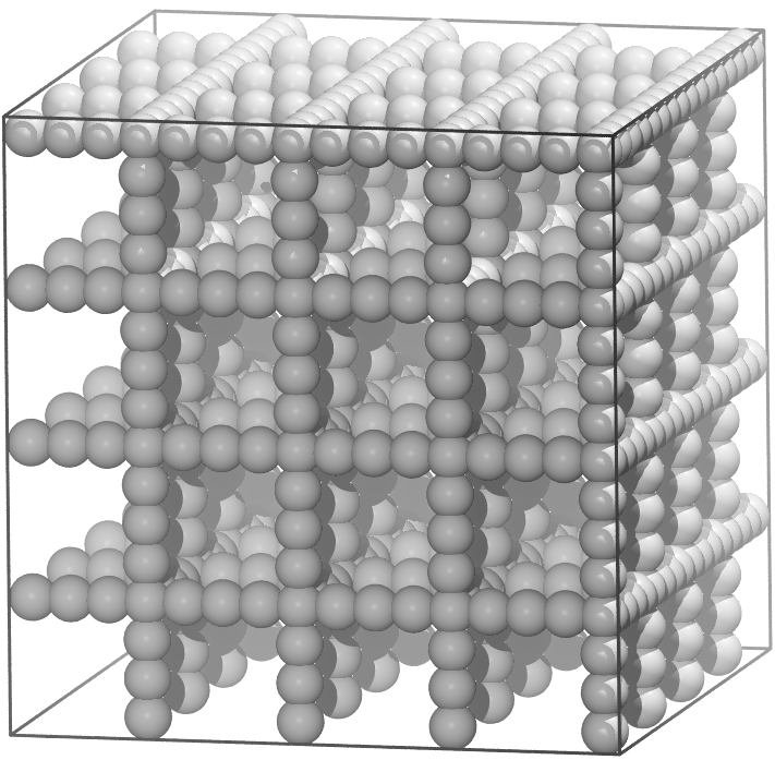
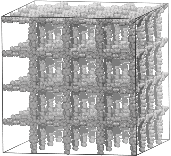
Figure 1: Porous networks of the Ising system showing the fixed spins only (upper panel) and IRMOF-16 (lower panel). A pore of the Ising model consists of 10 fixed spins, the IRMOF-16 framework pore contains 113 atoms.

II.1.1 Model

We consider $N$ Ising spins ($\sigma_{i}=\pm 1$) on a cubic lattice of size $L$, endowed with periodic boundary conditions. In this lattice, we shall distinguish two types of spins: the active ones and the frame spins.

The frame spins, depicted in the upper panel of Fig. 1, mimic the MOF, see the lower panel in Fig. 1. The frame is characterized by a period $P$ (we are assuming that $P$ divides exactly $L$). It is formed by straight lines parallel to the three lattice axis. We fix all the spins on the frame to $\sigma_{i}=1$.

The active spins are our dynamic variables. Their number is $\mathcal{N}_{\mathrm{act}}=N(P^{3}-3P+2)/P^{3}$, where $N=L^{3}$. The interaction energy of the system is given by the exchange term, introducing an interaction parameter $J>0$, and a coupling to an external magnetic field $h$

$${\cal H}=-J\sum_{\langle i,j\rangle}\sigma_{i}\sigma_{j}-h\sum_{i=1}^{N}\sigma_{j},$$ (1)

where $\sum_{\langle i,j\rangle}$ runs over all the couples of nearest neighbors. We consider all the spins, both frame and active ones, in Eq. (1). Therefore, at variance to the usual 3D Ising model (that we will refer as the bulk), the frame induces an effective positive magnetic field over the active spins even if $h=0$.

The order parameter of this system is linked to the magnetization of the active spins,

$${\cal M}=\sum_{i\in\mathcal{N}_{\mathrm{act}}}\sigma_{i}\,.$$ (2)

Note that one can interpret the Ising model as a lattice gas: $s_{i}=1$ (-1) meaning that a particle is present (absent) at site $i$. Therefore, the magnetization density relates to the particle-number density straightforwardly:

$$m={\cal M}/\mathcal{N}_{\mathrm{act}}=2\rho-1.$$ (3)

The presence of the fixed sublattice of spins displaces the phase diagram in the parameter space, as it is shown in Fig. 6 for the $P=4$ and $J=1$ model. However, the qualitative behavior of the phase diagram remains unaltered: a first order line that ends in a critical point separating a paramagnetic and ferromagnetic phases. The nature of this critical point could, in principle, change because of the symmetry break imposed by the sublattice. We will show that this point remains, being universal and in the 3D universality class.

In this work, we have considered three variants of this model: $J=1$ and $P=4$ (Model 1), $J=1$ and $P=8$ (Model 2), and $J=0.1$ and $P=4$ (Model 3). All the figures shown in this manuscript corresponds to Model 1. Results for the Models 2 and 3 are summarized in Table 1.

II.1.2 Simulation details for the porous Ising model

As we explained above, the magnetic/particle analogy made us focus on the low temperature phase. In that region, the system undergoes a first-order phase transition upon varying the applied field, $h$. Now, the simulation of first-order transitions is intrinsically difficult martin-mayor07 . This is why we shall refer to a special simulation method, named tethered Monte Carlo. Our description will be brief (the interested reader may consult Refs. fernandez09 ; martin-mayor11 ; fernandez12 ).

Tethered Monte Carlo is a sophistication of the traditional umbrella sampling torrie77 , where the constrained free-energy $W_{\beta}(\hat{m})$ is reconstructed by means of a (numerically exact) thermodynamic integration. The constrained free-energy is defined from

$$\mathrm{e}^{-NW_{\beta}(\hat{m})}=\sum_{\{\sigma_{i}\}}\mathrm{e}^{-\beta{\cal H}-\frac{1}{2}N(\hat{m}-m)^{2}}\,.$$ (4)

In the above expression, the sum runs over all possible configurations of the active spins, while $\beta$ stands for the inverse temperature $1/T$. It is clear from the definition that $W_{\beta}(\hat{m})$ is the constrained free energy needed to keep the system at a magnetization $m(={\cal M}/N_{\mathrm{act}})\approx\hat{m}$ at temperature $T$ and at zero external magnetic field.

From $W_{\beta}(\hat{m})$, one can trivially recover the canonical partition function in a magnetic field as

$$\int{\rm d}\hat{m}\;\mathrm{e}^{-NW_{\beta}(\hat{m})+N\beta h\hat{m}}=Z(h,T)\,\mathrm{e}^{\frac{1}{2}N\beta^{2}h^{2}}\,.$$ (5)

It follows that the tethered parameter $\hat{m}$ and the magnetization density are related as:

$$\langle\hat{m}\rangle_{\beta,h}=\langle m\rangle_{\beta,h}+\beta h\,.$$ (6)

What one actually computes in a tethered computation is the derivative with respect to $\hat{m}$

$$W_{\beta}^{\prime}(\hat{m})=\langle\hat{m}-m\rangle_{\hat{m},\beta}\,.$$ (7)

Therefore, we numerically compute $W_{\beta}^{\prime}(\hat{m}_{i})$ on a grid $(\hat{m}_{i},T)$, with $i=1,\ldots N_{m}$. The entire potential can later be recovered by means of a numerical integration of these points. From this, we determine very precisely the location of the first-order transition at a given temperature $T$, that is, the coexistence field $h_{\mathrm{co}}$ and the position of the positive $\hat{m}^{+}$ and negative $\hat{m}^{-}$ magnetization minima of the total free-energy potential. This amounts to performing a Maxwell construction martin-mayor07 :

$$\log\frac{p_{\beta,h}(\hat{m}^{+})}{p_{\beta,h}(\hat{m}^{-})}=-N\int_{\hat{m}_{-}}^{\hat{m}^{+}}\left(W_{\beta}^{\prime}(\hat{m})-h_{\mathrm{co}}\right){\rm d}\hat{m}=0.$$ (8)

$W_{\beta}^{\prime}(\hat{m})-h_{\mathrm{co}}$ has at least three roots: the magnetization of the two pure phases $\hat{m}^{-}$, $\hat{m}^{+}$, and a central point magnetization, $\hat{m}^{*}$, that corresponds to a half-half configuration of the two ferromagnetic phases. We can use this fact to obtain the free-energy cost to build the two interfaces (because of the periodic boundary conditions) of size $L^{2}$, by comparing the free-energy of the mixed configuration with $\hat{m}=\hat{m}^{*}$, and of the pure phase. Once the cost in free-energy is known, the surface tension follows:

$$\Sigma_{\beta}=\frac{N}{2L^{2}}\int_{\hat{m}^{-}}^{\hat{m}^{*}}\left(W_{\beta}^{\prime}(\hat{m})-h_{\mathrm{co}}\right){\rm d}\hat{m}.$$ (9)

Alternatively, one can also obtain the first-order transition line, as well as to expand it into the paramagnetic phase (which is known as the Widom line widom65 ), by looking for the value of $h$ that makes $p_{\beta}(\hat{m};h)$ symmetrical, in practice, by extracting the value of $h$ at which the skewness of the probability distribution vanishes parisi14 . This approach allows us to compute the Binder cumulant binder81 , $U_{L}$, for a given linear dimension $L$ of the simulation box as the kurtosis of the distribution along this line,

$$U_{L}(T,h)=1-\frac{1}{3}\frac{\langle\,(\hat{m}-\langle\hat{m}\rangle_{\beta,h})^{4}\,\rangle}{\langle\,(\hat{m}-\langle\hat{m}\rangle_{\beta,h})^{2}\,\rangle^{2}}\,.$$ (10)

Before we go on a word of caution is in order. Dimensionless quantities such as $U_{L}$ or the surface tension $L^{2}\Sigma_{\beta}$, are expected to enjoy only a restricted degree of universality at the critical point. Their value is expected to be independent of any microscopic details of the interactions, however they are sensitive to several geometric features. For instance, changing boundary conditions or the lattice geometry (say, going from a cubic to an elongated box) must result in a variation of their value. The question arose in the original paper by Binder binder81 , and has been throughly studied numerically in bulk systems selke06 ; selke07 ; selke09 . The reason for this geometric sensitivity is particularly clear for the Binder cumulant $U_{L}$, which can be computed from space integrals of universal scaling functions salas00 . The scaling functions themselves are insensitive to microscopic details such as the interaction range, etc. Yet, the value of the integrals that yield $U_{L}$ are sensitive to the geometry of the integration domain.

We have performed two sets of simulations, a coarse one to determine the position of the first-order transition branches and to get a rough idea of the position of the critical point, and an extensive study of the critical point. For the first part of the study, we used a mesh of $m$ points with a width of $\delta m=0.1$, while for the second part, we reduced this width to $\delta m=0.003$. For determining the first-order transition lines, we performed simulations at different temperatures and $N=16,\ 32$ and $64$, while for the critical point we just simulated one temperature for each model $T_{\mathrm{sim}}\sim T_{\mathrm{c}}$, $T_{\mathrm{sim}}$ is shown in Table 1, and extrapolated results to nearby temperatures using the re-weighting method ferrenberg88 . In order to compute the critical point and its critical exponents shown in Table 1, we used the quotients method amit05 ; ballesteros00 , for which we studied the crosses of the curves of $\Sigma L^{2}$ and $\Delta m=\hat{m}^{+}-\hat{m}^{-}$ between curves coming from systems at system sizes $L$ and $2L$. With this scheme, we studied $L=8,\ 12,\ 16,\ 24,\ 32,\ 48$ and $64$.

A difficulty we encounter in the present setting is that the phase diagram is two-dimensional $(T,h)$. We shall eliminate one variable by fixing the magnetic field to its coexistence value $h_{\mathrm{co}}(T)$, see Eq. (8).

II.2 CH₄ in IRMOF-16: Model and simulation details

IRMOF-16 is modeled as a rigid framework, consisting of carbon (C), hydrogen (H), zinc (Zn), and oxygen (O) atoms. The information about the relative positions of these atoms are taken from X-ray diffraction data li99 (see Figs. 1b and 2). CH₄ molecules are described as Lennard-Jones (LJ) point particles, as proposed by Martin and Siepmann martin98 . Also the interactions of the CH₄ particles with the framework atoms are modeled by LJ potentials, employing the universal force field (UFF) of Rappé et al. rappe92 . Details on the interactions parameters can be found in Ref. hoeft15 .

The MC simulations for the particle-based model of CH₄ in IRMOF-16 are performed in the grand-canonical ensemble, i.e. at constant volume $V$, temperature $T$, and chemical potential $\mu$. The chemical potential is the analog of the external magnetic field $h$ in the porous Ising model. While the field $h$ is the thermodynamic conjugate variable of the total magnetization ${\cal M}$, the chemical potential $\mu$ is thermodynamically conjugate to the number of CH₄ particles $N$. Thus, by changing the intensive variables $h$ in case of the Ising model and $\mu$ in case of the CH₄ in IRMOF-16, the average magnetization ${\cal M}$ and the average particle number $N$, respectively, can be varied; in particular, at a given temperature below the critical temperature $T_{c}$, the intensive variables $h$ and $\mu$ can be tuned such that coexistence conditions are obtained. To this end, histogram reweighting is also used for the particle-based model, as describe above for the Ising model. Similarly to the tethered MC, used for the Ising model, the MC for the IRMOF system is combined with successive umbrella sampling virnau04 which allows for an accurate estimate of the probability distribution $P(\rho)$ in the two-phase region (with $\rho$ the number density of CH₄ particles, $\rho=N/V$). Details on the implementation of the grand-canonical MC in combination with successive umbrella sampling for MOFs are given in a previous publication hoeft15 .

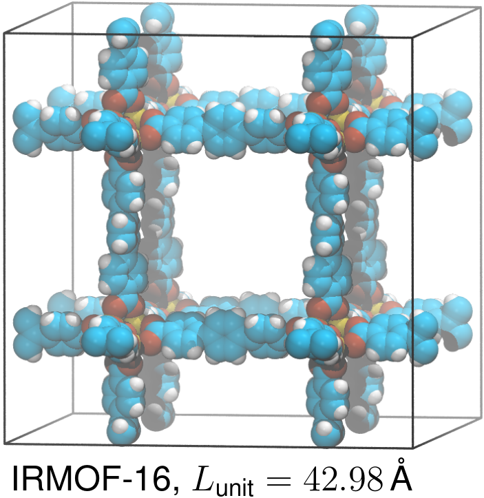
Figure 2: Unit cell of IRMOF-16. The length $L_{\rm unit}=42.980$ Å corresponds to the linear dimension of the unit cell. Atoms are shown as spheres with different colors, namely C (turquoise), H (white), O (red), and Zn (yellow).

Simulations for different system sizes in a cubic box geometry are performed. The considered linear dimensions of the boxes are $L_{\rm MOF}=1.0$ $L_{\rm unit}$, $1.5$ $L_{\rm unit}$, and $2.0$ $L_{\rm unit}$, with $L_{\rm unit}=42.980$ Å the size of the unit cell (see Fig. 2). Low acceptance probabilities of the order of $10^{-3}$ for trial insertions of CH₄ particles did not allow the simulation of larger system sizes. To improve the statistics, for all the systems 10 independent runs were done at each temperature.

II.3 Results

The central quantity, obtained from the MC simulations for the two models, is the order parameter distribution function $P({\cal O})$. Under coexistence conditions of a first-order phase transition, this function becomes bimodal such that two peaks, located at ${\cal O}^{(1)}$ and ${\cal O}^{(2)}$ and with equal area under both peaks, occur binder84 ; borgs90 . To obtain the coexistence field $h$ in case of the porous Ising model and the coexistence chemical potential in case of the IRMOF system, we employ histogram reweighting techniques ferrenberg88 .

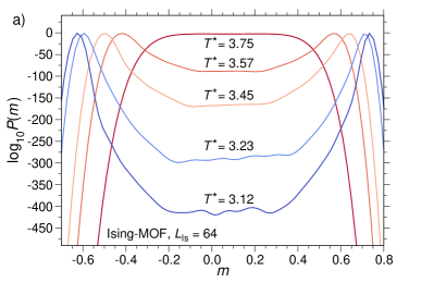
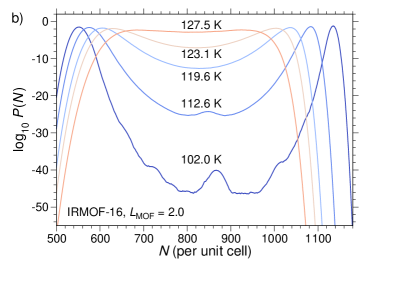
Figure 3: Probability distributions for a) Ising-MOF model and b) in IRMOF-16 model as determined from the largest available systems, as indicated by the edge lengths of cubic system sizes, $L_{\rm Is}$ and $L_{\rm MOF}$.

Figure 3 displays the logarithm of coexistence probability distributions for the lattice model and the particle-based systems at different temperatures below the critical temperature. Note that the figures show data for the largest systems, simulated in the respective cases. For the Ising model, two peaks can be seen at each temperature and the distance between the peak maxima decreases as approaching the critical temperature. Between the peaks, there is a plateau region, developing ripples for low temperatures, $T\lesssim 3.23k_{B}J$. The plateau in $P(m)$ corresponds to the two-phase region where the coexisting phases with magnetization $m^{+}$ and $m^{-}$ are separated from each other by a planar interface (cf. the snapshot, Fig. 5a). The distance between the height of the peaks and the height of the plateau are proportional to the surface tension, $\Sigma$, required for the formation of an interface. The ripples indicate a dependence of $\Sigma$ on $m$ in the two-phase region. We will clarify the source of this behavior below.

For comparison, the probability distribution $P(N)$ of the ILG transition of CH₄ in IRMOF-16 (Fig. 3b) shows a similar behavior as the corresponding function for the Ising model. However, one has to keep in mind that the considered system size for the atomistic model is much smaller the one for the Ising model. While the IRMOF-16 system consists of $2^{3}$ unit cells or 64 pores, systems with $64^{3}$ pores are simulated in case of the Ising model. As we can infer from the distributions in Fig. 3b, the oscillations in the regions between the two peaks are much more pronounced for the IRMOF-16 system and, as we shall see now, this is due to the much smaller system size considered in this case.

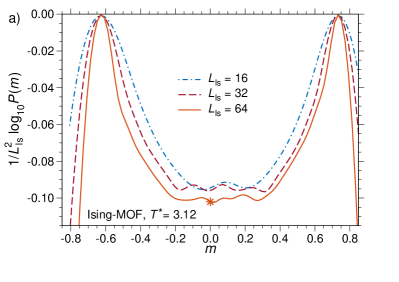
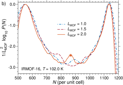
Figure 4: Semilogarithmic plots of the probability distributions for different system sizes scaled with the area of the planar interface, $1/L_{\rm Is}^{2}$ and $1/L_{\rm MOF}^{2}$ for a) the Ising model and b) the IRMOF-16 system, respectively. Red stars in a) and b) refer to the corresponding snapshots in Fig. 5.

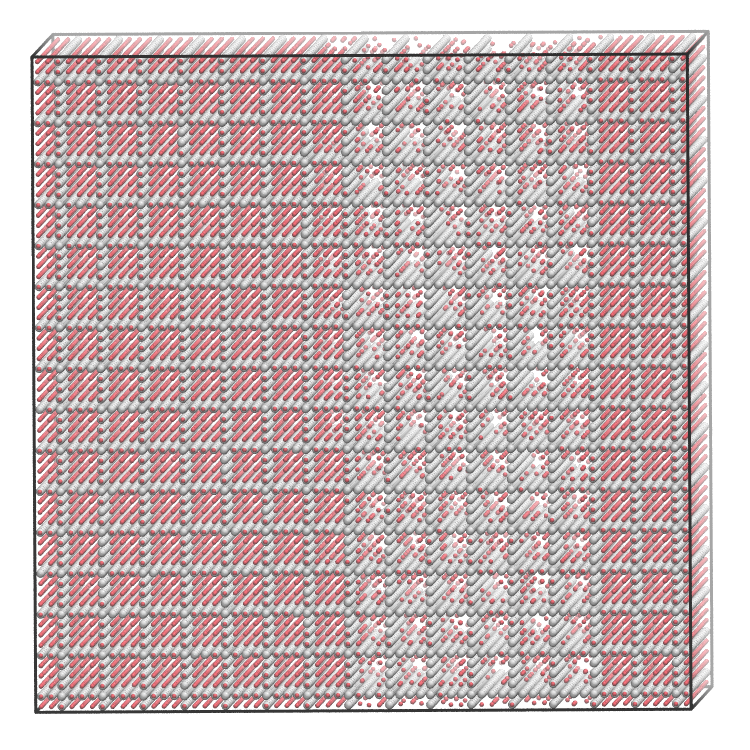
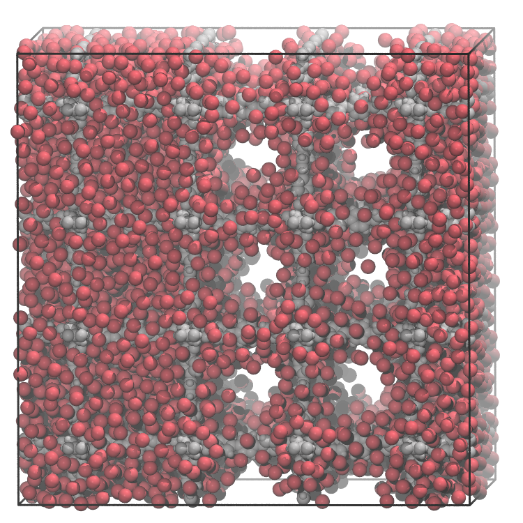
Figure 5: Configuration snapshots at coexistence conditions for the Ising-MOF model at $T=3.12k_{B}/J$ (upper panel), no magnetization ($m=0$) showing spins with $\sigma=1$ only (active spins in red, fixed framework spins in gray); and the IRMOF-16 model, at $T=102$ K with $N=864$ per unit cell (lower panel). Red and gray spheres represent CH₄ molecules and framework atoms, respectively.

To this end, we scale the logarithm of the probability distributions by the area of the interface, $L_{\rm Is}^{2}$ and $L_{\rm MOF}^{2}$ for the Ising model and the atomistic MOF system, respectively. In Fig. 4, scaled distributions for different system sizes are plotted, for both the lattice model and the atomistic system at a temperature far below the critical temperature, corresponding to the lowest temperatures shown in Fig. 3. As one can infer from $P(m)$ in Fig. 4a, with increasing system size, the width of the two peaks decreases while the flat region between the two peaks becomes broader. Moreover, the distance between maxima and the minimum in $P(m)$ is slightly increasing with increasing system size. This is due to the fact that in the smaller system the two interfaces are not sufficiently separated from each other and thus the interaction between the two interfaces leads to an effective decrease of the free energy cost of the interfaces. Also the oscillations in the plateau region of $P(m)$ are less pronounced for the large system. That these oscillations are expected to vanish in the thermodynamic limit can be understood as follows: In the two-phase region, the lever rule controls the amount of the two coexisting phases with magnetizations $m^{+}$ and $m^{-}$. Under this constraint, in a finite system only for certain values of $m$, flat interfaces can be embedded into the framework structure such that its free energy cost is minimized. This happens when the flat interface is located in a plane that goes through the corners of the framework structure (cf. the snapshot for the system with $L_{\rm Is}$, Fig. 5a, corresponding to a minimum in the plateau region of $P(m)$, marked by the star in Fig. 4a). In the thermodynamic limit, a flat interface can be always arranged according to a minimal free energy cost and thus the oscillations tend to disappear for sufficiently large system sizes. This is also the case if the width of the interfacial region is of the order of the linear dimension of the unit cell of the framework, as is expected at sufficiently high temperatures, i.e. close enough to the critical temperature. Indeed, as Fig. 4 indicates for the largest system, this happens for temperatures that are about 10-20% below the critical temperature which is around 3.75 (see below).

The scaled distributions for the IRMOF-16 system (Fig. 4b) exhibit a similar behavior. However, due to the small system sizes, finite-size effects are much more pronounced. As one can infer from the snapshot (Fig. 5b), even for the IRMOF-16 system with $L_{\rm MOF}=2.0$ the distance between the two interfaces is less than the linear dimension of the unit cell. Therefore, $\log P(N)$ shows very pronounced oscillations in the two-phase region.

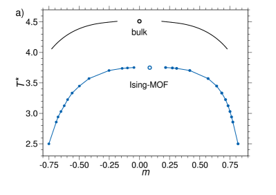
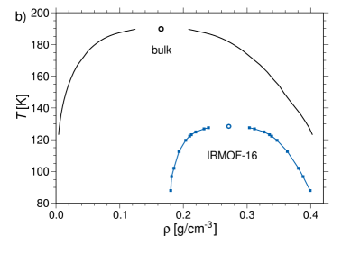
Figure 6: Phase diagram showing binodal lines of a) the Ising system and b) CH₄ in IRMOF-16, showing the ILG phase transition, each in comparison to the bulk binodal. Critical points are shown as open symbols.

The phase diagrams in the magnetization-temperature and the density-temperature plane for the porous Ising model and CH₄-IRMOF-16, respectively, are shown in Fig. 6. Here, the coexistence magnetizations and densities were directly determined from the first moments of each of the peaks in $P(m)$ and $P(N)$, respectively. Also included in the figure are the phase diagrams for the corresponding bulk systems. Compared to the bulk, in both porous systems the critical temperature $T_{c}$ is significantly lower. An analogous effect is also known from capillary condensation in thin films fisher81 and, similarly as in thin films, it is due to the attraction of gas molecules by the framework structure for the atomistic system and the alignment of the active spins with the framework spins in case of the porous Ising model. Note that the critical temperature of the Ising system could potentially be tuned to match the behavior of bulk methane compared to methane in IRMOF-16. This could be accomplished by varying the interaction strength of the active spins with the framework spins.

The two-phase region is narrower in the presence of the framework structure which is also similar to systems in thin films confinements. However, in thin films, a crossover from 3D to 2D-Ising scaling behavior close to the critical point is observed nakanishi82 . Such a cross-over is absent in our case, as we demonstrate now by a detailed finite-size scaling analysis.

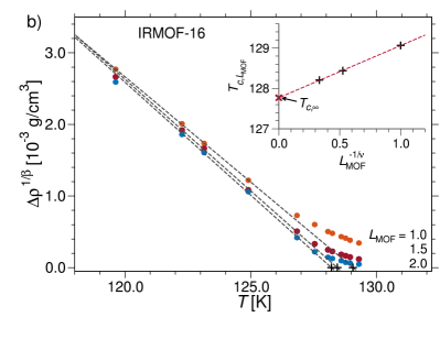
Figure 7: Rectification plot of the order parameter ${\cal O}$ for a) the Ising model (with ${\cal O}=\Delta m$) and b) the IRMOF-16 system (with ${\cal O}=\Delta\rho$). The insets show $T_{c}^{L_{\rm Is}}$ and $T_{c}^{L_{\rm MOF}}$ as a function of $L_{\rm Is}$ and $L_{\rm MOF}$, respectively. For the exponents, the 3D Ising values $\beta=0.326$ and $\nu=0.63$ hasenbusch10 are used.

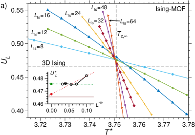
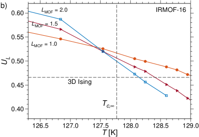
Figure 8: a) Binder’s cumulant $U_{L}$ for the Ising-MOF system for different system sizes $L$ close to the critical temperature. The inset shows the intersection value of $U_{L}$, $U_{L}^{\text{*}}$, as a function of system size and fits extrapolating $U_{L}^{\text{*}}$ to $L\to\infty$ using a linear function (red) and a constant (green). The figure in b) shows the same cumulant for IRMOF-16. 3D Ising universal values of $U_{L}^{\text{*}}\approx 0.465$ are included as indicated.

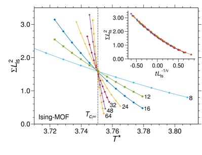
Figure 9: Surface tension, $\Sigma$ multiplied by $L_{\rm Is}^{2}$ for all system sizes, as indicated by the numbers for $L_{\rm Is}$. In the main panel $\Sigma L_{\rm Is}^{2}$ is shown as function of temperature $T^{*}$ and in the inset as function of the scaling variable $tL^{1/\nu}$ with $t=\frac{T-T_{c}}{T_{c}}$ using the 3D Ising universal value $\nu=0.63$.

An appropriate order parameter ${\cal O}$ for the porous Ising model is the difference between the magnetizations of the coexisting ferromagnetic phases (${\cal O}=\Delta m$). A similar order parameter for the IRMOF-16 system is the density difference between the coexisting CH₄ fluids (${\cal O}=\Delta\rho$). Approaching the critical point from below along the binodal, the order parameter is expected to vanish as

$${\cal O}\propto\left(T_{c,L}-T\right)^{\beta},$$ (11)

provided that the temperature difference $T_{c,L}-T$ is sufficiently small. Here, $T_{c,L}$ is the critical temperature corresponding to a cubic system with linear dimension $L$. In the following, $T_{c,L_{\rm Is}}$ and $T_{c,L_{\rm MOF}}$ denote the finite-size critical temperatures for the Ising and the IRMOF-16 model, respectively. Using the appropriate exponent $\beta$ in Eq. (11), one would obtain a straight line in a plot of ${\cal O}^{1/\beta}$ vs. $T$ that intersects the $x$-axis at $T_{c,L}$. The critical temperature in the thermodynamic limit, $T_{c,\infty}$, can be determined via ferrenberg91

$$T_{c,L}=T_{c,\infty}+AL^{-1/\nu},$$ (12)

with $A$ a critical amplitude and $\nu$ the critical exponent that describes the divergence of the correlation length. Figure 8 shows the rectification plots for the order parameter using the value $\beta=0.326$ hasenbusch10 , predicted for the 3D-Ising universality class. As insets, the scaling plots for the critical temperatures according to Eq. (12) are displayed. Here, the 3D-Ising value $\nu=0.63$ is used hasenbusch10 . The scaling works nicely for the Ising model, resulting in the estimate $T_{c,\infty}=3.7507$. The rectification plots for the IRMOF-16 system indicate strong deviations from a straight line for small values of $(\Delta\rho)^{1/\beta}$. This is very likely due to higher-order corrections to the finite-size scaling prediction, Eq. (11), see also Ref. ferrenberg91 . For the atomistic system, the estimate for the critical temperature in the thermodynamic limit is $T_{c,\infty}=127.8$ K. The critical temperature can be also obtained from the Binder cumulant $U_{L}$ binder81 . For the Ising model, $U_{L}$ is defined by Eq. (10). In Fig. 8a, the cumulant $U_{L}$ for the Ising model is plotted as a function of temperature for different values of $L$. In the finite-size scaling regime of the isotropic 3D bulk Ising model, $U_{L}$ for different $L$ is expected to intersect at the critical temperature and a universal value $U_{L}^{*}=0.61069$ for the 2D Ising kamienarz93 and $U_{L}^{*}=0.4655$ for the 3D Ising universality class luijten02 . From Fig. 7a small corrections to finite-size scaling can be inferred. However, we can extrapolate $U_{L}^{\text{*}}$ to the thermodynamic limit $L\to\infty$. Plotting $U_{L_{i}}^{\text{*}}$, as a function of $L^{-\omega}$ and extrapolating this using a linear approximation via $U_{L}^{\text{*}}(x=L^{-\omega})=mx+c$ by fitting the parameters $m$ and $c$. Such extrapolation can be found in the inset of Fig. 8a, also including an extrapolation using a constant, as it appears to work equally well. In both cases we observe a deviation to $U_{L}^{\text{*}}$ as obtained by hasenbusch10 for the 3D Ising universality class, which allows us to conclude the external framework potential introduces (small) corrections to $U_{L}^{\text{*}}$ compared to the bulk system. For the IRMOF-16 system, the Binder cumulant is defined by $U_{L}=1-\frac{\langle\rho^{4}\rangle}{3\langle\rho^{2}\rangle^{2}}$, with $\langle\rho^{2}\rangle$ and $\langle\rho^{4}\rangle$ being respectively the second and fourth order moments of the probability distribution $P(\rho)$, $\langle\rho^{n}\rangle=\int d\rho\rho^{n}P(\rho)$ with $n=2$ and $n=4$, respectively. As Fig. 7b indicates, due to the small system sizes the corrections to the finite-size scaling regime are much stronger for the CH₄-IRMOF-16 system. Nevertheless, one can conclude also in this case that the behavior of the cumulants is at least consistent with 3D-Ising universality (however, the MOF geometry might change its value, as we discussed below Eq. (10)).

Finally, we present a more refined finite-size scaling analysis for the Ising-MOF system, from which our most accurate results follow (the so-called quotients method, see Refs. nightingale76 ; ballesteros96 ; amit05 ). Unfortunately, the atomistic MOF systems that we can simulate are far too small to reproduce this analysis.

The starting point is identifying a dimensionless scaling function. In our case, the easiest to compute (and also the most accurate one) is the free-energy cost of introducing a system-wide interface, namely $\Sigma L^{2}$, see Eq. (9). Finite-size scaling tells us that $\Sigma L^{2}$ scales as

$$\Sigma L^{2}=g\Big{(}L^{1/\nu}(T-T_{\mathrm{c}})\Big{)}+{\cal O}(L^{-\omega})\,,$$ (13)

where $g$ is a smooth scaling function and $\omega$ is the universal leading corrections to scaling exponent. Therefore, barring scaling corrections, if we plot $\Sigma L^{2}$ as a function of $T$ for several system sizes as we do in Fig. 9, the curves will cross at $T_{\mathrm{c}}$. Alternatively, if we represent $\Sigma L^{2}$ as a function of $L^{1/\nu}(T-T_{\mathrm{c}})$ data from different system sizes should collapse onto a master curve, see the inset of Fig. 9.

In order to perform a precision computation of $T_{\mathrm{c}}$ and the critical exponents, we consider pairs of lattices of sizes $(L_{1},L_{2})$. We shall fix their ratio $s=L_{2}/L_{1}$ and consider the limit of large $L=L_{1}$. The corresponding curves $\Sigma L_{1}^{2}$ and $\Sigma L_{2}^{2}$, see Fig. 9, cross at a temperature scaling as

$$T^{(L,sL)}=T_{\mathrm{c}}+A\frac{1-s^{-\omega}}{s^{1/\nu}-1}L^{-(\omega+\frac{1}{\nu})}\,,$$ (14)

where $A$ is an amplitude and we have considered only the leading corrections to scaling binder81 . We have mostly considered $s=2$ for the ratio of system sizes. This equation is used to obtain another independent estimate of the critical temperature.

As for the critical exponents, let us consider a generic quantity $O$ that, in the $L=\infty$ limit, diverges as $\langle O\rangle\sim 1/|T-T_{\mathrm{c}}|^{x_{O}}$. Finite size scaling implies that $\langle O\rangle_{L}=L^{x_{O}/\nu}g_{O}(L^{1/\nu}(T-T_{\mathrm{c}})$, where $g_{O}$ is an unknown but smooth scaling function. Then it is easy to see that the ratio evaluated at the crossing point $T^{(L,sL)}$ scales as

$$\frac{\langle O\rangle_{sL}(T^{(L,sL)})}{\langle O\rangle_{L}(T^{(L,sL)})}=s^{x_{O}/\nu}+A_{O}L^{-\omega}\,.$$ (15)

In the above expression, $A_{O}$ is an amplitude, and we have kept only the leading corrections to scaling.

	bulk hasenbusch10	Model 1	Model 2	Model 3
$\beta_{\mathrm{sim}}$		0.2666	0.2339	0.2564
$\beta_{\mathrm{c}}$	0.22165463(8)	0.266642(7)	0.233961(6)	0.256359(5)
$h_{\mathrm{c}}$	0	-0.563515(2)	-0.114187(5)	-0.0566572(7)
$\nu$	0.63002(10)	0.629(9)	0.629(5)	0.628(5)
$\eta$	0.03627(10)	0.027(14)	0.03(3)	0.04(7)
$(\Sigma L^{2})^{*}$	$-$	1.57(3)	1.58(8)	1.600(19)

Table 1: Extrapolation of the critical points and exponents to the thermodynamical limit for the three models studied. These results are obtained with tethered MC simulations containing at least $N_{m}=184$ points at $\beta_{\mathrm{sim}}\sim\beta_{\mathrm{c}}$, and using the reweighting method ferrenberg88 to extrapolate to nearby values of $\beta$. The exponents are extracted using the quotients method, see Eq. (15). For the bulk universality class, we should also recall the most precise known results $\nu=0.629971(4)$ and $\eta=0.036298(2)$ that were obtained with the conformal bootstrap kos16 (this technique cannot provide $\beta_{\mathrm{c}}$).

We employ Eq. (15) with the derivative $\partial_{T}\Sigma$ ($x_{\partial_{T}\Sigma}=1-2\nu$), and with $(\Delta m)^{2}$, see Fig. 7a ($x_{(\Delta m)^{2}}=2-\eta$ ($\eta$ is the anomalous dimension, see e.g. amit05 ). The results of this analysis are summarized in Table 1. In the table we present results for the main model studied here and include as well exponents for two modified versions of the Ising-MOF model, one with doubled periodicity $P$ and with decreased spin-spin coupling constant $J$. As expected, in both cases the phase behavior becomes more bulk-like with respect to the critical temperature shift and the external field at the critical point, $h_{c}$.

II.4 Conclusions

In this work, an Ising model for the adsorption of gas molecules in metal-organic frameworks (MOFs) has been presented. The phase behavior of this model has been directly compared to an atomistic simulation of methane (CH₄) in IRMOF-16. The MOF-Ising model consists of frozen lines of equal spins that are arranged such that they form an ordered network with a cubic framework structure. Although the pores of the proposed Ising model are extremely narrow (note that in our model 1 the lines of frozen spins appear with a periodicity $P=4$), it exhibits a line of first-order order transitions, each with the coexistence of bulk phases, i.e. ferromagnetic phases, that extend over the unit cells of the framework structure. A qualitatively similar phase behavior is found for the atomistic MOF system and thus the MOF-Ising model can be considered as a minimal model for the adsorption of gas molecules in MOFs.

The line of first-order transitions both in the MOF-Ising model and the atomistic CH₄-IRMOF-16 system ends in a critical point. Consistent with the observation of first-order transitions with coexisting three-dimensional bulk phases, one may conjecture that the critical behavior of the MOF systems belongs to the 3D Ising universality class. However, this would imply that there is a divergent correlation length that grows over the unit cells of the framework structure when approaching the critical point. The existence of such a critical behavior has hardly any counterpart in other systems with 3D Ising universality. So it is a non-trivial issue whether the conjecture of 3D Ising behavior associated with the adsorption transitions in MOFs holds. For the atomistic MOF system, the accessible system sizes are too small to convincingly confirm the latter conjecture. However, for the MOF-Ising system we have rationalized in this work that the critical behavior is consistent with 3D Ising behavior. To this end, we have performed a detailed finite-size scaling analysis of the order parameter, the Binder cumulant and the surface tension.

The proposed MOF-Ising model can be easily extended to describe also other phenomena, associated with the gas adsorption in MOFs. The IS transition, where the coexisting phases form on the surface of the framework structure, can be realized by an inhomogeneous distribution of the interaction parameter $J$ describing the interaction between a frozen and an active spin. Frozen up-spins sitting in the corners of the framework structure (“metallic centers”) shall have stronger attractive interactions with the active spins than the rest of the framework up-spins on the “linkers”. In this manner, one could stabilize a phase with an enrichment of active up-spins at the corners of the framework and thus there is the possibility of a phase transition from the latter phase to one where there is an enrichment of active up-spins around the surface of the whole framework. Another interesting theme would be the investigation of phase-ordering kinetics in MOF-Ising models. Due to the framework of frozen spins, the domain coarsening in MOF systems is expected to be very different from that in typical bulk fluids. The MOF-Ising model is very well suited for the study of phase-ordering kinetics since it allows to consider relatively large length and time scales and, as a consequence, the scaling behavior and the morphology of the coarsening dynamics could be investigated in detail. All these issues shall be addressed in forthcoming studies.

- (1) L. Onsager, Phys. Rev. 65, 117 (1944).
- (2) A. M. Ferrenberg and D. P. Landau, Phys. Rev. B 44, 5081 (1991).
- (3) A. Pelissetto and E. Vicari, Phys. Rep. 368, 549 (2002).
- (4) F. Kos, D. Poland, D. Simmons-Duffin, and A. Vichi, Journal of High Energy Physics 08, 36 (2016).
- (5) H. Nakanishi and M. E. Fisher, Phys. Rev. Lett. 49, 1565 (1982).
- (6) P. C. Ball and R. Evans, J. Chem. Phys. 89, 4412 (1998).
- (7) P. C. Ball and R. Evans, Langmuir 5, 714 (1989).
- (8) K. Binder, D. Landau, and M. Müller, J. Stat. Phys. 110, 1411 (2003).
- (9) K. Binder, J. Horbach, R. Vink, and A. De Virgiliis, Soft Matter 4, 1555 (2008).
- (10) D. P. Belanger and A. P. Young, J. Magn. Magn. Mater. 100, 272 (1991).
- (11) H. Li, M. Eddaoudi, M. O’Keeffe, and O. M. Yaghi, Nature 402, 276 (1999).
- (12) M. Eddaoudi, J. Kim, N. Rosi, D. Vodak, J. Wachter, M. O’Keeffe, and O. M. Yaghi, Science 295, 469 (2002).
- (13) O. M. Yaghi, M. O’Keeffe, N. W. Ockwig, H. K. Chae, and M. Eddaoudi, Nature 423, 705 (2003).
- (14) J. L. C. Rowsell, E. C. Spencer, J. Eckert, J. A. K. Howard, and O. M. Yaghi, Science 309, 1350 (2005).
- (15) N. L. Rosi, J. Eckert, M. Eddaoudi, D. T. Vodak, J. Kim, M. O’Keeffe, and O. M. Yaghi, Science 300, 1127 (2003).
- (16) T. Yildirim and M. R. Hartmann, Phys. Rev. Lett. 95, 215504 (2005).
- (17) D. Y. Siberio-Pérez, A. G. Wong-Foy, O. M. Yaghi, and A. J. Matzger, Chem. Mater. 19, 3681 (2007).
- (18) A. Uzun and S. Keskin, Prog. Surf. Sci. 89, 56 (2014).
- (19) T. Mueller and G. Ceder, J. Phys. Chem. B 109, 17974 (2005).
- (20) K. S. Walton and R. Q. Snurr, J. Am. Chem. Soc. 129, 8552 (2007).
- (21) D. Dubbeldam, H. Frost, K. S. Walton, R. Q. Snurr, Fluid Phase Equ. 261, 152 (2007).
- (22) B. Liu, Q. Yang, C. Xue, C. Zhong, B. Chen, and B. Smit, J. Phys. Chem. C 112, 9854 (2008).
- (23) D. Fairen-Jimenez, N. A. Seaton, and T. Düren, Langmuir 26, 14694 (2010).
- (24) M. De Toni, P. Pullumbi, F.-X. Coudert, and A. H. Fuchs, J. Phys. Chem. C 114, 21631 (2010).
- (25) J. M. Hicks, C. Desgranges, and J. Delhommelle, J. Phys. Chem. C 116, 22938 (2012).
- (26) C. Desgranges and J. Delhommelle, J. Chem. Phys. 136, 184108 (2012).
- (27) N. Höft and J. Horbach, J. Am. Chem. Soc. 137, 10199 (2015).
- (28) E. Braun, J. J. Chen, S. K. Schnell, L. C. Lin, J. A. Reimer, and B. Smit, Angew. Chem. Int. Ed. 54, 14349 (2015).
- (29) K. Binder, Z. Phys. B 43, 119 (1981).
- (30) L. A. Fernández, V. Martín-Mayor, and D. Yllanes, Nucl. Phys. B 807, 424 (2009).
- (31) P. Virnau and M. Müller, J. Chem. Phys. 120, 10925 (2004).
- (32) V. Martín-Mayor, Phys. Rev. Lett. 98, 137207 (2007).
- (33) V. Martín-Mayor, B. Seoane and D. Yllanes J. Stat. Phys. 144, 554 (2011).
- (34) L. A. Fernández, V. Martín-Mayor, B. Seoane, and P. Verrocchio, Phys. Rev. Lett. 108, 165701 (2012).
- (35) G. M. Torrie and J. P. Valleau, J. Comp. Phys. 23, 187 (1977).
- (36) B. Widom, J. Chem. Phys. 43. 3892 (1965).
- (37) G. Parisi and B. Seoane, Phys. Rev. E 89, 022309 (2014).
- (38) W. Selke, Eur. Phys. J. B 51, 223 (2006).
- (39) W. Selke, J. Stat. Mech. P04008 (2007).
- (40) W. Selke and L. N. Shchur, Phys. Rev. E 80, 042104 (2009).
- (41) J. Salas and A. D. Sokal, J. Stat. Phys. 98, 551 (2000).
- (42) A. M. Ferrenberg and B. H. Swendsen, Phys. Rev. Lett. 61, 2635 (1988).
- (43) D. J. Amit and V. Martín-Mayor, Field theory, the renormalization group, and critical phenomena, 3rd ed. (World Scientific, Singapore, 2005).
- (44) H. G. Ballesteros, A. Cruz, L. A. Fernández, V. Martín-Mayor, J. Pech, J. J. Ruiz-Lorenzo, A. Tarancon, P. Tellez, C. L. Ullod, and C. Ungil, Phys. Rev. B 62, 14237 (2000).
- (45) M. G. Martin and J. I. Siepmann, J. Phys. Chem. B 102, 2569 (1998).
- (46) A. K. Rappé, C. J. Casewit, K. S. Colwell, W. A. Goddard, III, and W. M. Skiff, J. Am. Chem. Soc. 114, 10024 (1992).
- (47) K. Binder and D. P. Landau, Phys. Rev. B 30, 1477 (1984).
- (48) C. Borgs and R. Kotecky, J. Stat. Phys. 61, 79 (1990).
- (49) M. E. Fisher and H. Nakanishi, J. Chem. Phys. 75, 5857 (1981).
- (50) M. Hasenbusch, Phys. Rev. B 82, 174433 (2010).
- (51) G. Kamieniarz and H. W. J. Blöte, J. Phys. A: Math. Gen. 26, 201 (1993).
- (52) E. Luijten, M. E. Fisher, and A. Z. Panagiotopoulos, Phys. Rev. Lett. 88, 185701 (2002).
- (53) M. P. Nightingale, Physica A 83, 561 (1976).
- (54) H. G. Ballesteros, L. A. Fernández, V. Martín-Mayor, and A. M. Sudupe, Phys. Lett. B 387, 125 (1996).