Extremal attractors of Liouville copulas

Abstract

Liouville copulas introduced in [31] are asymmetric generalizations of the ubiquitous Archimedean copula class. They are the dependence structures of scale mixtures of Dirichlet distributions, also called Liouville distributions. In this paper, the limiting extreme-value attractors of Liouville copulas and of their survival counterparts are derived. The limiting max-stable models, termed here the scaled extremal Dirichlet, are new and encompass several existing classes of multivariate max-stable distributions, including the logistic, negative logistic and extremal Dirichlet. As shown herein, the stable tail dependence function and angular density of the scaled extremal Dirichlet model have a tractable form, which in turn leads to a simple de Haan representation. The latter is used to design efficient algorithms for unconditional simulation based on the work of [10] and to derive tractable formulas for maximum-likelihood inference. The scaled extremal Dirichlet model is illustrated on river flow data of the river Isar in southern Germany.

This is a copyedited, author-produced version of an article accepted for publication following peer-review in the Journal of Multivariate Analysis, an Elsevier publication, ©  2017. This manuscript version is made available under the CC-BY-NC-ND 4.0 license. Please cite as

Belzile, L. R and J. G. Nešlehová. Extremal attractors of Liouville copulas, Journal of Multivariate Analysis (2017), 160C, pp. 68–92. doi:10.1016/j.jmva.2017.05.008

Appendix 1. : Introduction

Copula models play an important role in the analysis of multivariate data and find applications in many areas, including biostatistics, environmental sciences, finance, insurance, and risk management. The popularity of copulas is rooted in the decomposition of Sklar [39], which is at the heart of flexible statistical models and various measures, concepts and orderings of dependence between random variables. According to Sklar’s result, the distribution function of any random vector $\boldsymbol{X}=(X_{1},\ldots,X_{d})$ with continuous univariate margins $F_{1},\dots,F_{d}$ satisfies, for any $x_{1},\dots,x_{d}\in\mathbb{R}$,

$$\Pr(X_{1}\leq x_{1},\ldots,X_{d}\leq x_{d})=C\{F_{1}(x_{1}),\ldots,F_{d}(x_{d})\},$$

for a unique copula $C$, i.e., a distribution function on $[0,1]^{d}$ whose univariate margins are standard uniform. Alternatively, Sklar’s decomposition also holds for survival functions, i.e., for any $x_{1},\dots,x_{d}\in\mathbb{R}$,

$$\Pr(X_{1}>x_{1},\ldots,X_{d}>x_{d})=\hat{C}\{\bar{F}_{1}(x_{1}),\ldots,\bar{F}_{d}(x_{d})\},$$

where $\bar{F}_{1},\dots,\bar{F}_{d}$ are the marginal survival functions and $\hat{C}$ is the survival copula of $\boldsymbol{X}$, related to the copula of $\boldsymbol{X}$ as follows. If $\boldsymbol{U}$ is a random vector distributed as the copula $C$ of $\boldsymbol{X}$, $\hat{C}$ is the distribution function of $1-\boldsymbol{U}$.

In risk management applications, the extremal behavior of copulas is of particular interest, as it describes the dependence between extreme events and consequently the value of risk measures at high levels. Our purpose is to study the extremal behavior of Liouville copulas. The latter are defined as the survival copulas of Liouville distributions [14, 17, 38], i.e., distributions of random vectors of the form $R\boldsymbol{D}_{\boldsymbol{\alpha}}$, where $R$ is a strictly positive random variable independent of the Dirichlet random vector $\boldsymbol{D}_{\boldsymbol{\alpha}}=(D_{1},\dots,D_{d})$ with parameter vector $\boldsymbol{\alpha}=(\alpha_{1},\dots,\alpha_{d})$. Liouville copulas were proposed by McNeil and Nešlehová [31] in order to extend the widely used class of Archimedean copulas and create dependence structures that are not necessarily exchangeable. The latter property means that for any $u_{1},\dots,u_{d}\in[0,1]$ and any permutation $\pi$ of the integers $1,\dots,d$, $C(u_{1},\dots,u_{d})=C(u_{\pi(1)},\dots,u_{\pi(d)})$. When $\boldsymbol{\alpha}=\boldsymbol{1}_{d}\equiv(1,\dots,1)$, $\boldsymbol{D}_{\boldsymbol{\alpha}}=\boldsymbol{D}_{\boldsymbol{1}_{d}}$ is uniformly distributed on the unit simplex

$$\mathbb{S}_{d}=\{\boldsymbol{x}\in[0,1]^{d}:x_{1}+\cdots+x_{d}=1\}.$$ (1)

In this special case, one recovers Archimedean copulas. Indeed, according to [30], the latter are the survival copulas of random vectors $R\boldsymbol{D}_{\boldsymbol{1}_{d}}$, where $R$ is a strictly positive random variable independent of $\boldsymbol{D}_{\boldsymbol{1}_{d}}$. When $\boldsymbol{\alpha}\neq\boldsymbol{1}_{d}$, the survival copula of $R\boldsymbol{D}_{\boldsymbol{\alpha}}$ is not Archimedean anymore. It is also no longer exchangeable, unless $\alpha_{1}=\dots=\alpha_{d}$.

In this article, we determine the extremal attractor of a Liouville copula and of its survival counterpart. As a by-product, we also obtain the lower and upper tail dependence coefficients of Liouville copulas that quantify the strength of dependence at extreme levels [25]. These results are complementary to [21], where the upper tail order functions of a Liouville copula and its density are derived when $\alpha_{1}=\dots=\alpha_{d}$, and to [19], where the extremal attractor of $R\boldsymbol{D}_{\boldsymbol{\alpha}}$ is derived when $R$ is light-tailed. The extremal attractors of Liouville copulas are interesting in their own right. Because non-exchangeability of Liouville copulas carries over to their extremal limits, the latter can be used to model the dependence between extreme risks in the presence of causality relationships [15]. The limiting extreme-value models can be embedded in a single family, termed here the scaled extremal Dirichlet, whose members are new, non-exchangeable generalizations of the logistic, negative logistic, and Coles–Tawn extremal Dirichlet models given in [7]. We examine the scaled extremal Dirichlet model in detail and derive its de Haan spectral representation. The latter is simple and leads to feasible stochastic simulation algorithms and tractable formulas for likelihood-based inference.

The article is organized as follows. The extremal behavior of the univariate margins of Liouville distributions is first studied in Section 2. The extremal attractors of Liouville copulas and their survival counterparts are then derived in Section 3. When $\boldsymbol{\alpha}$ is integer-valued, the results of [27, 31] lead to closed-form expressions for the limiting stable tail dependence functions, as shown in Section 4. Section 5 is devoted to a detailed study of the scaled extremal Dirichlet model. In Section 6, the de Haan representation is derived and used for stochastic simulation. Estimation is investigated in Section 7, where expressions for the censored likelihood and the gradient score are also given. An illustrative data analysis of river flow of the river Isar is presented in Section 8, and the paper is concluded by a discussion in Section 9. Lengthy proofs are relegated to the Appendices.

In what follows, vectors in $\mathbb{R}^{d}$ are denoted by boldface letters, $\boldsymbol{x}=(x_{1},\ldots,x_{d})$; $\boldsymbol{0}_{d}$ and $\boldsymbol{1}_{d}$ refer to the vectors $(0,\dots 0)$ and $(1,\ldots,1)$ in $\mathbb{R}^{d}$, respectively. Binary operations such as $\boldsymbol{x}+\boldsymbol{y}$ or $a\cdot\boldsymbol{x}$, $\boldsymbol{x}^{a}$ are understood as component-wise operations. $\|\cdot\|$ stands for the $\ell_{1}$-norm, viz. $\|\boldsymbol{x}\|=|x_{1}|+\cdots+|x_{d}|$, $\mathchoice{\mathrel{\hbox to0.0pt{$\displaystyle\perp$\hss}\mkern 2.0mu{\displaystyle\perp}}}{\mathrel{\hbox to0.0pt{$\textstyle\perp$\hss}\mkern 2.0mu{\textstyle\perp}}}{\mathrel{\hbox to0.0pt{$\scriptstyle\perp$\hss}\mkern 2.0mu{\scriptstyle\perp}}}{\mathrel{\hbox to0.0pt{$\scriptscriptstyle\perp$\hss}\mkern 2.0mu{\scriptscriptstyle\perp}}}$ for statistical independence. For any $x,y\in\mathbb{R}$, let $x\wedge y=\min(x,y)$ and $x\vee y=\max(x,y)$. The Dirac delta function $\mathrm{I}_{ij}$ is $1$ if $i=j$ and zero otherwise. Finally, $\mathbb{R}^{d}_{+}$ is the positive orthant $[0,\infty)^{d}$ and for any $x\in\mathbb{R}$, $x_{+}$ denotes the positive part of $x$, $\max(0,x)$.

Appendix 2. : Marginal extremal behavior

A Liouville random vector $\boldsymbol{X}=R\boldsymbol{D}_{\boldsymbol{\alpha}}$ is a scale mixture of a Dirichlet random vector $\boldsymbol{D}_{\boldsymbol{\alpha}}=(D_{1},\dots,D_{d})$ with parameters $\boldsymbol{\alpha}=(\alpha_{1},\dots,\alpha_{d})>\boldsymbol{0}_{d}$. In what follows, $R$ is referred to as the radial variable of $\boldsymbol{X}$ and $\bar{\alpha}$ denotes the sum of the Dirichlet parameters, viz. $\bar{\alpha}=\|\boldsymbol{\alpha}\|=\alpha_{1}+\cdots+\alpha_{d}$. Recall that $\boldsymbol{D}_{\boldsymbol{\alpha}}$ has the same distribution as $\boldsymbol{Z}/\|\boldsymbol{Z}\|$, where $Z_{i}\sim\mathsf{Ga}(\alpha_{i},1)$, $i=1,\dots,d$ are independent Gamma variables with scaling parameter $1$. The margins of $\boldsymbol{X}$ are thus scale mixtures of Beta distributions, i.e., for $i=1,\dots,d$, $X_{i}=RD_{i}$ with $D_{i}\sim{\mathsf{Beta}}(\alpha_{i},\bar{\alpha}-\alpha_{i})$.

As a first step towards the extremal behavior of Liouville copulas, this section is devoted to the extreme-value properties of the univariate margins of the vectors $\boldsymbol{X}$ and $1/\boldsymbol{X}$, where $\boldsymbol{X}$ is a Liouville random vector with parameters $\boldsymbol{\alpha}$ and a strictly positive radial part $R$, i.e., such that $\Pr(R\leq 0)=0$. To this end, recall that a univariate random variable $X$ with distribution function $F$ is in the maximum domain of attraction of a non-degenerate distribution $F_{0}$, denoted $F\in\mathcal{M}(F_{0})$ or $X\in\mathcal{M}(F_{0})$, if and only if there exist sequences of reals $(a_{n})$ and $(b_{n})$ with $a_{n}>0$, such that, for any $x\in\mathbb{R}$,

$$\lim_{n\to\infty}F^{n}(a_{n}x+b_{n})=F_{0}(x).$$

By the Fisher–Tippett Theorem, $F_{0}$ must be, up to location and scale, either the Fréchet ($\Phi_{\rho}$), the Gumbel ($\Lambda$) or the Weibull distribution ($\Psi_{\rho}$) with parameter $\rho>0$. Further recall that a measurable function $f:\mathbb{R}_{+}\to\mathbb{R}_{+}$ is called regularly varying with index $\rho\in(-\infty,\infty)$, denoted $f\in\mathcal{R}_{\rho}$, if for any $x>0$, $f(tx)/f(t)\to x^{\rho}$ as $t\to\infty$. If $\rho=0$, $f$ is called slowly varying. For more details and conditions for $F\in\mathcal{M}(F_{0})$, see, e.g., [12, 35].

Because the univariate margins of $\boldsymbol{X}$ are scale mixtures of Beta distributions, their extremal behavior, detailed in Proposition 1, follows directly from Theorems 4.1, 4.4. and 4.5 in [20].

Proposition 1.

Let $\boldsymbol{X}=R\boldsymbol{D}_{\boldsymbol{\alpha}}$ be a Liouville random vector with parameters $\boldsymbol{\alpha}=(\alpha_{1},\dots,\alpha_{d})$ and a strictly positive radial variable $R$, i.e., $\Pr(R\leq 0)=0$. Then the following statements hold for any $\rho>0$:

1. $R\in\mathcal{M}(\Phi_{\rho})$ if and only if $X_{i}\in\mathcal{M}(\Phi_{\rho})$ for all $i=1,\dots,d$.

2. $R\in\mathcal{M}(\Lambda)$ if and only if $X_{i}\in\mathcal{M}(\Lambda)$ for all $i=1,\dots,d$.

3. $R\in\mathcal{M}(\Psi_{\rho})$ if and only if $X_{i}\in\mathcal{M}(\Psi_{\rho+\bar{\alpha}-\alpha_{i}})$ for all $i=1,\dots,d$.

Proposition 1 implies that the univariate margins of $\boldsymbol{X}$ are all in the domain of attraction of the same distribution if the latter is Gumbel or Fréchet. This is not the case when $R$ is in the Weibull domain of attraction. Note also that there are cases not covered by Proposition 1, in which the univariate margins $X_{i}$ are in the Weibull domain while $R$ is not in the domain of attraction of any extreme-value distribution. For example, when $d=2$, $\boldsymbol{\alpha}=(1,1)$ and $R=1$ almost surely, the margins of $\boldsymbol{X}$ are standard uniform and hence in the maximum domain of attraction of $\Psi_{1}$; see Example 3.3.15 in [12]. At the same time, $R$ is clearly neither in the Weibull, nor the Gumbel, nor the Fréchet domain of attraction.

In subsequent sections, we shall also need the extremal behavior of the univariate margins of $1/\boldsymbol{X}$. The proposition below shows that the latter is determined by the properties of $1/R$. In contrast to Proposition 1, however, the univariate margins of $1/\boldsymbol{X}$ are always in the Fréchet domain. The proof may be found in A.

Proposition 2.

Let $\boldsymbol{X}=R\boldsymbol{D}_{\boldsymbol{\alpha}}$ be a Liouville random vector with parameters $\boldsymbol{\alpha}=(\alpha_{1},\dots,\alpha_{d})$ and a strictly positive radial variable $R$ with $\Pr(R\leq 0)=0$. The following statements hold for any $i=1,\dots,d$.

1. If $1/R\in\mathcal{M}(\Phi_{\rho})$ for $\rho\in(0,\alpha_{i}]$, then $1/X_{i}\in\mathcal{M}(\Phi_{\rho})$.

2. If $\mathrm{E}(1/R^{\alpha_{i}+\varepsilon})<\infty$ for some $\varepsilon>0$, then $1/X_{i}\in\mathcal{M}(\Phi_{\alpha_{i}})$.

Appendix 3. : Extremal behavior of Liouville copulas

In this section, we will identify the extremal behavior of a Liouville random vector $\boldsymbol{X}=R\boldsymbol{D}_{\boldsymbol{\alpha}}$ and of the random vector $1/\boldsymbol{X}$, assuming that $\Pr(R\leq 0)=0$. As a by-product, we will obtain the extremal attractors of Liouville copulas and their survival counterparts. To this end, recall that a random vector $\boldsymbol{Y}$ with joint distribution function $H$ is in the maximum domain of attraction of a non-degenerate distribution function $H_{0}$, in notation $H\in\mathcal{M}(H_{0})$ or $\boldsymbol{Y}\in\mathcal{M}(H_{0})$, iff there exist sequences of vectors $(\boldsymbol{a}_{n})$ in $(0,\infty)^{d}$ and $(\boldsymbol{b}_{n})$ in $\mathbb{R}^{d}$ such that for all $\boldsymbol{x}\in\mathbb{R}^{d}$,

$$\lim_{n\to\infty}H^{n}(\boldsymbol{a}_{n}\boldsymbol{x}+\boldsymbol{b}_{n})=H_{0}(\boldsymbol{x}).$$

When the univariate margins $F_{1},\dots,F_{d}$ of $H$ are continuous, $H\in\mathcal{M}(H_{0})$ holds if and only if $F_{i}\in\mathcal{M}(F_{0i})$ for all $i=1,\dots,d$, where $F_{01},\dots,F_{0d}$ are the univariate margins of $H_{0}$, and further if the unique copula $C$ of $H$ is in the domain of attraction of the unique copula $C_{0}$ of $H_{0}$, denoted $C\in\mathcal{M}(C_{0})$, i.e., iff for all $\boldsymbol{u}\in[0,1]^{d}$,

$$\lim_{n\to\infty}C^{n}(\boldsymbol{u}^{1/n})=C_{0}(\boldsymbol{u}).$$

In particular, the univariate margins of the max-stable distribution $H_{0}$ must each follow a generalized extreme-value distribution, and $C_{0}$ must be an extreme-value copula. This means that for all $\boldsymbol{u}\in[0,1]^{d}$,

$$C_{0}(\boldsymbol{u})=\exp[-\ell\{-\log(u_{1}),\dots,-\log(u_{d})\}],$$ (2)

where $\ell:\mathbb{R}_{+}^{d}\to[0,\infty)$ is a stable tail dependence function, linked to the so-called exponent measure $\nu$ viz. $\nu\{[\boldsymbol{0}_{d},\boldsymbol{x})^{\mathsf{c}}\}=\ell(1/\boldsymbol{x})$, see, e.g., [35]. The latter can be characterized through an angular (or spectral) probability measure $\sigma_{d}$ on $\mathbb{S}_{d}$ given in Equation 1 which satisfies $\int_{\mathbb{S}_{d}}w_{i}\,{\,\textrm{d}}\sigma_{d}(\boldsymbol{w})=1/d$ for all $i=1,\dots,d$. For all $\boldsymbol{x}\in\mathbb{R}_{+}^{d}$, one has

$$\ell(\boldsymbol{x})=d\int_{\mathbb{S}_{d}}\max(w_{1}x_{1},\dots,w_{d}x_{d}){\,\textrm{d}}\sigma_{d}(\boldsymbol{w}).$$ (3)

Because $\ell$ is homogeneous of order $1$, i.e., for any $c>0$ and $\boldsymbol{x}\in\mathbb{R}_{+}^{d}$, $\ell(c\boldsymbol{x})=c\ell(\boldsymbol{x})$, $C_{0}$ can also be expressed via the Pickands dependence function $\mathrm{A}:\mathbb{S}_{d}\to[0,\infty)$ related to $\ell$ through $\ell(\boldsymbol{x})=\|\boldsymbol{x}\|\mathrm{A}(\boldsymbol{x}/\|\boldsymbol{x}\|)$. Then at any $\boldsymbol{u}\in[0,1]^{d}$,

$$C_{0}(\boldsymbol{u})=\exp\left[\log(u_{1}\dotsm u_{d})\mathrm{A}\left\{\frac{\log(u_{1})}{\log(u_{1}\dotsm u_{d})},\dots,\frac{\log(u_{d})}{\log(u_{1}\dotsm u_{d})}\right\}\right].$$

When $d=2$, it is more common to define the Pickands dependence function $\mathrm{A}:[0,1]\to[0,1]$ through $\ell(x_{1},x_{2})=(x_{1}+x_{2})\mathrm{A}\{x_{2}/(x_{1}+x_{2})\}$ so that, for all $u_{1},u_{2}\in[0,1]$,

$$C_{0}(u_{1},u_{2})=\exp\left[\log(u_{1}u_{2})\mathrm{A}\left\{\frac{\log(u_{2})}{\log(u_{1}u_{2})}\right\}\right].$$ (4)

Now consider a Liouville vector $\boldsymbol{X}=R\boldsymbol{D}_{\boldsymbol{\alpha}}$ with a strictly positive radial variable. Theorem 1 specifies when $\boldsymbol{X}\in\mathcal{M}(H_{0})$ and identifies $H_{0}$. While part (a) follows from regular variation of $\boldsymbol{X}$, parts (b) and (c) are special cases of the results discussed in Section 2.2 in [19]. Details of the proof may be found in B.

Theorem 1.

Let $\boldsymbol{X}=R\boldsymbol{D}_{\boldsymbol{\alpha}}$, $\boldsymbol{D}_{\boldsymbol{\alpha}}=(D_{1},\dots,D_{d})$, $\boldsymbol{\alpha}>\boldsymbol{0}_{d}$, and $\Pr(R\leq 0)=0$. Then the following statements hold.

1. If $R\in\mathcal{M}(\Phi_{\rho})$ for some $\rho>0$, then $\boldsymbol{X}\in\mathcal{M}(H_{0})$, where $H_{0}$ is a multivariate extreme-value distribution with univariate margins $F_{0i}=\Phi_{\rho}$, $i=1,\dots,d$, and a stable tail dependence function given, for all $\boldsymbol{x}\in\mathbb{R}^{d}_{+}$, by

   $$\ell(\boldsymbol{x})=\frac{\Gamma(\bar{\alpha}+\rho)}{\Gamma(\bar{\alpha})}{\mathrm{E}}\left[\max\left\{\frac{\Gamma(\alpha_{1})x_{1}D_{1}^{\rho}}{\Gamma(\alpha_{1}+\rho)},\dots,\frac{\Gamma(\alpha_{d})x_{d}D^{\rho}_{d}}{\Gamma(\alpha_{d}+\rho)}\right\}\right].$$

2. If $R\in\mathcal{M}(\Lambda)$, then $\boldsymbol{X}\in\mathcal{M}(H_{0})$, where for all $\boldsymbol{x}\in\mathbb{R}^{d}$, $H_{0}(\boldsymbol{x})=\prod_{i=1}^{d}\Lambda(x_{i})$.

3. If $R\in\mathcal{M}(\Psi_{\rho})$ for some $\rho>0$, then $\boldsymbol{X}\in\mathcal{M}(H_{0})$, where for all $\boldsymbol{x}\in\mathbb{R}^{d}$, $H_{0}(\boldsymbol{x})=\prod_{i=1}^{d}\Psi_{\rho+\bar{\alpha}-\alpha_{i}}(x_{i})$.

The next result, also proved in B, specifies the conditions under which $1/\boldsymbol{X}\in\mathcal{M}(H_{0})$ and gives the form of the limiting extreme-value distribution $H_{0}$.

Theorem 2.

Let $\boldsymbol{X}=R\boldsymbol{D}_{\boldsymbol{\alpha}}$, $\boldsymbol{D}_{\boldsymbol{\alpha}}=(D_{1},\dots,D_{d})$, $\boldsymbol{\alpha}>\boldsymbol{0}_{d}$, and assume that $\Pr(R\leq 0)=0$. Let $\alpha_{\mathrm{M}}=\max(\alpha_{1},\dots,\alpha_{d})$. The following cases can be distinguished:

1. If $1/R\in\mathcal{M}(\Phi_{\rho})$ for $\rho\in(0,\alpha_{\mathrm{M}}]$, set $\mathbb{I}_{1}=\{i:\alpha_{i}\leq\rho\}$, $\mathbb{I}_{2}=\{i:\alpha_{i}>\rho\}$ and $\bar{\alpha}_{2}=\sum_{i\in\mathbb{I}_{2}}\alpha_{i}$. Then

   $1/\boldsymbol{X}\in\mathcal{M}(H_{0})$, where the univariate margins of $H_{0}$ are $F_{0i}=\Phi_{\rho\wedge\alpha_{i}}$, $i=1,\dots,d$, and the stable tail dependence function is given, for all $\boldsymbol{x}\in\mathbb{R}^{d}_{+}$, by

   $$\ell(\boldsymbol{x})=\sum_{i\in\mathbb{I}_{1}}x_{i}+\frac{\Gamma(\bar{\alpha}-\rho)}{\Gamma(\bar{\alpha})}{\mathrm{E}}\left[\max_{i\in\mathbb{I}_{2}}\left\{\frac{\Gamma(\alpha_{i})x_{i}D_{i}^{-\rho}}{\Gamma(\alpha_{i}-\rho)}\right\}\right]=\sum_{i\in\mathbb{I}_{1}}x_{i}+\frac{\Gamma(\bar{\alpha}_{2}-\rho)}{\Gamma(\bar{\alpha}_{2})}{\mathrm{E}}\left[\max_{i\in\mathbb{I}_{2}}\left\{\frac{\Gamma(\alpha_{i})x_{i}\widetilde{D}_{i}^{-\rho}}{\Gamma(\alpha_{i}-\rho)}\right\}\right],$$

   where $(\widetilde{D}_{i},i\in\mathbb{I}_{2})$ is a Dirichlet random vector with parameters $(\alpha_{i},i\in\mathbb{I}_{2})$ if $|\mathbb{I}_{2}|>1$ and $\widetilde{D}_{i}\equiv 1$ if $\mathbb{I}_{2}=\{i\}$.

2. If ${\mathrm{E}}\left(1/R^{\beta}\right)<\infty$ for $\beta>\alpha_{\mathrm{M}}$, then $1/\boldsymbol{X}\in\mathcal{M}(H_{0})$, where for all $\boldsymbol{x}\in\mathbb{R}^{d}$, $H_{0}(\boldsymbol{x})=\prod_{i=1}^{d}\Phi_{\alpha_{i}}(x_{i})$.

Remark 1.

Note that in the case of asymptotic independence between the components of $\boldsymbol{X}$ (Theorem 1 (b–c)) or $1/\boldsymbol{X}$ (Theorem 2 (b)), dependence between component-wise maxima of finitely many vectors may still be present. Refinements of asymptotic independence are then needed, but these considerations surpass the scope of this paper. One option would be to consider triangular arrays as in [23]; extremes of arrays of Liouville vectors can be obtained as a special case of extremes of arrays of weighted Dirichlet distributions developed in [18]. Another avenue worth exploring might be the limits of scaled sample clouds, as in [2] and [32].

The stable tail dependence functions appearing in Theorems 1 and 2 will be investigated in greater detail in the subsequent sections. Before proceeding, we introduce the following terminology, emphasizing that they can in fact be embedded in one and the same parametric class.

Definition 1.

For any $\alpha>0$ and $\rho\in(-\alpha,\infty)$, let $c(\alpha,\rho)=\Gamma(\alpha+\rho)/\Gamma(\alpha)$ denote the rising factorial. For $d\geq 2$ and $\alpha_{1},\dots,\alpha_{d}>0$ and let $(D_{1},\dots,D_{d})$ denote a Dirichlet random vector with parameters $\boldsymbol{\alpha}=(\alpha_{1},\dots,\alpha_{d})$ and set $\bar{\alpha}=\alpha_{1}+\cdots+\alpha_{d}$. For any $-\min(\alpha_{1},\dots,\alpha_{d})<\rho<\infty$, the scaled extremal Dirichlet stable tail dependence function with parameters $\rho$ and $\boldsymbol{\alpha}$ is given, for all $\boldsymbol{x}\in\mathbb{R}_{+}^{d}$, by

$$\ell^{\mathrm{D}}(\boldsymbol{x};\rho,\boldsymbol{\alpha})=c(\bar{\alpha},\rho){\mathrm{E}}\left[\max\left\{\frac{x_{1}D_{1}^{\rho}}{c(\alpha_{1},\rho)},\dots,\frac{x_{d}D^{\rho}_{d}}{c(\alpha_{d},\rho)}\right\}\right],$$ (5)

when $\rho\neq 0$ and by $\max(x_{1},\dots,x_{d})$ when $\rho=0$. For any $\rho>0$, the positive scaled extremal Dirichlet stable tail dependence function $\ell^{\mathrm{pD}}$ with parameters $\rho$ and $\boldsymbol{\alpha}$ is given, for all $\boldsymbol{x}\in\mathbb{R}_{+}^{d}$, by $\ell^{\mathrm{pD}}(\boldsymbol{x};\rho,\boldsymbol{\alpha})=\ell^{\mathrm{D}}(\boldsymbol{x};\rho,\boldsymbol{\alpha})$, while for any $0<\rho<\min(\alpha_{1},\dots,\alpha_{d})$, the negative scaled extremal Dirichlet stable tail dependence function $\ell^{\mathrm{nD}}$ is given, for all $\boldsymbol{x}\in\mathbb{R}_{+}^{d}$, by $\ell^{\mathrm{nD}}(\boldsymbol{x};\rho,\boldsymbol{\alpha})=\ell^{\mathrm{D}}(\boldsymbol{x};-\rho,\boldsymbol{\alpha})$.

Remark 2.

As will be seen in Section 5, distinguishing between the positive and negative scaled extremal Dirichlet models makes the discussion of their properties slightly easier because the sign of $\rho$ impacts the shape of the corresponding angular measure. When $\rho\to 0$, $\ell^{\mathrm{D}}(\boldsymbol{x};\rho,\boldsymbol{\alpha})$ becomes $\max(x_{1},\dots,x_{d})$, the stable tail dependence function corresponding to comonotonicity, while when $\rho\to\infty$, $\ell^{\mathrm{D}}(\boldsymbol{x};\rho,\boldsymbol{\alpha})$ becomes $x_{1}+\cdots+x_{d}$, the stable tail dependence function corresponding to independence. Note also that $\rho\in(-\infty,\infty)$ can be allowed, with the convention that all variables whose indices $i$ are such that $\rho\leq-\alpha_{i}$ are independent, i.e., $\ell^{\mathrm{nD}}$ is then of the form given in Theorem 2 (a).

From Theorems 1 and 2, we can now easily deduce the extremal behavior of Liouville copulas and their survival counterparts. To this end, recall that a Liouville copula $C$ is defined as the survival copula of a Liouville random vector $\boldsymbol{X}=R\boldsymbol{D}_{\boldsymbol{\alpha}}$ with $\Pr(R\leq 0)=0$. The following corollary follows directly from Theorem 2 upon noting that $C$ is also the unique copula of $1/\boldsymbol{X}$.

Corollary 1.

Let $C$ be the unique survival copula of a Liouville random vector $\boldsymbol{X}=R\boldsymbol{D}_{\boldsymbol{\alpha}}$ with $\Pr(R\leq 0)=0$. Let $\alpha_{\mathrm{M}}=\max(\alpha_{1},\dots,\alpha_{d})$ and set $\mathbb{I}_{1}=\{i:\alpha_{i}\leq\rho\}$, $\mathbb{I}_{2}=\{i:\alpha_{i}>\rho\}$. Then the following statements hold.

1. If $1/R\in\mathcal{M}(\Phi_{\rho})$ for $\rho\in(0,\alpha_{\mathrm{M}}]$ and $|\mathbb{I}_{2}|>1$, then $C\in\mathcal{M}(C_{0})$, where $C_{0}$ is an extreme-value copula of the form (2) whose stable tail dependence function is given, for all $\boldsymbol{x}\in\mathbb{R}^{d}_{+}$, by

   $$\ell(\boldsymbol{x})=\sum_{i\in\mathbb{I}_{1}}x_{i}+\ell^{\mathrm{nD}}(\boldsymbol{x}_{\{2\}};\rho,\boldsymbol{\alpha}_{\{2\}}),$$

   where and $\boldsymbol{x}_{\{2\}}=(x_{i},i\in\mathbb{I}_{2})$, $\boldsymbol{\alpha}_{\{2\}}=(\alpha_{i},i\in\mathbb{I}_{2})$. If $1/R\in\mathcal{M}(\Phi_{\rho})$ for $\rho\in(0,\alpha_{\mathrm{M}}]$ and $|\mathbb{I}_{2}|\leq 1$, then $C\in\mathcal{M}(\Pi)$, where $\Pi$ is the independence copula given, for all $\boldsymbol{u}\in[0,1]^{d}$, by $\Pi(\boldsymbol{u})=u_{1}\dotsm u_{d}$.

2. If ${\mathrm{E}}\left(1/R^{\beta}\right)<\infty$ for $\beta>\alpha_{\mathrm{M}}$, then $C\in\mathcal{M}(\Pi)$.

Remark 3.

Observe that Corollary 1 (a) in particular implies that when $d=2$, $\alpha_{1}<\alpha_{2}$ and $1/R\in\mathcal{M}(\Phi_{\rho})$ for $\alpha_{1}\leq\rho<\alpha_{2}$, $C\in\mathcal{M}(\Pi)$. Also note that when $\alpha_{1}=\dots=\alpha_{d}\equiv\alpha$ and $1/R\in\mathcal{M}(\Phi_{\rho})$ for $\rho\in(0,\alpha)$, the result in Corollary 1 (a) can be derived from formula $(5)$ in Proposition 3 in [21] by relating the tail order function to the stable tail dependence function when the tail order equals $1$.

The survival counterpart $\hat{C}$ of a Liouville copula $C$ is given as the distribution function of $1-\boldsymbol{U}$, where $\boldsymbol{U}$ is a random vector distributed as $C$. As $C$ is the unique survival copula of $\boldsymbol{X}$, $\hat{C}$ is the unique copula of $\boldsymbol{X}$. The following result thus follows directly from Theorem 1.

Corollary 2.

Let $\hat{C}$ be the unique copula of a Liouville random vector $\boldsymbol{X}=R\boldsymbol{D}_{\boldsymbol{\alpha}}$ with $\Pr(R\leq 0)=0$. Then the following statements hold.

1. If $R\in\mathcal{M}(\Phi_{\rho})$ for $\rho>0$, then $\hat{C}\in\mathcal{M}(C_{0})$, where $C_{0}$ is an extreme-value copula of the form (2) with the positive scaled extremal Dirichlet stable tail dependence function given, for all $\boldsymbol{x}\in\mathbb{R}^{d}_{+}$, by $\ell^{\mathrm{pD}}(\boldsymbol{x};\rho,\boldsymbol{\alpha})$.

2. If $R\in\mathcal{M}(\Lambda)$ or $R\in\mathcal{M}(\Psi_{\rho})$ with $\rho>0$, then $\hat{C}\in\mathcal{M}(\Pi)$, where $\Pi$ is the independence copula.

Appendix 4. : The case of integer-valued Dirichlet parameters

When $\boldsymbol{\alpha}$ is integer-valued, Liouville distributions are particularly tractable because their survival function is explicit. In this section, we will use this fact to derive closed-form expressions for the positive and negative scaled extremal Dirichlet stable tail dependence functions. To this end, first recall the notion of the Williamson transform. The latter is related to Weyl’s fractional integral transform and was used to characterize $d$-monotone functions in [43]; it was adapted to non-negative random variables in [30].

Definition 2.

Let $X$ be a non-negative random variable with distribution function $F$, and let $k\geq 1$ be an arbitrary integer. The Williamson $k$-transform of $X$ is given, for all $x>0$, by

$$\mathscr{W}_{k}F(x)=\int_{x}^{\infty}\left(1-\frac{x}{r}\right)^{k-1}{\,\textrm{d}}F(r)=\mathrm{E}\left(1-\frac{x}{X}\right)_{+}^{k-1}.$$

For any $k\geq 1$, the distribution of a positive random variable $X$ is uniquely determined by its Williamson $k$-transform, the formula for the inverse transform being explicit [30, 43]. If $\psi=\mathscr{W}_{k}F$, then, for all $x>0$,

$$F(x)=\mathscr{W}_{k}^{-1}\psi(x)=1-\sum_{j=0}^{k-2}\frac{(-1)^{j}x^{j}\psi^{(j)}(x)}{j!}-\frac{(-1)^{k-1}x^{k-1}\psi^{(k-1)}_{+}(x)}{(k-1)!},$$

where for $j=1,\dots,k-2$, $\psi^{(j)}$ is the $j$th derivative of $\psi$ and $\psi^{(k-1)}_{+}$ is the right-hand derivative of $\psi^{(k-2)}$. These derivatives exist because a Williamson $k$-transform $\psi$ is necessarily $k$-monotone [43]. This means that $\psi$ is differentiable up to order $k-2$ on $(0,\infty)$ with derivatives satisfying $(-1)^{j}\psi^{(j)}\geq 0$ for $j=0,\dots,k-2$ and such that $(-1)^{k-2}\psi^{(k-2)}$ is non-increasing and convex on $(0,\infty)$. Moreover, $\psi(x)\to 0$ as $x\to\infty$ and if $F(0)=0$, $\psi(x)\to 1$ and $x\to 0$.

Now let $C$ be a Liouville copula corresponding to a Liouville random vector $\boldsymbol{X}=R\boldsymbol{D}_{\boldsymbol{\alpha}}$ with integer-valued parameters $\boldsymbol{\alpha}=(\alpha_{1},\dots,\alpha_{d})$ and a strictly positive radial part $R$, i.e., $\Pr(R\leq 0)=0$. Let $\psi$ be the Williamson $\bar{\alpha}$-transform of $R$ and set $\mathbb{I}_{\boldsymbol{\alpha}}=\{0,\dots,\alpha_{1}-1\}\times\dots\times\{0,\dots,\alpha_{d}-1\}$. By Theorem 2 in [31], one then has, for all $\boldsymbol{x}\in\mathbb{R}_{+}^{d}$,

$$\Pr(\boldsymbol{X}>\boldsymbol{x})=\bar{H}(\boldsymbol{x})=\sum_{\mathclap{(j_{1},\dots,j_{d})\in\mathbb{I}_{\boldsymbol{\alpha}}}}\;\;(-1)^{j_{1}+\cdots+j_{d}}\frac{\psi^{(j_{1}+\cdots+j_{d})}(x_{1}+\dotsm+x_{d})}{j_{1}!\dotsm j_{d}!}\prod_{i=1}^{d}x_{i}^{j_{i}}.$$ (6)

In particular, the margins of $\boldsymbol{X}$ have survival functions satisfying, for all $x>0$ and $i=1,\dots,d$,

$$\Pr(X_{i}>x)=\bar{H}_{i}(x)=\sum_{j=0}^{\alpha_{i}-1}\frac{(-1)^{j}x^{j}\psi^{(j)}(x)}{j!}=1-\mathscr{W}^{-1}_{\alpha_{i}}\psi(x).$$ (7)

By Sklar’s Theorem for survival functions, the Liouville copula $C$ is given, for all $\boldsymbol{u}\in[0,1]^{d}$, by

$$C(\boldsymbol{u})=\bar{H}\{\bar{H}_{1}^{-1}(u_{1}),\dots,\bar{H}_{d}^{-1}(u_{d})\}.$$

Although this formula is not explicit, it is clear from Equations (6) and (7) that $C$ depends on the distribution of $\boldsymbol{X}$ only through the Williamson $\bar{\alpha}$-transform $\psi$ of $R$ and the Dirichlet parameters $\boldsymbol{\alpha}$. For this reason, we shall denote the Liouville copula in this section by $C_{\psi,\boldsymbol{\alpha}}$ and refer to $\psi$ as its generator, reiterating that $\psi$ must be an $\bar{\alpha}$-monotone function satisfying $\psi(1)=0$ and $\psi(x)\to 0$ as $x\to\infty$. When $\boldsymbol{\alpha}=\boldsymbol{1}_{d}$, $C_{\psi,\boldsymbol{1}}$ is the Archimedean copula with generator $\psi$, given, for all $\boldsymbol{u}\in[0,1]^{d}$ by $C_{\psi,\boldsymbol{1}}(\boldsymbol{u})=\psi\{\psi^{-1}(u_{1})+\cdots+\psi^{-1}(u_{d})\}.$ Because the relationship between $\psi$ and $R$ is one-to-one [30, Proposition 3.1], we will refer to $R$ as the radial distribution corresponding to $\psi$.

Now suppose that $1/R\in\mathcal{M}(\Phi_{\rho})$ with $\rho\in(0,1)$. By Theorem 2 in [27], this condition is equivalent to $1-\psi(1/\cdot)\in\mathcal{R}_{-\rho}$. It further follows from Corollary 1 (a) that $C_{\psi,\boldsymbol{\alpha}}\in\mathcal{M}(C_{0})$ where $C_{0}$ is an extreme-value copula with the negative scaled extremal Dirichlet stable tail dependence function $\ell^{\mathrm{nD}}(\cdot;\rho,\boldsymbol{\alpha})$. This is because $\rho<1\leq\min(\alpha_{1},\dots,\alpha_{d})$ so that $\mathbb{I}_{1}=\emptyset$ in Corollary 1 (a). Equation 6 and the results of [27] can now be used to derive the following explicit expression for $\ell^{\mathrm{nD}}$, as detailed in C.

Proposition 3.

Let $C_{\psi,\boldsymbol{\alpha}}$ be a Liouville copula with integer-valued parameters $\boldsymbol{\alpha}=(\alpha_{1},\dots,\alpha_{d})$ and generator $\psi$. If $1-\psi(1/\cdot)\in\mathcal{R}_{-\rho}$ for some $\rho\in(0,1)$, then $C_{\psi,\boldsymbol{\alpha}}\in\mathcal{M}(C_{0})$, where $C_{0}$ is an extreme-value copula with scaled negative extremal Dirichlet stable tail dependence function $\ell^{\mathrm{nD}}$ as given in Definition 1. Furthermore, for all $\boldsymbol{x}\in\mathbb{R}^{d}_{+}$,

$$\ell^{\mathrm{nD}}(\boldsymbol{x};\rho,\boldsymbol{\alpha})=\Gamma(1-\rho)\left[\sum_{j=1}^{d}\left\{\frac{x_{j}}{c(\alpha_{j},-\rho)}\right\}^{1/\rho}\right]^{\,\rho}\left(1-\rho\;\;\sum_{\mathclap{\begin{subarray}{c}(j_{1},\dots,j_{d})\in\mathbb{I}_{\boldsymbol{\alpha}}\\ (j_{1},\dots,j_{d})\neq(0,\dots,0)\end{subarray}}}\quad\frac{\Gamma(j_{1}+\cdots+j_{d}-\rho)}{\Gamma(1-\rho)}\prod_{i=1}^{d}\frac{1}{\Gamma(j_{i}+1)}\left[\frac{\left\{\frac{x_{i}}{c(\alpha_{i},-\rho)}\right\}^{1/\rho}}{\sum_{k=1}^{d}\left\{\frac{x_{k}}{c(\alpha_{k},-\rho)}\right\}^{1/\rho}}\right]^{j_{i}}\right).$$

When $\boldsymbol{\alpha}=\boldsymbol{1}_{d}$, the index set $\mathbb{I}_{\boldsymbol{\alpha}}$ reduces to the singleton $\{\boldsymbol{0}\}$, and the expression for $\ell^{\mathrm{nD}}$ given in Proposition 3 simplifies, for all $\boldsymbol{x}\in\mathbb{R}_{+}^{d}$, to the stable tail dependence function of the Gumbel–Hougaard copula, viz.

$$\ell^{\mathrm{nD}}(\boldsymbol{x};\rho,\boldsymbol{1}_{d})=\bigl{(}x_{1}^{1/\rho}+\cdots+x_{d}^{1/\rho}\bigr{)}^{\rho}.$$

The Liouville copula $C_{\psi,\boldsymbol{1}_{d}}$, which is the Archimedean copula with generator $\psi$, is thus indeed in the domain of attraction of the Gumbel–Hougaard copula with parameter $1/\rho$, as shown, e.g., in [6, 27].

Remark 4.

When $\boldsymbol{\alpha}=\boldsymbol{1}_{d}$ and $1-\psi(1/\cdot)\in\mathcal{R}_{-1}$, it is shown in Proposition 2 of [27] that $C_{\psi,\boldsymbol{1}}$ is in the domain of attraction of the independence copula. However, when $\boldsymbol{\alpha}$ is integer-valued but such that $\max(\alpha_{1},\dots,\alpha_{d})>1$, regular variation of $1-\psi(1/\cdot)$ does not suffice to characterize those cases in Corollary 1 that are not covered by Proposition 3. This is because by Theorem 2 of [27], $1/R\in\mathcal{M}(\Phi_{\rho})$ for $\rho\geq 1$, $1/R\in\mathcal{M}(\Lambda)$ and $1/R\in\mathcal{M}(\Psi_{\rho})$ for $\rho>0$ all imply that $1-\psi(1/\cdot)\in\mathcal{R}_{-1}$. At the same time, by Corollary 1, $C_{\psi,\boldsymbol{\alpha}}\in\mathcal{M}(\Pi)$ clearly does not hold in all these cases.

Next, let $\hat{C}_{\psi,\boldsymbol{\alpha}}$ be the survival copula of a Liouville copula $C_{\psi,\boldsymbol{\alpha}}$, i.e., the distribution function of $1-\boldsymbol{U}$, where $\boldsymbol{U}$ is a random vector with distribution function $C_{\psi,\boldsymbol{\alpha}}$. The results of [27] can again be used to restate the conditions under which $\hat{C}_{\psi,\boldsymbol{\alpha}}\in\mathcal{M}(C_{0})$ in terms of $\psi$ and to give an explicit expression for the stable tail dependence function of $C_{0}$.

Proposition 4.

Let $\hat{C}_{\psi,\boldsymbol{\alpha}}$ be the survival copula of a Liouville copula $C_{\psi,\boldsymbol{\alpha}}$ with integer-valued parameters $\boldsymbol{\alpha}$ and a generator $\psi$. Then the following statements hold.

1. If $\psi\in\mathcal{R}_{-\rho}$ for some $\rho>0$, then $\hat{C}_{\psi,\boldsymbol{\alpha}}\in\mathcal{M}(C_{0})$, where $C_{0}$ has a positive scaled extremal Dirichlet stable tail dependence function $\ell^{\mathrm{pD}}$ as given in Definition 1. The latter can be expressed, for all $\boldsymbol{x}\in\mathbb{R}_{+}^{d}$, as

   $$\ell^{\mathrm{pD}}(\boldsymbol{x};\rho,\boldsymbol{\alpha})=\frac{\Gamma(1+\rho)}{\Gamma(\rho)}\sum_{k=1}^{d}\sum_{1\leq i_{1}<\dots<i_{k}\leq d}\!\!\!(-1)^{k+1}\left[\left\{\sum_{j=1}^{k}\frac{x_{i_{j}}}{c(\alpha_{i_{j}},\rho)}\right\}^{-1/\rho}\right]^{-\rho}\times\\ \sum_{(j_{1},\dots,j_{k})\in\mathbb{I}_{(\alpha_{i_{1}},\dots,\alpha_{i_{k}})}}\!\!\!\frac{\Gamma(j_{1}+\cdots+j_{k}+\rho)}{j_{1}!\dotsm j_{k}!}\prod_{m=1}^{k}\left[\frac{\left\{\frac{x_{i_{m}}}{c(\alpha_{i_{m}},\,\rho)}\right\}^{-1/\rho}}{\sum_{j=1}^{k}\left\{\frac{x_{i_{j}}}{c(\alpha_{i_{j}},\,\rho)}\right\}^{-1/\rho}}\right]^{j_{m}}.$$

2. If $\psi\in\mathcal{M}(\Lambda)$ or $\psi\in\mathcal{M}(\Psi_{\rho})$ for some $\rho>0$, $\bar{C}_{\psi,\boldsymbol{\alpha}}\in\mathcal{M}(\Pi)$, where $\Pi$ is the independence copula.

When $\boldsymbol{\alpha}=\boldsymbol{1}_{d}$, the expression for $\ell^{\mathrm{pD}}$ in part (a) of Proposition 4 simplifies, for all $\boldsymbol{x}\in\mathbb{R}^{d}_{+}$, to

$$\ell^{\mathrm{pD}}(\boldsymbol{x};\rho,\boldsymbol{1}_{d})=\sum_{\begin{subarray}{c}A\subseteq\{1,\dots,d\},\;A\neq\emptyset\end{subarray}}(-1)^{|A|+1}\left(\sum_{i\in A}x_{i}^{-1/\rho}\right)^{-\rho},$$

which is the stable tail dependence function of the Galambos copula [24]. When $\psi\in\mathcal{R}_{-\rho}$ for some $\rho>0$, $\hat{C}_{\psi,\boldsymbol{1}_{d}}$ is thus indeed in the domain of attraction of the Galambos copula, as shown, e.g., in [27].

Appendix 5. : Properties of the scaled extremal Dirichlet models

In this section, the scaled extremal Dirichlet model with stable tail dependence function given in Definition 1 is investigated in greater detail. In Section 5.1 we derive formulas for the so-called angular density and relate the positive and negative scaled extremal Dirichlet models to classical classes of stable tail dependence functions. In Section 5.2 we focus on the bivariate case and derive explicit expressions for the stable tail dependence functions and, as a by-product, obtain formulas for the tail dependence coefficients of Liouville copulas.

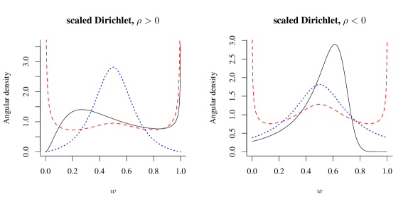
Figure 1: Angular density of the scaled extremal Dirichlet model. Left panel: $\rho=4/5$ and $\boldsymbol{\alpha}=(2,1/2)$ (black full), $\rho=1/4$ and $\boldsymbol{\alpha}=(1/10,1/10)$ (red dashed), $\rho=1/4$ and $\boldsymbol{\alpha}=(1/2,1/2)$ (blue dotted). Right panel: $\rho=-1/4$ and $\boldsymbol{\alpha}=(2,1/2)$ (black full), $\boldsymbol{\alpha}=(2/5,2/5)$ (red dashed) and $\boldsymbol{\alpha}=(1/2,1/2)$ (blue dotted).

5.1.  Angular density

The first property worth noting is that the positive and negative scaled extremal Dirichlet models are closed under marginalization. Indeed, letting $x_{i}\to 0$ for some arbitrary $1\leq i\leq d$, we can easily derive from Lemma 2 that for any $\boldsymbol{\alpha}>\boldsymbol{0}_{d}$, $\rho>0$, and any $\boldsymbol{x}\in\mathbb{R}_{+}^{d}$, $\ell^{\mathrm{pD}}(\boldsymbol{x};\rho,\boldsymbol{\alpha})\to\ell^{\mathrm{pD}}(\boldsymbol{x}_{-i};\rho,\boldsymbol{\alpha}_{-i})$ as $x_{i}\to 0$, where for any $\boldsymbol{y}\in\mathbb{R}^{d}$, $\boldsymbol{y}_{-i}$ denotes the vector $(y_{1},\dots,y_{i-1},y_{i+1},\dots,y_{d})$. Similarly, for any $1\leq i\leq d$, $\boldsymbol{\alpha}>\boldsymbol{0}_{d}$, $0<\rho<\min(\alpha_{1},\dots,\alpha_{d})$, and any $\boldsymbol{x}\in\mathbb{R}_{+}^{d}$, $\ell^{\mathrm{nD}}(\boldsymbol{x};\rho,\boldsymbol{\alpha})\to\ell^{\mathrm{nD}}(\boldsymbol{x}_{-i};\rho,\boldsymbol{\alpha}_{-i})$ as $x_{i}\to 0$.

Since none of the scaled extremal Dirichlet models places mass on the vertices or facets of the simplex $\mathbb{S}_{d}$ when $\rho\neq 0$, the density of the angular measure $\sigma_{d}$ completely characterizes the stable tail dependence function and hence also the associated extreme-value copula. This so-called angular density of the scaled extremal Dirichlet models is given below and derived in D.

Proposition 5.

Let $d\geq 2$ and set $\alpha_{1},\dots,\alpha_{d}>0$ and $\bar{\alpha}=\alpha_{1}+\cdots+\alpha_{d}$. For any $\rho>-\min(\alpha_{1},\dots,\alpha_{d})$, let also $\boldsymbol{c}(\boldsymbol{\alpha},\rho)=(c(\alpha_{1},\rho),\dots,c(\alpha_{d},\rho))$, where $c(\alpha,\rho)$ is as in Definition 1. Then for any $-\min(\alpha_{1},\dots,\alpha_{d})<\rho<\infty$, $\rho\neq 0$, the angular density of the scaled extremal Dirichlet model with parameters $\rho>0$ and $\boldsymbol{\alpha}$ is given, for all $\boldsymbol{w}\in\mathbb{S}_{d}$, by

$$h^{\mathrm{D}}(\boldsymbol{w};\rho,\boldsymbol{\alpha})=\frac{\Gamma(\bar{\alpha}+\rho)}{d|\rho|^{d-1}\prod_{i=1}^{d}\Gamma(\alpha_{i})}\left[\sum_{j=1}^{d}\left\{c(\boldsymbol{\alpha}_{j},\rho)w_{j}\right\}^{1/\rho}\right]^{-\rho-\bar{\alpha}}\prod_{i=1}^{d}\{c(\alpha_{i},\rho)\}^{\alpha_{i}/\rho}w_{i}^{\alpha_{i}/\rho-1}.$$

The angular density of the positive scaled extremal Dirichlet model with parameters $\rho>0$ and $\boldsymbol{\alpha}$ is given, for all $\boldsymbol{w}\in\mathbb{S}_{d}$, by $h^{\mathrm{pD}}(\boldsymbol{w};\rho,\boldsymbol{\alpha})=h^{\mathrm{D}}(\boldsymbol{w};\rho,\boldsymbol{\alpha})$, while the angular density of the negative scaled extremal Dirichlet model with parameters $0<\rho<\min(\alpha_{1},\dots,\alpha_{d})$ and $\boldsymbol{\alpha}$ is given, for all $\boldsymbol{w}\in\mathbb{R}_{+}^{d}$, by $h^{\mathrm{nD}}(\boldsymbol{w};\rho,\boldsymbol{\alpha})=h^{\mathrm{D}}(\boldsymbol{w};-\rho,\boldsymbol{\alpha})$.

From Proposition 5, it is easily seen that when $\boldsymbol{\alpha}=\boldsymbol{1}_{d}$, the angular density $h^{\mathrm{pD}}$ reduces, for any $\rho>0$ and $\boldsymbol{w}\in\mathbb{S}_{d}$, to the angular density of the symmetric negative logistic model; see, e.g., Section 4.2 in [7]. In general, the angular density $h^{\mathrm{pD}}$ is not symmetric unless $\boldsymbol{\alpha}=\alpha\boldsymbol{1}_{d}$.

The positive scaled Dirichlet model can thus be viewed as a new asymmetric generalization of the negative logistic model which does not place any mass on the vertices or facets of $\mathbb{S}_{d}$, unless at independence or comonotonicity, i.e., when $\rho\to\infty$ and $\rho\to 0$, respectively. Furthermore, $h^{\mathrm{pD}}$ can also be interpreted as a generalization of the Coles–Tawn extremal Dirichlet model. Indeed, $h^{\mathrm{pD}}(\boldsymbol{x};1,\boldsymbol{\alpha})$ is precisely the angular density of the latter model given, e.g., in Equation (3.6) in [7]. Similarly, the negative scaled extremal Dirichlet model is a new asymmetric generalization of Gumbel’s logistic model [16]. Indeed, when $\boldsymbol{\alpha}=\boldsymbol{1}_{d}$, $h^{\mathrm{nD}}$ simplifies to the logistic angular density, given, e.g., on p. 381 in [7].

Figures 1 and 2 illustrate the various shapes of $h^{\mathrm{pD}}$ and $h^{\mathrm{nD}}$ that obtain through various choices of $\boldsymbol{\alpha}$ and $\rho$. The asymmetry when $\boldsymbol{\alpha}\neq\alpha\boldsymbol{1}_{d}$ is clearly apparent. For the same value of $\rho$, the shapes of the angular density can be quite different depending on $\boldsymbol{\alpha}$. In view of the aforementioned closure of both the positive and negative scaled extremal Dirichlet models under marginalization, this means that these models are able to capture strong dependence in some pairs of variables (represented by a mode close to $1/2$ of the angular density) and at the same time weak dependence in others pairs (represented by a bathtub shape).

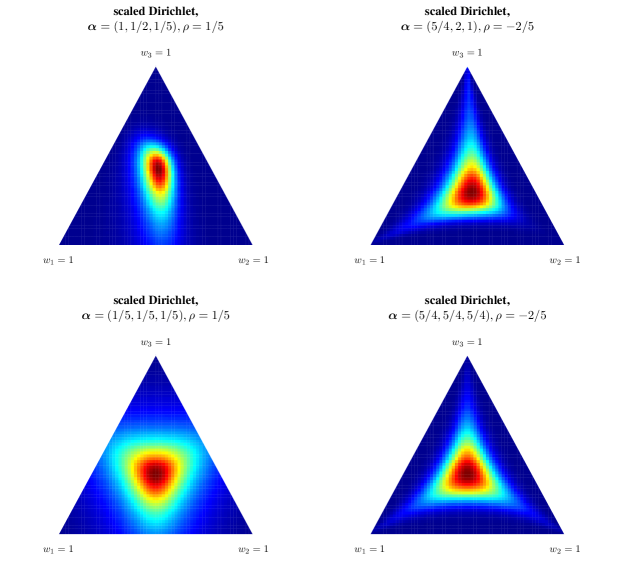
Figure 2: Angular density of the scaled extremal Dirichlet model with $\boldsymbol{\alpha}=(1,1/2,1/5),\rho=1/5$ (top left) and $\boldsymbol{\alpha}=(1/5,1/5,1/5),\rho=1/5$ (bottom left), $\boldsymbol{\alpha}=(5/4,2,1)$, $\rho=-2/5$ (top right) and $\boldsymbol{\alpha}=(5/4,5/4,5/4),\rho=-2/5$ (bottom right). The colors correspond to log density values and range from red (high density) to blue (low density).

5.2.  The bivariate case

When $d=2$, the stable tail dependence functions of the positive and negative scaled extremal Dirichlet models have a closed-form expression in terms of the incomplete beta function given, for any $t\in(0,1)$ and $\alpha_{1},\alpha_{2}>0$, by

$$\mathrm{B}(t;\alpha_{1},\alpha_{2})=\int_{0}^{t}x^{\alpha_{1}-1}(1-x)^{\alpha_{2}-1}{\,\textrm{d}}x.$$

When $t=1$, this integral is the beta function, viz. $\mathrm{B}(\alpha_{1},\alpha_{2})=\Gamma(\alpha_{1})\Gamma(\alpha_{2})/\Gamma(\alpha_{1}+\alpha_{2})$. A direct calculation yields the corresponding Pickands dependence function, for any $t\in[0,1]$, $\mathrm{A}^{\mathrm{pD}}(t;\rho,\alpha_{1},\alpha_{2})=\ell^{\mathrm{pD}}(1-t,t;\rho,\alpha_{1},\alpha_{2})$, i.e.,

$$\mathrm{A}^{\mathrm{pD}}(t;\rho,\alpha_{1},\alpha_{2})=\frac{(1-t)}{\mathrm{B}(\alpha_{2},\alpha_{1}+\rho)}\mathrm{B}\left[\frac{\left\{c(\alpha_{2},\rho)(1-t)\right\}^{1/\rho}}{\left\{c(\alpha_{2},\rho)(1-t)\right\}^{1/\rho}+\left\{c(\alpha_{1},\rho)t\right\}^{1/\rho}};\alpha_{2},\alpha_{1}+\rho\right]\\ +\frac{t}{\mathrm{B}(\alpha_{1},\alpha_{2}+\rho)}\mathrm{B}\left[\frac{\left\{c(\alpha_{1},\rho)t\right\}^{1/\rho}}{\left\{c(\alpha_{2},\rho)(1-t)\right\}^{1/\rho}+\left\{c(\alpha_{1},\rho)t\right\}^{1/\rho}};\alpha_{1},\alpha_{2}+\rho\right].$$

When $\alpha_{1}=\alpha_{2}=1$, $\mathrm{A}^{\mathrm{pD}}$ becomes the Pickands dependence function of the Galambos copula, viz. $\mathrm{A}^{\mathrm{pD}}(t;\rho,1,1)=1-\bigl{\{}t^{-1/\rho}+(1-t)^{-1/\rho}\bigr{\}}^{-\rho}$, as expected given that the positive scaled extremal Dirichlet model becomes the symmetric negative logistic model in this case.

Similarly, for any $t\in[0,1]$, the Pickands dependence function $\mathrm{A}^{\mathrm{nD}}(t;\rho,\alpha_{1},\alpha_{2})=\ell^{\mathrm{nD}}(1-t,t;\rho,\alpha_{1},\alpha_{2})$ equals

$$\mathrm{A}^{\mathrm{nD}}(t;\rho,\alpha_{1},\alpha_{2})=\frac{(1-t)}{\mathrm{B}(\alpha_{1}-\rho,\alpha_{2})}\mathrm{B}\left[\frac{\left\{(1-t)c(\alpha_{2},-\rho)\right\}^{1/\rho}}{\left\{tc(\alpha_{1},-\rho)\right\}^{1/\rho}+\left\{(1-t)c(\alpha_{2},-\rho)\right\}^{1/\rho}};\alpha_{1}-\rho,\alpha_{2}\right]\\ +\frac{t}{\mathrm{B}(\alpha_{2}-\rho,\alpha_{1})}\mathrm{B}\left[\frac{\left\{tc(\alpha_{1},-\rho)\right\}^{1/\rho}}{\left\{tc(\alpha_{1},-\rho)\right\}^{1/\rho}+\left\{(1-t)c(\alpha_{2},-\rho)\right\}^{1/\rho}};\alpha_{2}-\rho,\alpha_{1}\right].$$

When $\alpha_{1}=\alpha_{2}=1$, $\mathrm{A}^{\mathrm{nD}}$ simplifies to the stable tail dependence function of the Gumbel extreme-value copula, viz. $\mathrm{A}^{\mathrm{nD}}(t;\rho,1,1)=\bigl{\{}t^{1/\rho}+(1-t)^{1/\rho}\bigr{\}}^{\rho}$. This again confirms that the negative scaled extremal Dirichlet model becomes the symmetric logistic model when $\alpha_{1}=\alpha_{2}=1$. The Pickands dependence functions $\mathrm{A}^{\mathrm{pD}}$ and $\mathrm{A}^{\mathrm{nD}}$ are illustrated in Figure 3, for the same choices of parameters and the corresponding angular density shown in Figure 1.

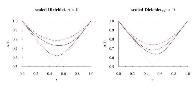
Figure 3: Pickands dependence function of the scaled extremal Dirichlet model. Left panel: $\rho=4/5$ and $\boldsymbol{\alpha}=(2,1/2)$ (black full), $\rho=1/4$ and $\boldsymbol{\alpha}=(1/10,1/10)$ (red dashed), $\rho=1/4$ and $\boldsymbol{\alpha}=(1/2,1/2)$ (blue dotted). Right panel: $\rho=-1/4$ and $\boldsymbol{\alpha}=(2,1/2)$ (black full), $\boldsymbol{\alpha}=(2/5,2/5)$ (red dashed) and $\boldsymbol{\alpha}=(1/2,1/2)$ (blue dotted).

The above formulas for $\mathrm{A}^{\mathrm{pD}}$ and $\mathrm{A}^{\mathrm{nD}}$ now easily lead to expressions for their upper tail dependence coefficients. Recall that for an arbitrary bivariate copula $C$, the lower and upper tail dependence coefficients of [25] are given by

$$\lambda_{\ell}(C)=\lim_{u\to 0}\frac{C(u,u)}{u},\quad\lambda_{u}(C)=2-\lim_{u\to 1}\frac{C(u,u)-1}{u-1}=\lim_{u\to 0}\frac{\hat{C}(u,u)}{u},$$

where $\hat{C}$ is the survival copula of $C$, provided these limits exist. When $C$ is bivariate extreme-value with Pickands dependence function $\mathrm{A}$, it follows easily from (4) that $\lambda_{\ell}(C)=0$ and $\lambda_{u}(C)=2-2\mathrm{A}(1/2)$.

Now suppose that $C^{\mathrm{pD}}_{\rho,\boldsymbol{\alpha}}$ is a bivariate extreme-value copula with positive scaled extremal Dirichlet Pickands dependence function $\mathrm{A}^{\mathrm{pD}}$ and parameters $\rho>0$ and $\alpha_{1},\alpha_{2}>0$. Then

$$\lambda_{u}(C^{\mathrm{pD}}_{\rho,\boldsymbol{\alpha}})=2-\frac{1}{\mathrm{B}(\alpha_{2},\alpha_{1}+\rho)}\mathrm{B}\left\{\frac{c(\alpha_{2},\rho)^{1/\rho}}{c(\alpha_{2},\rho)^{1/\rho}+c(\alpha_{1},\rho)^{1/\rho}};\alpha_{2},\alpha_{1}+\rho\right\}\\ -\frac{1}{\mathrm{B}(\alpha_{1},\alpha_{2}+\rho)}\mathrm{B}\left\{\frac{c(\alpha_{1},\rho)^{1/\rho}}{c(\alpha_{2},\rho)^{1/\rho}+c(\alpha_{1},\rho)^{1/\rho}};\alpha_{1},\alpha_{2}+\rho\right\}.$$ (8)

Similarly, if $C^{\mathrm{nD}}_{\rho,\boldsymbol{\alpha}}$ is a bivariate extreme-value copula with negative scaled extremal Dirichlet Pickands dependence function $\mathrm{A}^{\mathrm{nD}}$ and parameters $\alpha_{1},\alpha_{2}>0$ and $0<\rho<\min(\alpha_{1},\alpha_{2})$, then

$$\lambda_{u}(C^{\mathrm{nD}}_{\rho,\boldsymbol{\alpha}})=2-\frac{1}{\mathrm{B}(\alpha_{1}-\rho,\alpha_{2})}\mathrm{B}\left\{\frac{c(\alpha_{2},-\rho)^{1/\rho}}{c(\alpha_{1},-\rho)^{1/\rho}+c(\alpha_{2},-\rho)^{1/\rho}};\alpha_{1}-\rho,\alpha_{2}\right\}\\ +\frac{1}{\mathrm{B}(\alpha_{2}-\rho,\alpha_{1})}\mathrm{B}\left\{\frac{c(\alpha_{1},-\rho)^{1/\rho}}{c(\alpha_{1},-\rho)^{1/\rho}+c(\alpha_{2},-\rho)^{1/\rho}};\alpha_{2}-\rho,\alpha_{1}\right\}.$$ (9)

In the symmetric case $\alpha_{1}=\alpha_{2}\equiv\alpha$, Expressions (8) and (9) simplify to

$$\lambda_{u}(C^{\mathrm{pD}}_{\rho,\boldsymbol{\alpha}})=2-\frac{2}{\mathrm{B}(\alpha,\alpha+\rho)}\mathrm{B}\left(\frac{1}{2};\alpha,\alpha+\rho\right),\quad\lambda_{u}(C^{\mathrm{nD}}_{\rho,\boldsymbol{\alpha}})=2-\frac{2}{\mathrm{B}(\alpha-\rho,\alpha)}\mathrm{B}\left(\frac{1}{2};\alpha-\rho,\alpha\right).$$

Formulas (8) and (9) lead directly to expressions for the tail dependence coefficients of Liouville copulas. This is because if $C\in\mathcal{M}(C_{0})$, where $C_{0}$ is an extreme-value copula with Pickands tail dependence function $\mathrm{A}_{0}$, $\lambda_{u}(C)=2-2\mathrm{A}_{0}(1/2)$ [29, Proposition 7.51]. Similarly, if $\hat{C}\in\mathcal{M}(C_{0}^{*})$, where $C^{*}_{0}$ is an extreme-value copula with Pickands tail dependence function $\mathrm{A}^{*}_{0}$, $\lambda_{\ell}(C)=2-2\mathrm{A}^{*}_{0}(1/2)$. The following corollary is thus an immediate consequence of Corollaries 1 and 2.

Corollary 3.

Suppose that $C$ is the survival copula of a Liouville random vector $R\boldsymbol{D}_{\boldsymbol{\alpha}}$ with parameters $\boldsymbol{\alpha}>0$ and a radial part $R$ such that $\Pr(R\leq 0)=0$. Then the following statements hold.

1. If $R\in\mathcal{M}(\Phi_{\rho})$ for some $\rho>0$, $\lambda_{\ell}(C)=\lambda_{u}(C^{\mathrm{pD}}_{\rho,\boldsymbol{\alpha}})$ is given by Equation 8.

2. If $R\in\mathcal{M}(\Lambda)$ or $R\in\mathcal{M}(\Psi_{\rho})$ for some $\rho>0$, $\lambda_{\ell}(C)=0$.

3. If $1/R\in\mathcal{M}(\Phi_{\rho})$ for some $0<\rho<\alpha_{1}\wedge\alpha_{2}$, $\lambda_{u}(C)=\lambda_{u}(C^{\mathrm{nD}}_{\rho,\boldsymbol{\alpha}})$ is given by Equation 9.

4. If $1/R\in\mathcal{M}(\Phi_{\rho})$ for $\rho>\alpha_{1}\wedge\alpha_{2}$ or if $\mathrm{E}({1/R^{\beta}})<\infty$ for $\beta>\alpha_{1}\vee\alpha_{2}$, $\lambda_{u}(C)=0$.

The role of the parameters $\boldsymbol{\alpha}$ and $\rho$ is best explained if we consider the reparametrization $\Delta_{\alpha}=|\alpha_{1}-\alpha_{2}|$ and $\Sigma_{\alpha}=\alpha_{1}+\alpha_{2}$. As is the case for the Dirichlet distribution, the level of dependence is higher for large values of $\Sigma_{\alpha}$. Furthermore, $\lambda_{u}$ is monotonically decreasing in $\rho$. Higher levels of extremal asymmetry, as measured by departures from the diagonal on the copula scale, are governed by both $\Sigma_{\alpha}$ and $\Delta_{\alpha}$. The larger $\Sigma_{\alpha}$, the lower the asymmetry. Likewise, the larger $\Delta_{\alpha}$, the larger the asymmetry. Contrary to the case of extremal dependence, the behavior in $\rho$ is not monotone. For the negative scaled extremal Dirichlet model, asymmetry is maximal when $\rho\approx\alpha_{1}\wedge\alpha_{2}$. When $\Sigma_{\alpha}$ is small, smaller values of $\rho$ induce larger asymmetry, but this is not the case for larger values of $\Sigma_{\alpha}$ where the asymmetry profile is convex with a global maximum attained for larger values of $\rho$.

Appendix 6. : de Haan representation and simulation algorithms

Random samples from the scaled extremal Dirichlet model can be drawn efficiently using the algorithms recently developed in [10]. We first derive the so-called de Haan representation in Section 6.1 and adapt the algorithms from [10] to the present setting in Section 6.2.

6.1.  de Haan representation

First, introduce the following family of univariate distributions, which we term the scaled Gamma family and denote by $\mathsf{sGa}(a,b,c)$. It has three parameters $a,c>0$ and $b\neq 0$ and a density given, for all $x>0$, by

$$f(x;a,b,c)=\frac{|b|}{\Gamma(c)}a^{-bc}x^{bc-1}\exp\left\{-\left(\frac{x}{a}\right)^{b}\right\}.$$ (10)

Observe that when $Z\sim\mathsf{Ga}(c,1)$ is a Gamma variable with shape parameter $c>0$ and scaling parameter $1$, $Y\stackrel{{\scriptstyle\mbox{\tiny d}}}{{=}}aZ^{1/b}$ is scaled Gamma $\mathsf{sGa}(a,b,c)$. Consequently, ${\mathrm{E}}\left(Y\right)=a\Gamma(c+1/b)/\Gamma(c)<\infty$ provided that $b<-1/c$. The scaled Gamma family includes several well-known distributions as special cases, notably the Gamma when $b=1$, the Weibull when $c=1$ and $b>0$, the inverse Gamma when $b=-1$, and the Fréchet when $c=1$ and $b<0$. When $b>0$, the scaled Gamma is the generalized Gamma distribution of [41], albeit in a different parametrization.

Now consider the parameters $\boldsymbol{\alpha}=(\alpha_{1},\dots,\alpha_{d})$ with $\boldsymbol{\alpha}>\boldsymbol{0}_{d}$ and $\rho>-\min(\alpha_{1},\ldots,\alpha_{d})$, $\rho\neq 0$. Let $\boldsymbol{V}$ be a random vector with independent scaled Gamma margins $V_{i}\sim\mathsf{sGa}\{1/c(\alpha_{i},\rho),1/\rho,\alpha_{i}\}$, where for $\alpha>0$, $c(\alpha,\rho)=\Gamma(\alpha+\rho)/\Gamma(\alpha)$ as in Definition 1. If $\boldsymbol{Z}$ is a random vector with independent Gamma margins $Z_{i}\sim\mathsf{Ga}(\alpha_{i},1)$ then for all $i=1,\dots,d$, $V_{i}\stackrel{{\scriptstyle\mbox{\tiny d}}}{{=}}Z_{i}^{\rho}/c(\alpha_{i},\rho)$. Furthermore, recall that $\|\boldsymbol{Z}\|\sim\mathsf{Ga}(\bar{\alpha},1)$ is independent of $\boldsymbol{Z}/\|\boldsymbol{Z}\|$, which has the same distribution as the Dirichlet vector $\boldsymbol{D}_{\boldsymbol{\alpha}}=(D_{1},\dots,D_{d})$. One thus has, for all $\boldsymbol{x}\in\mathbb{R}_{+}^{d}$,

$$\mathrm{E}\left\{\max_{1\leq i\leq d}(x_{i}V_{i})\right\}=\mathrm{E}\left[\max_{1\leq i\leq d}\left\{\frac{x_{i}Z_{i}^{\rho}}{c(\alpha_{i},\rho)}\right\}\right]={\mathrm{E}}\left(\|\boldsymbol{Z}\|^{\rho}\right)\mathrm{E}\left[\max_{1\leq i\leq d}\left\{\frac{x_{i}D_{i}^{\rho}}{c(\alpha_{i},\rho)}\right\}\right]=\ell^{\mathrm{D}}(\boldsymbol{x};\rho,\boldsymbol{\alpha}),$$ (11)

where $\ell^{\mathrm{D}}$ is as in Definition 1, given that ${\mathrm{E}}\left(\|\boldsymbol{Z}\|^{\rho}\right)=c(\bar{\alpha},\rho)$.

When $\rho=1$, the positive scaled Dirichlet extremal model becomes the Coles–Tawn Dirichlet extremal model, $V_{i}\sim\mathsf{Ga}(\alpha_{i},1)$ and Equation 11 reduces to the representation derived in [37]. When $\boldsymbol{\alpha}=\boldsymbol{1}_{d}$, $\ell^{\mathrm{D}}$ becomes the stable tail dependence function of the negative logistic model, $V_{i}$ is Weibull and Equation 11 is the representation in Appendix A.2.4 of [10]. Similarly, when $\rho<0$ and $\boldsymbol{\alpha}=\boldsymbol{1}_{d}$, the negative scaled Dirichlet extremal model becomes the logistic model, $V_{i}$ is Fréchet and Equation 11 is the representation in Appendix A.2.4 of [10]. The requirement that $\rho>-\min(\alpha_{1},\dots,\alpha_{d})$ ensures that the expectation of $V_{i}$ is finite for all $i\in\{1,\ldots,d\}$.

Equation 11 implies that the max-stable random vector $\boldsymbol{Y}$ with unit Fréchet margins and extreme-value copula with stable tail dependence function $\ell^{\mathrm{D}}(\cdot;\rho,\boldsymbol{\alpha})$ admits the de Haan [9] spectral representation

$$\boldsymbol{Y}\stackrel{{\scriptstyle\mbox{\tiny d}}}{{=}}\max_{k\in\mathbb{N}}\zeta_{k}\boldsymbol{V}_{k},$$ (12)

where $\mathcal{Z}=\{\zeta_{k}\}_{k=1}^{\infty}$ is a Poisson point process on $(0,\infty)$ with intensity $\zeta^{-2}{\,\textrm{d}}\zeta$ and $\boldsymbol{V}_{k}$ is an i.i.d. sequence of random vectors independent of $\mathcal{Z}$. Furthermore, the univariate margins of $\boldsymbol{V}_{k}$ are independent and such that $V_{kj}\sim\mathsf{sGa}\{1/c(\alpha_{j},\rho),1/\rho,\alpha_{j}\}$ for $j=1,\dots,d$ with ${\mathrm{E}}\left(\boldsymbol{V}_{k}\right)=\boldsymbol{1}_{d}$ for all $k\in{\mathbb{N}}$.

6.2.  Unconditional simulation

The de Haan representation (12) offers, among other things, an easy route to unconditional simulation of max-stable random vectors that follow the scaled Dirichlet extremal model, as laid out in [10] in the more general context of max-stable processes. To see how this work applies in the present setting, fix an arbitrary $j_{0}\in\{1,\dots,d\}$ and recall that the $j_{0}$th extremal function $\phi^{+}_{j_{0}}$ is given, almost surely, as $\zeta_{k}\boldsymbol{V}_{k}$ such that $Y_{j_{0}}=\zeta_{k}V_{kj_{0}}$. From eq. 12 and Proposition 1 in [10] it then directly follows that $\phi^{+}_{j_{0}}/Y_{j_{0}}\stackrel{{\scriptstyle\mbox{\tiny d}}}{{=}}(W_{j_{0}1}/W_{j_{0}j_{0}},\ldots,W_{j_{0}d}/W_{j_{0}j_{0}})$, where $\boldsymbol{W}_{j_{0}}=(W_{j_{0}1},\dots,W_{j_{0}d})$ is a random vector with density given, for all $\boldsymbol{x}\in\mathbb{R}_{+}^{d}$, by

$$\frac{|1/\rho|}{\Gamma(\alpha_{j_{0}})}c(\alpha_{j_{0}},\rho)^{\alpha_{j_{0}}/\rho}x_{j_{0}}^{\alpha_{j_{0}}/\rho}\exp\left[-\{c(\alpha_{j_{0}},\rho)x_{j_{0}}\}^{1/\rho}\right]\times\prod_{j=1,j\neq j_{0}}^{d}\frac{|1/\rho|}{\Gamma(\alpha_{j})}c(\alpha_{j},\rho)^{\alpha_{j}/\rho}x_{j}^{\alpha_{j}/\rho-1}\exp\left[-\{c(\alpha_{j},\rho)x_{j}\}^{1/\rho}\right].$$

This means that the components of $\boldsymbol{W}_{j_{0}}$ are independent and such that $W_{j_{0}j}\sim\mathsf{sGa}\{1/c(\alpha_{j},\rho),1/\rho,\alpha_{j}\}$ when $j\neq j_{0}$ and $W_{j_{0}j_{0}}\sim\mathsf{sGa}\{1/c(\alpha_{j_{0}},\rho),1/\rho,\alpha_{j_{0}}+\rho\}$. In other words, $W_{j_{0}j_{0}}\sim Z_{j_{0}}^{\rho}/c(\alpha_{j_{0}},\rho)$ where $Z_{j_{0}}\sim\mathsf{Ga}(\alpha_{j_{0}}+\rho,1)$, while for all $j\neq j_{0}$, $W_{j_{0}j}\stackrel{{\scriptstyle\mbox{\tiny d}}}{{=}}Z_{j}^{\rho}/c(\alpha_{j},\rho)$ where $Z_{j}\sim\mathsf{Ga}(\alpha_{j},1)$.

The exact distribution of $\phi^{+}_{j_{0}}/Y_{j_{0}}$ given above now allows for an easy adaptation of the algorithms in [10]. To draw an observation from the extreme-value copula with the scaled Dirichlet stable tail dependence function $\ell^{\mathrm{D}}$ with parameters $\boldsymbol{\alpha}>\boldsymbol{0}_{d}$ and $\rho>-\min(\alpha_{1},\dots,\alpha_{d})$, $\rho\neq 0$, one can follow Algorithms 1 and 2 below. The first procedure corresponds to Algorithm 1 in [10] and relies on [36]; the second is an adaptation of Algorithm 2 in [10].

Algorithm 1 Exact simulations from the extreme-value copula based on spectral densities.

1:Simulate $E\sim\mathsf{Exp}(1)$ .

2:Set $\boldsymbol{Y}=\boldsymbol{0}$.

3:while $1/E>\min(Y_{1},\dots,Y_{d})$ do

4:    Simulate $J$ from the uniform distribution on $\{1,\dots,d\}$.

5:    Simulate independent $Z_{j}\sim\mathsf{Ga}(\alpha_{j},1)$ for $j\in\{1,\ldots,d\}\setminus J$ and $Z_{J}\sim\mathsf{Ga}(\alpha_{J}+\rho,1)$.

6:    Set $W_{j}\leftarrow Z_{j}^{\rho}/c(\alpha_{j},\rho)$, $j=1,\dots,d$.

7:    Set $\boldsymbol{S}\leftarrow\boldsymbol{W}/\|\boldsymbol{W}\|$.

8:    Update $\boldsymbol{Y}\leftarrow\max\{\boldsymbol{Y},d\boldsymbol{S}/E\}$.

9:    Simulate $E^{*}\sim\mathsf{Exp}(1)$ and update $E\leftarrow E+E^{*}$.

10:return $\boldsymbol{U}=\exp(-1/\boldsymbol{Y})$.

Algorithm 2 Exact simulations based on sequential sampling of the extremal functions.

1:Simulate $Z_{1}\sim\mathsf{Ga}(\alpha_{1}+\rho,1)$ and $Z_{j}\sim\mathsf{Ga}(\alpha_{j},1)$, $j=2,\dots,d$.

2:Compute $\boldsymbol{W}$ where $W_{j}\leftarrow Z_{j}^{\rho}/c(\alpha_{j},\rho)$, $j=1,\dots,d$.

3:Simulate $E_{1}\sim\mathsf{Exp}(1)$.

4:Set $\boldsymbol{Y}\leftarrow\boldsymbol{W}/(W_{1}E_{1})$.

5:for $k=2,\dots,d$ do

6:    Simulate $E_{k}\sim\mathsf{Exp}(1)$.

7:    while $1/E_{k}>Y_{k}$ do

8:         Simulate independent $Z_{k}\sim\mathsf{Ga}(\alpha_{k}+\rho,1)$ and $Z_{j}\sim\mathsf{Ga}(\alpha_{j},1)$, $j=1,\ldots,d,j\neq k$ .

9:         Set $\boldsymbol{W}=(W_{1},\ldots,W_{d})$ where $W_{j}\leftarrow Z_{j}^{\rho}/c(\alpha_{j},\rho)$, $j=1,\dots,d$.

10:         if $W_{i}/(W_{k}E_{k})<Y_{i}$ for all $i=1,\dots,k-1$ then

11:             Update $\boldsymbol{Y}\leftarrow\max\{\boldsymbol{Y},\boldsymbol{W}/(W_{k}E_{k})\}$.          

12:         Simulate $E^{*}\sim\mathsf{Exp}(1)$ and update $E_{k}\leftarrow E_{k}+E^{*}$.     

13:return $\boldsymbol{U}=\exp(-1/\boldsymbol{Y})$.

Note that $\boldsymbol{S}$ obtained in Step 7 of Algorithm 1 has the angular distribution $\sigma_{d}$ of $\ell^{\mathrm{D}}$; see Theorem 1 in [10]. Similar algorithms for drawing samples from the angular distribution of the extremal logistic and Dirichlet models were obtained in [3]. Algorithm 2 requires a lower number of simulations and is more efficient on average, cf. [10]. Both algorithms are easily implemented using the function rmev in the mev package within the R Project for Statistical Computing [34], which returns samples of max-stable scaled extremal Dirichlet vectors with unit Fréchet margins, i.e., $\boldsymbol{Y}$ in Algorithms 1 and 2.

Appendix 7. : Estimation

The scaled extremal Dirichlet model can be used to model dependence between extreme events. To this end, several schemes can be envisaged. For example, one can consider the block-maxima approach, given that max-stable distributions are the most natural for such data. Another option is peaks-over-threshold models. Yet another alternative, used in [13] for the Brown–Resnick model, is to approximate the conditional distribution of a random vector with unit Fréchet margins given that the $j_{0}$th component exceeds a large threshold by the distribution of $\phi^{+}_{j_{0}}/Y_{j_{0}}$ discussed in Section 6.2.

Here, we focus on the multivariate tail model of [28]; see also Section 16.4 in [29]. To this end, let $\boldsymbol{X}_{1},\dots,\boldsymbol{X}_{n}$ be a random sample from some unknown multivariate distribution $H$ with continuous univariate margins which is assumed to be in the maximum domain of attraction of a multivariate extreme-value distribution $H_{0}$. To model the tail of $H$, its margins $F_{j}$, $j=1,\dots,d$ can first be approximated using the univariate peaks-over-threshold method. For all $x$ above some high threshold $u_{j}$, one then has

$$F_{j}(x)\approx\tilde{F}_{j}(x;\eta_{j},\xi_{j})=1-\nu_{j}\left(1+\xi_{j}\frac{(x-u_{j})}{\eta_{j}}\right)_{+}^{-1/\xi_{j}},$$ (13)

where $\nu_{j}=1-F_{j}(u_{j})$, and $\eta_{j}>0$ and $\xi_{j}$ are the parameters of the generalized Pareto distribution. Furthermore, for $\boldsymbol{w}$ sufficiently close to $\boldsymbol{1}_{d}$, the copula of $H$ can be approximated by the extreme-value copula $C_{0}$ of $H_{0}$, so that, for $\boldsymbol{x}\geq\boldsymbol{u}$, $H(\boldsymbol{x})\approx\tilde{H}(\boldsymbol{x})=C_{0}\{\tilde{F}_{1}(x_{1}),\dots,\tilde{F}_{d}(x_{d})\}$. The parameters of this multivariate tail model, i.e., the parameters $\boldsymbol{\theta}$ of the stable tail dependence function $\ell_{0}$ of $C_{0}$ as well as the marginal parameters $\boldsymbol{\nu}$, $\boldsymbol{\eta}$ and $\boldsymbol{\xi}$ can be estimated using likelihood methods; this allows, e.g., for Bayesian inference, generalized additive modeling of the parameters and model selection based on likelihood-ratio tests. For a comprehensive review of likelihood inference methods for extremes, see, e.g., [22].

The multivariate tail model can be fitted in low-dimensions using the censored likelihood $L(\boldsymbol{X};\boldsymbol{\nu},\boldsymbol{\eta},\boldsymbol{\xi},\boldsymbol{\theta})=\prod_{i=1}^{n}L_{i}(\boldsymbol{X}_{i};\boldsymbol{\nu},\boldsymbol{\eta},\boldsymbol{\xi},\boldsymbol{\theta})$, where for $i=1,\dots,n$,

$$L_{i}(\boldsymbol{X}_{i};\boldsymbol{u},\boldsymbol{\nu},\boldsymbol{\eta},\boldsymbol{\xi},\boldsymbol{\theta})=\left.\frac{\partial^{m_{i}}\tilde{H}(y_{1},\dots,y_{d})}{\partial y_{j_{1}}\dotsm\partial y_{j_{m_{i}}}}\right|_{\boldsymbol{y}=\max(\boldsymbol{X}_{i},\boldsymbol{u})}=\left.\frac{\partial^{m_{i}}\exp\{-\ell_{0}(1/\boldsymbol{y})\}}{\partial y_{j_{1}}\dotsm\partial y_{j_{m_{i}}}}\right|_{\boldsymbol{y}=t\{\max(\boldsymbol{X}_{i},\boldsymbol{u})\}}\prod_{k=1}^{m_{i}}J_{j_{k}}(X_{ij_{k}})$$ (14)

In this expression, the indices $j_{1},\dots,j_{m_{i}}$ are those of the components of $\boldsymbol{X}_{i}$ exceeding the thresholds $\boldsymbol{u}$ and for $\boldsymbol{x}\geq\boldsymbol{u}$, $t(\boldsymbol{x})=(t_{1}(x_{1}),\dots,t_{d}(x_{d}))$, where for $j=1,\dots,d$,

$$t_{j}(x_{j})=-\frac{1}{\log\{\tilde{F}_{j}(x_{j};\eta_{j},\xi_{j})\}},\qquad J_{j}(x_{j})=\frac{\nu_{j}}{\eta_{j}}\left(1+\xi_{j}\frac{(x_{j}-u_{j})}{\eta_{j}}\right)^{-1/\xi_{j}-1}\!\!\!\frac{1}{[\log\{\tilde{F}_{j}(x_{j};\eta_{j},\xi_{j})\}]^{2}\tilde{F}_{j}(x_{j};\eta_{j},\xi_{j})}.$$ (15)

The censored likelihood $L(\boldsymbol{X};\boldsymbol{\nu},\boldsymbol{\eta},\boldsymbol{\xi},\boldsymbol{\theta})$ can be maximized either over all parameters at once, or the marginal parameters $\boldsymbol{\nu}$, $\boldsymbol{\eta}$ and $\boldsymbol{\xi}$ can be estimated from each univariate margin separately, so that only the estimate of $\boldsymbol{\theta}$ is obtained through maximizing $L$. When $d$ is large, one can also maximize the likelihood in [40] that uses the tail approximation $\bar{H}(\boldsymbol{x})\approx 1-\ell(1/\boldsymbol{x})$. In either case, $\ell_{0}$ and the higher-order partial derivatives of $\ell_{0}(1/\boldsymbol{x})$ need to be computed.

When $\ell_{0}$ is the scaled extremal Dirichlet stable tail dependence function $\ell^{\mathrm{D}}(\cdot;\rho,\boldsymbol{\alpha})$ given in Definition 1 with parameters $\boldsymbol{\alpha}>0$ and $\rho>-\min(\alpha_{1},\dots,\alpha_{d})$, $\rho\neq 0$, its expression is not explicit. However, $\ell^{\mathrm{D}}$ can be calculated numerically using adaptive numerical cubature algorithms for integrals of functions defined on the simplex, as implemented in, e.g., the R package SimplicialCubature. Given the representation in eq. 5, $\ell^{\mathrm{D}}$ is also easily approximated using Monte Carlo methods. Instead of employing eq. 5 directly and sampling from the Dirichlet vector $\boldsymbol{D}_{\boldsymbol{\alpha}}$, one can use the more efficient importance sampling estimator

$$\widehat{\ell^{\mathrm{D}}}(1/\boldsymbol{u},\rho,\boldsymbol{\alpha})=\frac{1}{B}\sum_{i=1}^{B}\frac{\max_{1\leq j\leq d}\left[\{c(\alpha_{j},\rho)u_{j}\}^{-1}D_{ij}^{\rho}\right]}{\frac{1}{d}\sum_{j=1}^{d}{c(\alpha_{j},\rho)^{-1}D_{ij}^{\rho}}},$$

where $\boldsymbol{D}_{i}\sim d^{-1}\sum_{j=1}^{d}\mathsf{Dir}(\boldsymbol{\alpha}+{\mathrm{I}}_{j}\rho\boldsymbol{1}_{d})$ is sampled from a Dirichlet mixture.

The partial derivatives of $\ell^{\mathrm{D}}$ can be calculated using the following result, shown in E.

Proposition 6.

Let $\ell^{\mathrm{D}}$ be the scaled extremal Dirichlet stable tail dependence function with parameters $\boldsymbol{\alpha}>\boldsymbol{0}_{d}$ and $-\min(\alpha_{1},\dots,\alpha_{d})<\rho<\infty$, $\rho\neq 0$. Then, for any $\boldsymbol{x}\in\mathbb{R}_{+}^{d}$,

$$\frac{\partial^{d}\ell^{\mathrm{D}}(1/\boldsymbol{x})}{\partial x_{1}\cdots\partial x_{d}} =-dh^{\mathrm{D}}(\boldsymbol{x};\rho,\boldsymbol{\alpha})=-\frac{\Gamma(\bar{\alpha}+\rho)}{|\rho|^{d-1}\prod_{i=1}^{d}\Gamma(\alpha_{i})}\left[\sum_{j=1}^{d}\left\{c(\alpha_{j},\rho)x_{j}\right\}^{1/\rho}\right]^{-\rho-\bar{\alpha}}\prod_{i=1}^{d}\{c(\alpha_{i},\rho)\}^{\alpha_{i}/\rho}x_{i}^{\alpha_{i}/\rho-1},$$ (16)

where $h^{\mathrm{D}}$ is as given in Proposition 5. Furthermore, for all $k=1,\dots,d-1$ and $\boldsymbol{x}\in\mathbb{R}_{+}^{d}$,

$$\frac{\partial^{k}\ell^{\mathrm{D}}(1/\boldsymbol{x})}{\partial x_{1}\cdots\partial x_{k}}=-\int_{0}^{\infty}t^{k}\prod_{i=1}^{k}f\left(x_{i}t;\frac{1}{c(\alpha_{i},\rho)},\frac{1}{\rho},\alpha_{i}\right)\prod_{i=k+1}^{d}F\left(x_{i}t;\frac{1}{c(\alpha_{i},\rho)},\frac{1}{\rho},\alpha_{i}\right){\,\textrm{d}}t,$$

where $f(;a,b,c)$ and $F(;a,b,c)$ denote, respectively the density and distribution function of the scaled Gamma distribution with parameters $a,c>0$ and $b\neq 0$ given in eq. 10. Furthermore, if $\gamma(c,x)=\int_{0}^{x}t^{c-1}e^{-t}dt$ denotes the lower incomplete gamma function, then for $x>0$, $F(x;a,b,c)=\gamma\{c,(x/a)^{b}\}/\Gamma(c)$ when $b>0$ while $F(x;a,b,c)=1-\gamma\{c,(x/a)^{b}\}/\Gamma(c)$ when $b<0$.

Other estimating equations could be used to circumvent the calculation of $\ell^{\mathrm{D}}(1/\boldsymbol{x})$ and its partial derivatives. An interesting alternative to likelihoods in the context of proper scoring functions is proposed in [8]. Specifically, the authors advocate the use of the gradient score, adapted by them for the peaks-over-threshold framework,

$$\delta_{w}(\boldsymbol{x})=\sum_{i=1}^{d}\left(2w_{i}(\boldsymbol{x})\frac{\partial w_{i}(\boldsymbol{x})}{\partial x_{i}}\frac{\partial\log h(\boldsymbol{x})}{\partial x_{i}}+w_{i}^{2}(\boldsymbol{x})\left[\frac{\partial^{2}\log h(\boldsymbol{x})}{\partial x_{i}^{2}}+\frac{1}{2}\left\{\frac{\partial\log h(\boldsymbol{x})}{\partial x_{i}}\right\}^{2}\right]\right)$$

for a differentiable weighting function $w(\boldsymbol{x})$, unit Fréchet observations $\boldsymbol{x}$ and density $h(\boldsymbol{x})$ that would correspond in the setting of the scaled extremal Dirichlet to $dh^{\mathrm{D}}(\boldsymbol{x};\rho,\boldsymbol{\alpha})$. Explicit expressions for the derivatives of $\log dh^{\mathrm{D}}$ may be found in E. The parameter estimates are obtained as the solution to $\operatorname*{\mathrm{argmax}}_{\boldsymbol{\theta}\in\Theta}\sum_{i=1}^{n}\delta_{w}(\boldsymbol{x}_{i}){\mathrm{I}}_{\mathscr{R}(\boldsymbol{x}_{i}/\boldsymbol{u})>1}$, where $\boldsymbol{\theta}=(\rho,\boldsymbol{\alpha})$ is the vector of parameters of the model and $\mathscr{R}$ is a differentiable risk functional, usually the $\ell_{p}$ norm for some $p\in{\mathbb{N}}$. Although the gradient score is not asymptotically most efficient, weighting functions can be designed to reproduce approximate censoring, lending the method robustness and tractability.

Appendix 8. : Data illustration

In this section, we illustrate the use of the scaled extremal Dirichlet model on a trivariate sample of daily river flow data of the river Isar in southern Germany; this dataset is a subset of the one analyzed in [1]. All the code can be downloaded from https://github.com/lbelzile/ealc. For this analysis, we selected data measured at Lenggries (upstream), Pupplinger Au (in the middle) and Munich (downstream). To ensure stationarity of the series and given that the most extreme events occur during the summer, we restricted our attention to the measurements for the months of June, July and August. Since the sites are measuring the flow of the same river, dependence at extreme levels is likely to be present, as is indeed apparent from Figure 4. Directionality of the river may further lead to asymmetry in the asymptotic dependence structure, suggesting that the scaled extremal Dirichlet model may be well suited for these data. Furthermore, given that other well-known models like the extremal Dirichlet, logistic and negative logistic are nested within this family, their adequacy can be assessed through likelihood ratio tests.

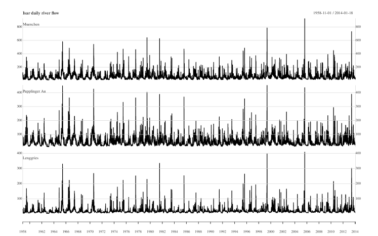
Figure 4: Daily river flow of the Isar river at three sites

To remove dependence between extremes over time, we decluster each series and retain only the cluster maxima based on three-day runs. Rounding of the measurements has no impact on parameter estimates and is henceforth neglected. The multivariate tail model outlined in Section 7 is next fitted to the cluster maxima. The thresholds $\boldsymbol{u}=(u_{1},u_{2},u_{3})$ were selected to be the 92% quantiles using the parameter stability plot of [42] (not shown here). Next, set $\boldsymbol{\theta}=(\boldsymbol{\eta},\boldsymbol{\xi},\boldsymbol{\alpha},\rho)$, where $\boldsymbol{\eta}$ and $\boldsymbol{\xi}$ are the marginal parameters of the generalized Pareto distribution in eq. 13 and $\rho$ and $\boldsymbol{\alpha}$ are the parameters of the scaled Dirichlet model. To estimate $\boldsymbol{\theta}$, the trivariate censored likelihood (14) could be used. To avoid numerical integration and because of the relative robustness to misspecification, we employed the pairwise composite log-likelihood $l_{C}$ of [28] instead; the loss of efficiency in this trivariate example is likely small. Specifically, we maximized

$$l_{C}(\boldsymbol{\theta})=\sum_{i=1}^{n}\sum_{j=1}^{d-1}\sum_{k=j+1}^{d}\left[\log g\{t_{j}(x_{ij}),t_{k}(x_{ik});\boldsymbol{\theta},t_{j}({u}_{j}),t_{k}(u_{k})\}+{\mathrm{I}}_{x_{ij}>u_{j}}\log J_{j}(x_{ij})+{\mathrm{I}}_{x_{ik}>u_{k}}\log J_{k}(x_{ik})\right],$$

where

$$g(y_{j},y_{k};\boldsymbol{\theta},u_{j},u_{k})=\begin{cases}\exp\{-\ell(1/u_{j},1/u_{k})\},&y_{j}\leq u_{j},y_{k}\leq u_{k}\\ -{\partial\ell(1/y_{j},1/u_{k})/\partial y_{j}}\exp\{-\ell(1/y_{j},1/u_{k})\},&y_{j}>u_{j},y_{k}\leq u_{k}\\ -{\partial\ell(1/u_{j},1/y_{k})}/{\partial y_{k}}\exp\{-\ell(1/u_{j},1/y_{k})\},&y_{j}\leq u_{j},y_{k}>u_{k}\\ \left[\left\{\partial\ell(1/y_{j},1/y_{k})/{\partial y_{j}}\right\}\left\{{\partial\ell(1/y_{j},1/y_{k})}/{\partial y_{k}}\right\}-dh^{\mathrm{D}}(y_{j},y_{k})\right]\exp\{-\ell(1/y_{j},1/y_{k})\},&y_{j}>u_{j},y_{k}>u_{k}\end{cases}$$

where $\ell=\ell^{\mathrm{D}}$ and for all $j=1,\dots,d$, $t_{j}$ and $J_{j}$ are as in Equation 15.

Uncertainty assessment can be done in the same way as for general estimating equations. Specifically, let $g(\boldsymbol{\theta})$ denote an unbiased estimating function and define the variability matrix $\mathbf{J}$, the sensitivity matrix $\mathbf{H}$ and the Godambe information matrix $\mathbf{G}$ as

$$\mathbf{J}={\mathrm{E}}\left(\frac{\partial g(\boldsymbol{\theta})}{\partial\boldsymbol{\theta}}\frac{\partial g(\boldsymbol{\theta})}{\partial\boldsymbol{\theta}}^{\top}\right),\qquad\mathbf{H}=-{\mathrm{E}}\left(\frac{\partial^{2}g(\boldsymbol{\theta})}{\partial\boldsymbol{\theta}\partial\boldsymbol{\theta}^{\top}}\right),\qquad\mathbf{G}=\mathbf{H}\mathbf{J}^{-1}\mathbf{H}.$$ (17)

The maximum composite likelihood estimator is strongly consistent and asymptotically normal, centered at the true parameter $\boldsymbol{\theta}$ with covariance matrix given by the inverse Godambe matrix $\mathbf{G}^{-1}$.

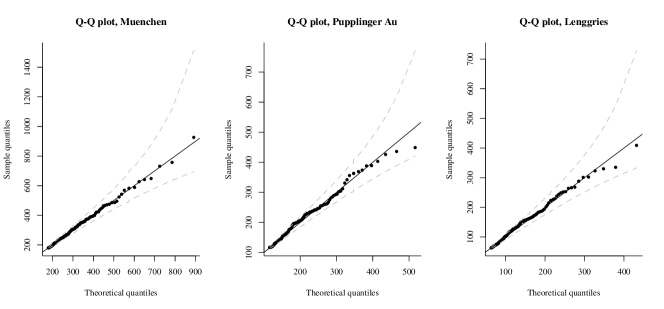
Figure 5: Marginal Q-Q plots for the three sites based on pairwise composite likelihood estimates for the scale and shape parameters obtained from the scaled Dirichlet model, retaining marginal exceedances of the 92% quantiles. The pointwise confidence intervals were obtained from the transformed Beta quantiles of the order statistics.

Using the pairwise composite log-likelihood $l_{C}$, we fitted the scaled extremal Dirichlet model as well as the logistic and negative logistic models that correspond to the negative and positive scaled extremal Dirichlet models, respectively, and the parameter restriction $\boldsymbol{\alpha}=\boldsymbol{1}_{d}$. The estimates of the marginal generalized Pareto parameters $\boldsymbol{\eta}$ and $\boldsymbol{\xi}$ are given in Table 1. As the estimates were obtained by maximizing $\ell_{C}$, their values depend on the fitted model; the line labeled “Marginal" corresponds to fitting the generalized Pareto distribution to threshold exceedances of each one of the three series separately. The marginal Q-Q plots displayed in Figure 5 indicate a good fit of the model as well.

	$\eta_{1}$	$\eta_{2}$	$\eta_{3}$	$\xi_{1}$	$\xi_{2}$	$\xi_{3}$
Scaled Dirichlet	123.2 (7.5)	84.4 (5)	68.1 (4.2)	0.05 (0.04)	-0.03 (0.04)	0.02 (0.04)
Neg. logistic	117.1 (6.8)	86.2 (5.1)	70 (4.3)	0.08 (0.04)	-0.05 (0.04)	0 (0.04)
Logistic	117.3 (6.8)	86.6 (5.1)	70.4 (4.3)	0.08 (0.04)	-0.05 (0.04)	0 (0.04)
ext. Dirichlet	114.4 (6.8)	84.3 (4.9)	68.2 (4.1)	0.12 (0.04)	-0.02 (0.04)	0.04 (0.04)
Marginal	129.1 (14.5)	95.1 (10.6)	76 (8.7)	-0.01 (0.08)	-0.15 (0.08)	-0.08 (0.08)

Table 1: Generalized Pareto parameter estimates and standard errors (in parenthesis) for the trivariate river example for four different models.

	$\alpha_{1}$	$\alpha_{2}$	$\alpha_{3}$	$\rho$
Scaled Dirichlet	0.76 (0.3)	1.65 (0.82)	2.03 (1.15)	$-$0.32 (0.1)
Neg. logistic	1	1	1	0.36 (0.02)
Logistic	1	1	1	0.28 (0.01)
ext. Dirichlet	3.34 (0.52)	10.2 (2.84)	12.78 (3.93)	1
Gradient score	1	2.72	2.66	$-$0.39

Table 2: Dependence parameters estimates and standard errors (in parenthesis) for the trivariate river example.

The estimates of the dependence parameters $\boldsymbol{\alpha}$ and $\rho$ are given in Table 2. The last line displays the maximum gradient score estimates were obtained from the raw data, i.e., ignoring the clustering, after transforming the observations to the standard Fréchet scale using the probability integral transform. We retained only the 10% largest values based on the $\ell_{p}$ norm with $p=20$; this risk functional is essentially a differentiable approximation of $\ell_{\infty}$. We selected the weight function $w(\boldsymbol{x},u)=\boldsymbol{x}[1-\exp\{-(\|\boldsymbol{x}\|_{p}/u-1)\}]$ based on [8] to reproduce approximate censoring. The estimates are similar to the composite maximum likelihood estimators, though not efficient.

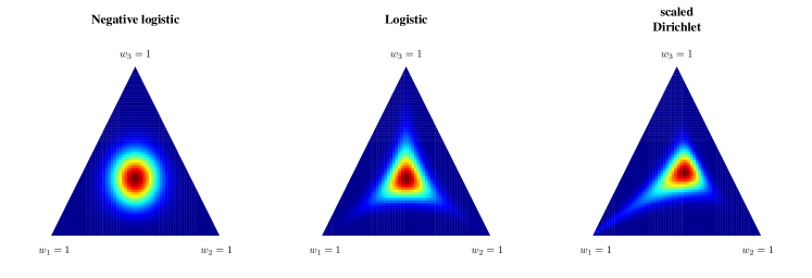
Figure 6: Angular density plots for the three models, the negative logistic (left), logistic (middle) and scaled Dirichlet (right). The colours correspond to log density values and range from red (high density) to blue (low density).

The angular densities of the fitted logistic, negative logistic and scaled extremal Dirichlet models are displayed in Figure 6. The right panel of this figure shows asymmetry caused by a few extreme events that only happened downstream. Whether this asymmetry is significant can be assessed through composite likelihood ratio tests; recall that the logistic model, the negative logistic model and the extremal Dirichlet model of [7] are all nested within the scaled extremal Dirichlet model. To this end, consider a partition of $\boldsymbol{\theta}=(\boldsymbol{\psi},\boldsymbol{\lambda})$ into a $q$ dimensional parameter of interest $\boldsymbol{\psi}$ and a $3d+1-q$ dimensional nuisance parameter $\boldsymbol{\lambda}$, and the corresponding partitions of the matrices $\mathbf{H}$, $\mathbf{J}$ and $\mathbf{G}$. Let $\widehat{\boldsymbol{\theta}}_{C}=(\widehat{\boldsymbol{\psi}}_{C},\widehat{\boldsymbol{\lambda}}_{C})$ denote the maximum composite likelihood parameter estimates and $\widehat{\boldsymbol{\theta}}_{0}=(\boldsymbol{\psi}_{0},\widehat{\boldsymbol{\lambda}}_{0})$ the restricted parameter estimates under the null hypothesis that the simpler model is adequate. The asymptotic distribution of the composite likelihood ratio test statistic $2\{\log l_{C}(\widehat{\boldsymbol{\theta}_{C}})-\log l_{C}(\widehat{\boldsymbol{\theta}_{0}})\}$ is equal to $\sum_{i=1}^{q}c_{i}Z_{i}$ where $Z_{i}$ are independent $\chi^{2}_{1}$ variables and $c_{i}$ are the eigenvalues of the $q\times q$ matrix $(\mathbf{H}_{\boldsymbol{\psi\psi}}-\mathbf{H}_{\boldsymbol{\psi\lambda}}\mathbf{H}^{-1}_{\boldsymbol{\lambda\lambda}}\mathbf{H}_{\boldsymbol{\lambda\psi}})\mathbf{G}^{-1}_{\boldsymbol{\psi\psi}}$; see [26]. We estimated the inverse Godambe information matrix, $\smash{\mathbf{G}^{-1}}$, by the empirical covariance of ${B}$ nonparametric bootstrap replicates. The sensitivity matrix $\mathbf{H}$ was obtained from the Hessian matrix at the maximum composite likelihood estimate and the variability matrix $\mathbf{J}$ from eq. 17. Since the Coles–Tawn extremal Dirichlet, negative logistic and logistic models are nested within the scaled Dirichlet family, we test for a restriction to these simpler models; the respective approximate $P$-values were 0.003, 0.74 and 0.78. These values suggest that while the Coles–Tawn extremal Dirichlet model is clearly not suitable, there is not sufficient evidence to discard the logistic and negative logistic models. The effects of possible model misspecification are also visible for the Coles–Tawn extremal Dirichlet model, as the parameter values of $\alpha_{1},\alpha_{2}$ and $\alpha_{3}$ are very large (viz. Table 2) and this induces negative bias in the shape parameter estimates, as can be seen from Table 1.

Appendix 9. : Discussion

In this article, we have identified extremal attractors of copulas and survival copulas of Liouville random vectors $R\boldsymbol{D}_{\boldsymbol{\alpha}}$, where $\boldsymbol{D}_{\boldsymbol{\alpha}}$ has a Dirichlet distribution on the unit simplex with parameters $\boldsymbol{\alpha}$, and $R$ is a strictly positive random variable independent of $\boldsymbol{D}_{\boldsymbol{\alpha}}$. The limiting stable tail dependence functions can be embedded in a single family, which can capture asymmetry and provides a valid model in dimension $d$. The latter is novel and termed here the scaled extremal Dirichlet; it includes the well-known logistic, negative logistic as well as the Coles–Tawn extremal Dirichlet models as special cases. In particular, therefore, this paper is first to provide an example of a random vector attracted to the Coles–Tawn extremal Dirichlet model, which was derived by enforcing moment constraints on a simplex distribution rather than as the limiting distribution of a random vector.

A scaled extremal Dirichlet stable tail dependence function $\ell^{\mathrm{D}}$ has $d+1$ parameters, $\rho$ and $\boldsymbol{\alpha}$. The parameter vector $\boldsymbol{\alpha}$ is inherited from $\boldsymbol{D}_{\boldsymbol{\alpha}}$ and induces asymmetry in $\ell^{\mathrm{D}}$. The parameter $\rho$ comes from the regular variation of $R$ at zero and infinity, respectively; this is reminiscent of the extremal attractors of elliptical distributions [33]. The magnitude of $\rho$ has impact on the strength of dependence while its sign changes the overall shape of $\ell^{\mathrm{D}}$. Having $d+1$ parameters, the scaled extremal Dirichlet model may not be sufficiently rich to account for spatial dependence, unlike the Hüsler–Reiss or the extremal Student-$t$ models, which have one parameter for each pair of variables and are thus easily combined with distances. Also, it is less flexible than Dirichlet mixtures [4], which are however hard to estimate in high dimensions and require sophisticated machinery. To achieve greater flexibility, the scaled extremal Dirichlet model could perhaps be extended by working with more general scale mixtures, such as of the weighted Dirichlet distributions considered, e.g., in [18].

Nonetheless, the scaled extremal Dirichlet model may naturally find applications whenever asymmetric extremal dependence is suspected; the latter may be caused, e.g., by causal relationships between the variables [15]. The stochastic structure of the scaled extremal Dirichlet model has several major advantages, that make the model easy to interpret, estimate and simulate from. Its angular density has a simple form; in contrast to the asymmetric generalizations of the logistic and negative logistic models, this model does not place any mass on the vertices and lower-dimensional facets of the unit simplex. Another plus is the tractability of the de Haan representation and of the extremal functions, both expressible in terms of independent scaled Gamma variables; this allows for feasible inference and stochastic simulation. While the scaled extremal Dirichlet stable tail dependence function $\ell^{\mathrm{D}}$ does not have a closed form in general, closed-form algebraic expressions exist when $\boldsymbol{\alpha}$ is integer-valued and in the bivariate case. Model selection for well-known families of extreme-value distributions can be performed through likelihood ratio tests. Another potentially useful feature is that $\rho\in(-\infty,\infty)$ can be allowed, with the convention that all variables whose indices $i$ are such that $-\rho\leq-\alpha_{i}$ are independent.

Acknowledgment

Funding in partial support of this work was provided by the Natural Sciences and Engineering Research Council (RGPIN-2015-06801, CGSD3-459751-2014), the Canadian Statistical Sciences Institute, and the Fonds de recherche du Québec – Nature et technologies (2015–PR–183236). We thank the acting Editor-in-Chief, Richard Lockhart, the Associate Editor and two anonymous referees for their valuable suggestions.

Appendix A Proofs from Section 2

Proof of Proposition 2. To prove parts (a) and (b), recall that $1/X_{i}$ is distributed as $1/(RD_{i})$, where $D_{i}\sim\mathsf{Beta}(\alpha_{i},\bar{\alpha}-\alpha_{i})$ is independent of $R$. Furthermore, it is easy to show that $1/D_{i}\in\mathcal{M}(\Phi_{\alpha_{i}})$, which implies that $\mathrm{E}(1/D_{i}^{\beta})<\infty$ for any $\beta<\alpha_{i}$. The extremal behavior of $1/X_{i}$ will thus be determined by the extremal behavior of either $1/R$ or $1/D_{i}$, depending on which one has a heavier tail. Indeed, Breiman’s Lemma [5] implies that $1/X_{i}\in\mathcal{M}(\Phi_{\rho})$ if $1/R\in\mathcal{M}(\Phi_{\rho})$ for some $\rho<\alpha_{i}$ and that $1/X_{i}\in\mathcal{M}(\Phi_{\alpha_{i}})$ if $\mathrm{E}(1/R^{\alpha_{i}+\varepsilon})<\infty$ for some $\varepsilon>0$. Finally, the fact that $1/X_{i}\in\mathcal{M}(\Phi_{\alpha_{i}})$ when $1/R\in\mathcal{M}(\Phi_{\alpha_{i}})$ follows directly from the Corollary to Theorem 3 in [11].

The following lemma is a side result of Proposition 2, which is needed in the subsequent proofs.

Lemma 1.

Suppose that $\boldsymbol{X}=R\boldsymbol{D}_{\alpha}$. If $1/R\in\mathcal{M}(\Phi_{\alpha_{i}})$ for some $i\in\{1,\dots,d\}$, then

$$\lim_{x\to\infty}\frac{\Pr\left({1}/{R}>x\right)}{\Pr\left({1}/{X_{i}}>x\right)}=0.$$

Proof of Lemma 1.

Because $1/R\in\mathcal{M}(\Phi_{\alpha_{i}})$, $\Pr(1/R>x)$ is regularly varying with index $-\alpha_{i}$. In particular, for any $b\in(0,1)$, $\Pr(1/R>xb)/\Pr(1/R>x)\to b^{-\alpha_{i}}$ as $x\to\infty$. An application of Fatou’s lemma thus gives

$$\liminf_{x\to\infty}\frac{\Pr(1/X_{i}>x)}{\Pr(1/R>x)} =\liminf_{x\to\infty}\int_{0}^{1}\frac{\Pr(1/R>xb)}{\Pr(1/R>x)}f_{D_{i}}(b){\,\textrm{d}}b\geq\int_{0}^{1}\frac{b^{-1}(1-b)^{\bar{\alpha}-\alpha_{i}-1}}{\textrm{B}(\alpha_{i},\bar{\alpha}-\alpha_{i})}{\,\textrm{d}}b=\infty$$

and hence the result.

Appendix B Proofs from Section 3

First recall the following property of the Dirichlet distribution, which is easily shown using the transformation formula for Lebesgue densities.

Lemma 2.

Let $\boldsymbol{D}_{\alpha}$ be a Dirichlet random vector with parameters $\boldsymbol{\alpha}$. Then for any $2\leq k\leq d$ and any collection of distinct indices $1\leq i_{1}<\dots<i_{k}\leq d$,

$$(D_{i_{1}},\dots,D_{i_{k}})\stackrel{{\scriptstyle\mbox{\tiny d}}}{{=}}B_{i_{1},\dots,i_{k}}\times\boldsymbol{D}_{(\alpha_{i_{1}},\dots,\alpha_{i_{k}})},$$

where $B_{i_{1},\dots,i_{k}}\sim\mathsf{Beta}(\alpha_{i_{1}}+\cdots+\alpha_{i_{k}},\bar{\alpha}-(\alpha_{i_{1}}+\cdots+\alpha_{i_{k}}))$ is independent of the $k$-variate Dirichlet vector $\boldsymbol{D}_{(\alpha_{i_{1}},\dots,\alpha_{i_{k}})}$ with parameters $(\alpha_{i_{1}},\dots,\alpha_{i_{k}})$.

Proof of Theorem 1. In order to prove part (a), recall that $\|\boldsymbol{X}\|\stackrel{{\scriptstyle\mbox{\tiny d}}}{{=}}R$ is independent of $\boldsymbol{X}/\|\boldsymbol{X}\|\stackrel{{\scriptstyle\mbox{\tiny d}}}{{=}}\boldsymbol{D}_{\boldsymbol{\alpha}}$. Because $R\in\mathcal{M}(\Phi_{\rho})$, there exists a sequence $(b_{n})$ of constants in $(0,\infty)$ such that, for any Borel set $B\subseteq\mathbb{S}_{d}$ and any $r>0$,

$$\lim_{n\to\infty}n\Pr\left(\|\boldsymbol{X}\|>b_{n}r,\frac{\boldsymbol{X}}{\|\boldsymbol{X}\|}\in B\right)=\lim_{n\to\infty}n\Pr(R>b_{n}r)\Pr(\boldsymbol{D}_{\boldsymbol{\alpha}}\in B)=r^{-\rho}\Pr(\boldsymbol{D}_{\boldsymbol{\alpha}}\in B).$$

By Corollary 5.18 in [35], $\boldsymbol{X}\in\mathcal{M}(H_{0})$ where for all $\boldsymbol{x}\in\mathbb{R}_{+}^{d}$,

$$H_{0}(\boldsymbol{x})=\exp\left[-\mathrm{E}\left\{\max\left(\frac{D_{1}^{\rho}}{x_{1}^{\rho}},\dots,\frac{D_{d}^{\rho}}{x_{d}^{\rho}}\right)\right\}\right].$$

Let $\mathrm{B}(\cdot,\cdot)$ denote the Beta function. The univariate margins of $H_{0}$ are given, for all $i=1,\dots,d$ and $x>0$, by

$$F_{0i}(x) =\exp\left\{-x^{-\rho}\mathrm{E}(D_{i}^{\rho})\right\}=\exp\left\{-x^{-\rho}\frac{\mathrm{B}(\rho+\alpha_{i},\bar{\alpha}-\alpha_{i})}{\mathrm{B}(\alpha_{i},\bar{\alpha}-\alpha_{i})}\right\}=\exp\left\{-x^{-\rho}\frac{\Gamma(\alpha_{i}+\rho)\Gamma(\bar{\alpha})}{\Gamma(\bar{\alpha}+\rho)\Gamma(\alpha_{i})}\right\}$$

for $i\in\{1,\ldots,d\}$. The copula of $H_{0}$ then satisfies, for all $\boldsymbol{u}\in[0,1]^{d}$,

$$C_{0}(\boldsymbol{u})=H_{0}\{F_{01}^{-1}(u_{1}),\dots,F_{0d}^{-1}(u_{d})\}=\exp\left(-\frac{\Gamma(\bar{\alpha}+\rho)}{\Gamma(\bar{\alpha})}\mathrm{E}\left[\max_{1\leq i\leq d}\left\{\frac{(-\log u_{i})\Gamma(\alpha_{i})D_{i}^{\rho}}{\Gamma(\alpha_{i}+\rho)}\right\}\right]\right).$$

By Equation 2, the stable tail dependence function of $C_{0}$ thus indeed equals, for all $\boldsymbol{x}\in\mathbb{R}_{+}^{d}$,

$$\ell(\boldsymbol{x})=\frac{\Gamma(\bar{\alpha}+\rho)}{\Gamma(\bar{\alpha})}\mathrm{E}\left[\max\left\{\frac{x_{1}\Gamma(\alpha_{1})D_{1}^{\rho}}{\Gamma(\alpha_{1}+\rho)},\dots,\frac{x_{d}\Gamma(\alpha_{d})D_{d}^{\rho}}{\Gamma(\alpha_{d}+\rho)}\right\}\right].$$

The part (b) follows directly from Proposition 2.2 in [19] upon setting $p=1$ and taking, for $i=1,\dots,d$ and $j=1,\dots,d$, $\lambda_{ij}=1$ whenever $i=j$ and $\lambda_{ij}=0$ otherwise.

To prove part (c), recall first that from Proposition 1, for $i=1,\dots,d$, $X_{i}\in\mathcal{M}(\Psi_{\rho+\bar{\alpha}-\alpha_{i}})$ and hence there exist sequences $(a_{ni})\in(0,\infty)$, $(b_{ni})\in\mathbb{R}$, such that for all $x\in\mathbb{R}$,

$$\lim_{n\to\infty}n\Pr(X_{i}>a_{ni}x+b_{ni})=-\log\{\Psi_{\rho+\bar{\alpha}-\alpha_{i}}(x)\}.$$

Next, observe that as in the proof of Proposition 5.27 in [35], $\boldsymbol{X}\in\mathcal{M}(H_{0})$ follows if for all $1\leq i<j\leq d$ and $x_{k}$ such that $\Psi_{\rho+\bar{\alpha}-\alpha_{k}}(x_{k})>0$ for $k=i,j$,

$$\lim_{n\to\infty}n\Pr(X_{i}>a_{ni}x_{i}+b_{ni},X_{j}>a_{nj}x_{j}+b_{nj})=0.$$ (B.1)

To prove that (B.1) indeed holds, it suffices to assume that $d=2$. This is because for arbitrary indices $1\leq i<j\leq d$, Lemma 2 implies that $(X_{i},X_{j})\stackrel{{\scriptstyle\mbox{\tiny d}}}{{=}}R^{*}(B,1-B)$, where $B\sim\mathrm{Beta}(\alpha_{i},\alpha_{j})$, $R^{*}\stackrel{{\scriptstyle\mbox{\tiny d}}}{{=}}RY$ is independent of $B$ and $Y\sim\mathrm{Beta}(\alpha_{i}+\alpha_{j},\bar{\alpha}-\alpha_{i}-\alpha_{j})$ is independent of $B$ and $R$. Because $\Pr(R^{*}\leq 0)=0$, Theorem 4.5 in [20] implies that $R^{*}\in\mathcal{M}(\Psi_{\rho+\bar{\alpha}-\alpha_{i}-\alpha_{j}})$ when $R\in\mathcal{M}(\Psi_{\rho})$ for some $\rho>0$. Thus suppose that $d=2$ and write $(D_{1},D_{2})\equiv(B,1-B)$, where $B\sim\mathsf{Beta}(\alpha_{1},\alpha_{2})$. Fix arbitrary $x_{1},x_{2}\in\mathbb{R}$ are such that $\Psi_{\rho+\bar{\alpha}-\alpha_{i}}(x_{i})>0$ for $i=1,2$. Then because for any $a,c>0$ and $b\in(0,1)$, $\max\{a/b,c/(1-b)\}\geq a+c$, one has

$$0\leq\Pr(X_{1}>a_{n1}x_{1}+b_{n1},X_{2}>a_{n2}x_{2}+b_{n2}) =\Pr\left\{R>\max\left(\frac{a_{n1}x_{1}+b_{n1}}{B},\frac{a_{n2}x_{2}+b_{n2}}{1-B}\right)\right\}$$

$$\leq\Pr(R>a_{n1}x_{1}+b_{n1}+a_{n2}x_{2}+b_{n2}).$$

In order to prove Equation B.1, it thus suffices to show that

$$\lim_{n\to\infty}n\Pr(R>a_{n1}x_{1}+b_{n1}+a_{n2}x_{2}+b_{n2})=0.$$ (B.2)

This however follows immediately from the fact that if $R\in\mathcal{M}(\Psi_{\rho})$ for some $\rho>0$, the upper end-point $r$ of $R$, viz. $r=\sup\{x:\Pr(R\leq x)<1\}$, is finite. Because for $i=1,2,$ $r$ is also the upper endpoint of $X_{i}$, $a_{ni}x_{i}+b_{ni}\to r$ as $n\to\infty$. This means that there exists $n_{0}\in\mathbb{N}$ so that for all $n\geq n_{0}$, $a_{n1}x_{1}+b_{n1}+a_{n2}x_{2}+b_{n2}>r$ and $\Pr(R>a_{n1}x_{1}+b_{n1}+a_{n2}x_{2}+b_{n2})=0$. This proves Equation B.1 and hence also Theorem 1 (c). Note that alternatively, part (c) could be proved using Theorem 2.1 in [19] similarly to the proof of Proposition 2.2 therein.

The proof of Theorem 2 requires the following technical lemma.

Lemma 3.

Suppose that $\boldsymbol{D}_{\boldsymbol{\alpha}}=(D_{1},\dots,D_{d})$ is a Dirichlet random vector with parameters $\boldsymbol{\alpha}$. Further let $R$ be a positive random variable independent of $\boldsymbol{D}_{\boldsymbol{\alpha}}$ such that $\Pr(R\leq 0)=0$, and let $\boldsymbol{X}=R\boldsymbol{D}_{\alpha}$. Then for any $1\leq i<j\leq d$ and any $x_{i},x_{j}\in(0,\infty)$,

$$\lim_{n\to\infty}n\Pr\left(\frac{1}{X_{i}}>a_{ni}x_{i},\frac{1}{X_{j}}>a_{nj}x_{j}\right)=0$$

if either:

1. $1/R\in\mathcal{M}(\Phi_{\rho})$ with $\rho\in[\alpha_{i}\wedge\alpha_{j},\alpha_{1}\vee\alpha_{2}]$, and for $k=i,j$, $(a_{nk})$ is a sequence of positive constants such that $n\Pr(1/X_{k}>a_{nk}x_{k})\to x_{k}^{-(\alpha_{k}\wedge\rho)}$ as $n\to\infty$;

2. $\textrm{E}(1/R^{\beta})<\infty$ for some $\beta>\alpha_{i}\vee\alpha_{j}$ and for $k=i,j$, $(a_{nk})$ is a sequence of positive constants such that $n\Pr(1/X_{k}>a_{nk}x_{k})\to x_{k}^{-\alpha_{k}}$ as $n\to\infty$.

Proof of Lemma 3. Observe first that when $d>2$, Lemma 2 implies that $(X_{i},X_{j})\stackrel{{\scriptstyle\mbox{\tiny d}}}{{=}}R^{*}(B,1-B)$, where $R^{*}\mathchoice{\mathrel{\hbox to0.0pt{$\displaystyle\perp$\hss}\mkern 2.0mu{\displaystyle\perp}}}{\mathrel{\hbox to0.0pt{$\textstyle\perp$\hss}\mkern 2.0mu{\textstyle\perp}}}{\mathrel{\hbox to0.0pt{$\scriptstyle\perp$\hss}\mkern 2.0mu{\scriptstyle\perp}}}{\mathrel{\hbox to0.0pt{$\scriptscriptstyle\perp$\hss}\mkern 2.0mu{\scriptscriptstyle\perp}}}B$, $B\sim\mathsf{Beta}(\alpha_{i},\alpha_{j})$ and $R^{*}=RY$, with $Y\mathchoice{\mathrel{\hbox to0.0pt{$\displaystyle\perp$\hss}\mkern 2.0mu{\displaystyle\perp}}}{\mathrel{\hbox to0.0pt{$\textstyle\perp$\hss}\mkern 2.0mu{\textstyle\perp}}}{\mathrel{\hbox to0.0pt{$\scriptstyle\perp$\hss}\mkern 2.0mu{\scriptstyle\perp}}}{\mathrel{\hbox to0.0pt{$\scriptscriptstyle\perp$\hss}\mkern 2.0mu{\scriptscriptstyle\perp}}}R$ and $Y\sim\mathsf{Beta}(\alpha_{i}+\alpha_{j},\bar{\alpha}-\alpha_{i}-\alpha_{j})$. Now note that $1/Y\in\mathcal{M}(\Phi_{\alpha_{i}+\alpha_{j}})$. Thus if $1/R\in\mathcal{M}(\Phi_{\rho})$ for $\rho\in[\alpha_{i}\wedge\alpha_{j},\alpha_{1}\vee\alpha_{2}]$, $\rho<\alpha_{i}+\alpha_{j}$ and Breiman’s Lemma implies that $1/R^{*}\in\mathcal{M}(\Phi_{\rho})$. Further, if $\textrm{E}(1/R^{\beta})<\infty$ for some $\beta\in(\alpha_{i}\vee\alpha_{j},\alpha_{i}+\alpha_{j})$, $\textrm{E}\{1/(R^{*})^{\beta}\}<\infty$ given that $\textrm{E}(1/Y^{\beta})<\infty$. We can thus assume without loss of generality that $d=2$ and $\alpha_{1}\leq\alpha_{2}$; we shall also write $(D_{1},D_{2})\equiv(B,1-B)$, where $B\sim\mathsf{Beta}(\alpha_{1},\alpha_{2})$.

To prove part (i), note first that the existence of the sequences $(a_{nk})$, $k=i,j$, follows from Proposition 2, by which $1/X_{k}\in\mathcal{M}(\Phi_{\rho\wedge\alpha_{k}})$ for $k=i,j$, and the Poisson approximation [12, Proposition 3.1.1]. Next, observe that for any constants $a,c>0$ and any $b\in(0,1)$,

$$\frac{ac}{a+c}\leq ab\vee c(1-b)<a\vee c.$$ (B.3)

Indeed, when $b<c/(a+c)$, $ab\vee c(1-b)=c(1-b)$ and $c(1-b)\in(ac/(a+c),c)$, while when $b\geq c/(a+c)$, $ab\vee c(1-b)=ab$ and $ab\in[ac/(a+c),a)$. To show the claim in part (i), distinguish the cases below:

Case I. $\alpha_{1}=\alpha_{2}$. Here, $\rho=\alpha_{1}=\alpha_{2}$ and $X_{1}\stackrel{{\scriptstyle\mbox{\tiny d}}}{{=}}X_{2}$, so that $a_{n1}/a_{n2}\to 1$ by the Convergence to Types Theorem [35]. By Equation B.3,

$$0\leq n\Pr\left(\frac{1}{X_{1}}>a_{n1}x_{1},\frac{1}{X_{2}}>a_{n2}x_{2}\right)=n\Pr\left[\frac{1}{R}>\max\{a_{n1}x_{1}B,a_{n2}x_{2}(1-B)\}\right]\leq n\Pr\left(\frac{1}{R}>\frac{a_{n1}a_{n2}x_{1}x_{2}}{a_{n1}x_{1}+a_{n2}x_{2}}\right).$$ (B.4)

Because $(x_{1}x_{2})/\{(a_{n1}/a_{n2})x_{1}+x_{2}\}\to(x_{1}x_{2})/(x_{1}+x_{2})$ as $n\to\infty$,

$$\lim_{n\to\infty}n\Pr\left(\frac{1}{X_{1}}>\frac{a_{n1}a_{n2}x_{1}x_{2}}{a_{n1}x_{1}+a_{n2}x_{2}}\right)=\left(\frac{x_{1}x_{2}}{x_{1}+x_{2}}\right)^{-\alpha_{1}}.$$

Furthermore, by Lemma 1, given that $(a_{n1}a_{n2}x_{1}x_{2})/(a_{n1}x_{1}+a_{n2}x_{2})\to\infty$ as $n\to\infty$,

$$\lim_{n\to\infty}\dfrac{\Pr\left({1}/{R}>\frac{a_{n1}a_{n2}x_{1}x_{2}}{a_{n1}x_{1}+a_{n2}x_{2}}\right)}{\Pr\left({1}/{X_{1}}>\frac{a_{n1}a_{n2}x_{1}x_{2}}{a_{n1}x_{1}+a_{n2}x_{2}}\right)}=0,$$

so that the right-hand side in Equation B.4 tends to $0$ as $n\to\infty$, and this implies the claim.

Case II. $\alpha_{1}<\alpha_{2}$ and $\rho=\alpha_{2}$. Then for $i=1,2$, there exists a slowly varying function $L_{i}$ such that $a_{ni}=n^{1/\alpha_{i}}L_{i}(n)$. Hence $a_{n2}/a_{n1}\to 0$ and $(x_{1}x_{2})/\{x_{1}+x_{2}(a_{n2}/a_{n1})\}\to x_{2}$ as $n\to\infty$. Consequently,

$$\lim_{n\to\infty}n\Pr\left(\frac{1}{X_{2}}>\frac{a_{n1}a_{n2}x_{1}x_{2}}{a_{n1}x_{1}+a_{n2}x_{2}}\right)=x_{2}^{-\alpha_{2}}.$$

Moreover, by Lemma 1, given that $(a_{n1}a_{n2}x_{1}x_{2})/(a_{n1}x_{1}+a_{n2}x_{2})\to\infty$ as $n\to\infty$,

$$\lim_{n\to\infty}\dfrac{\Pr\left(1/R>\frac{a_{n1}a_{n2}x_{1}x_{2}}{a_{n1}x_{1}+a_{n2}x_{2}}\right)}{\Pr\left(1/{X_{2}}>\frac{a_{n1}a_{n2}x_{1}x_{2}}{a_{n1}x_{1}+a_{n2}x_{2}}\right)}=0,$$

so that again the right-hand side in Equation B.4 tends to $0$ as $n\to\infty$.

Case III. $\alpha_{1}<\alpha_{2}$ and $\rho\in[\alpha_{1},\alpha_{2})$. In this case, $1/X_{1}\in\mathcal{M}(\Phi_{\alpha_{1}})$ and $1/X_{2}\in\mathcal{M}(\Phi_{\rho})$. Therefore, either directly when $\rho>\alpha_{1}$ or by Lemma 1, one can easily deduce that

$$\lim_{x\to\infty}\frac{\Pr(1/R>x)}{\Pr(1/X_{1}>x)}=0.$$ (B.5)

At the same time, Breiman’s Lemma [5] implies that

$$\lim_{x\to\infty}\frac{\Pr(1/R>x)}{\Pr(1/X_{2}>x)}=\frac{1}{\mathrm{E}\{1/(1-B)^{\rho}\}}=\frac{\mathrm{B}(\alpha_{1},\alpha_{2})}{\mathrm{B}(\alpha_{1},\alpha_{2}-\rho)}.$$ (B.6)

Hence, for any $b\in(0,1)$, the limit of $n\Pr\left\{1/R>a_{n2}x_{2}(1-b)\right\}$ as $n\to\infty$ equals

$$\lim_{n\to\infty}n\Pr\left\{1/X_{2}>a_{n2}x_{2}(1-b)\right\}\frac{\Pr\left\{1/R>a_{n2}x_{2}(1-b)\right\}}{\Pr\left\{1/X_{2}>a_{n2}x_{2}(1-b)\right\}}=\{x_{2}(1-b)\}^{-\rho}\frac{\mathrm{B}(\alpha_{1},\alpha_{2})}{\mathrm{B}(\alpha_{1},\alpha_{2}-\rho)}$$

so that

$$\lim_{n\to\infty}\int_{0}^{1}n\Pr\{1/R>a_{n2}x_{2}(1-b)\}\frac{b^{\alpha_{1}-1}(1-b)^{\alpha_{2}-1}}{\textrm{ B}(\alpha_{1},\alpha_{2})}{\,\textrm{d}}b=n\Pr(1/X_{2}>a_{n2}x_{2})=x_{2}^{-\rho}\\ =x_{2}^{-\rho}\int_{0}^{1}\frac{b^{\alpha_{1}-1}(1-b)^{\alpha_{2}-\rho-1}}{\textrm{ B}(\alpha_{1},\alpha_{2}-\rho)}{\,\textrm{d}}b=\int_{0}^{1}\lim_{n\to\infty}n\Pr\{1/R>a_{n2}x_{2}(1-b)\}\frac{b^{\alpha_{1}-1}(1-b)^{\alpha_{2}-1}}{\textrm{B}(\alpha_{1},\alpha_{2})}{\,\textrm{d}}b.$$ (18)

Given that for any $b\in(0,1)$, $\Pr\{1/R>a_{n1}x_{1}b,1/R>a_{n2}x_{2}(1-b)\}\leq\Pr\{1/R>a_{n2}x_{2}(1-b)\}$,

$$\int_{0}^{1}\liminf_{n\to\infty}\bigl{(}n\bigl{[}\Pr\{1/R>a_{n2}x_{2}(1-b)\}-\Pr\{1/R>a_{n1}x_{1}b,1/R>a_{n2}x_{2}(1-b)\}\bigr{]}\bigr{)}\frac{b^{\alpha_{1}-1}(1-b)^{\alpha_{2}-1}}{\textrm{B}(\alpha_{1},\alpha_{2})}{\,\textrm{d}}b$$

$$\leq\liminf_{n\to\infty}\int_{0}^{1}n\bigl{[}\Pr\{1/R>a_{n2}x_{2}(1-b)\}-\Pr\{1/R>a_{n1}x_{1}b,1/R>a_{n2}x_{2}(1-b)\}\bigr{]}\frac{b^{\alpha_{1}-1}(1-b)^{\alpha_{2}-1}}{\textrm{B}(\alpha_{1},\alpha_{2})}{\,\textrm{d}}b$$

by Fatou’s Lemma. Because of Equation 18, this inequality simplifies to

$$x_{2}^{-\rho}-\int_{0}^{1}\limsup_{n\to\infty}\bigl{[}n\Pr\{1/R>a_{n1}x_{1}b,1/R>a_{n2}x_{2}(1-b)\}\bigr{]}\frac{b^{\alpha_{1}-1}(1-b)^{\alpha_{2}-1}}{\textrm{B}(\alpha_{1},\alpha_{2})}{\,\textrm{d}}b$$

$$\leq x_{2}^{-\rho}-\limsup_{n\to\infty}\int_{0}^{1}n\Pr\{1/R>a_{n1}x_{1}b,1/R>a_{n2}x_{2}(1-b)\}\frac{b^{\alpha_{1}-1}(1-b)^{\alpha_{2}-1}}{\textrm{B}(\alpha_{1},\alpha_{2})}{\,\textrm{d}}b$$

and hence

$$0\leq\limsup_{n\to\infty}\bigl{\{}n\Pr(1/X_{1}>a_{n1}x_{1},1/X_{2}>a_{n2}x_{2})\bigr{\}}\\ \leq\int_{0}^{1}\limsup_{n\to\infty}\bigl{[}n\Pr\{1/R>a_{n1}x_{1}b,1/R>a_{n2}x_{2}(1-b)\}\bigr{]}\frac{b^{\alpha_{1}-1}(1-b)^{\alpha_{2}-1}}{\textrm{ B}(\alpha_{1},\alpha_{2})}{\,\textrm{d}}b.$$

To show the desired claim, it thus suffices to show that for arbitrary $b\in(0,1)$,

$$\lim_{n\to\infty}n\Pr\{1/R>a_{n1}x_{1}b,1/R>a_{n2}x_{2}(1-b)\}=0.$$ (B.8)

To this end, fix $b\in(0,1)$ and observe that $a_{n1}/a_{n2}\to\infty$. Indeed, if $\rho>\alpha_{1}$, this follows directly from the fact that $a_{n1}=n^{1/\alpha_{1}}L_{1}(n)$ and $a_{n2}=n^{1/\rho}L_{2}(n)$ for some slowly varying functions $L_{1},L_{2}$. When $\rho=\alpha_{1}$, suppose that $\liminf_{n\to\infty}a_{n1}/a_{n2}$ were finite. Then there exists a subsequence $a_{n_{k}1}/a_{n_{k}2}$ such that $a_{n_{k}1}/a_{n_{k}2}\to a$ as $k\to\infty$ for some $a\in[0,\infty)$. Hence, for a fixed $\varepsilon>0$ and all $k\geq k_{0}$, $a_{n_{k}1}/a_{n_{k}2}\leq a+\varepsilon$. Using the latter observation and Equation B.6,

$$\lim_{k\to\infty}n_{k}\Pr(1/R>a_{n_{k}1})\geq\lim_{k\to\infty}n_{k}\Pr\{1/R>a_{n_{k}2}(a+\varepsilon)\}\\ =\lim_{k\to\infty}n_{k}\Pr\{1/X_{2}>a_{n_{k}2}(a+\varepsilon)\}\frac{\Pr\{1/R>a_{n_{k}2}(a+\varepsilon)\}}{\Pr\{1/X_{2}>a_{n_{k}2}(a+\varepsilon)\}}=(a+\varepsilon)^{-\rho}\frac{\mathrm{B}(\alpha_{1},\alpha_{2})}{\mathrm{B}(\alpha_{1},\alpha_{2}-\rho)}>0.$$

At the same time, by Equation B.5,

$$\lim_{k\to\infty}n_{k}\Pr(1/R>a_{n_{k}1})=\lim_{k\to\infty}n_{k}\Pr(1/X_{1}>a_{n_{k}1})\frac{\Pr(1/R>a_{n_{k}1})}{\Pr(1/X_{1}>a_{n_{k}1})}=0$$

and hence a contradiction. Therefore, $\liminf_{n\to\infty}a_{n1}/a_{n2}=\infty$ and hence $a_{n1}/a_{n2}\to\infty$ as $n\to\infty$. Because $a_{n1}b>a_{n2}(1-b)$ if and only if $b>a_{n2}/(a_{n1}+a_{n2})$ and $a_{n2}/(a_{n1}+a_{n2})\to 0$ as $n\to\infty$, there exists $n_{0}$ such that for all $n\geq n_{0}$,

$$n\Pr\{1/R>a_{n1}x_{1}b,1/R>a_{n2}x_{2}(1-b)\}=n\Pr(1/R>a_{n1}x_{1}b)=n\Pr(1/X_{1}>a_{n1}x_{1}b)\frac{\Pr(1/R>a_{n1}x_{1}b)}{\Pr(1/X_{1}>a_{n1}x_{1}b)}.$$

The last expression tends to $0$ as $n\to\infty$ by Equation B.5 and hence Equation B.8 indeed holds.

To prove part (ii), first recall that by Proposition 2 (b), $1/X_{i}\in\mathcal{M}(\Phi_{\alpha_{i}})$, $i=1,2$, and hence the scaling sequences $(a_{n1})$ and $(a_{n2})$ indeed exist. Recall that for $i=1,2$, $a_{ni}=n^{1/\alpha_{i}}L_{i}(n)$ for some slowly varying function $L_{i}$. As in the proof of part (i), $n\Pr(1/X_{1}>a_{n1}x_{1},1/X_{2}>a_{n2}x_{2})$ can be bounded above by the right-hand side in Equation B.4. Markov’s inequality further implies that for $\beta\in(\alpha_{2},\alpha_{1}+\alpha_{2})$ such that $\textrm{E}(1/R^{\beta})<\infty$,

$$n\Pr\left(\frac{1}{R}>\frac{a_{n1}a_{n2}x_{1}x_{2}}{a_{n1}x_{1}+a_{n2}x_{2}}\right) \leq n{\mathrm{E}}\left(1/R^{\beta}\right)\frac{(a_{n1}x_{1}+a_{n2}x_{2})^{\beta}}{(a_{n1}a_{n2}x_{1}x_{2})^{\beta}}=\frac{{\mathrm{E}}\left(1/R^{\beta}\right)}{(x_{1}x_{2})^{\beta}}\left\{\frac{x_{1}}{n^{1/\alpha_{2}-1/\beta}L_{2}(n)}+\frac{x_{2}}{n^{1/\alpha_{1}-1/\beta}L_{1}(n)}\right\}^{\beta}$$

The right-most expression tends to $0$ as $n\to\infty$ because for any $i=1,2$ and $\rho>0$, $n^{\rho}L_{i}(n)\to\infty$.

Proof of Theorem 2. First note that a positive random vector $\boldsymbol{Y}$ is in the maximum domain of attraction of a multivariate extreme-value distribution $H_{0}$ with Fréchet margins if and only if there exist sequences of positive constants $(a_{ni})\in(0,\infty)$, $i=1,\dots,d$, so that, for all $\boldsymbol{y}\in\mathbb{R}_{+}^{d}$,

$$\lim_{n\to\infty}n\{1-\Pr(Y_{1}\leq a_{n1}y_{1},\dots,Y_{d}\leq a_{nd}y_{d})\}=\\ \lim_{n\to\infty}n\left\{\sum_{k=1}^{d}\sum_{1\leq i_{1}<\dots<i_{k}\leq d}(-1)^{k+1}\Pr(Y_{i_{1}}>a_{ni_{1}}y_{i_{1}},\dots,Y_{i_{k}}>a_{ni_{k}}y_{i_{k}})\right\}=-\log H_{0}(\boldsymbol{y}).$$ (19)

This multivariate version of the Poisson approximation holds by the same argument as in the univariate case [12, Proposition 3.1.1].

To prove part (a), suppose that $1/R\in\mathcal{M}(\Phi_{\rho})$ for some $\rho\in(0,\alpha_{M}]$. By Proposition 2, one then has that for any $i\in\mathbb{I}_{1}$, $1/(RD_{i})\in\mathcal{M}(\Phi_{\alpha_{i}})$. For any $i\in\mathbb{I}_{1}$, let $(a_{ni})$ be a sequence of positive constants such that, for all $x>0$, $n\Pr\{1/(RD_{i})>a_{ni}x\}\to x^{-\alpha_{i}}$ as $n\to\infty$; such a sequence exists by the univariate Poisson approximation [12, Proposition 3.1.1]. The same result also guarantees the existence of a sequence $(a_{n})$ of positive constants such that, for all $x>0$, $n\Pr(1/R>a_{n}x)\to x^{-\rho}$ as $n\to\infty$. Now set, for any $i\in\mathbb{I}_{2}$,

$$b_{i}={\mathrm{E}}\left(D_{i}^{-\rho}\right)=\frac{\Gamma(\alpha_{i}-\rho)\Gamma(\bar{\alpha}-\alpha_{i})}{\Gamma(\bar{\alpha}-\rho)}\times\frac{\Gamma(\bar{\alpha})}{\Gamma(\alpha_{i})\Gamma(\bar{\alpha}-\alpha_{i})}=\frac{\Gamma(\bar{\alpha})/\Gamma(\bar{\alpha}-\rho)}{\Gamma(\alpha_{i})/\Gamma(\alpha_{i}-\rho)},$$ (B.10)

and define, for any $i\in\mathbb{I}_{2}$ and $n\in\mathbb{N}$, $a_{ni}=b_{i}^{1/\rho}a_{n}$. As detailed in the proof of Proposition 2 (a), Breiman’s Lemma then implies that, for all $i\in\mathbb{I}_{2}$ and $x>0$,

$$\lim_{n\to\infty}n\Pr\left\{\frac{1}{RD_{i}}>a_{ni}x\right\}=\lim_{n\to\infty}n\Pr\left\{\frac{1}{R}>a_{n}(b_{i}^{1/\rho}x)\right\}\frac{\Pr\left\{\frac{1}{RD_{i}}>a_{n}(b_{i}^{1/\rho}x)\right\}}{\Pr\left\{\frac{1}{R}>a_{n}(b_{i}^{1/\rho}x)\right\}}=x^{-\rho}b_{i}^{-1}b_{i}=x^{-\rho},$$

given that for all $i\in\mathbb{I}_{2}$, $D_{i}\sim\mathsf{Beta}(\alpha_{i},\bar{\alpha}-\alpha_{i})$.

Next, fix an arbitrary $\boldsymbol{x}\in(0,\infty)^{d}$, $k\in\{2,\dots,d\}$ and indices $1\leq i_{1}<\dots<i_{k}\leq d$. To calculate the limit of $n\Pr(1/(RD_{i_{1}})>a_{ni_{1}}x_{i_{1}},\dots,1/(RD_{i_{k}})>a_{ni_{k}}x_{i_{k}})$, two cases must be distinguished:

Case I. $\{i_{1},\dots,i_{k}\}\cap\mathbb{I}_{1}\neq\emptyset$. In this case, suppose, without loss of generality, that $i_{1}\in\mathbb{I}_{1}$. Then

$$0\leq n\Pr\left(\frac{1}{RD_{{i_{1}}}}>a_{ni_{1}}x_{i_{1}},\dots,\frac{1}{RD_{{i_{k}}}}>a_{ni_{k}}x_{i_{k}}\right)\leq n\Pr\left(\frac{1}{RD_{{i_{1}}}}>a_{ni_{1}}x_{i_{1}},\frac{1}{RD_{{i_{2}}}}>a_{ni_{2}}x_{i_{2}}\right).$$

Now either $i_{2}\in\mathbb{I}_{1}$, in which case $\rho\geq\alpha_{i_{1}}\vee\alpha_{i_{2}}$, or $i_{2}\in\mathbb{I}_{2}$, so that $\alpha_{i_{1}}\leq\rho<\alpha_{i_{2}}$. Either way, Lemma 3 implies that

$$\lim_{n\to\infty}n\Pr\left(\frac{1}{RD_{{i_{1}}}}>a_{ni_{1}}x_{i_{1}},\frac{1}{RD_{{i_{2}}}}>a_{ni_{2}}x_{i_{2}}\right)=0$$

and consequently $n\Pr\{1/(RD_{i_{1}})>a_{ni_{1}}x_{i_{1}},\dots,1/(RD_{i_{k}})>a_{ni_{k}}x_{i_{k}}\}\to 0$ as $n\to\infty$.

Case II. $\{i_{1},\dots,i_{k}\}\cap\mathbb{I}_{1}=\emptyset$. In this case, let $Z_{i_{1},\dots,i_{k}}=\max(x_{i_{1}}(b_{i_{1}})^{1/\rho}D_{{i_{1}}},\dots,x_{i_{k}}(b_{i_{k}})^{1/\rho}D_{{i_{k}}})$ and observe that for any $\varepsilon>0$ such that $\rho+\varepsilon<\min(\alpha_{1},\dots,\alpha_{d})$,

$$\mathrm{E}\left(\frac{1}{Z_{i_{1},\dots,i_{k}}^{\rho+\varepsilon}}\right)\leq x_{i_{1}}^{-\rho-\varepsilon}b_{i_{1}}^{-(\rho+\varepsilon)/\rho}\mathrm{E}\left(\frac{1}{D_{{i_{1}}}^{\rho+\varepsilon}}\right)<\infty.$$

Therefore, by Breiman’s Lemma,

$$\lim_{n\to\infty}n\Pr\left(\frac{1}{RD_{{i_{1}}}}>a_{ni_{1}}x_{i_{1}},\dots,\frac{1}{RD_{{i_{k}}}}>a_{ni_{k}}x_{i_{k}}\right)=\lim_{n\to\infty}n\Pr\left(\frac{1}{RZ_{i_{1},\dots,i_{k}}}>a_{n}\right)={\mathrm{E}}\left(Z_{i_{1},\dots,i_{k}}^{-\rho}\right)\\ ={\mathrm{E}}\left[\left\{\max_{1\leq j\leq k}\bigl{(}x_{i_{j}}b_{i_{j}}^{1/\rho}D_{{i_{j}}}\bigr{)}\right\}^{-\rho}\right]={\mathrm{E}}\left[\min_{1\leq j\leq k}\left\{\frac{\left(x_{i_{j}}D_{{i_{j}}}\right)^{-\rho}}{b_{i_{j}}}\right\}\right].$$

Putting the above calculations together, one then has, for any $\boldsymbol{x}\in\mathbb{R}_{+}^{d}$,

$$\lim_{n\to\infty}n\left\{1-\Pr\left(\frac{1}{RD_{{1}}}\leq a_{n1}x_{1},\dots,\frac{1}{RD_{{d}}}\leq a_{nd}x_{d}\right)\right\}=\sum_{i\in\mathbb{I}_{1}}x_{i}^{-\alpha_{i}}+\sum_{k=1}^{|\mathbb{I}_{2}|}\sum_{\begin{subarray}{c}\{i_{1},\dots,i_{k}\}\subseteq\mathbb{I}_{2}\\ i_{1}<\dots<i_{k}\end{subarray}}(-1)^{k+1}{\mathrm{E}}\left[\min_{1\leq j\leq k}\left\{\frac{\left(x_{i_{j}}D_{{i_{j}}}\right)^{-\rho}}{b_{i_{j}}}\right\}\right]$$

Furthermore, one can readily establish by induction that for any $\boldsymbol{t}\in\mathbb{R}^{d}$,

$$\sum_{k=1}^{|\mathbb{I}_{2}|}\sum_{\begin{subarray}{c}\{i_{1},\dots,i_{k}\}\subseteq\mathbb{I}_{2}\\ i_{1}<\dots<i_{k}\end{subarray}}(-1)^{k+1}\min(t_{i_{1}},\dots,t_{i_{k}})=\max_{i\in\mathbb{I}_{2}}(t_{i}).$$

Hence, for any $\boldsymbol{x}\in\mathbb{R}_{+}^{d}$,

$$\lim_{n\to\infty}n\left\{1-\Pr\left(\frac{1}{RD_{{1}}}\leq a_{n1}x_{1},\dots,\frac{1}{RD_{{d}}}\leq a_{nd}x_{d}\right)\right\}=\sum_{i\in\mathbb{I}_{1}}x_{i}^{-\alpha_{i}}+{\mathrm{E}}\left[\max_{i\in\mathbb{I}_{2}}\left\{\frac{\left(x_{i}D_{i}\right)^{-\rho}}{b_{i}}\right\}\right].$$

By the multivariate Poisson approximation (19), $1/\boldsymbol{X}\in\mathcal{M}(H_{0})$, where for all $\boldsymbol{x}\in\mathbb{R}_{+}^{d}$,

$$H_{0}(\boldsymbol{x})=\exp\left(-\sum_{i\in\mathbb{I}_{1}}x_{i}^{-\alpha_{i}}-{\mathrm{E}}\left[\max_{i\in\mathbb{I}_{2}}\left(\frac{(x_{i}D_{i})^{-\rho}}{b_{i}}\right\}\right]\right).$$

The univariate margins of $H_{0}$ are given, for all $i\in\mathbb{I}_{1}$, by $F_{0i}(x)=x^{-\alpha_{i}}$ and for all $i\in\mathbb{I}_{2}$, $F_{0i}(x)=\exp(-x^{-\rho})$. By Sklar’s Theorem, the unique copula of $H_{0}$ is given, for all $\boldsymbol{u}\in[0,1]^{d}$, by (2), where for all $\boldsymbol{x}\in\mathbb{R}_{+}^{d}$,

$$\ell(\boldsymbol{x})=\sum_{i\in\mathbb{I}_{1}}x_{i}+{\mathrm{E}}\left\{\max_{i\in\mathbb{I}_{2}}\left(\frac{x_{i}D_{i}^{-\rho}}{b_{i}}\right)\right\}.$$

The first expression for $\ell$ follows immediately from Equation B.10. The second expression is readily verified using Lemma 2, given the fact that if $B\sim\textrm{Beta}(\bar{\alpha}_{2},\bar{\alpha}-\bar{\alpha}_{2})$, $\textrm{E}(B^{-\rho})=\Gamma(\bar{\alpha}_{2}-\rho)\Gamma(\bar{\alpha})/\Gamma(\bar{\alpha}-\rho)\Gamma(\bar{\alpha}_{2})$.

To prove part (b), recall that by Proposition 2 (b), $1/X_{i}\in\mathcal{M}(\Phi_{\alpha_{i}})$. Hence, there exist sequences of positive constants $(a_{ni})$, $i=1,\dots,d$, such that for all $i=1,\dots,d$ and all $x>0$, $n\Pr(1/(RD_{i})>a_{ni}x)\to x^{-\alpha_{i}}$ as $n\to\infty$. By Lemma 2 (ii), it also follows that for arbitrary $\boldsymbol{x}\in(0,\infty)^{d}$, $k\in\{2,\dots,d\}$ and indices $1\leq i_{1}<\dots<i_{k}\leq d$,

$$0\leq\lim_{n\to\infty}n\Pr\left(\frac{1}{RD_{{i_{1}}}}>a_{ni_{1}}x_{i_{1}},\dots,\frac{1}{RD_{{i_{k}}}}>a_{ni_{k}}x_{i_{k}}\right)\leq\lim_{n\to\infty}n\Pr\left(\frac{1}{RD_{{i_{1}}}}>a_{ni_{1}}x_{i_{1}},\frac{1}{RD_{{i_{2}}}}>a_{ni_{2}}x_{i_{2}}\right)=0.$$

Thus, by Equation 19, $1/\boldsymbol{X}$ is in the domain of attraction of the multivariate extreme-value distribution given, for all $\boldsymbol{x}\in\mathbb{R}_{+}^{d}$, by $H_{0}(\boldsymbol{x})=\exp(-x_{1}^{-\alpha_{1}}-\dots-x_{d}^{-\alpha_{d}})$, as was to be showed.

Appendix C Proofs from Section 4

Proof of Proposition 3. In view of Corollary 1 and Theorem 2 in [27], it only remains to derive the explicit expression for $\ell^{\mathrm{nD}}$. Because $1-\psi(1/\cdot)\in\mathcal{R}_{-\rho}$, there exists a slowly varying function $L$ such that for all $x>0$, $1-\psi(1/x)=x^{-\rho}L(x)$. Given that the distribution function $\psi(1/\cdot)$ is in the domain of attraction of $\Phi_{\rho}$, the Poisson approximation implies that there exists a sequence $(a_{n})$ of positive constants such that, for all $x>0$,

$$\lim_{n\to\infty}n\left[1-\psi\{1/(a_{n}x)\}\right]=\lim_{n\to\infty}n(a_{n}x)^{-\rho}L(a_{n}x)=x^{-\rho}.$$ (C.1)

Furthermore, by Equation (A6) in the proof of Theorem 2 (a) in [27], one has, for any $j=1,\dots,\bar{\alpha}-2$,

$$\lim_{x\to\infty}\frac{(-1)^{j}x^{-j}\psi^{(j)}(1/x)}{\kappa_{j}x^{-\rho}L(x)}=1,$$ (C.2)

where $\kappa_{j}=\rho\Gamma(j-\rho)/\Gamma(1-\rho)$. Now for all $i=1,\dots,d$, Equation 7 yields, for any $x>0$,

$$n\Pr\left(\frac{1}{X_{i}}>a_{n}x\right) =n\left\{1-\bar{H}_{i}\left(\frac{1}{a_{n}x}\right)\right\}=n(a_{n}x)^{-\rho}L(a_{n}x)\left\{1-\sum_{j=1}^{\alpha_{i}-1}\frac{(-1)^{j}(a_{n}x)^{-j}\psi^{(j)}(1/a_{n}x)}{j!(a_{n}x)^{-\rho}L(a_{n}x)}\right\}.$$

Given that $a_{n}\to\infty$ as $n\to\infty$, the last expression converges by Equations (C.1) and (C.2) as $n\to\infty$ to

$$x^{-\rho}\left\{1-\sum_{j=1}^{\alpha_{i}-1}\frac{\kappa_{j}}{j!}\right\}=x^{-\rho}\left\{1-\rho\sum_{j=1}^{\alpha_{i}-1}\frac{\Gamma(j-\rho)}{\Gamma(j+1)\Gamma(1-\rho)}\right\}=x^{-\rho}\frac{c(\alpha_{i},-\rho)}{\Gamma(1-\rho)}.$$

The Poisson approximation thus implies that, as $n\to\infty$, for all $i=1,\dots,d$ and $x>0$,

$$\bar{H}_{i}^{n}\left(\frac{1}{a_{n}x}\right)\to\exp\left\{-x^{-\rho}\frac{c(\alpha_{i},-\rho)}{\Gamma(1-\rho)}\right\}.$$ (C.3)

For any $\boldsymbol{x}\in(0,\infty)^{d}$, let $1/(a_{n}\boldsymbol{x})=\{1/(a_{n}x_{1}),\dots,1/(a_{n}x_{d})\}$ and denote by $\bar{{x}}_{H}$ the harmonic mean of $\boldsymbol{x}$, viz. $\bar{x}_{H}=d/(1/x_{1}+\cdots+1/x_{d})$. From Equation 6 one then has

$$n\left\{1-\bar{H}\left(\frac{1}{a_{n}\boldsymbol{x}}\right)\right\}=n\left(\frac{a_{n}\bar{x}_{H}}{d}\right)^{-\rho}L\left(\frac{a_{n}\bar{x}_{H}}{d}\right)\left\{1-\sum_{\begin{subarray}{c}(j_{1},\dots,j_{d})\in\mathbb{I}_{\boldsymbol{\alpha}}\\ (j_{1},\dots,j_{d})\neq\boldsymbol{0}_{d}\end{subarray}}\frac{(-1)^{j_{1}+\cdots+j_{d}}\left(\frac{a_{n}\bar{x}_{H}}{d}\right)^{-j_{1}-\dots-j_{d}}\psi^{(j_{1}+\cdots+j_{d})}\left(\frac{d}{a_{n}\bar{x}_{H}}\right)}{j_{1}!\dotsm j_{d}!\left(\frac{a_{n}\bar{x}_{H}}{d}\right)^{-\rho}L\left(\frac{a_{n}\bar{x}_{H}}{d}\right)}\prod_{i=1}^{d}\left(\frac{\bar{x}_{H}}{dx_{i}}\right)^{j_{i}}\right\}$$

By Equation C.2, the right most expression in the curly brackets converges, as $n\to\infty$, to

$$1-\rho\sum_{\begin{subarray}{c}(j_{1},\dots,j_{d})\in\mathbb{I}_{\boldsymbol{\alpha}}\\ (j_{1},\dots,j_{d})\neq\boldsymbol{0}_{d}\end{subarray}}\frac{\Gamma(j_{1}+\cdots+j_{d}-\rho)}{\Gamma(1-\rho)j_{1}!\dotsm j_{d}!}\prod_{i=1}^{d}\left(\frac{\bar{x}_{H}}{dx_{i}}\right)^{j_{i}}\\ =1-\rho\sum_{\begin{subarray}{c}(j_{1},\dots,j_{d})\in\mathbb{I}_{\boldsymbol{\alpha}}\\ (j_{1},\dots,j_{d})\neq\boldsymbol{0}_{d}\end{subarray}}\frac{\Gamma(j_{1}+\cdots+j_{d}-\rho)}{\Gamma(1-\rho)}\prod_{i=1}^{d}\frac{1}{\Gamma(j_{i}+1)}\left(\frac{1/x_{i}}{1/x_{1}+\dotsm+1/x_{d}}\right)^{j_{i}}.$$

Furthermore, Equation C.1 implies that, as $n\to\infty$,

$$n\left(\frac{a_{n}\bar{x}_{H}}{d}\right)^{-\rho}L\left(\frac{a_{n}\bar{x}_{H}}{d}\right)\to\left(\frac{1}{x_{1}}+\cdots+\frac{1}{x_{d}}\right)^{\rho}.$$

Consequently, as $n\to\infty$, $n\{1-\bar{H}(1/a_{n}\boldsymbol{x})\}\to-\log H_{0}(\boldsymbol{x})$, where

$$-\log H_{0}(\boldsymbol{x})=\left(\frac{1}{x_{1}}+\cdots+\frac{1}{x_{d}}\right)^{\rho}\left\{1-\rho\quad\sum_{\mathclap{\begin{subarray}{c}(j_{1},\dots,j_{d})\in\mathbb{I}_{\boldsymbol{\alpha}}\\ (j_{1},\dots,j_{d})\neq\boldsymbol{0}_{d}\end{subarray}}}\quad\frac{\Gamma(j_{1}+\cdots+j_{d}-\rho)}{\Gamma(1-\rho)}\prod_{i=1}^{d}\frac{1}{\Gamma(j_{i}+1)}\left(\frac{1/x_{i}}{\sum_{j=1}^{d}\frac{1}{x_{j}}}\right)^{j_{i}}\right\}.$$

By Equation 19, $1/\boldsymbol{X}\in\mathcal{M}(H_{0})$. From Equation C.3, the univariate margins of $H_{0}$ are scaled Fréchet, and Sklar’s theorem implies that the unique copula of $H_{0}$ is of the form (2) with stable tail dependence function as in Proposition 3.

Proof of Proposition 4. In view of Corollary 2 and Theorem 1 in [27], it only remains to compute the expression for $\ell^{\mathrm{pD}}$ given in part (a). Suppose that $\psi\in\mathcal{R}_{-\rho}$ for some $\rho>0$. This means that there exists a slowly varying function such that for all $x>0$, $\psi(x)=x^{-\rho}L(x)$. Because $\psi$ is itself a survival function, $\psi\in\mathcal{M}(\Phi_{\rho})$ and by the univariate Poisson approximation, there exists a sequence $(a_{n})$ of strictly positive constants such that, for all $x>0$,

$$\lim_{n\to\infty}n\psi(a_{n}x)=x^{-\rho}.$$ (C.4)

Furthermore, by Equation (A1) in the proof of Theorem 1 (a) in [27], one has, for any $j=1,\dots,\bar{\alpha}-1$,

$$\lim_{x\to\infty}\frac{(-1)^{j}x^{j}\psi^{(j)}(x)}{\psi(x)}=c(j,\rho).$$ (C.5)

Now let $\boldsymbol{X}$ be the Dirichlet random vector with parameters $\boldsymbol{\alpha}$ and radial part $R$ whose Williamson $\bar{\alpha}$-transform is $\psi$. Denote the distribution function of $\boldsymbol{X}$ by $H$ and its univariate margins by $F_{i}$, $i=1,\dots,d$. Then for all $i=1,\dots,d$, Equations (C.4) and (C.5) imply that

$$\lim_{n\to\infty}n\bar{F}_{i}(a_{n}x)=\lim_{n\to\infty}n\sum_{j=0}^{\alpha_{i}-1}\frac{(-1)^{j}(a_{n}x)^{j}\psi^{(j)}(a_{n}x)}{j!}=x^{-\rho}\!\sum_{j=0}^{\alpha_{i}-1}\frac{\Gamma(j+\rho)}{\Gamma(\rho)\Gamma(j+1)}=\frac{x^{-\rho}c(\alpha_{i},\rho)}{\Gamma(\rho+1)}$$ (C.6)

and hence, by the Poisson approximation, $F_{i}^{n}(x)\to\exp\{-x^{-\rho}c(\alpha_{i},\rho)/\Gamma(\rho+1)\}$ as $n\to\infty$.

Next, for arbitrary $k=1,\dots,d$ and $1\leq i_{1}<\dots<i_{k}\leq d$, let $\mathbb{I}_{(\alpha_{i_{1}},\dots,\alpha_{i_{k}})}=\{0,\dots,\alpha_{i_{1}}-1\}\times\dots\times\{0,\dots,\alpha_{i_{k}}-1\}$. For any $\boldsymbol{x}\in(0,\infty)^{d}$, Equations (6), (C.4) and (C.5) imply that

$$\lim_{n\to\infty}n\Pr(X_{i_{1}}>x_{i_{1}},\dots,X_{i_{k}}>x_{i_{k}}) =\lim_{n\to\infty}n\sum_{(j_{1},\dots,j_{k})\in\mathbb{I}_{(\alpha_{i_{1}},\dots,\alpha_{i_{k}})}}(-1)^{j_{1}+\dotsm+j_{k}}\frac{\psi^{(j_{1}+\cdots+j_{k})}\{a_{n}(x_{i_{1}}+\cdots+x_{i_{k}})\}}{j_{1}!\dotsm j_{k}!}\prod_{m=1}^{k}(a_{n}x_{i_{m}})^{j_{m}}$$

$$=(x_{i_{1}}+\cdots+x_{i_{k}})^{-\rho}\sum_{(j_{1},\dots,j_{k})\in\mathbb{I}_{(\alpha_{i_{1}},\dots,\alpha_{i_{k}})}}\frac{\Gamma(j_{1}+\cdots+j_{k}+\rho)}{\Gamma(\rho)j_{1}!\dotsm j_{k}!}\prod_{m=1}^{k}\left(\frac{x_{i_{m}}}{x_{i_{1}}+\cdots+x_{i_{k}}}\right)^{j_{m}}.$$

Therefore, for any $\boldsymbol{x}\in(0,\infty)^{d}$,

$$\lim_{n\to\infty}n\left\{\sum_{k=1}^{d}\sum_{1\leq i_{1}<\dots<i_{k}\leq d}(-1)^{k+1}\Pr(X_{i_{1}}>a_{n}x_{i_{1}},\dots,X_{i_{k}}>a_{n}x_{i_{k}})\right\}=-\log H_{0}(\boldsymbol{x}),$$

where

$$-\log H_{0}(\boldsymbol{x})=\sum_{k=1}^{d}\sum_{1\leq i_{1}<\dots<i_{k}\leq d}(-1)^{k+1}(x_{i_{1}}+\cdots+x_{i_{k}})^{-\rho}\sum_{(j_{1},\dots,j_{k})\in\mathbb{I}_{(\alpha_{i_{1}},\dots,\alpha_{i_{k}})}}\frac{\Gamma(j_{1}+\cdots+j_{k}+\rho)}{\Gamma(\rho)j_{1}!\dotsm j_{k}!}\prod_{m=1}^{k}\left(\frac{x_{i_{m}}}{x_{i_{1}}+\cdots+x_{i_{k}}}\right)^{j_{m}}.$$

By Equation 19, $\boldsymbol{X}\in\mathcal{M}(H_{0})$. As argued above, the univariate margins of $H_{0}$ are given, for all $i=1,\dots,d$ and $x>0$, by $\exp\{-x^{-\rho}c(\alpha_{i},\rho)/\Gamma(\rho+1)\}$. Sklar’s theorem thus implies that the unique copula of $H_{0}$ is of the form (2) with stable tail dependence function indeed as given by the expression in part (a).

Appendix D Proofs from Section 5

Proof of Proposition 5. First, we show that for any $\rho>-\min(\alpha_{1},\dots,\alpha_{d})$, $\rho\neq 0$,

$$\mathrm{E}\left[\max_{1\leq i\leq d}\left\{\frac{x_{i}D_{i}^{\rho}}{c(\alpha_{i},\rho)}\right\}\right]=\frac{\Gamma(\bar{\alpha})}{|\rho|^{d-1}\prod_{i=1}^{d}\Gamma(\alpha_{i})}\int_{\mathbb{S}_{d}}\max(x_{i}t_{i})\left[\sum_{i=1}^{d}\{c(\alpha_{i},\rho)t_{i}\}^{1/\rho}\right]^{-\rho-\bar{\alpha}}\prod_{i=1}^{d}\{c(\alpha_{i},\rho)\}^{\alpha_{i}/\rho}(t_{i})^{\alpha_{i}/\rho-1}{\,\textrm{d}}\boldsymbol{t}.$$ (D.1)

Indeed, using the fact that $(D_{1},\dots,D_{d})\stackrel{{\scriptstyle\mbox{\tiny d}}}{{=}}\boldsymbol{Z}/\|\boldsymbol{Z}\|$, where $Z_{i}\sim\mathsf{Ga}(\alpha_{i},1)$, $i=1,\dots,d$ are independent,

$$\mathrm{E}\left[\max_{1\leq i\leq d}\left\{\frac{x_{i}D_{i}^{\rho}}{c(\alpha_{i},\rho)}\right\}\right]=\int_{\mathbb{R}_{+}^{d}}\max_{1\leq i\leq d}\left\{\frac{x_{i}z_{i}^{\rho}}{c(\alpha_{i},\rho)}\right\}(z_{1}+\cdots+z_{d})^{-\rho}\prod_{i=1}^{d}\frac{e^{-z_{i}}z_{i}^{\alpha_{i}-1}}{\Gamma(\alpha_{i})}{\,\textrm{d}}\boldsymbol{z}.$$

Make a change of variable $t_{i}=\{z_{i}^{\rho}/c(\alpha_{i},\rho)\}/\sum_{j=1}^{d}z_{j}^{\rho}/c(\alpha_{j},\rho)$ for $i=1,\dots,d-1$ and $w=\sum_{j=1}^{d}z_{j}^{\rho}/c(\alpha_{j},\rho)$. For ease of notation, set also $t_{d}=1-\sum_{i=1}^{d-1}t_{i}$. Then, for $i=1,\dots,d$, $z_{i}=\{c(\alpha_{i},\rho)t_{i}w\}^{1/\rho}$ and the absolute value of the Jacobian is

$$|\mathbf{J}|=\frac{1}{|\rho|^{d}}w^{d/\rho-1}\prod_{i=1}^{d}c(\alpha_{i},\rho)^{1/\rho}t_{i}^{1/\rho-1}.$$

Therefore,

$$\textrm{E}\left[\max_{1\leq i\leq d}\left\{\frac{x_{i}D_{i}^{\rho}}{c(\alpha_{i},\rho)}\right\}\right]=\frac{1}{|\rho|^{d}\prod_{i=1}^{d}\Gamma(\alpha_{i})}\int_{\mathbb{S}_{d}}\max_{1\leq i\leq d}(x_{i}t_{i})\left[\sum_{i=1}^{d}\{c(\alpha_{i},\rho)t_{i}\}^{1/\rho}\right]^{-\rho}\prod_{i=1}^{d}c(\alpha_{i},\rho)^{\alpha_{i}/\rho}t_{i}^{\alpha_{i}/\rho-1}\\ \times\int_{0}^{\infty}w^{\bar{\alpha}/\rho-1}e^{-w^{1/\rho}\sum_{i=1}^{d}\{c(\alpha_{i},\rho)t_{i}\}^{1/\rho}}{\,\textrm{d}}w{\,\textrm{d}}\boldsymbol{t}.$$

Equation D.1 now follows from the fact that

$$\int_{0}^{\infty}w^{\bar{\alpha}/\rho-1}e^{-w^{1/\rho}\sum_{i=1}^{d}\{c(\alpha_{i},\rho)t_{i}\}^{1/\rho}}{\,\textrm{d}}w=|\rho|\,\Gamma(\bar{\alpha})\left[\sum_{i=1}^{d}\{c(\alpha_{i},\rho)t_{i}\}^{1/\rho}\right]^{-\bar{\alpha}}\!\!\!.$$

The expression for $h^{\mathrm{D}}$ now follows directly from Eqs. (3) and (D.1), while the formulas for $h^{\mathrm{pD}}$ and $h^{\mathrm{nD}}$ obtain upon setting $\rho=\rho$ and $\rho=-\rho$, respectively.

Appendix E Proofs from Section 7

Proof of Proposition 6. For $k=1,\dots,d$, the formula for the $k$th order mixed partial derivatives of $\ell^{\mathrm{D}}(1/\boldsymbol{x})$ can be established from eq. 12. Indeed, if $\boldsymbol{V}$ denotes a random vector with independent scaled Gamma components $V_{i}\sim\mathsf{sGa}\{1/c(\alpha_{i},\rho),1/\rho,\alpha_{i}\}$, then the point process representation eq. 12 implies that, for all $\boldsymbol{x}\in\mathbb{R}_{+}^{d}$,

$$\ell^{\mathrm{D}}(1/\boldsymbol{x})=\int_{0}^{\infty}\Pr\left(\frac{V_{i}}{t}>x_{i}\;\text{for at least one $i\in\{1,\dots,d\}$}\,\right){\,\textrm{d}}t=\int_{0}^{\infty}\left[1-\prod_{i=1}^{d}F\left\{x_{i}t;\frac{1}{c(\alpha_{i},\rho)},\frac{1}{\rho},\alpha_{i}\right\}\right]{\,\textrm{d}}t.$$ (20)

For any $k=1,\dots,d$, the expression on the right-hand side of eq. 20 can be differentiated with respect to $x_{1},\dots,x_{k}$ under the integral sign. This gives the formulas for $\partial\ell^{\mathrm{D}}(1/\boldsymbol{x})/\partial x_{1}\dots\partial x_{k}$. When $k=d$, eq. 20 implies that

$$\frac{\partial^{d}\ell^{\mathrm{D}}(1/\boldsymbol{x})}{\partial x_{1}\cdots\partial x_{d}} =-\int_{0}^{\infty}t^{d}\prod_{i=1}^{d}f\left\{x_{i}t;\frac{1}{c(\alpha_{i},\rho)},\frac{1}{\rho},\alpha_{i}\right\}{\,\textrm{d}}t$$

$$=\frac{1}{\rho^{d}}\prod_{j=1}^{d}\frac{c(\alpha_{j},\rho)\{c(\alpha_{j},\rho)x_{j}\}^{\alpha_{j}/\rho-1}}{\Gamma(\alpha_{j})}\int_{0}^{\infty}t^{\alpha_{j}/\rho}\exp\left[-t^{1/\rho}\sum_{j=1}^{d}\{c(\alpha_{j},\rho)x_{j}\}^{1/\rho}\right]{\,\textrm{d}}t$$

$$=\frac{\Gamma(\bar{\alpha}+\rho)}{\rho^{d-1}\left[\sum_{j=1}^{d}\{c(\alpha_{j},\rho)x_{j}\}^{1/\rho}\right]^{\bar{\alpha}+\rho}}\prod_{j=1}^{d}\frac{c(\alpha_{j},\rho)\{c(\alpha_{j},\rho)x_{j}\}^{\alpha_{j}/\rho-1}}{\Gamma(\alpha_{j})},$$

where the last equality follows upon making the change of variable $u=\sum_{j=1}^{d}\{c(\alpha_{j},\rho)x_{j}\}^{1/\rho}t^{1/\rho}$. Alternatively, Theorem 1 in [7] implies that that the $d$th order mixed partial derivative of $\ell^{\textrm{ D}}(1/\boldsymbol{x})$ equals $-d\|\boldsymbol{x}\|^{-d-1}h^{\mathrm{D}}(\boldsymbol{x}/\|\boldsymbol{x}\|;\rho,\boldsymbol{\alpha})$, which indeed simplifies to $-dh^{\mathrm{D}}(\boldsymbol{x};\rho,\boldsymbol{\alpha})$ given that $h^{\mathrm{D}}(\boldsymbol{x}/\|\boldsymbol{x}\|;\rho,\boldsymbol{\alpha})=\|\boldsymbol{x}\|^{d+1}h^{\mathrm{D}}\left(\boldsymbol{x};\rho,\boldsymbol{\alpha}\right)$.

Finally, the formulas for $F(x;a,b,c)$ follow immediately from the fact that the scaled Gamma distribution is also the distribution of the random variable $aZ^{1/b}$, where $Z$ is Gamma with shape $c$ and unit scaling.

Derivation of the gradient score. Straightforward calculations show that

$$\frac{\partial\log dh^{\mathrm{D}}(\boldsymbol{x})}{\partial x_{i}} =-\frac{(\bar{\alpha}+\rho)c(\alpha_{i},\rho)^{1/\rho}x_{i}^{1/\rho-1}}{\rho\sum_{j=1}^{d}\{c(\alpha_{j},\rho)x_{j}\}^{1/\rho}}+\left(\frac{\alpha_{i}}{\rho}-1\right)\frac{1}{x_{i}}$$

$$\frac{\partial^{2}\log dh^{\mathrm{D}}(\boldsymbol{x})}{\partial x_{i}\partial x_{k}} =-\frac{(\bar{\alpha}+\rho)c(\alpha_{i},\rho)^{1/\rho}x_{i}^{1/\rho-1}}{\rho\sum_{j=1}^{d}\{c(\alpha_{j},\rho)x_{j}\}^{1/\rho}}\left[\left(\frac{1}{\rho}-1\right)\frac{\mathrm{I}_{ik}}{x_{i}}-\frac{c(\alpha_{k},\rho)^{1/\rho}x_{k}^{1/\rho-1}}{\rho\sum_{j=1}^{d}\{c(\alpha_{j},\rho)x_{j}\}^{1/\rho}}\right]-\left(\frac{\alpha_{i}}{\rho}-1\right)\frac{\mathrm{I}_{ik}}{x_{i}^{2}}.$$

References

- [1] P. Asadi, A. C. Davison, and S. Engelke. Extremes on river networks. Ann. Appl. Stat., 9(4):2023–2050, 2015.
- [2] G. Balkema and N. Nolde. Asymptotic independence for unimodal densities. Adv. in Appl. Probab., 42(2):411–432, 2010.
- [3] M.-O. Boldi. A note on the representation of parametric models for multivariate extremes. Extremes, 12(3):211–218, 2009.
- [4] M.-O. Boldi and A. C. Davison. A mixture model for multivariate extremes. J. Roy. Stat. Soc. B Met., 69(2):217–229, 2007.
- [5] L. Breiman. On some limit theorems similar to the arc-sin law. Theory Probab. Appl., 10(2):323–331, 1965.
- [6] A. Charpentier and J. Segers. Tails of multivariate Archimedean copulas. J. Multivariate Anal., 100:1521–1537, 2009.
- [7] S. G. Coles and J. A. Tawn. Modelling extreme multivariate events. J. Roy. Stat. Soc. B Met., 53(2):377–392, 1991.
- [8] R. de Fondeville and A. C. Davison. High-dimensional peaks-over-threshold inference for the Brown-Resnick process. ArXiv e-prints, 2016.
- [9] L. de Haan. A spectral representation for max-stable processes. Ann. Probab., 12(4):1194–1204, 1984.
- [10] C. Dombry, S. Engelke, and M. Oesting. Exact simulation of max-stable processes. Biometrika, 103(2):303–317, 2016.
- [11] P. Embrechts and C. M. Goldie. On closure and factorization properties of subexponential and related distributions. J. Austral. Math. Soc. Ser. A, 29(2):243–256, 1980.
- [12] P. Embrechts, C. Klüppelberg, and T. Mikosch. Modelling Extremal Events for Insurance and Finance. Springer, New York, 1997.
- [13] S. Engelke, A. Malinowski, Z. Kabluchko, and M. Schlather. Estimation of Hüsler–Reiss distributions and Brown–Resnick processes. J. Roy. Stat. Soc. B, 77(1):239–265, 2015.
- [14] K.-T. Fang, S. Kotz, and K. W. Ng. Symmetric Multivariate and Related Distributions. Chapman & Hall, London, 1990.
- [15] C. Genest and J. G. Nešlehová. Assessing and modeling asymmetry in bivariate continuous data. In P. Jaworski, F. Durante, and W. K. Härdle, editors, Copulae in Mathematical and Quantitative Finance, pages 91–114. Springer, Berlin, 2013.
- [16] É. J. Gumbel. Distributions des valeurs extrêmes en plusieurs dimensions. Publ. Inst. Statist. Univ. Paris, 9:171–173, 1960.
- [17] R. D. Gupta and D. S. P. Richards. Multivariate Liouville distributions. J. Multivariate Anal., 23(2):233–256, 1987.
- [18] E. Hashorva. Extremes of weighted dirichlet arrays. Extremes, 11(4):393–420, 2008.
- [19] E. Hashorva. Extremes of aggregated dirichlet risks. J. Multivariate Anal., 133:334 – 345, 2015.
- [20] E. Hashorva and A. G. Pakes. Tail asymptotics under beta random scaling. J. Math. Anal. Appl., 372(2):496–514, 2010.
- [21] L. Hua. A note on upper tail behaviour of Liouville copulas. Risks, 4(4):40, 2016.
- [22] R. Huser, A. C. Davison, and M. G. Genton. Likelihood estimators for multivariate extremes. Extremes, 19(1):79–103, 2016.
- [23] J. Hüsler and R.-D. Reiss. Maxima of normal random vectors: between independence and complete dependence. Statist. Probab. Lett., 7(4):283–286, 1989.
- [24] H. Joe. Families of min-stable multivariate exponential and multivariate extreme value distributions. Statist. Probab. Lett., 9:75–81, 1990.
- [25] H. Joe. Multivariate dependence measures and data analysis. Comput. Statist. Data Anal., 16:279–297, 1993.
- [26] J. T. Kent. Robust properties of likelihood ratio test. Biometrika, 69(1):19–27, 1982.
- [27] M. Larsson and J. Nešlehová. Extremal behavior of Archimedean copulas. Adv. Appl. Probab., 43:195–216, 2011.
- [28] A. W. Ledford and J. A. Tawn. Statistics for near independence in multivariate extreme values. Biometrika, 83(1):169–187, 1996.
- [29] A. J. McNeil, R. Frey, and P. Embrechts. Quantitative risk management. Princeton Series in Finance. Princeton University Press, Princeton, NJ, revised edition, 2015.
- [30] A. J. McNeil and J. Nešlehová. Multivariate Archimedean copulas, -monotone functions and -norm symmetric distributions. Ann. Statist., 37:3059–3097, 2009.
- [31] A. J. McNeil and J. Nešlehová. From Archimedean to Liouville copulas. J. Multivariate Anal., 101:1772–1790, 2010.
- [32] N. Nolde. The effect of aggregation on extremes from asymptotically independent light-tailed risks. Extremes, 17(4):615–631, 2014.
- [33] T. Opitz. Extremal processes: Elliptical domain of attraction and a spectral representation. J. Multivariate Anal., 122:409 – 413, 2013.
- [34] R Core Team. R: A Language and Environment for Statistical Computing. R Foundation for Statistical Computing, Vienna, Austria, 2016.
- [35] S. I. Resnick. Extreme values, regular variation, and point processes. Springer-Verlag, Berlin; New York, 1987.
- [36] M. Schlather. Models for stationary max-stable random fields. Extremes, 5(1):33–44, 2002.
- [37] J. Segers. Max-stable models for multivariate extremes. REVSTAT, 10(1):61–82, 2012.
- [38] B. D. Sivazlian. On a multivariate extension of the gamma and beta distributions. SIAM J. Appl. Math., 41(2):205–209, 1981.
- [39] A. Sklar. Fonctions de répartition à dimensions et leurs marges. Publ. Inst. Statist. Univ. Paris, 8:229–231, 1959.
- [40] R. L. Smith, J. A. Tawn, and S. G. Coles. Markov chain models for threshold exceedances. Biometrika, 84(2):249–268, 1997.
- [41] E. W. Stacy. A generalization of the gamma distribution. Ann. Math. Stat., 33(3):1187–1192, 1962.
- [42] J. L. Wadsworth. Exploiting structure of maximum likelihood estimators for extreme value threshold selection. Technometrics, 58(1):116–126, 2016.
- [43] R. E. Williamson. Multiply monotone functions and their Laplace transforms. Duke Math. J., 23:189–207, 1956.