Baryonic Higgs at the LHC

Abstract

We investigate the possible collider signatures of a new Higgs in simple extensions of the Standard Model where baryon number is a local symmetry spontaneously broken at the low scale. We refer to this new Higgs as “Baryonic Higgs”. This Higgs has peculiar properties since it can decay into all Standard Model particles, the leptophobic gauge boson, and the vector-like quarks present in these theories to ensure anomaly cancellation. We investigate in detail the constraints from the $\gamma\gamma$, $Z\gamma$, $ZZ$, and $WW$ searches at the Large Hadron Collider, needed to find a lower bound on the scale at which baryon number is spontaneously broken. The di-photon channel turns out to be a very sensitive probe in the case of small scalar mixing and can severely constrain the baryonic scale. We also study the properties of the leptophobic gauge boson in order to understand the testability of these theories at the LHC.

I Introduction

The discovery of the Standard Model (SM) spin-zero boson, the Brout–Englert–Higgs boson, at the Large Hadron Collider (LHC) was crucial to establish the mechanism of electroweak symmetry breaking. Thanks to this great discovery, we know that the electroweak symmetry, $SU(2)_{L}\otimes U(1)_{Y}$, is broken spontaneously and all masses for the elementary particles are proportional to only one symmetry breaking scale, $v_{0}=246\,\mathrm{GeV}$. Now, the primary goal of the LHC experiments is to look for new physics which could give rise to exotic signatures. There are many appealing extensions of the Standard Model and most of them contain a new Higgs sector which can give rise to new signatures at collider experiments. See for example Ref. Olive:2016xmw for the review of the Higgs sector of some extensions of the Standard Model.

In this article we investigate the properties of the new physical Higgs in extensions of the Standard Model where the global baryon number of the Standard Model is promoted to a local symmetry. The idea of having baryon number as a local symmetry was mentioned in Refs. Lee:1955vk ; Pais:1973mi ; see also Refs. Rajpoot:1987yg ; Foot:1989ts ; Carone:1995pu for some theoretical considerations. Recently, this idea has been investigated in detail and a class of realistic theories has been proposed FileviezPerez:2010gw ; FileviezPerez:2011pt ; Duerr:2013dza ; Perez:2014qfa ; Perez:2015rza . A simple UV completion of these theories has been proposed in Ref. FileviezPerez:2016laj , see also Ref. Fornal:2015boa . These theories have the following features:

• In this context one can understand the spontaneous breaking of the local baryon number at the low scale.

• Some of these theories predict that the proton is stable or very long-lived. Then, one can think about the possibility to have unification of gauge interactions at the low scale.

• These theories predict the existence of vector-like quarks which cancel all baryonic anomalies.

• A leptophobic gauge boson is always present in these theories.

• Some of these theories predict the existence of a dark matter candidate and one can make a connection between the baryon and dark matter asymmetries.

See Refs. Dulaney:2010dj ; Duerr:2013lka ; Perez:2013tea ; Duerr:2014wra ; Ohmer:2015lxa ; Perez:2014kfa ; Duerr:2015vna for the study of some phenomenological and cosmological aspects of these theories.

In this article we investigate the possible signatures at the LHC from the decays of the new Higgs in these theories. We structure our discussion as follows. In Section II we present general features of these theories and discuss the scalar sector in detail. In Section III we discuss production and decay of the baryonic Higgs and show that non-trivial constraints are coming from $\gamma\gamma$, $Z\gamma$, $ZZ$, and $WW$ searches. We find scenarios in which striking signatures at the LHC are expected since the baryonic Higgs branching ratio into two photons can be large compared to the branching ratio of the SM Higgs into two photons. To complete the discussion, we also study the properties of the leptophobic gauge boson. Our results motivate the search for these signatures at the LHC which are crucial to test these theories. We summarize our results in Section IV.

II Simple Theories for Baryon Number

II.1 Theoretical Framework

It is well known that in the Standard Model baryon number is an accidental global symmetry which is only conserved at the classical level and broken at the quantum level by the $SU(2)$-instantons. One can think about defining a simple extension of the Standard Model where baryon number is a local symmetry Pais:1973mi ; Foot:1989ts ; Carone:1995pu . In such a scenario one can study the spontaneous breaking of baryon number and investigate the possible implications for particle physics and cosmology. Realistic versions of these theories have been proposed FileviezPerez:2010gw ; FileviezPerez:2011pt ; Duerr:2013dza ; Perez:2014qfa ; Perez:2015rza and various phenomenological aspects have been studied Dulaney:2010dj ; Duerr:2013lka ; Perez:2013tea ; Duerr:2014wra ; Ohmer:2015lxa ; Perez:2014kfa ; Duerr:2015vna . These theories are based on the gauge group

$$G_{B}=SU(3)_{C}\otimes SU(2)_{L}\otimes U(1)_{Y}\otimes U(1)_{B}.$$ (1)

Recently, a simple UV completion of these theories has been proposed in Ref. FileviezPerez:2016laj . In this context one always predicts the existence of vector-like quarks to define an anomaly-free theory. Using this result as a motivation we will investigate theories for baryon number where the baryonic anomalies are cancelled via the introduction of vector-like quarks with particular baryon numbers that can differ from the baryon number of the SM quarks.

Table 1: Particle content.

Field	$SU(3)_{C}$	$SU(2)_{L}$	$U(1)_{Y}$	$U(1)_{B}$
Fermions
$\ell_{L}$	$1$	$2$	$-1/2$	$0$
$e_{R}$	$1$	$1$	$-1$	$0$
$q_{L}$	$3$	$2$	$1/6$	$1/3$
$u_{R}$	$3$	$1$	$2/3$	$1/3$
$d_{R}$	$3$	$1$	$-1/3$	$1/3$
${Q}_{L}$	$3$	$2$	$Y_{1}$	$B_{1}$
${Q}_{R}$	$3$	$2$	$Y_{1}$	$B_{2}$
$U_{R}$	$3$	$1$	$Y_{2}$	$B_{1}$
$U_{L}$	$3$	$1$	$Y_{2}$	$B_{2}$
$D_{R}$	$3$	$1$	$Y_{3}$	$B_{1}$
$D_{L}$	$3$	$1$	$Y_{3}$	$B_{2}$
Scalars
$S_{B}$	$1$	$1$	$0$	$B_{2}-B_{1}$
$H$	$1$	$2$	$1/2$	$0$

In Table 1 we list the quantum numbers of the SM particles and the new vector-like quarks introduced to cancel the anomalies. All relevant anomalies are cancelled if one requires FileviezPerez:2011pt ; Duerr:2013lka

$$B_{1}-B_{2}=-\frac{1}{n_{f}}$$ (2)

for the baryon numbers and

$$Y_{2}=Y_{1}\mp\frac{1}{2}\text{ and }Y_{3}=Y_{1}\pm\frac{1}{2}$$ (3)

for the hypercharges of the vector-like quarks. Here, $n_{f}$ is the number of copies of the new vector-like quarks. We will assume $n_{f}=3$ in the remainder of this article since in UV completions of these theories, such as the one proposed in Ref. FileviezPerez:2016laj , one needs three copies of vector-like quarks.

There are many possible solutions to Eq. (3). In this article, we show the numerical results only for three simple scenarios where at least one of the new quarks has the same hypercharge as one of the SM quarks. The scenarios we consider are:

• Scenario I: $Y_{1}=1/6$, $Y_{2}=2/3$ and $Y_{3}=-1/3$.

• Scenario II: $Y_{1}=-5/6$, $Y_{2}=-4/3$ and $Y_{3}=-1/3$.

• Scenario III: $Y_{1}=7/6$, $Y_{2}=5/3$ and $Y_{3}=2/3$.

The vector-like quarks must be heavy to be in agreement with experimental bounds and their masses are generated after spontaneous breaking of baryon number. The relevant interactions are

$$-\mathcal{L}_{\text{VLQs}} =h_{1}\overline{Q}_{L}\tilde{H}U_{R}+h_{2}\overline{Q}_{L}HD_{R}+h_{3}\overline{Q}_{R}\tilde{H}U_{L}+h_{4}\overline{Q}_{R}HD_{L}$$

$$\quad+\lambda_{Q}\overline{Q}_{R}Q_{L}S_{B}+\lambda_{U}\overline{U}_{L}U_{R}S_{B}+\lambda_{D}\overline{D}_{L}D_{R}S_{B}\ +\ \text{h.c.},$$ (4)

where $S_{B}$ is the new Higgs boson responsible for the breaking of baryon number, see Table 1 for its quantum numbers. Notice that for baryon numbers $B_{i}$ different from $1/3$, there is no mixing between the SM quarks and the new vector-like quarks, and there are no new sources of flavor violation. It is important to emphasize that in general the new quarks do not mix with the SM quarks unless one chooses very specific values for their baryon numbers and hypercharges.

Let us now list some of the main predictions of these models:

• One predicts the existence of a leptophobic gauge boson $Z_{B}$, and the local baryon number can be broken at the low scale in agreement with all experimental constraints.

• Since we stick to the case $n_{f}=3$, the baryon number of the baryonic Higgs $S_{B}$ is fixed to $1/3$, and one will generate dimension-9 operators for proton decay such as

  $$\mathcal{O}_{9}=\frac{c_{9}\left(S_{B}^{\dagger}\right)^{3}}{\Lambda^{5}}(u_{R}u_{R}d_{R}e_{R}).$$ (5)

  For $c_{9}\sim 1$ and the vev of $S_{B}$ around a TeV, one needs $\Lambda>10^{4}\,\mathrm{TeV}$ to satisfy the proton decay bounds. Therefore, proton decay is suppressed even if the cutoff of the theory is not very large.

• In the minimal version of these models the lightest new quark could be stable and can give rise to very exotic signatures at the LHC. The vector-like quarks are produced in pairs through QCD processes and could hadronize forming exotic neutral and charged bound states. These bound states can give rise to very exotic signatures in the electromagnetic and hadronic calorimeters. In order to avoid all cosmological constraints one can assume that the reheating temperature is much smaller than the mass of the lightest new vector-like quark. See for example Ref. BBN for a review on the cosmological bounds for long-lived charged fields. We will investigate these signatures in a future publication but let us discuss this issue in more details. One can imagine several scenarios for the new quarks:

  • If the new quarks have the same hypercharge as the SM quarks and $B_{1}$ or $B_{2}$ is equal to 1/3, the new quarks can mix with the SM quarks and decay due to a bare mass term in the Lagrangian.

  • When the new heavy quarks have different hypercharges and baryon numbers from the SM values they do not mix with the SM quarks and can form bound states between themselves. In this case the lightest bounded state is a neutral heavy pion which also decays into two photons. The stable heavy baryons are not abundant as their mass exceeds the rehearing temperature.

  • If one of the new heavy quarks has SM hypercharge and the interaction between the heavy quark, SM quark and the new Higgs $S_{B}$ is allowed after symmetry breaking the heavy quarks will mix with the SM quarks and decay. For example the term $\overline{Q}_{R}q_{L}S_{B}$ is allowed if $B_{2}=2/3$ and $Y_{1}=1/6$.

  • One can also imagine the case proposed in Ref. FileviezPerez:2011pt where one adds a new Higgs $X\sim(1,1,0,1/3-B_{2})$ which does not acquire the vacuum expectation value. In this case the $X$ field is a cold dark matter candidate and the new quarks decay into the SM quarks and dark matter. See Ref. FileviezPerez:2011pt for the details.

II.2 Scalar Sector

In this theory one has two Higgs fields, the SM Higgs $H$ and the baryonic Higgs $S_{B}$ breaking local baryon number $U(1)_{B}$. Therefore, the scalar potential is given by

$$V\left(H,S_{B}\right) =\mu_{H}^{2}H^{\dagger}H+\mu_{B}^{2}S_{B}^{\dagger}S_{B}+\lambda_{HB}\left(H^{\dagger}H\right)\left(S_{B}^{\dagger}S_{B}\right)+\lambda_{H}\left(H^{\dagger}H\right)^{2}+\lambda_{B}\left(S_{B}^{\dagger}S_{B}\right)^{2}.$$ (6)

In the unitary gauge we can write the SM Higgs multiplet as

$$H =\frac{1}{\sqrt{2}}\left(0,\ h+v_{0}\right)^{T}$$ (7)

and the new spin-zero boson as

$$S_{B} =\frac{1}{\sqrt{2}}(s_{B}+v_{B}+iA_{B}),$$ (8)

where $v_{0}=246\,\mathrm{GeV}$ is the vacuum expectation value (vev) of the SM Higgs and $v_{B}$ is the baryonic symmetry breaking scale. $A_{B}$ is unphysical and will be eaten by the $Z_{B}$. After symmetry breaking, there is mixing between the SM Higgs and the baryonic Higgs, and the mixing angle is given by

$$\tan 2\theta_{B}\equiv\frac{\lambda_{HB}v_{0}v_{B}}{\lambda_{H}v_{0}^{2}-\lambda_{B}v_{B}^{2}}.$$ (9)

The physical Higgs fields can be defined as

$$h_{1} =h\cos\theta_{B}+s_{B}\sin\theta_{B},$$ (10)

$$h_{B} =s_{B}\cos\theta_{B}-h\sin\theta_{B}.$$ (11)

The masses of $h_{1}$ and $h_{B}$ are given by

$$M_{h_{1}}^{2} =\lambda_{H}v_{0}^{2}+\lambda_{B}v_{B}^{2}+\left(\lambda_{H}v_{0}^{2}-\lambda_{B}v_{B}^{2}\right)\sqrt{1+\frac{v_{0}^{2}v_{B}^{2}\lambda_{HB}^{2}}{\left(\lambda_{H}v_{0}^{2}-\lambda_{B}v_{B}^{2}\right)^{2}}},$$ (12)

$$M_{h_{B}}^{2} =\lambda_{H}v_{0}^{2}+\lambda_{B}v_{B}^{2}-\left(\lambda_{H}v_{0}^{2}-\lambda_{B}v_{B}^{2}\right)\sqrt{1+\frac{v_{0}^{2}v_{B}^{2}\lambda_{HB}^{2}}{\left(\lambda_{H}v_{0}^{2}-\lambda_{B}v_{B}^{2}\right)^{2}}}.$$ (13)

Here $h_{1}$ is the mostly SM-like Higgs state with mass $M_{h_{1}}=125\,\mathrm{GeV}$. The expressions for the masses given in Eqs. (12) and (13) allow for $M_{h_{1}}$ being larger or smaller than $M_{h_{B}}$, in agreement with the sign of the mixing angle in Eq. (9). The parameters $\lambda_{H}$, $\lambda_{B}$, and $\lambda_{HB}$ can be expressed in terms of the other free parameters as

$$\lambda_{H} =\frac{1}{4v_{0}^{2}}\left[M_{h_{1}}^{2}+M_{h_{B}}^{2}+\left(M_{h_{1}}^{2}-M_{h_{B}}^{2}\right)\cos 2\theta_{B}\right],$$ (14)

$$\lambda_{B} =\frac{1}{4v_{B}^{2}}\left[M_{h_{1}}^{2}+M_{h_{B}}^{2}+\left(M_{h_{B}}^{2}-M_{h_{1}}^{2}\right)\cos 2\theta_{B}\right],$$ (15)

$$\lambda_{HB} =\frac{1}{2v_{0}v_{B}}\left(M_{h_{1}}^{2}-M_{h_{B}}^{2}\right)\sin 2\theta_{B}.$$ (16)

See the appendix of Ref. Duerr:2016tmh for a similar discussion. Then, in the scalar sector the model has only two free parameters,

$$M_{h_{B}}\ \text{and}\ \theta_{B}.$$

Note that the vev $v_{B}$ is related to the mass of the leptophobic gauge boson, which is given by

$$M_{Z_{B}}=\frac{1}{n_{f}}g_{B}v_{B},$$ (17)

where $g_{B}$ is the gauge coupling of $U(1)_{B}$.

The mixing angle between the SM Higgs and the baryonic Higgs is constrained by the SM Higgs signal strength, whose current value is given by Khachatryan:2016vau

$$\mu=1.09\pm 0.11.$$ (18)

At 95% CL, this leads to a bound of

$$\theta_{B}\leq 0.36.$$ (19)

Knowing the features of the model we are ready to investigate the phenomenological properties of the Higgs sector in the next section.

III Baryonic Higgs and Leptophobic Gauge Boson

III.1 Higgs Decays

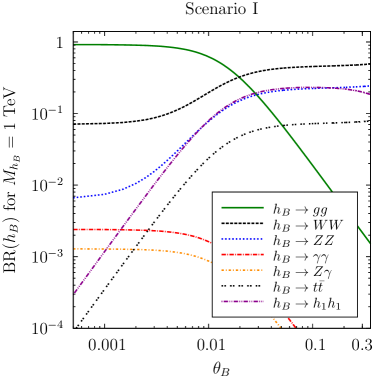
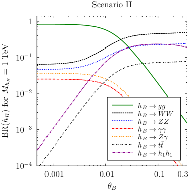
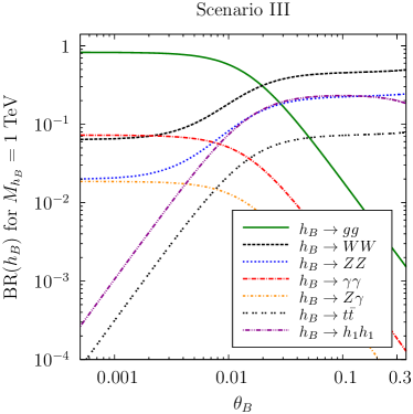
Figure 1: Branching ratios of the baryonic Higgs as a function of the mixing angle $\theta_{B}$ assuming only decays into SM particles. The vector-like quarks are assumed to be heavy and we use $v_{B}=2\,\mathrm{TeV}$ and $M_{h_{B}}=1\,\mathrm{TeV}$.

The new Higgs $h_{B}$ can decay into all particles present in the model, i.e.

$$h_{B}\to\bar{e}_{i}e_{i},\bar{q}_{i}q_{i},WW,ZZ,h_{1}h_{1},gg,\gamma\gamma,\bar{U}_{k}U_{k},\bar{D}_{k}D_{k},Z_{B}Z_{B},$$

where $i=1,2,3$ and $k=1,\ldots,6$. The properties of the decays depend in a significant way on the mixing angle between the SM Higgs and the new Higgs.

In Figure 1 we show the branching ratios of the baryonic Higgs into SM fields as a function of the Higgs mixing angle in the three scenarios. We use $M_{h_{B}}=1\,\mathrm{TeV}$ for illustration purposes. For large mixing angles close to the upper bound, the tree-level decays via mixing with the SM Higgs dominate, while for small mixing angles the loop-induced decays take over. In addition to the decay channels shown, tree-level decays into the leptophobic gauge boson are possible if the new Higgs is heavy enough. Depending on the mass hierarchy, it can also decay to some or all of the new quarks. For Figure 1 we have assumed that the new quarks are heavy so that these decays are not allowed. One can appreciate that for $\theta_{B}<0.02$ one has a large branching ratio into two gluons, while for $\theta_{B}>0.02$ the decays into $WW$ dominate.

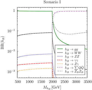
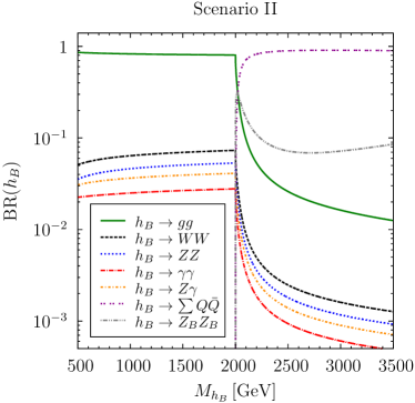
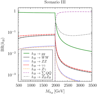
Figure 2: Branching ratios of the baryonic Higgs as a function of its mass $M_{h_{B}}$ assuming negligible mixing angle $\theta_{B}$. We use $M_{Z_{B}}=1\,\mathrm{TeV}$, $v_{B}=20\,\mathrm{TeV}$ and $m_{Q}=1\,\mathrm{TeV}$.

For a negligible mixing angle between the SM Higgs and the baryonic Higgs, the branching ratios of the baryonic Higgs are shown in Figure 2 for the three scenarios and all possible decay modes. One can see that in all scenarios the decays into gluons dominate in the range where the decays into vector-like quarks are not allowed, and for $M_{h_{B}}>2m_{Q}$ the decays in two vector-like quarks are dominant. For simplicity we assume throughout the article that all new vector-like quarks have the same mass $m_{Q}$. Notice that in the second and third scenario the decays into two photons can have a large branching ratio, much larger than $\text{BR}(h_{1}\to\gamma\gamma)$ in the SM. Also the branching ratio $\text{BR}(h_{B}\to Z\gamma)$ is large in scenarios II and III. These results are crucial to understand the constraints from the different search channels that we will discuss later.

III.2 Baryonic Higgs Production Mechanisms at the LHC

The new Higgs $h_{B}$ can be produced through different mechanisms. We focus on the production channels which do not rely on a large mixing angle and can be used to test these models in a generic way. The $h_{B}$ can be produced through gluon fusion, $gg\to h_{B}$, through vector-boson fusion via the $Z_{B}$, $q\bar{q}\to q\bar{q}h_{B}$, and one can have the associated production of $h_{B}$ and the leptophobic gauge boson $Z_{B}$, $pp\to Z_{B}^{*}\to Z_{B}h_{B}$. The associated production with two new quarks is also possible.

Since the masses of the vector-like quarks are generated once $S_{B}$ acquires a vev, the couplings between $h_{B}$ and the new quarks are typically large. Therefore, one can produce $h_{B}$ through gluon fusion where the vector-like quarks are running in the loop and this is the dominant production mechanism at the LHC. The production cross section for this channel is given by

$$\sigma\left(pp\to h_{B}\right)=\frac{C_{gg}}{sM_{h_{B}}}\Gamma\left(h_{B}\to gg\right).$$ (20)

Here, $C_{gg}$ is the gluonic PDF contribution, and we use the MSTW2008NLO PDFs Martin:2009iq in the remainder of this article, and $s$ is the center-of-mass energy squared. As we have discussed above, the branching ratio into two gauge bosons can be large. In particular, in scenarios II and III we expect a large number of events with two photons in the final state.

III.3 Experimental Constraints and Signatures

The cross section for the new Higgs being produced through gluon fusion and decaying into two SM gauge bosons $V$ is given by

$$\sigma_{VV}\equiv\sigma(pp\to h_{B})\times\text{BR}(h_{B}\to V\,V)\approx\frac{C_{gg}}{s}\frac{2\,\alpha_{s}^{2}\,M_{h_{B}}^{2}n_{f}^{2}}{9\pi^{3}v_{B}^{2}}\text{BR}(h_{B}\to V\,V),$$ (21)

where $n_{f}=3$ is the number of generations of vector-like quarks. This expression is general for the case that the new vector-like quark generation lives in the fundamental representation of $SU(3)_{C}$ and is heavy compared to the baryonic Higgs. We can use Eq. (21) to place a limit on the branching ratio of the new Higgs into two gauge bosons using the current LHC results from diboson searches.

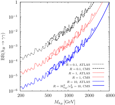
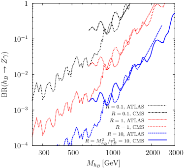
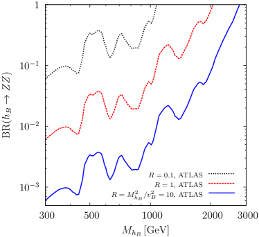
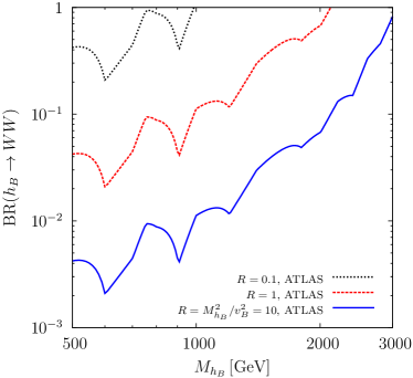
Figure 3: Constraints on the branching ratios of $h_{B}$ into two photons ATLAS:2016eeo ; Khachatryan:2016yec , $Z\gamma$ CMS:2016cbb ; ATLAS:2016lri , $ZZ$ ATLAS:2016npe , and $WW$ ATLAS:2016cwq for different choices of the ratio between mass and vev of the baryonic Higgs field. In the plots $n_{f}=3$.

In Figure 3 we show the upper limits on the branching ratios for the $\gamma\gamma$ ATLAS:2016eeo ; Khachatryan:2016yec , $Z\gamma$ CMS:2016cbb ; ATLAS:2016lri , $ZZ$ ATLAS:2016npe , and $WW$ ATLAS:2016cwq channels. Notice that these bounds are valid for all scenarios since the new vector-like quarks live in the fundamental representation of the QCD gauge group. These bounds are non-trivial even when we change the ratio $R=M_{h_{B}}^{2}/v_{B}^{2}$ between 0.1 and 10.

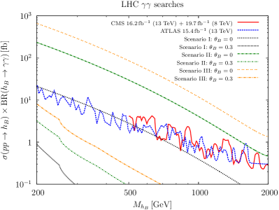
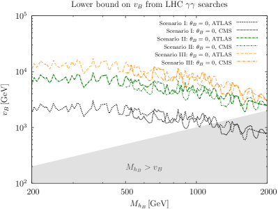
Figure 4: Constraints from diphoton searches ATLAS:2016eeo ; Khachatryan:2016yec . Left panel: experimental bounds as well as cross section predictions in scenarios I, II, and III as a function of the baryonic Higgs mass. Cross sections are shown both for negligible mixing angle and for a near maximal value of $\theta_{B}=0.3$. Right panel: experimental bounds translated into lower limits on $v_{B}$ as a function of $M_{h_{B}}$ for the case of negligible mixing. In the left panel we use $v_{B}=2\,\mathrm{TeV}$, and in both panels $n_{f}=3$ and $m_{Q}=1\,\mathrm{TeV}$.

Let us now discuss the different channels, starting with the di-photon searches. Assuming that the vector-like quarks are heavier than the baryonic Higgs, it is a good approximation to write (for one fermion)

$$\Gamma(h_{B}\to\gamma\gamma)=\frac{9\alpha^{2}n_{f}^{2}\,Q^{4}\,M_{h_{B}}^{3}}{144\pi^{3}\,v_{B}^{2}}$$ (22)

for the decay width into two photons. Here, $Q$ is the electric charge of a vector-like quark running in the loop. In the left panel of Figure 4, we show the most current limits on the production of a resonance and decay into two photons from ATLAS ATLAS:2016eeo and CMS Khachatryan:2016yec . We also show the predicted cross sections in the three scenarios for a particular choice of parameters in the left panel. Note that the cross sections are largest for the case of negligible mixing angle and are considerably lower for a mixing angle close to the upper allowed value, $\theta_{B}=0.3$. Therefore, we translate the experimental bounds on the cross section into bounds on the vev only for $\theta_{B}=0$. The lower bounds on $v_{B}$ are strong in the region where $M_{h_{B}}<v_{B}$ and become weak only in the unphysical region where $M_{h_{B}}\gg v_{B}$. To show the transition between these two regimes, we shade $M_{h_{B}}>v_{B}$ in gray in the plots. As one can appreciate these bounds are highly non-trivial, notice that the least constrained scenario is scenario I where the hypercharge of the new quarks are the same as the hypercharges of the SM quarks. In scenarios II and III the bounds are very strong and the symmetry breaking scale $v_{B}$ has to be well above the electroweak scale.

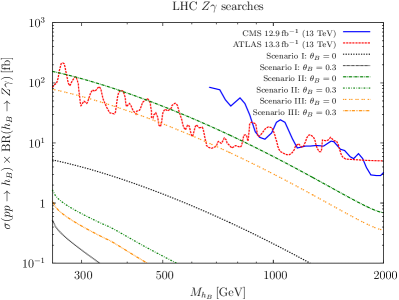
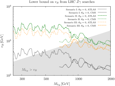
Figure 5: Constraints from $Z\gamma$ searches CMS:2016cbb ; ATLAS:2016lri . Left panel: experimental bounds as well as cross section predictions in scenarios I, II, and II as a function of the baryonic Higgs mass. Cross sections are shown both for negligible mixing angle and for a near maximal value of $\theta_{B}=0.3$. Right panel: experimental bounds translated into lower limits on $v_{B}$ as a function of $M_{h_{B}}$ for the case of negligible mixing. In the left panel we use $v_{B}=2\,\mathrm{TeV}$, and in both panels $n_{f}=3$ and $m_{Q}=1\,\mathrm{TeV}$.

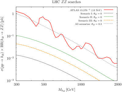
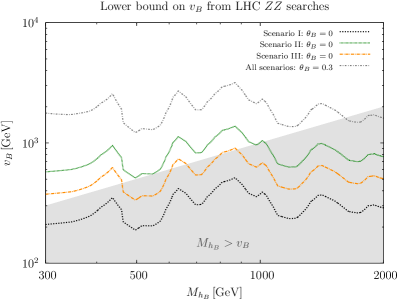
Figure 6: Constraints from $ZZ$ searches ATLAS:2016npe . Left panel: experimental bounds as well as cross section predictions in scenarios I, II, and II as a function of the baryonic Higgs mass. Cross sections are shown both for negligible mixing angle and for a near maximal value of $\theta_{B}=0.3$ for which the three scenarios coincide. Right panel: experimental bounds translated into lower limits on $v_{B}$ as a function of $M_{h_{B}}$. In the left panel we use $v_{B}=2\,\mathrm{TeV}$, and in both panels $n_{f}=3$ and $m_{Q}=1\,\mathrm{TeV}$.

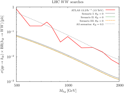
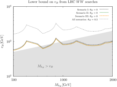
Figure 7: Constraints from $WW$ searches ATLAS:2016cwq . Left panel: experimental bounds as well as cross section predictions in scenarios I, II, and II as a function of the baryonic Higgs mass. Cross sections are shown both for negligible mixing angle and for a near maximal value of $\theta_{B}=0.3$ for which the three scenarios coincide. Right panel: experimental bounds translated into lower limits on $v_{B}$ as a function of $M_{h_{B}}$. In the left panel we use $v_{B}=2\,\mathrm{TeV}$, and in both panels $n_{f}=3$ and $m_{Q}=1\,\mathrm{TeV}$.

Other potentially relevant search channels are $Z\gamma$ CMS:2016cbb ; ATLAS:2016lri , $ZZ$ ATLAS:2016npe , and $WW$ ATLAS:2016cwq . Dijet searches turn out to be less constraining and will only be used for constraints on the leptophobic gauge boson in the next section. In Figures 5, 6, and 7 we show the bounds from the $Z\gamma$, $ZZ$ and $WW$ channels, respectively. As for the $\gamma\gamma$ channel, we shade the region where $M_{h_{B}}>v_{B}$ in gray. Notice that the bounds from $WW$ and $ZZ$ become relevant for large mixing angles, where $\gamma\gamma$ and $Z\gamma$ are heavily suppressed. Since the tree-level decays to $WW$ and $ZZ$ dominantly proceed via mixing with the SM Higgs in the case of a large mixing angle, the cross sections and experimental bounds for the three scenarios coincide for $\theta_{B}=0.3$

The result of the above discussion taking into account all current experimental bounds is that the symmetry breaking scale is highly constrained in most of the parameter space. For small mixing angle the most relevant bounds are from $\gamma\gamma$ searches and for large mixing angle the most relevant bounds are from $ZZ$ and $WW$ searches.

III.4 Leptophobic Gauge Boson

These theories predict the existence of a leptophobic gauge boson. The most stringent constraints on this new gauge boson come from dijet searches. In Ref. Fairbairn:2016iuf , dijet constraints were tabulated in a model-independent way and we use these to constrain the leptophobic gauge boson, together with more recent experimental results ATLAS:2016xiv ; CMS:2017xrr ; Aaboud:2017yvp . In this section we neglect kinetic mixing between $U(1)_{B}$ and $U(1)_{Y}$. For a detailed discussion of kinetic mixing in these models see Ref. Duerr:2014wra .

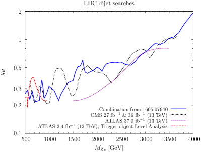
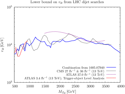
Figure 8: Current experimental constraints on leptophobic gauge bosons from dijet searches Fairbairn:2016iuf ; ATLAS:2016xiv ; CMS:2017xrr ; Aaboud:2017yvp . Left panel: upper bound on $g_{B}$ as a function of $M_{Z_{B}}$. Right panel: re-interpretation of the bounds in the mass–coupling plane as a lower bound on the symmetry breaking scale $v_{B}$.

In the left panel of Figure 8 we show the constraints in the $M_{Z_{B}}$–$g_{B}$ plane. These bounds assume that there are only decays into the SM quarks. If other decay channels are open, the bounds will be weaker. As we can see, the leptophobic gauge boson can be light when the gauge coupling $g_{B}$ is below 0.2. In the right panel of Figure 8 the gauge coupling limit is translated into a limit on the symmetry breaking scale. In combination with the need for a perturbative gauge coupling, $v_{B}$ cannot be smaller than $3.4\,\mathrm{TeV}$. We see that in the case of small scalar mixing the di-photon limits are competitive for all values of $M_{Z_{B}}$, compare with Figure 4. While for large scalar mixing the $WW$ and $ZZ$ channel are most sensitive to the symmetry breaking scale in the case of a heavy leptophobic gauge boson, compare to Figure 6.

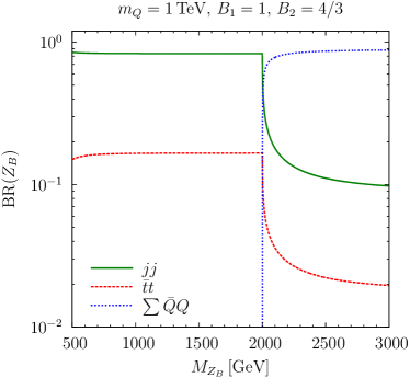
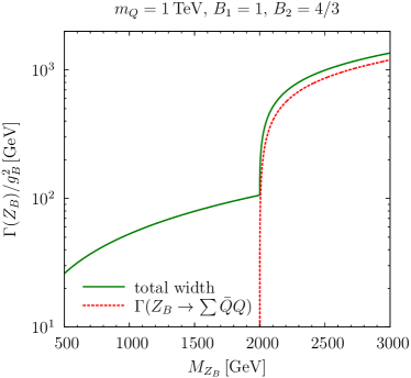
Figure 9: Branching ratios and total decay width of the leptophobic gauge boson. Here we assume $m_{Q}=1\,\mathrm{TeV}$, $B_{1}=1$ and $B_{2}=4/3$ for illustration. The decays into all SM quarks except for the top quarks are included in the $jj$ decays.

In order to understand the properties of the leptophobic gauge boson in these models we show in Figure 9 the branching ratios and the total width. As one can appreciate the dominant decay channel is the decay into quarks when the decays into the vector-like quarks are not allowed kinematically. Once the decays into vector-like quarks are allowed they dominate since they have larger baryon number. Here we assume $B_{1}=1$ and $B_{2}=4/3$ for illustration. It is interesting to see that the total decay width is quite large for any gauge coupling $g_{B}$. The discovery of this leptophobic gauge boson is crucial for the testability of these theories.

IV Summary

We have investigated the possible signatures at the Large Hadron Collider from decays of the new Higgs in simple extensions of the Standard Model where baryon number is a local symmetry spontaneously broken at the low scale. In this context one predicts the existence of a leptophobic gauge boson and a new CP-even Higgs boson associated to the spontaneous breaking of baryon number, as well as new vector-like quarks needed to cancel the baryonic anomalies.

The baryonic Higgs $h_{B}$ can decay into all the SM particles, the leptophobic gauge boson and into the vector-like quarks, giving rise to peculiar signatures at the LHC. We have investigated the constraints from $\gamma\gamma$, $Z\gamma$, $ZZ$, and $WW$ searches at the LHC. We find scenarios where the branching ratio into two photons can be large and one can have very striking signatures at the LHC. We also studied the properties of the leptophobic gauge boson present in these theories. We have shown that di-boson searches for the decays of the baryonic Higgs and di-jet searches for the leptophobic gauge boson are highly complementary and efficiently explore the parameter space of these theories. We find a lower bound one the symmetry breaking scale using the constraints from the di-photon searches. The signatures studied in the article are crucial to understand the testability of these theories at the LHC.

Appendix A Feynman Rules

$$\overline{U_{1}}U_{1}Z :\ -\frac{ie}{\sin 2\theta_{W}}\left(1-2\,Q_{u}\sin^{2}\theta_{W}\right)\gamma^{\mu},$$ (23)

$$\overline{U_{2}}U_{2}Z :\ i\,Q_{u}\,e\tan\theta_{W}\ \gamma^{\mu},$$ (24)

$$\overline{D_{1}}D_{1}Z :\ \frac{ie}{\sin 2\theta_{W}}\left(1+2Q_{d}\sin^{2}\theta_{W}\right)\ \gamma^{\mu},$$ (25)

$$\overline{D_{2}}D_{2}Z :\ iQ_{d}\,e\tan\theta_{W}\ \gamma^{\mu},$$ (26)

$$\overline{U_{i}}U_{i}A :\ -Q_{u}\,ie\,\gamma^{\mu},$$ (27)

$$\overline{D_{i}}D_{i}A :\ -Q_{d}\,ie\gamma^{\mu},$$ (28)

$$\overline{U_{k}}U_{k}h_{B} :\ i\frac{M_{U_{k}}}{v_{B}}\cos\theta_{B},$$ (29)

$$\overline{D_{k}}D_{k}h_{B} :\ i\frac{M_{D_{k}}}{v_{B}}\cos\theta_{B},$$ (30)

$$h_{1}h_{1}h_{B} :c_{11B}\equiv-6v_{0}\lambda_{H}\cos^{2}\theta_{B}\sin\theta_{B}+6v_{B}\lambda_{B}\cos\theta_{B}\sin^{2}\theta_{B}$$

$$\hphantom{:}+\lambda_{HB}\left(v_{B}\cos^{3}\theta_{B}+2v_{0}\cos^{2}\theta_{B}\sin\theta_{B}-2v_{B}\cos\theta_{B}\sin^{2}\theta_{B}-v_{0}\sin^{3}\theta_{B}\right).$$ (31)

Appendix B Decay Widths

B.1 Baryonic Higgs

The tree-level decay widths of the baryonic Higgs are given as follows. Here, $f$ denotes a SM fermion or a new quark.

$$\Gamma(h_{B}\to\bar{f}f) =\frac{N_{c}}{8\pi}|c_{h_{B}\bar{f}f}|^{2}M_{h_{B}}\left(1\ -\ 4\frac{M_{f}^{2}}{M_{h_{B}}^{2}}\right)^{3/2},$$ (32)

$$\Gamma(h_{B}\to h_{1}h_{1}) =\frac{1}{32\pi}\frac{|c_{11B}|^{2}}{M_{h_{B}}}\left(1-4\frac{M_{H_{1}}^{2}}{M_{h_{B}}^{2}}\right)^{1/2},$$ (33)

$$\Gamma(h_{B}\to WW) =\frac{G_{F}}{8\sqrt{2}\pi}\sin^{2}\theta_{B}\ M_{h_{B}}^{3}\left(1\ -\ 4\frac{M_{W}^{2}}{M_{h_{B}}^{2}}+12\frac{M_{W}^{4}}{M_{h_{B}}^{4}}\right)\left(1-4\frac{M_{W}^{2}}{M_{h_{B}}^{2}}\right)^{1/2},$$ (34)

$$\Gamma(h_{B}\to ZZ) =\frac{G_{F}}{16\sqrt{2}\pi}\sin^{2}\theta_{B}\ M_{h_{B}}^{3}\left(1\ -\ 4\frac{M_{Z}^{2}}{M_{h_{B}}^{2}}+12\frac{M_{Z}^{4}}{M_{h_{B}}^{4}}\right)\left(1-4\frac{M_{Z}^{2}}{M_{h_{B}}^{2}}\right)^{1/2},$$ (35)

$$\Gamma(h_{B}\to Z_{B}Z_{B}) =\frac{1}{32\pi}\frac{\cos^{2}\theta_{B}\ M_{h_{B}}^{3}}{v_{B}^{2}}\left(1\ -\ 4\frac{M_{Z_{B}}^{2}}{M_{h_{B}}^{2}}+12\frac{M_{Z_{B}}^{4}}{M_{h_{B}}^{4}}\right)\left(1-4\frac{M_{Z_{B}}^{2}}{M_{h_{B}}^{2}}\right)^{1/2}.$$ (36)

$c_{11B}$ is defined in the Feynman rules in Appendix. A. $c_{h_{B}\bar{f}f}$ is the coupling of the baryonic Higgs to the fermion $f$, which is given by

$$c_{h_{B}\bar{f}f}=\frac{M_{f}}{v_{0}}\sin\theta_{B}$$ (37)

for SM fermions and

$$c_{h_{B}\bar{f}f}=\frac{M_{f}}{v_{B}}\cos\theta_{B}$$ (38)

for the new vector-like quarks.

The loop-induced partial decay widths to SM gauge bosons of the new Higgs boson $h_{B}$ under the assumption that there is only negligible mixing with the SM Higgs are given in Appendix B of Ref. Duerr:2016eme and will not be repeated here. We used Package-X Patel:2015tea ; Patel:2016fam for the calculation of one-loop integrals. If there is non-negligible mixing with the SM Higgs, also SM particles will run in the loops, and corresponding formulas can for example be found in Ref. Djouadi:2005gi .

B.2 Leptophobic gauge boson

The partial decay width of the leptophobic gauge boson $Z_{B}$ to SM quarks is given by

$$\Gamma(Z_{B}\rightarrow\bar{q}q)=\frac{g_{B}^{2}}{36\pi}M_{Z_{B}}\left(1-\frac{4M_{q}^{2}}{M_{Z_{B}}^{2}}\right)^{\frac{1}{2}}\left(1+\frac{2M_{q}^{2}}{M_{Z_{B}}^{2}}\right),$$ (39)

while the decay width to vector-like quarks $Q$ with mass $m_{Q}$ is given by

$$\Gamma(Z_{B}\rightarrow\bar{Q}Q)=\frac{g_{B}^{2}}{8\pi}M_{Z_{B}}\left(1-\frac{4m_{Q}^{2}}{M_{Z_{B}}^{2}}\right)^{\frac{1}{2}}\left[\left(B_{1}^{2}+B_{2}^{2}\right)\left(1-\frac{m_{Q}^{2}}{M_{Z_{B}}^{2}}\right)+6B_{1}B_{2}\frac{m_{Q}^{2}}{M_{Z_{B}}^{2}}\right].$$ (40)

References

- (1) C. Patrignani et al. [Particle Data Group], “Review of Particle Physics,” Chin. Phys. C 40 (2016) 100001.
- (2) T. D. Lee and C. N. Yang, “Conservation of Heavy Particles and Generalized Gauge Transformations,” Phys. Rev. 98 (1955) 1501.
- (3) A. Pais, “Remark on baryon conservation,” Phys. Rev. D 8 (1973) 1844.
- (4) S. Rajpoot, “Gauge Symmetries Of Electroweak Interactions,” Int. J. Theor. Phys. 27 (1988) 689.
- (5) R. Foot, G. C. Joshi and H. Lew, “Gauged Baryon and Lepton Numbers,” Phys. Rev. D 40 (1989) 2487.
- (6) C. D. Carone and H. Murayama, “Realistic models with a light U(1) gauge boson coupled to baryon number,” Phys. Rev. D 52 (1995) 484 [arXiv:hep-ph/9501220].
- (7) P. Fileviez Perez and M. B. Wise, “Baryon and lepton number as local gauge symmetries,” Phys. Rev. D 82 (2010) 011901 [Erratum: Phys. Rev. D 82 (2010) 079901] [arXiv:1002.1754 [hep-ph]].
- (8) P. Fileviez Perez and M. B. Wise, “Breaking Local Baryon and Lepton Number at the TeV Scale,” JHEP 08 (2011) 068 [arXiv:1106.0343 [hep-ph]].
- (9) M. Duerr, P. Fileviez Perez and M. B. Wise, “Gauge Theory for Baryon and Lepton Numbers with Leptoquarks,” Phys. Rev. Lett. 110 (2013) 231801 [arXiv:1304.0576 [hep-ph]].
- (10) P. Fileviez Perez, S. Ohmer and H. H. Patel, “Minimal Theory for Lepto-Baryons,” Phys. Lett. B 735 (2014) 283 [arXiv:1403.8029 [hep-ph]].
- (11) P. Fileviez Perez, “New Paradigm for Baryon and Lepton Number Violation,” Phys. Rept. 597 (2015) 1 [arXiv:1501.01886 [hep-ph]].
- (12) P. Fileviez Perez and S. Ohmer, “Unification and Local Baryon Number,” Phys. Lett. B 768 (2017) 86 [arXiv:1612.07165 [hep-ph]].
- (13) B. Fornal, A. Rajaraman and T. M. P. Tait, “Baryon Number as the Fourth Color,” Phys. Rev. D 92 (2015) 055022 [arXiv:1506.06131 [hep-ph]].
- (14) T. R. Dulaney, P. Fileviez Perez and M. B. Wise, “Dark Matter, Baryon Asymmetry, and Spontaneous B and L Breaking,” Phys. Rev. D 83 (2011) 023520 [arXiv:1005.0617 [hep-ph]].
- (15) M. Duerr and P. Fileviez Perez, “Baryonic Dark Matter,” Phys. Lett. B 732 (2014) 101 [arXiv:1309.3970 [hep-ph]].
- (16) P. Fileviez Pérez and H. H. Patel, “Baryon Asymmetry, Dark Matter and Local Baryon Number,” Phys. Lett. B 731 (2014) 232 [arXiv:1311.6472 [hep-ph]].
- (17) M. Duerr and P. Fileviez Perez, “Theory for Baryon Number and Dark Matter at the LHC,” Phys. Rev. D 91 (2015) 095001 [arXiv:1409.8165 [hep-ph]].
- (18) S. Ohmer and H. H. Patel, “Leptobaryons as Majorana Dark Matter,” Phys. Rev. D 92 (2015) 055020 [arXiv:1506.00954 [hep-ph]].
- (19) P. Fileviez Perez and S. Ohmer, “Low Scale Unification of Gauge Interactions,” Phys. Rev. D 90 (2014) 037701 [arXiv:1405.1199 [hep-ph]].
- (20) M. Duerr, P. Fileviez Perez and J. Smirnov, “Gamma Lines from Majorana Dark Matter,” Phys. Rev. D 93, 023509 (2016) [arXiv:1508.01425 [hep-ph]].
- (21) M. Duerr, P. Fileviez Perez and J. Smirnov, “New Forces and the 750 GeV Resonance,” arXiv:1604.05319 [hep-ph].
- (22) M. Kusakabe, G. J. Mathews, T. Kajino, M. K. Cheoun, M. Kusakabe, G. J. Mathews, T. Kajino and M.-K. Cheoun, “Review on Effects of Long-lived Negatively Charged Massive Particles on Big Bang Nucleosynthesis,” arXiv:1706.03143.
- (23) M. Duerr, F. Kahlhoefer, K. Schmidt-Hoberg, T. Schwetz and S. Vogl, “How to save the WIMP: global analysis of a dark matter model with two s-channel mediators,” JHEP 09 (2016) 042 [arXiv:1606.07609 [hep-ph]].
- (24) G. Aad et al. [ATLAS and CMS Collaborations], “Measurements of the Higgs boson production and decay rates and constraints on its couplings from a combined ATLAS and CMS analysis of the LHC pp collision data at and 8 TeV,” JHEP 08 (2016) 045 [arXiv:1606.02266 [hep-ex]].
- (25) A. D. Martin, W. J. Stirling, R. S. Thorne and G. Watt, “Parton distributions for the LHC,” Eur. Phys. J. C 63 (2009) 189 [arXiv:0901.0002 [hep-ph]].
- (26) ATLAS Collaboration, “Search for scalar diphoton resonances with 15.4 fb-1 of data collected at in 2015 and 2016 with the ATLAS detector,” ATLAS-CONF-2016-059.
- (27) V. Khachatryan et al. [CMS Collaboration], “Search for high-mass diphoton resonances in proton-proton collisions at 13 TeV and combination with 8 TeV search,” Phys. Lett. B 767 (2017) 147 [arXiv:1609.02507 [hep-ex]].
- (28) CMS Collaboration, “Search for high-mass resonances in final state in pp collisions at with ,” CMS-PAS-EXO-16-035.
- (29) ATLAS Collaboration, “Search for new resonances decaying to a boson and a photon in 13.3 fb-1 of collisions at TeV with the ATLAS detector,” ATLAS-CONF-2016-044.
- (30) ATLAS Collaboration, “Searches for heavy ZZ and ZW resonances in the llqq and vvqq final states in pp collisions at sqrt(s) = 13 TeV with the ATLAS detector,” ATLAS-CONF-2016-082.
- (31) ATLAS collaboration, “Search for diboson resonance production in the final state using collisions at TeV with the ATLAS detector at the LHC,” ATLAS-CONF-2016-062.
- (32) M. Fairbairn, J. Heal, F. Kahlhoefer and P. Tunney, “Constraints on Z’ models from LHC dijet searches and implications for dark matter,” JHEP 09 (2016) 018 [arXiv:1605.07940 [hep-ph]].
- (33) ATLAS Collaboration, “Search for light dijet resonances with the ATLAS detector using a Trigger-Level Analysis in LHC pp collisions at TeV,” ATLAS-CONF-2016-030.
- (34) CMS Collaboration, “Searches for dijet resonances in pp collisions at using data collected in 2016,” CMS-PAS-EXO-16-056.
- (35) M. Aaboud et al. [ATLAS Collaboration], “Search for new phenomena in dijet events using 37 fb-1 of collision data collected at 13 TeV with the ATLAS detector,” arXiv:1703.09127 [hep-ex].
- (36) H. H. Patel, “Package-X: A Mathematica package for the analytic calculation of one-loop integrals,” Comput. Phys. Commun. 197 (2015) 276 [arXiv:1503.01469 [hep-ph]].
- (37) H. H. Patel, “Package-X 2.0: A Mathematica package for the analytic calculation of one-loop integrals,” arXiv:1612.00009 [hep-ph].
- (38) A. Djouadi, “The Anatomy of electro-weak symmetry breaking. I: The Higgs boson in the standard model,” Phys. Rept. 457 (2008) 1 [arXiv:hep-ph/0503172].