Lamb’s reconstruction of potentials and spatially localized scattering in nonrelativistic quantum mechanics

Abstract

We formulate a simple condition for reconstructibility of a certain class of Hamiltonians with real potentials from the knowledge of their complex-valued eigenfunctions. This may be relevant to the question of preparability of quantum states raised by W. Lamb in his 1969 paper on operational interpretation of quantum mechanics. Of particular interest to engineering applications are: (a) an exotic case of an upside-down harmonic-oscillator-type potential (a variation of the inverted “Mexican hat” potential) whose square-integrable complex eigenfunction describes a localized scattering state similar to the “bound state in the continuum” of von Neumann and Wigner, and (b) a spatially confined scattering state of a particle moving in an infinite well with the properly shaped potential bottom.

I Introduction

In 1969, Willis Lamb, Jr., published a remarkable paper Lamb1969 (also Lamb1979 ) on the operational foundations of nonrelativistic quantum mechanics, in which he proposed, among other things, an experimental procedure for preparing an arbitrary quantum state, $\psi(x)=R(x)e^{iS(x)}$, of a particle moving on the $x$-axis. The main assumption that had to be made in Ref. Lamb1969 was the availability of an arbitrary potential field, $V(x,t)$, with which to manipulate the corresponding quantum system. The preparation procedure consisted of the following four steps:

1. calculating, on the basis of $\psi(x)$, of a certain physically realizable potential, $V_{1}(x)$,

2. experimentally setting up the calculated $V_{1}(x)$,

3. catching the particle in one of the eigenstates, $\psi_{1}(x)\equiv R(x)$, of the resulting Hamiltonian, and, once the particle was caught,

4. subjecting the particle to an additional pulse perturbation of the form $-S(x)\delta(t)$, which, as seen from the time-dependent Schrödinger equation,

   $$i\frac{\partial\psi(x,t)}{\partial t}=-\frac{1}{2}\frac{\partial^{2}\psi(x,t)}{\partial x^{2}}-S(x)\delta(t)\psi(x,t),$$ (1)

   would immediately bring the particle to the desired state $\psi(x)$.

The final step involving the pulsed perturbation complicated the preparation procedure. Lamb resorted to that step because the method by which $V_{1}(x)$ was calculated (see Sec. III), when applied directly to the complex $\psi(x)$, resulted in a complex and thus unphysical potential (at least, as far as non-$PT$-symmetric case is concerned Bender1998 ; Bender2005 ). As a result, if one wanted to shorten the procedure by dropping the final step, one had to restrict consideration to real eigenfunctions only. Such a restriction limits experimentalist’s ability to control the quantum system. It is therefore natural to attempt to bypass that restriction by expanding the set of experimentally available wave functions associated with real, physically realizable (at least, in principle), potentials. In the following sections we find the conditions that must be imposed on a complex wave function in order for it to be an eigenfunction of a Hamiltonian with real potential. The set of the corresponding potentials turns out to be quite limited and consists of rather exotic field configurations that are not typically encountered in a laboratory.

II Formulation of the problem

In one dimension, the task is: Given a complex wave function, $\psi(x)$, reconstruct the Hamiltonian, $H$, for which that function is an eigenfunction.

The Hamiltonian is assumed to be of the form

$$H=-\frac{1}{2}\frac{d^{2}}{dx^{2}}+V(x),$$ (2)

with the corresponding time-independent Schrödinger’s equation being

$$-\frac{1}{2}\frac{d^{2}\psi(x)}{dx^{2}}+V(x)\psi(x)=E\psi(x).$$ (3)

The given eigenfunction is assumed to be

$$\psi(x)=R(x)e^{iS(x)},$$ (4)

with real $R(x)$ and $S(x)$, as proposed in Ref. Lamb1969 . To avoid problems with singular solutions, we restrict consideration to nodeless $R(x)$ only. The goal is to find a real potential $V(x)$ that satisfies both (3) and (4).

III Reconstruction Procedure

When $\psi(x)$ is real, the procedure due to Lamb Lamb1969 (and also Berezin, as recounted in Turbiner2016 ) is to simply invert (3) and get

$$V(x)=E+\frac{1}{2}\frac{\psi^{\prime\prime}(x)}{\psi(x)},$$ (5)

where $E$ can be chosen arbitrarily (the prime ^′ indicates differentiation with respect to $x$). When $\psi(x)$ is complex, this procedure fails (we do not get real $V(x)$), unless specific “reconstructability” conditions are satisfied. Our goal is to determine those conditions.

To determine the reconstructability conditions, we first notice that due to its linearity the Schrödinger equation (3) is separately satisfied by each of the real and imaginary parts of $\psi(x)$. Thus, writing

$$\psi(x)=a(x)+ib(x),$$ (6)

with real $a(x)$ and $b(x)$, we get

$$-\frac{1}{2}\frac{d^{2}a(x)}{dx^{2}}+V(x)a(x) =Ea(x),$$ (7)

$$-\frac{1}{2}\frac{d^{2}b(x)}{dx^{2}}+V(x)b(x) =Eb(x).$$ (8)

Inverting each of these equations automatically gives two real potentials,

$$V_{a}(x) =E+\frac{1}{2}\frac{a^{\prime\prime}(x)}{a(x)},$$ (9)

$$V_{b}(x) =E+\frac{1}{2}\frac{b^{\prime\prime}(x)}{b(x)},$$ (10)

and, since in both cases we must get the same $V(x)$, the sought reconstructability condition reads

$$\frac{a^{\prime\prime}(x)}{a(x)}=\frac{b^{\prime\prime}(x)}{b(x)}.$$ (11)

To recast (11) in terms of $R(x)$ and $S(x)$, we write

$$\psi(x) =R(x)\cos S(x)+iR(x)\sin S(x),$$ (12)

and find

$$\frac{a^{\prime\prime}}{a} \equiv\frac{(R\cos S)^{\prime\prime}}{R\cos S}=\frac{R^{\prime\prime}-R(S^{\prime})^{2}}{R}-\frac{2R^{\prime}S^{\prime}+RS^{\prime\prime}}{R}\tan S,$$ (13)

$$\frac{b^{\prime\prime}}{b} \equiv\frac{(R\sin S)^{\prime\prime}}{R\sin S}=\frac{R^{\prime\prime}-R(S^{\prime})^{2}}{R}+\frac{2R^{\prime}S^{\prime}+RS^{\prime\prime}}{R}\frac{1}{\tan S}.$$ (14)

Eq. (11) demands that in (13) and (14) we set

$$2R^{\prime}S^{\prime}+RS^{\prime\prime}=0,$$ (15)

which gives

$$S(x)=C\int^{x}\frac{ds}{R^{2}(s)},$$ (16)

where $C$ is an arbitrary real constant. Thus, for a given $R(x)$ in (4), we choose $S(x)$ in accordance with (16), and using (13) get the real potential (cf. vonNeumann1929 ; Stillinger1975 ; Khelashvili1996 ; Petrovic2002 ),

$$V(x)=E+\frac{R^{\prime\prime}}{2R}-\frac{C^{2}}{2R^{4}}.$$ (17)

This results in the Hamiltonian,

$$H=-\frac{1}{2}\frac{d^{2}}{dx^{2}}+\frac{R^{\prime\prime}}{2R}-\frac{C^{2}}{2R^{4}}+E,$$ (18)

whose complex eigenfunction of energy $E$ is given by

$$\psi(x)=R(x)\exp\left\{iC\int^{x}\frac{ds}{R^{2}(s)}\right\},$$ (19)

where the lower limit of integration may be chosen arbitrarily; different choices will result in unimportant phase shifts. For nodeless $R(x)$, the function $\psi(x)$ satisfies all the usual properties of a “legitimate” wave function LL1977 : it is single-valued and continuous on the entire $x$-axis. Additionally, if $R(x)$ is square-integrable, then so is the $\psi(x)$. The characteristic feature of all the found wave functions is that the associated current densities,

$$j_{x}(x)=R^{2}(x)S^{\prime}(x)=C,$$ (20)

are constant throughout their respective domains of definition.

In higher dimensions, the Schrödinger equation reads (here, ${\bf r}$ is particle’s position vector, $\nabla$ is the nabla operator)

$$-\frac{1}{2}\nabla^{2}\psi({\bf r})+V({\bf r})\psi({\bf r})=E\psi({\bf r}),$$ (21)

with the analogues of Eqs. (11) and (15) being, respectively,

$$\frac{\nabla^{2}a}{a}=\frac{\nabla^{2}b}{b},$$ (22)

and

$$2\nabla R\cdot\nabla S+R\nabla^{2}S=0.$$ (23)

For example, in the spherically symmetric case in three dimensions, we get

$$2\frac{dR}{dr}\frac{dS}{dr}+\frac{R}{r^{2}}\frac{d}{dr}\left(r^{2}\frac{dS}{dr}\right)=0,$$ (24)

which gives,

$$S(r)=C\int^{r}\frac{ds}{s^{2}R^{2}(s)},$$ (25)

and, thus,

$$V(r)=E+\frac{1}{2Rr^{2}}\frac{d}{dr}\left(r^{2}\frac{dR}{dr}\right)-\frac{C^{2}}{2r^{4}R^{4}},$$ (26)

with the corresponding eigenfunction being

$$\psi(r)=R(r)\exp\left\{iC\int^{r}\frac{ds}{s^{2}R^{2}(s)}\right\}.$$ (27)

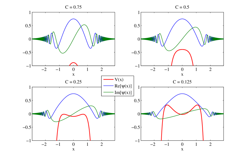
Figure 1: (Figure online.) Deformed harmonic-oscillator case of Sec. V, Eqs. (32) and (33): Plots of the reconstructed potential, $V(x)$, as well as the real and imaginary parts of its complex nodeless eigenfunction, $\psi(x)$, for several values of $C$. The lower limit of integration in (32) was set to zero. When $C=0$, we recover the standard harmonic oscillator result.

IV Example: Free particle in one dimension

The simplest example is provided by a wave function with prefactor

$$R(x)=1,$$ (28)

or,

$$\psi(x)=\exp\left\{iC\int_{0}^{x}ds\right\}=e^{iCx}.$$ (29)

The corresponding potential is immediately found to be

$$V(x)=0,$$ (30)

where we set $E=C^{2}/2$. This is the usual expression for particle’s kinetic energy in terms of its momentum $C$. Being trivial, this result serves as a useful consistency check for our approach.

V Example: One-dimensional Harmonic oscillator

Here we consider a localized wave function with prefactor

$$R(x)=\left(\frac{1}{\pi}\right)^{1/4}e^{-x^{2}/2},$$ (31)

so that

$$\psi(x)=\left(\frac{1}{\pi}\right)^{1/4}e^{-x^{2}/2}\exp\left\{iC\sqrt{\pi}\int_{0}^{x}e^{s^{2}}ds\right\}.$$ (32)

The corresponding potential, according to (17), is

$$V(x)=\frac{x^{2}}{2}-\frac{C^{2}\pi e^{2x^{2}}}{2},$$ (33)

where we set $E=1/2$. When $C=0$, we get the standard harmonic oscillator result. When $C\neq 0$, the harmonic oscillator potential deforms into an upside-down shape (a variation of inverted “Mexican hat” potential), as shown in Fig. 1, with the phase of the wave function rapidly increasing as $|x|\rightarrow\infty$. Thus, what we are dealing with here is a singular Sturm-Liouville problem with a negatively diverging potential, $V(x)\rightarrow-\infty$, on both ends of the corresponding boundary-value interval, $|x|\rightarrow\infty$. This is reminiscent of the situation encountered in $PT$-symmetric quantum mechanics Bender1998 , where some Hamiltonians, such as, e. g.,

$$H_{PT}={p^{2}}+x^{2}(ix)^{N},\quad N=2,$$ (34)

often come with upside-down potentials. The difference between the two approaches is that in our case the resulting Hamiltonian is Hermitian (in the standard Dirac’s sense) and does not require any redefinition of the usual scalar product on the Hilbert space of states.

The above result is unusual in that the probability current corresponding to (32) is, according to Sec. III, constant throughout the entire $x$-axis,

$$j_{x}=R^{2}S^{\prime}=C,$$ (35)

while the probability density,

$$\rho=R^{2}=\frac{e^{-x^{2}}}{\sqrt{\pi}},$$ (36)

is exponentially decreasing with the square of the distance from the origin. Eq. (35) is a signature of a scattering state. It shows that $\psi(x)$ represents a particle impinging from the left (if $C>0$) on the corresponding potential barrier and then accelerating away to (positive) infinity, while spending most of its “life” being localized on the barrier’s top (compare with the above-barrier localized states in double-well potentials considered in Refs. Dutta1992 ; Dutta1996 ; also see vonNeumann1929 ; Stillinger1975 ; Khelashvili1996 ; Petrovic2002 and Simon1967 ; Arai1999 for the so-called “bound states in the continuum” of von Neumann and Wigner).

A natural question arises whether the found potential (33) is physically realistic. Superficially, the answer seems to be “no,” since it is well-known that a classical particle subjected to a much milder potential $V(x)=-|x|^{\alpha}$ would reach infinity in finite time for any $\alpha>2$ (see, e. g., ReedSimonII , Simon2000 ), and out potential is much more singular than that. However, one should keep in mind that, from the physical standpoint, even the usual harmonic oscillator potential cannot be regarded as realistic, for there does not exist a system in nature for which $V(x)=x^{2}/2$ for all $x$. Nevertheless, the harmonic oscillator often serves as a useful approximation to actual, physically realizable situations: its first few states describe various quantum systems quite well. We expect something similar to take place with our singular potentials too. For example, as a useful approximation, we can construct a potential that has the form (33) on a finite interval, $|x|\leq a<+\infty$, and adjust the system parameters so that the real part of $\psi$ would vanish at $|x|=a$. The resulting configuration would then be indistinguishable from the one involving a particle confined to an infinite well with the walls at $x=\pm a$. Of course, such scenario is not as dramatic as the localized scattering on an infinite line. However, it may be possible to create some finite, physically realistic, periodic configurations (say, motion on a circle, such as in the case of superconducting Josephson phase qubits DM2004 ), whose quantum states exhibit properties similar to those of the localized scattering states considered above.

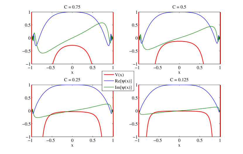
Figure 2: (Figure online.) Deformed infinite square well case of Sec. VI, Eqs. (38) and (39): Plots of the reconstructed potential, $V(x)$, as well as the real and imaginary parts of its nodeless complex eigenfunction, $\psi(x)$, for several values of $C$. The lower limit of integration in (19) was set to zero.

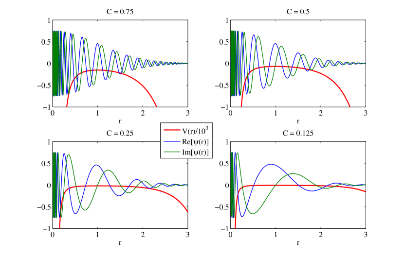
Figure 3: (Figure online.) Deformed hydrogen atom potential of Sec. VII, Eqs. (43) and (44): Plots of the reconstructed potential, $V(x)$, as well as the real and imaginary parts of its nodeless complex eigenfunction, $\psi(x)$, for several values of $C$. The lower limit of integration in (43) was set to 1.

VI Example: One-dimensional infinite square well

In this example, the prefactor is

$$R(x)=\cos\left(\frac{\pi x}{2}\right),\quad|x|<1,$$ (37)

which results in the eigenfunction

$$\psi(x)=\cos\left(\frac{\pi x}{2}\right)\exp\left\{iC\frac{2}{\pi}\tan\left(\frac{\pi x}{2}\right)\right\},\quad|x|<1.$$ (38)

The corresponding potential, according to (17), is

$$V(x)=-\frac{C^{2}}{2\cos^{4}\left(\frac{\pi x}{2}\right)},\quad|x|<1,$$ (39)

where we set $E=\pi^{2}/8$. When $C=0$, we recover the standard result for an infinite square well. When $C\neq 0$, the potential bottom assumes an upside-down shape, as shown in Fig. 2, with the phase of the wave function rapidly increasing as one approaches the infinite walls at $|x|=1$.

The probability current corresponding to (38) is constant throughout the interval $|x|\leq 1$,

$$j_{x}=C,$$ (40)

while the probability density varies with position as

$$\rho=\cos^{2}\left(\frac{\pi x}{2}\right).$$ (41)

In this case we have a scattering state confined in a box. Thinking classically, the particle always moves in one direction, never encountering the potential walls. This example complements rather nicely the remarks made at the end of the previous section.

VII Example: Hydrogen atom

Here we consider spherically symmetric prefactor,

$$R(r)=\frac{1}{\pi^{1/2}}e^{-r},$$ (42)

which gives the wave function,

$$\psi(r)=\frac{1}{\pi^{1/2}}e^{-r}\exp\left\{iC\pi\int^{r}_{1}\frac{e^{2s}}{s^{2}}ds\right\},$$ (43)

where we have conveniently set the lower limit of integration to 1 to avoid the singularity at the origin. The corresponding potential, according to (26), is (see Fig. 3)

$$V(r)=-\frac{1}{r}-\frac{C^{2}\pi^{2}e^{4r}}{2r^{4}},$$ (44)

where we have chosen $E=-1/2$. In this example, setting $C$ to zero reproduces the familiar ground state and Coulomb potential of the hydrogen atom.

VIII Conclusions

In summary, we have given a sufficient condition for Lamb’s reconstructability of certain real-valued potentials from the knowledge of their respective complex eigenfunctions. The found potentials are rather exotic and not typically encountered in nature. Nevertheless, as a matter of principle, our results could still be useful for designing new experimental techniques for quantum state preparation, manipulation, and control, as well as for the development of novel quantum electronic devices Vladimirova1999 ; Ordonez2006 ; Nakamura2007 ; Longhi2007 ; Moiseyev2009 ; Hsueh2010 ; Prodanovic2013 .

References

- (1) W. E. Lamb, Jr., “An operational interpretation of nonrelativistic quantum mechanics,” Phys. Today 22, 23 (1969).
- (2) W. E. Lamb, Jr., “Remarks on the interpretation of quantum mechanics,” in Science of Matter, edited by S. Fujita (Gordon and Breach, New York, 1979), pp. 1-8.
- (3) C. M. Bender and S. Boettcher, “Real Spectra in Non-Hermitian Hamiltonians Having PT-Symmetry,” Phys. Rev. Lett. 80, 5243 (1998).
- (4) C. M. Bender, “Introduction to -symmetric quantum theory,” Contemp. Phys. 46, 277 (2005).
- (5) A. V. Turbiner, “One-dimensional quasi-exactly solvable Schrödinger equations,” Phys. Rep. 642, 1 (2016).
- (6) J. von Neumann and E. Wigner, “Über merkwürdige diskrete Eigenwerte,” Phys. Z. 30, 465 (1929).
- (7) F. H. Stillinger and D. R. Herrick, “Bound states in the continuum,” Phys. Rev. A 11,446 (1975).
- (8) A. Khelashvili and N. Kiknadze, “Von Neumann - Wigner-type potentials and the wavefunctions’ asymptotics for discrete levels in continuum,” J. Phys. A 29, 3209 (1996).
- (9) J. S. Petrović, V. Milanović, Z. Ikonić, “Bound states in continuum of complex potentials generated by supersymmetric quantum mechanics,” Phys. Lett. A 300, 595 (2002).
- (10) L. D. Landau, E. M. Lifshitz, Quantum Mechanics, Course of Theoretical Physics Series, vol. 3 (Butterworth-Heinemann, 1977), 3rd ed.
- (11) P. Dutta, S. P. Bhattacharyya, “Localized quantum states on and above the top of a barrier,” Phys. Lett. A 163, 193 (1992).
- (12) S. Adhikari, S. P. Bhattacharyya, P. Dutta, “Stability of localized quantum states on the top of a barrier and some of its consequences: the specific case of a symmetric double well potential,” Chem. Phys. Lett. 248, 218 (1996).
- (13) B. Simon, “On Positive Eigenvalues of One-Body Schrodinger Operators,” Comm. Pure Appl. Math. XXII, 531 (1967).
- (14) M. Arai and J. Uchiyama, “On the von Neumann and Wigner Potentials,” J. Diff. Eq. 157, 348 (1999).
- (15) M. Reed and B. Simon, Methods of Modern Mathematical Physics, II. Fourier Analysis, Self-Adjointness (Academic, New York, 1975).
- (16) B. Simon, “Schroödinger operators in the twentieth century,” J. Math. Phys. 41, 3523 (2000).
- (17) M. Devoret and J. Martinis, “Superconducting Qubits,” in D. Esteve, J.-M. Raimond, J. Dalibard, Quantum Entanglement and Information Processing (Elsevier, 2004).
- (18) M. R. Vladimirova, A. V. Kavokin, M. A. Kaliteevskii, S. I. Kokhanovskii, M. E. Sasin, R. P. Seisyan, “Above-barrier excitons: First magnetooptic investigation,” J. Exp. Theor. Phys. Lett. 69, 779 (1999).
- (19) G. Ordonez, K. Na, and S. Kim, “Bound states in the continuum in quantum-dot pairs,” Phys. Rev. A 73, 022113 (2006).
- (20) H. Nakamura, N. Hatano, S. Garmon, and T. Petrosky, “Quasibound States in the Continuum in a Two Channel Quantum Wire with an Adatom,” Phys. Rev. Lett. 99, 210404 (2007).
- (21) S. Longhi, “Bound states in the continuum in a single-level Fano-Anderson model,” Eur. Phys. J. B 57, 45 (2007).
- (22) N. Moiseyev, “Suppression of Feshbach Resonance Widths in Two-Dimensional Waveguides and Quantum Dots: A Lower Bound for the Number of Bound States in the Continuum,” Phys. Rev. Lett. 102, 167404 (2009).
- (23) W. J. Hsueh, C. H. Chen, C. H. Chang, “Bound states in the continuum in quasiperiodic systems,” Phys. Lett. A 374, 4804 (2010).
- (24) N. Prodanović, V. Milanović, Z. Ikonić, D. Indjina, P. Harrison, “Bound states in continuum: Quantum dots in a quantum well,” Phys. Lett. A 377, 2177 (2013).