Existence and instability of steady states for a triangular cross-diffusion system: a computer-assisted proof

Abstract

In this paper, we present and apply a computer-assisted method to study steady states of a triangular cross-diffusion system. Our approach consist in an a posteriori validation procedure, that is based on using a fixed point argument around a numerically computed solution, in the spirit of the Newton-Kantorovich theorem. It allows us to prove the existence of various non homogeneous steady states for different parameter values. In some situations, we get as many as 13 coexisting steady states. We also apply the a posteriori validation procedure to study the linear stability of the obtained steady states, proving that many of them are in fact unstable.

Key words Rigorous numerics $\cdot$ Cross-diffusion $\cdot$ Steady states
Eigenvalue problem $\cdot$ Spectral analysis $\cdot$ Fixed point argument

1 Introduction

The primary goal of describing physical systems with mathematical models is to be able to explain and predict natural phenomena, within some range of approximation. In some circumstances the mathematical prediction and the experimental evidence don’t agree, and a more trustful model is then required. Typically, one can add nonlinear or non homogeneous terms to get a more refined model, but this often seriously complicates the mathematical analysis of the system, which can become very hard, if not impossible, to study analytically. In this situation, numerical simulations allow insight of the phenomena and provide approximate, often very accurate, solutions. Aiming at formulating theorems, a powerful tool to validate approximate solutions into rigorous mathematical statements is provided by the rigorous computational techniques.

The diffusive Lotka-Volterra system, a well known model for population dynamics to study the competition between two species, is paradigmatic of the situation discussed above. It consists in the system

$$\left\{\begin{aligned} &\frac{\partial u}{\partial t}=d_{1}\Delta u+(r_{1}-a_{1}u-b_{1}v)u,\quad&\text{on }\mathbb{R}_{+}\times\Omega,\\ &\frac{\partial v}{\partial t}=d_{2}\Delta v+(r_{2}-b_{2}u-a_{2}v)v,\quad&\text{on }\mathbb{R}_{+}\times\Omega,\\ &\frac{\partial u}{\partial n}=0=\frac{\partial v}{\partial n},\quad\text{on }\mathbb{R}_{+}\times\partial\Omega,\end{aligned}\right.$$ (1)

where $\Omega$ is a bounded domain of $\mathbb{R}^{N}$, and $u(t,x),v(t,x)\geq 0$ represent the population densities of two species at time $t$ and position $x$. The non negative coefficients $d_{i}$, $r_{i}$, $a_{i}$ and $b_{i}$ ($i=1,2$) describe the diffusion, the unhindered growth of the species, the intra-specific competition and the inter-specific competition respectively.

One of the fundamental problems is to determine if and under which assumptions the two species coexist, that converts into proving the existence or non-existence of stable positive equilibrium solutions. Several works has been produced to classify and analyse the stability of the equilibria for (1) and of related systems. We refer for instance to [38] for a short review. Of particular interest for our discussion is the result presented in [31]. If the domain $\Omega$ is convex, in that paper it is proved that any spatially non-constant equilibrium solution of (1) is unstable, if it exists. This implies that if the two species coexist, their densities must be homogeneous in the whole domain.

However, biological observations suggest that two competing species could coexist by forming pattern to avoid each other (a phenomenom called spatial segregation). Therefore we would like the model to exhibit stable non homogeneous steady states, but the quoted result shows that this is excluded (at least for convex domains). We point out that stable non homogeneous equilibria have been shown to exist for non convex domains [36], or for systems involving more than two species [30].

In the case of two competing species, to account for the expected stable inhomogeneous steady sates, a generalization of (1) was proposed in [47]:

$$\left\{\begin{aligned} &\frac{\partial u}{\partial t}=\Delta((d_{1}+d_{12}v)u)+(r_{1}-a_{1}u-b_{1}v)u,\quad\text{on }\mathbb{R}_{+}\times\Omega,\\ &\frac{\partial v}{\partial t}=\Delta((d_{2}+d_{21}u)v)+(r_{2}-b_{2}u-a_{2}v)v,\quad\text{on }\mathbb{R}_{+}\times\Omega,\\ &\frac{\partial u}{\partial n}=0=\frac{\partial v}{\partial n},\quad\text{on }\mathbb{R}_{+}\times\partial\Omega,\end{aligned}\right.$$ (2)

where the added cross-diffusion terms $\Delta(uv)$ model that the two species try to avoid each other, by diffusing more when more individuals of the other species are present.

Since its introduction the system (2) has been studied extensively, one of the main reason being that it seems to exhibit a much wider variety of steady states than (1), especially non homogeneous ones, in accordance to laboratory experiments. Several numerical studies have been presented, displaying intricate bifurcation diagrams of steady states (see for instance [26, 27] and also Figure 1). Consider for instance the homogenous equilibria

$$(u_{eq},v_{eq}):=\left(\frac{r_{1}a_{2}-r_{2}b_{1}}{a_{1}a_{2}-b_{1}b_{2}},\frac{r_{2}a_{1}-r_{1}b_{2}}{a_{1}a_{2}-b_{1}b_{2}}\right)$$ (3)

in the strong intra-specific case, i.e. when $\frac{b_{1}}{a_{2}}<\frac{r_{1}}{r_{2}}<\frac{a_{1}}{b_{2}}$ (the other case $\frac{a_{1}}{b_{2}}<\frac{r_{1}}{r_{2}}<\frac{b_{1}}{a_{2}}$ is known as the strong inter-specific competition case). While $(u_{eq},v_{eq})$ is stable for (1) for any diffusion coefficient $d_{1},d_{2}\geq 0$, adding strong enough cross-diffusion can destabilize this equilibria, from which new non homogeneous steady states can bifurcate. A link between this cross-diffusion induced instability and the standard Turing instability for reaction-diffusion systems is made in [26].

While from one side the addition of these nonlinear cross-diffusion terms yields a more reliable model, on the other it seriously complicates the analytical treatment of the system. Even the existence of global classical solutions of (2) (completed with non negative initial data) is a challenging question that is still fairly open. Local in time existence can be obtained by the theory of quasilinear parabolic systems [1], but to then get bounds that prevent blowups requires restrictions on the coefficients, as for instance $d_{21}=0$ [17]. In this particular case, sometimes called triangular cross-diffusion system, some recent progresses were also made in [20] by combining entropy methods with a 3 component reaction-diffusion system without cross-diffusion (first introduced in [26]), that is used to approach (2). Entropy methods were also used to improve upon the existing results for the full cross-diffusion system, see [28, 19] and the references therein.

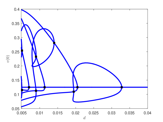
Figure 1: A numerical bifurcation diagram of steady states of (2), in the strong intra-specific case. The space domain $\Omega$ is $(0,1)$, $r_{1}=5$, $r_{2}=2$, $a_{1}=3$, $a_{2}=3$, $b_{1}=1$, $b_{2}=1$, $d_{12}=3$, $d_{21}=0$ and $d_{1}=d_{2}=d$ is left as the bifurcation parameter.

Existence and stability results for non homogeneous steady states of (2) have also been established following different approaches including bifurcations techniques [39], singular perturbation techniques [40, 35] and fixed point index theory [46]. Because of the presence of the cross-diffusion term, the analytical studies are limited to those solutions that are either close the homogeneous steady states, or in very specific parameter ranges. However, the numerically computed bifurcation diagram reveals a very rich structure that includes coexistence of many different steady states for a given set of parameter values, as well as secondary bifurcations. To the best of the author’s knowledge, even the existence of these solutions is not yet proved and it seems out of reach of purely analytical techniques.

The aim of this paper is to prove existence and study the linear stability of several non-homogenous steady states of (2), significantly far from being perturbations of the homogeneous equilibria, also showing multiplicity of solutions for the same set of parameters. The kind of technique adopted here is often referred to as validated numerics, because the goal is to prove the existence of a genuine solution of the problem in a sharp and explicit neighborhood of a numerical one, hence, in this sense, to validate the approximate solution (more details in Section 2). More precisely, we follow the so called radii polynomial approach, a quite general technique based on the contraction mapping argument that has been adapted to solve several differential problems in areas ranging from dynamical systems to ordinary and partial differential equations through delay differential equation and chaotic dynamics. This is the first time that rigorous computational techniques are applied to PDE system with cross interactions in the leading differential operator. The cross-diffusion terms are indeed a major technical hurdles, since they enfeeble the smoothing effect of the higher order differential operator.

In this work we restrict ourself to the triangular case and assume that the space dimension is 1 (i.e. we fix $d_{21}=0$ and $\Omega=(0,1)$). The method can easily be extended to higher space dimension (say 2 or 3), but of course the computational cost would increase. The generalization to a full cross-diffusion system is less straightforward. Indeed, as mentioned above, it will become apparent in the next sections that the cross-diffusion structure hinders the use of our validation method, and that we take advantage of the triangular configuration to overcome this difficulty.

The system we are dealing with is the following:

$$\left\{\begin{aligned} &\!\left((d_{1}+d_{12}v)u\right)^{\prime\prime}+(r_{1}-a_{1}u-b_{1}v)u=0,\quad&\text{on }(0,1),\\ &d_{2}v^{\prime\prime}+(r_{2}-b_{2}u-a_{2}v)v=0,\quad&\text{on }(0,1),\\ &u^{\prime}(0)=u^{\prime}(1)=0,\\ &v^{\prime}(0)=v^{\prime}(1)=0.\end{aligned}\right.$$ (4)

Figure 1 depicts a bifurcation diagram of solutions of (4), with given values for the parameters $r_{i}$, $a_{i}$, $b_{i}$ and $d_{12}$. This diagram was first obtained numerically in [26], using a 3-component system without cross-diffusion that approaches (4). We point out that even in the somewhat restricted framework with $\Omega=(0,1)$ and $d_{12}=0$, the steady states of (2) already manifest very complex and interesting behavior when the parameters vary.

The first result concerns the existence of steady states.

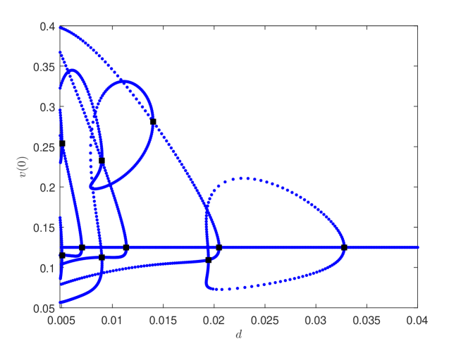
Figure 2: Validated bifurcation diagram of solutions of (4). The space domain $\Omega$ is $(0,1)$, $r_{1}=5$, $r_{2}=2$, $a_{1}=3$, $a_{2}=3$, $b_{1}=1$, $b_{2}=1$, $d_{12}=3$, and $d_{1}=d_{2}=d$ is left as the bifurcation parameter. Each blue dot represents a proved solution. The black squares indicate bifurcations, while the other apparent crossings are just due to the projection (i.e. $v(0)$) we used to represent the solutions.

Theorem 1.1.

Referring to Figure 2, each bullet represents a solution of (4), for the parameter values $r_{1}=5$, $r_{2}=2$, $a_{1}=3$, $a_{2}=3$, $b_{1}=1$, $b_{2}=1$, $d_{12}=3$, and $d_{1}=d_{2}=d$. In particular there exists at least 13 different solutions when $d_{1}=d_{2}=0.005$.

The proof of each steady states also provides precise qualitative informations about the solution, in terms of explicit bounds of the distance (in some function space, see Section 4) between the genuine solution that is proved to exist and a numerically computed approximation (more details in Section 5).

In [26], the linear stability of the obtained steady states was also studied (still numerically), suggesting that most of the solutions displayed in the bifurcation diagram of Figure 2 are unstable, while others seems to be stable. In this direction, the second contribution of this paper is a rigorous computational approach to the study of the spectral properties of the equilibria presented above.

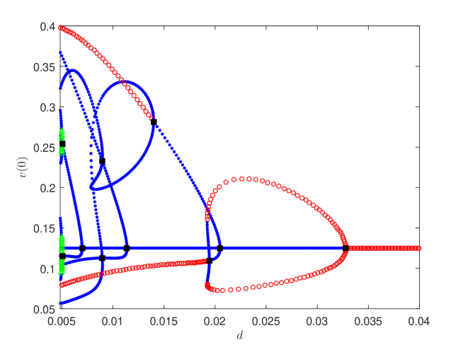
Figure 3: Validated bifurcation diagram of solutions of (4). The space domain $\Omega$ is $(0,1)$, $r_{1}=5$, $r_{2}=2$, $a_{1}=3$, $a_{2}=3$, $b_{1}=1$, $b_{2}=1$, $d_{12}=3$, and $d_{1}=d_{2}=d$ is left as the bifurcation parameter. Each blue dot represents a proved solution, for which we also proved instability. Each green triangle represents a proved solution, that seems unstable numerically but for which we were not able to prove instability. Each red circle represents a proved solution, that seems stable numerically.

Theorem 1.2.

Referring to Figure 3, each blue bullet represents an unstable steady state. Out of the 13 solutions at parameter value $d=0.005$, at least 11 are unstable.

The steady states marked in red in Figure 3 and in particular the two solutions out of 13 that are not concerned by the above Theorem seem to be stable. However, at the moment we are not yet able to use our validation method to prove linear stability, as this requires to control the whole spectrum and not just a single eigenvalue. Still, we point out that the straight line of solutions at $v(0)=0.125$ corresponds to the homogeneous steady state (3), for which the linear stability could of course be studied analytically. In particular it could be proven that, before the bifurcation occuring at $d\simeq 0.0328$ the homogeneous steady state is linearly stable. Validated numerics techniques were used successfully to prove stability in other situations ([11, 29], see also [41]), but the adaptation to our problem presents several challenges (mainly due to the cross-diffusion terms, which muddle the asymptotic structure of the eigenvalue problem, see Section 6) and will be the object of future investigations.

The paper is organized as follows. In Section 2, we give a brief exposition of the validated numerics techniques we apply in this work, as well as additional references on the subject. In particular we state the Theorem 2.1, that serves as common reference and guideline for both the rigorous computation of the steady states and the rigorous enclosure of the eigenvalues. Section 3 is devoted to the introduction of some notations and elementary estimates that are used throughout the paper. In Sections 4 to 5, we then prove the existence of steady states. More precisely, in Section 4.1 we expose how to reformulate the problem of existence of solutions of (4) into a framework suitable for Theorem 2.1. In Section 4.3, we then derive explicit and implementable formulas for the bounds involved in Theorem 2.1, and finally give examples of results in Section 5. Sections 6 to 7 are dedicated to proving the instability of some of these steady states, following the same procedure: suitable reformulation in Section 6.1, bounds in Section 6.3 and results in Section 7.

2 Overview of the rigorous computational method

In this section we briefly explain the strategy for both solving (4) and computing the linear stability of the steady states by means of validated numerics techniques. Each problem is formulated as solving an equation $F(X)=0$ defined on a suitable Banach space. The core of the method, first presented in [49], consists in the introduction of an operator $T$ whose fixed points are in one-to-one correspondence with the zeros of $F(X)$. The existence and enclosure of the solution follow by the Banach fixed point theorem once the operator $T$ is proven to be a contraction on some complete set. The explicit determination of the neighborhood on which the operator is a contraction is done efficiently using the radii polynomial approach (see [18]), which is reminiscent of the Newton-Kantorovich Theorem. The technique can be summarized in the following statement.

Theorem 2.1.

Let $(\mathcal{X},\left\|\cdot\right\|_{\mathcal{X}})$, $(\mathcal{Y},\left\|\cdot\right\|_{\mathcal{Y}})$ be Banach spaces and $F:\mathcal{X}\to\mathcal{Y}$ a $\mathcal{C}^{1}$ function. Let $A:\mathcal{Y}\to\mathcal{X}$ and $A^{{\dagger}}:\mathcal{X}\to\mathcal{Y}$ be linear operators, so that $AF$ maps $\mathcal{X}$ into itself. Let $\bar{X}\in\mathcal{X}$ and assume there exist positive constants $Y$, $Z_{0}$, $Z_{1}$ and a positive function $r\mapsto Z_{2}(r)$ such that

$$\left\|AF(\bar{X})\right\|_{\mathcal{X}} \leq Y$$ (5)

$$\left\VERT I-AA^{{\dagger}}\right\VERT_{\mathcal{X}} \leq Z_{0}$$ (6)

$$\left\VERT A\left(DF(\bar{X})-A^{{\dagger}}\right)\right\VERT_{\mathcal{X}} \leq Z_{1}$$ (7)

$$\left\VERT A\left(DF(X)-DF(\bar{X})\right)\right\VERT_{\mathcal{X}} \leq rZ_{2}(r)\quad\forall~{}X\in\mathcal{B}_{\mathcal{X}}(\bar{X},r),$$ (8)

where $\mathcal{B}_{\mathcal{X}}(\bar{X},r)$ is the closed ball of $\mathcal{X}$, centered at $\bar{X}$ and of radius $r$, and $\VERT\cdot\VERT_{\mathcal{X}}$ denotes the operator norm on $\mathcal{X}$. Define the function $P$ as

$$P(r)=Z_{2}(r)r^{2}-\left(1-(Z_{0}+Z_{1})\right)r+Y.$$ (9)

If there exists $r>0$ such that $P(r)<0$, then the operator $T:\mathcal{X}\to\mathcal{X}$ defined as

$$T=I-AF$$ (10)

has a unique fixed point in $\mathcal{B}_{\mathcal{X}}(\bar{X},r)$. Moreover if $A$ is injective, then $F$ has a unique zero in $\mathcal{B}_{\mathcal{X}}(\bar{X},r)$.

We omit the proof of the theorem, that can be found for instance in [18]. Nevertheless, in the next remark we explain the role of the different operators involved in the theorem and some instructions on how to define them. These considerations are detailed and made more explicit in Section 4.3 (resp. Section 6.3), where we derive the bounds $Y$, $Z_{0}$, $Z_{1}$ and $Z_{2}(r)$ for an $F$ associated to the existence of solutions of (4) (resp. their instability). We also mention that in practice, because of the way we define $A$, its injectivity is in fact implied by the existence of a $r>0$ such that $P(r)<0$ (see Proposition 4.5).

Remark 2.2.

• $\bar{X}$ is chosen as an approximate solution for $F(X)=0$, to be computed numerically as zero for a finite dimensional approximation of $F$. The constant $Y$ is the defect bound and measures how far is $\bar{X}$ from being a fixed point of $T$. Depending on the accuracy of the approximate solution $\bar{X}$, we expect $Y$ to be small.

• The $Z_{i}(r)$, $i=0,1,2$, are meant as bounds for the rate of contraction of the operator $T$ in the ball $\mathcal{B}_{\mathcal{X}}(\bar{X},r)$. More precisely, $Z_{0}+Z_{1}$ provides a bound for the derivative of $T$ at $\bar{X}$, while $Z_{2}(r)$ gives a correction for the derivative in the whole ball $\mathcal{B}_{\mathcal{X}}(\bar{X},r)$. Assume for a moment that $Z_{2}$ is constant. Necessary and sufficient conditions for the existence of an $r>0$ such that $P(r)<0$ are given by

  $$Z_{0}+Z_{1}<1\quad\text{and}\quad\left(1-(Z_{0}+Z_{1})\right)^{2}>4Z_{2}Y.$$

  The two conditions imply that $T$ is a contraction on the ball $\mathcal{B}_{\mathcal{X}}(\bar{X},r)$. In order to obtain a small $Z_{1}$, the operator $A^{{\dagger}}$ is conceived as an approximation of $DF(\bar{X})$ (again based on a finite dimensional approximation of $F$). Similarly, the operator $A$ is constructed as an approximate inverse of $A^{{\dagger}}$, which will then make $Z_{0}$ small. A key point is to define $A^{{\dagger}}$ and $A$ in a smart way, to have good enough approximations while being able to derive tight bounds for $Z_{1}$. Typically $\mathcal{Y}$ is a space of functions less regular than $\mathcal{X}$. To this extent, the operator $A$ acts as a smoothing operator.

• If the nonlinearity of $F$ is a polynomial (say of degree $d$), $Z_{2}$ can be constructed as a polynomial (of degree $d-2$), and therefore $P(r)$ is indeed a polynomial (of same degree $d$ as $F$).

• All the bounds are obtained through a combination of analytic estimates (because the spaces involved are naturally infinite dimensional) and numerical computations (since they depend on the approximate solution $\bar{X}$). To ensure that all possible round off errors are controlled during the computations, we use an interval arithmetic package (in our case INTLAB [45]).

As said in the Introduction, this work is far from being the first application of this kind of rigorous computational techniques to solve systems of PDEs, see for instance [5, 13, 16, 18, 22, 23]. Particularly related to our work is the result presented in [10]. In that paper a similar method was used to rigorously validate a bifurcation diagram of steady states of a 3-component reaction diffusion system (without cross-diffusion term). The system considered in [10] depends on a parameter $\varepsilon$ and it has the property that its steady states approach the solutions of (4) as $\varepsilon$ goes to $0$, see  [27]. However, the proof could only be made for a fixed (small) $\varepsilon$ and the limit case $\varepsilon=0$ is in some sense singular. Therefore the cross-diffusion case could not be handled.

More broadly, techniques similar to the one presented in this work were developed to prove the existence of fixed points, periodic orbits, invariant manifolds and connecting orbits for ordinary differential equations, infinite dimensional maps, partial differential equations and delay differential equations (see for instance [6, 7, 8, 14, 15, 2, 24, 32, 34]). We also mention the existence of comparable techniques where, instead of computing $A$ by using a finite dimensional truncation as we do, a bound on the norm of the inverse of $DF(\bar{X})$ is obtained via spectral estimations (see [44, 37] and the references therein). Instead of the contraction mapping principle, computer assisted proofs in dynamical systems are frequently based on topological tools as covering relations, the Brouwer degree, the fixed point index, the Conley index, see for instance [12, 25, 42, 43, 50]. To conclude this paragraph, we refer the interested reader to [3, 4, 21, 48] for a list, surely not exhaustive, of rigorous computational techniques developed to solve a variety of problems, not necessarily in the area of dynamical systems.

Theorem 2.1 is the cornerstone for all the proofs that are presented in this paper. Whatever problem we want to solve, once the system is rephrased as a zero finding problem and the hypothesis of the theorem are verified, then the proof follows as application of the theorem. Thus, for a given problem $(\mathcal{P})$, we proceed as follows:

1. Introduce a Banach space $(\mathcal{X},\left\|\cdot\right\|_{\mathcal{X}})$ and a $\mathcal{C}^{1}$ function $F$ defined on $\mathcal{X}$ so that the solutions of $F(X)=0$ correspond to solutions of $(\mathcal{P})$;

2. Compute a numerical approximation $\bar{X}\in\mathcal{X}$ so that $F(\bar{X})\approx 0$ and define the linear operators $A$ and $A^{\dagger}$;

3. Define and compute the bounds $Y,Z_{i}(r)$ satisfying (5)-(8);

4. Check that $P(r)$ given in (9) is negative for some $r>0$.

If the last condition is met, the existence of a solution $X$ for $F(X)=0$ is proved in the form specified in the theorem.

In the sequel we detail each step of the above list for the problem of proving existence of steady states (Section 4) and for the problem of proving their linear instability (Section 6).

3 Sequence space, convolutions and norm estimates

The solutions of system (4) as well as the eigenfunctions of the linearised system are sought in the form of Fourier series, which is fairly natural given the boundary conditions included in (4). This approach also provides a very convenient setting to apply our validated numerics technique. In this section we introduce the sequences space relevant for our analysis and we recall some useful properties. The material presented here is standard and mainly included for the sake of completeness and to fix some notations.

Definition 3.1.

Let $\nu>1$. For any sequence $u=\left(u_{k}\right)_{k\geq 0}\in\mathbb{C}^{\mathbb{N}}$ we define the $\nu$-norm of $u$ as

$$\left\|u\right\|_{\nu}=|u_{0}|+2\sum_{k\geq 1}\left|u_{k}\right|\nu^{|k|},$$

and introduce the space

$$\ell^{1}_{\nu}=\left\{u\in\mathbb{C}^{\mathbb{N}},\ \left\|u\right\|_{\nu}<\infty\right\}.$$

We also define $\ell^{1}_{\nu}(\mathbb{R})$ the subspace of $\ell^{1}_{\nu}$ made of real sequences.

Definition 3.2.

For any $u,v\in\ell^{1}_{\nu}$, we define the sequences $(u\ast v)$, $(u\star v)$ and $(u\bullet v)$ as

$$(u\ast v)_{k}=\sum_{\begin{subarray}{c}k_{1},k_{2}\in\mathbb{Z}\\ k_{1}+k_{2}=k\end{subarray}}u_{|k_{1}|}v_{|k_{2}|},\quad(u\star v)_{k}=\sum_{\begin{subarray}{c}k_{1},k_{2}\in\mathbb{Z}\\ k_{1}+k_{2}=k\end{subarray}}\operatorname{sgn}(k_{1})u_{|k_{1}|}v_{|k_{2}|},$$

$$(u\bullet v)_{k}=\sum_{\begin{subarray}{c}k_{1},k_{2}\in\mathbb{Z}\\ k_{1}+k_{2}=k\end{subarray}}\operatorname{sgn}(k_{1})\operatorname{sgn}(k_{2})u_{|k_{1}|}v_{|k_{2}|},$$

where $\operatorname{sgn}(k)$ denotes the sign of $k$ and $\operatorname{sgn}(0)=0$.

The reason for introducing three different convolution products is that we will deal with multiplications of both even and odd functions. The role played by each of the above operations is as follows.

Let $u$ and $v$ in $\ell^{1}_{\nu}$ and consider the even functions (still denoted $u$ and $v$) defined by

$$u(x)=u_{0}+2\sum_{k\geq 1}u_{k}\cos(kx),\quad v(x)=v_{0}+2\sum_{k\geq 1}v_{k}\cos(kx),$$

then $(u\ast v)$ is the sequence of Fourier coefficients of the product function $uv$, i.e.

$$u(x)v(x)=(u\ast v)_{0}+2\sum_{k\geq 1}(u\ast v)_{k}\cos(kx).$$

If instead, $u$ is the odd function given by

$$u(x)=2\sum_{k\geq 1}u_{k}\sin(kx),$$

then $(u\star v)$ provides the sequence of Fourier coefficients of the product function $uv$, i.e.

$$u(x)v(x)=2\sum_{k\geq 1}(u\star v)_{k}\sin(kx).$$

Finally, if both the functions $u$ and $v$ are odd

$$u(x)=2\sum_{k\geq 1}u_{k}\sin(kx),\quad v(x)=2\sum_{k\geq 1}v_{k}\sin(kx),$$

then $(u\bullet v)$ is the sequence of Fourier coefficients of the product function $uv$, i.e.

$$u(x)v(x)=(u\bullet v)_{0}+2\sum_{k\geq 1}(u\bullet v)_{k}\cos(kx).$$

We also recall that $\ell^{1}_{\nu}$ equipped with any of the three convolution products $\ast$, $\star$ or $\bullet$ is a Banach algebra. More precisely we have the following estimate.

Lemma 3.3.

Let $u,v\in\ell^{1}_{\nu}$ and $\circ\in\{\ast,\star,\bullet\}$ any of the convolution products. Then

$$\left\|u\circ v\right\|_{\nu}\leq\left\|u\right\|_{\nu}\left\|v\right\|_{\nu}.$$

Consider now $B:\ell^{1}_{\nu}\to\ell^{1}_{\nu}$ a bounded linear operator. To the operator $B$ is associated a infinite dimensional matrix (still denoted by $B$) so that $(Bu)_{k}=\sum_{j\geq 0}B(k,j)u_{j}$ for all $u$ in $\ell^{1}_{\nu}$. We denote by $\left\VERT B\right\VERT_{\nu}$ the operator norm of $B$, i.e.

$$\left\VERT B\right\VERT_{\nu}=\sup_{\left\|u\right\|_{\nu}=1}\left\|Bu\right\|_{\nu}.$$ (11)

Lemma 3.4.

Let $B:\ell^{1}_{\nu}\to\ell^{1}_{\nu}$ be a linear operator and consider $B(k,j)$ the matrix representation. Then

$$\left\VERT B\right\VERT_{\nu}=\sup_{j\geq 0}\frac{1}{\nu^{j}}\sum_{k\geq 0}|B(k,j)|\nu^{k}.$$

A linear functional $b:\ell^{1}_{\nu}\to\mathbb{R}$ is a particular case of the general operator $B$ given above, when $(B(v))_{k}=0$ for any $k\neq 0$. The linear functional $b$ acts on $u$ as $bu=\sum_{j\geq 0}b_{j}u_{j}$ and the operator norm of $b$ is then given by , $\left\VERT b\right\VERT_{\nu}=\sup_{j\geq 0}\frac{|b(j)|}{\nu^{|j|}}$. We point out that this last formula is linked to the fact that the dual space of $\ell^{1}$ with weight $\nu$ is isometric to the space $\ell^{\infty}$ with weight $\nu^{-1}$.

When dealing with numerical computations, we need to consider only a finite number of coefficients $u_{k}$ in the infinite sequence $u\in\ell^{1}_{\nu}$, that is we consider a finite dimensional projection of $u$.

Definition 3.5.

Let $u\in\ell^{1}_{\nu}$. For $m\in\mathbb{N}$ we denote $\hat{u}^{m}$ the truncated part (i.e. the finite $m$-dimensional projection) of $u$ and $\check{u}^{m}$ the tail part (i.e. infinite dimensional complement) of $u$, given as

$$\hat{u}^{m}_{k}=\left\{\begin{aligned} &u_{k},&k<m,\\ &0,&k\geq m,\end{aligned}\right.\quad\text{and}\quad\check{u}^{m}_{k}=\left\{\begin{aligned} &0,&k<m,\\ &u_{k},&k\geq m.\end{aligned}\right.$$

By a slight abuse of notation, we also refer to $\hat{u}^{m}$ as the finite dimensional vector $\left(u_{k}\right)_{0\leq k<m}$. Moreover, when there is no possible confusion about the dimension of the projection we may drop the exponent $m$ and simply use $\hat{u}$ and $\check{u}$.

We end this section with an estimate used to bound a convolution with a tail term.

Lemma 3.6.

Let $m\in\mathbb{N}$ and $u,v\in\ell^{1}_{\nu}$ and $\circ\in\{\ast,\star,\bullet\}$ any of the convolution products. Then, for all $k\geq 0$,

$$|u\circ\check{v}^{m}|_{k}\leq\Phi^{m}_{k}(u,\nu)\left\|v\right\|_{\nu},$$

where

$$\Phi^{m}_{k}(u,\nu)=\sup\limits_{|l|\geq m}\frac{\left|u_{|l-k|}\right|}{\nu^{|l|}}.$$

4 Framework for the existence of steady states

We are now concerned with the proof of existence of non homogeneous solutions of system (4). According to the algorithm outlined in Section 2, the first step is to reformulate the problem in the form $F(X)=0$, where $F$ is defined on a proper Banach space. Then we introduce the linear operators $A$ and $A^{\dagger}$, and finally we provide the definition of the bounds $Y,Z_{0},Z_{1},Z_{2}(r)$. The latter are then combined to define the radii polynomial $P(r)$.

4.1 Existence of steady states: the function $\bm{F}$

We preventively need to transform (4) into an equivalent system that is more amenable to the application of validated numerics techniques. We introduce further unknown functions and change of coordinates in order to remove the cross-diffusion nonlinearity and to obtain a system with only polynomial nonlinearities (which will be useful when deriving the validation estimates). Then we discretize the obtained system by using Fourier series and finally we introduce $F$ and the Banach space $\mathcal{X}$ in which we look for the solutions.

4.1.1 Auxiliary functions and polynomial system

In order to remove the cross-diffusion nonlinearity we introduce the function $w$ defined as

$$w=(d_{1}+d_{12}v)u.$$

Expressing (4) in term of the unknowns $v$ and $w$ gives simpler higher order terms, but the nonlinear terms become rational functions. To keep the nonlinearity in the form of polynomials, define the function $p$ as

$$p=\frac{1}{d_{1}+d_{12}v},$$ (12)

so that $u=pw$. In term of $w,v,p$, the system (4) takes the form

$$\left\{\begin{aligned} &w^{\prime\prime}+(r_{1}-a_{1}pw-b_{1}v)pw=0,\quad&\text{on }(0,1),\\ &d_{2}v^{\prime\prime}+(r_{2}-b_{2}pw-a_{2}v)v=0,\quad&\text{on }(0,1),\\ &v^{\prime}(0)=v^{\prime}(1)=0,\\ &w^{\prime}(0)=w^{\prime}(1)=0\end{aligned}\right.$$

with $p$ given above as a function of $v(x)$. However, we want to also treat $p$ as an independent unknown, on the same footing as $w$ and $v$. For this, it is enough to append a differential equation and some initial conditions uniquely satisfied by the requested function $p(x)$. Let us consider the equation

$$p^{\prime}=-d_{12}p^{2}v^{\prime},$$

together with the constraint

$$p(0)(d_{1}+d_{12}v(0))=1.$$

It is straightforward to check that the function $p(x)$ in (12) is the only solution of such initial value problem. Finally, introducing a variable $s$ for $v^{\prime}$, we obtain the system

$$\left\{\begin{aligned} &w^{\prime\prime}+(r_{1}-a_{1}pw-b_{1}v)pw=0,\quad&\text{on }(0,1),\\ &d_{2}s^{\prime}+(r_{2}-b_{2}pw-a_{2}v)v=0,\quad&\text{on }(0,1),\\ &p^{\prime}+d_{12}sp^{2}=0,\quad&\text{on }(0,1),\\ &v^{\prime}-s=0,\quad&\text{on }(0,1),\\ &p(0)(d_{1}+d_{12}v(0))=1,\\ &v^{\prime}(0)=v^{\prime}(1)=0,\\ &w^{\prime}(0)=w^{\prime}(1)=0.\end{aligned}\right.$$ (13)

to be solved in the unknowns $w,v,p,s$. We point out that the usage of the variable $p$ to recover polynomial nonlinearities is inspired from [33], where this technique was introduced in the context of validated numerics.

4.1.2 Algebraic system in Fourier space

We now expand the unknown functions and we project the differential system (13) onto the Fourier basis. Because of the boundary conditions and (12), $v(x)$, $w(x)$ and $p(x)$ are written as cosine series. On the opposite, since $s(x)=v^{\prime}(x)$, the function $s(x)$ is expanded on the sines basis. Precisely, consider

$$\begin{array}[]{ll}{\displaystyle w(x)=w_{0}+2\sum_{k\geq 1}w_{k}\cos(k\pi x),}&{\displaystyle v(x)=v_{0}+2\sum_{k\geq 1}v_{k}\cos(k\pi x),}\\ {\displaystyle p(x)=p_{0}+2\sum_{k\geq 1}p_{k}\cos(k\pi x),}&{\displaystyle s(x)=s_{0}+2\sum_{k\geq 1}s_{k}\sin{(k\pi x)}.}\end{array}$$ (14)

The addition of the $s_{0}$ coefficient (which is clearly zero since $s=v^{\prime}$) is deliberate, because we see each of the sequence of Fourier coefficients $\left(v_{k}\right)_{k\geq 0}$, $\left(w_{k}\right)_{k\geq 0}$, $\left(p_{k}\right)_{k\geq 0}$ and $\left(s_{k}\right)_{k\geq 0}$ as an element of $\ell^{1}_{\nu}$. Plugging these series expansions into (13) and then projecting back onto the cosine/sine basis, we obtain the following (infinite dimensional) algebraic system

$$\left\{\begin{aligned} &-(\pi k)^{2}w_{k}+r_{1}(p\ast w)_{k}-a_{1}(p\ast p\ast w\ast w)_{k}-b_{1}(p\ast v\ast w)_{k}=0,\quad&\forall~{}k\in\mathbb{N},\\ &d_{2}\pi ks_{k}+r_{2}v_{k}-a_{2}(v\ast v)_{k}-b_{2}(p\ast v\ast w)_{k}=0,\quad&\forall~{}k\in\mathbb{N},\\ &-\pi kp_{k}+d_{12}(s\star p\ast p)_{k}=0,\quad&\forall~{}k\in\mathbb{N},\\ &-\pi kv_{k}-s_{k}=0,\quad&\forall~{}k\in\mathbb{N},\\ &\left(p_{0}+2\sum_{k\geq 1}p_{k}\right)\left(d_{1}+d_{12}\left(v_{0}+2\sum_{k\geq 1}v_{k}\right)\right)-1=0.\end{aligned}\right.$$ (15)

to be solved for the unknown sequences $w=\{w_{k}\}_{k\geq 0},v=\{v_{k}\}_{k\geq 0},p=\{p_{k}\}_{k\geq 0},s=\{s_{k}\}_{k\geq 0}$.

Notice that because of the equation $-\pi kv_{k}-s_{k}=0$ with $k=0$, any solution of this system does indeed satisfy $s_{0}=0$. Notice also that for $k=0$, the equation $-\pi kp_{k}+d_{12}(s\star p\ast p)_{k}=0$ is an identity. Indeed $-0\pi p_{0}=0$, and it follows from the definition of the convolution products $\star$ that $(s\star p\ast p)_{0}=0$. In other words, since $p(x)$ is even and $s(x)$ is odd, the product $sp^{2}$ is odd, hence the $0$-th Fourier coefficients vanishes. Therefore this equation can be removed and we are then left with a square system.

4.1.3 The $\bm{F=0}$ formulation

For $\nu>1$, we define $\mathcal{X}_{\nu}=\left(\ell^{1}_{\nu}(\mathbb{R})\right)^{4}$, where $\ell^{1}_{\nu}$ is given in Definition 3.1, and denote by $X=(v,w,p,s)$ any element in $\mathcal{X}_{\nu}$. We also use the notation $X_{k}$ to denote $(v_{k},w_{k},p_{k},s_{k})$. We endow $\mathcal{X}_{\nu}$ with the norm

$$\left\|X\right\|_{\mathcal{X}_{\nu}}=\left\|v\right\|_{\nu}+\left\|w\right\|_{\nu}+\left\|p\right\|_{\nu}+\left\|s\right\|_{\nu},$$ (16)

which makes it a Banach space. We then define the function $F=(F^{(v)},F^{(w)},F^{(p)},F^{(s)})$ acting on $\mathcal{X}_{\nu}$ by

$$F_{k}^{(v)}(X)=-\pi kv_{k}-s_{k},\quad \forall~{}k\in\mathbb{N},$$ (17)

$$F_{k}^{(w)}(X)=-(\pi k)^{2}w_{k}+r_{1}(p\ast w)_{k}-a_{1}(p\ast p\ast w\ast w)_{k}-b_{1}(p\ast v\ast w)_{,}\quad \forall~{}k\in\mathbb{N},$$ (18)

$$F_{0}^{(p)}(X)=\left(p_{0}+2\sum_{k\geq 1}p_{k}\right)\left(d_{1}+d_{12}\left(v_{0}+2\sum_{k\geq 1}v_{k}\right)\right)-1,$$ (19)

$$F_{k}^{(p)}(X)=-\pi kp_{k}+d_{12}(s\star p\ast p)_{k},\quad \forall~{}k\geq 1,$$ (20)

$$F_{k}^{(s)}(X)=d_{2}\pi ks_{k}+r_{2}v_{k}-a_{2}(v\ast v)_{k}-b_{2}(p\ast v\ast w)_{k},\quad \forall~{}k\in\mathbb{N}.$$ (21)

The next Lemma summarizes and justifies in a precise statement all the formal computations and substitutions made previously in this section, with the goal of solving system (4).

Lemma 4.1.

Let $\nu>1$. Assume that there exists $X\in\mathcal{X}_{\nu}$ such that $F(X)=0$ and consider as in (14) the functions $v$, $w$, $p$ and $s$. Assume also that the coefficients $\left(v_{k}\right)_{k\geq 0}$ and $\left(w_{k}\right)_{k\geq 0}$ are such that the functions $v$ and $w$ are positive. Define the function $u=pw$. Then $u$ and $v$ are smooth positive functions that solve (4).

Proof.

First notice that since $X\in\mathcal{X}_{\nu}$ with $\nu>1$, the Fourier coefficients are decaying exponentially fast to 0, and thus the functions $v$, $w$, $p$ and $s$ are well defined and smooth (in fact analytic) $2$-periodic functions. Then, having $F(X)=0$ means exactly that the sequences $\left(v_{k}\right)_{k\geq 0}$, $\left(w_{k}\right)_{k\geq 0}$, $\left(p_{k}\right)_{k\geq 0}$ and $\left(s_{k}\right)_{k\geq 0}$ solve (15), which in turn implies that the functions $v$, $w$, $p$ and $s$ solve (13). All the derivatives needed in (13) are legitimate thanks to the exponential decay of the coefficients. Besides, since $p$ satisfies the differential equation $p^{\prime}+d_{12}p^{2}v^{\prime}=0$ and $p(0)(d_{1}+d_{12}v(0))=1$, by uniqueness we have

$$p=\frac{1}{d_{1}+d_{12}v}.$$

Therefore $w=\frac{u}{p}=(d_{1}+d_{12}v)u$ and $(u,v)$ does indeed solve (4) (the boundary condition for $u$ is also satisfied since $u^{\prime}(0)=p^{\prime}(0)w(0)+p(0)w^{\prime}(0)=0$ and $u^{\prime}(1)=p^{\prime}(1)w(1)+p(1)w^{\prime}(1)=0$). ∎

4.2 Existence of steady states: the operators $\bm{A}$ and $\bm{A^{\dagger}}$

As outlined in Remark (2.2), the definition of the operators $A$ and $A^{\dagger}$ is based on some approximate solution $\bar{X}$, which is computed as numerical zero of a finite dimensional projection of $F(X)=0$.

Extending the notations introduced in Definition 3.5, for $X\in\mathcal{X}_{\nu}$ we denote $\hat{X}^{m}$ the vector of truncated sequences, i.e.

$$\hat{X}^{m}=(\hat{v}^{m},\hat{w}^{m},\hat{p}^{m},\hat{s}^{m}).$$

Similarly,

$$\hat{F}^{m}=\left(\left(F^{(v)}_{k}\right)_{0\leq k<m},\left(F^{(w)}_{k}\right)_{0\leq k<m},\left(F^{(p)}_{k}\right)_{0\leq k<m},\left(F^{(s)}_{k}\right)_{0\leq k<m}\right).$$

We consider $\hat{F}^{m}$ as acting on truncated sequences $\hat{X}^{m}$ only, so that we can see it as a function mapping $\mathbb{R}^{4m}$ to itself. Therefore, finding $\hat{X}^{m}$ such that $\hat{F}^{m}(\hat{X}^{m})=0$ is a finite dimensional problem that can be solved numerically. We now assume to have computed numerically a zero of $\hat{F}^{m}$, denoted by $\bar{X}$.

The linear operator $A^{{\dagger}}$ is defined as an approximation of $DF(\bar{X})$. However, since we will also need to construct an approximate inverse of $A^{{\dagger}}$, $A^{{\dagger}}$ is required to have a simple structure. In practice we impose that $A^{\dagger}$ acts diagonally on the tail $\{X_{k}\}_{k\geq m}$. More precisely, we define $A^{{\dagger}}$ (acting on $X=(v,w,p,s)\in\mathcal{X}_{\nu}$), as

$$\widehat{A^{{\dagger}}X}^{m}=D\hat{F}^{m}(\bar{X})\hat{X}^{m},$$ (22)

and

$$\left(A^{{\dagger}}X\right)_{k}=\left(-\pi kv_{k},-(\pi k)^{2}w_{k},-\pi kp_{k},d_{2}\pi ks_{k}\right),\quad\forall~{}k\geq m.$$

The operator $A$ is then constructed as an approximate inverse of $A^{{\dagger}}$. We consider $\hat{A}^{m}$ a numerically computed inverse of $D\hat{F}^{m}(\bar{X})$ and define $A$ (acting on $X=(v,w,p,s)\in\mathcal{X}_{\nu}$), as

$$\widehat{AX}^{m}=\hat{A}^{m}\hat{X}^{m},$$

and

$$\left(AX\right)_{k}=\left(-(\pi k)^{-1}v_{k},-(\pi k)^{-2}w_{k},-(\pi k)^{-1}p_{k},(d_{2}\pi k)^{-1}s_{k}\right),\quad\forall~{}k\geq m.$$

The definition of $A$ and the fact that $\ell^{1}_{\nu}$ is a algebra for both convolution products $\ast$ and $\star$ (see Lemma 3.3) ensure that $AF$ does map $\mathcal{X}_{\nu}$ into itself, as requested in the hypothesis of Theorem 2.1.

Remark 4.2.

To define the action of $A^{{\dagger}}$ on the tail space, we simply kept the asymptotically dominant terms of the derivative $DF(\bar{X})$. Since these terms act diagonally, we are able to easily and analytically invert the tail of $A^{{\dagger}}$ and hence to define $A$. However, the fact that the dominant terms of the derivative are diagonal is not a mere happenstance, rather it is the result of the various reformulations performed in Section 4.1.1. Had we not introduced the function $w$, the Fourier expansion of the cross-diffusion term would create a messy dominant expression that we would not be able to invert analytically.

4.3 Existence of steady states: the bounds $\bm{Y}$ and $\bm{Z_{i}(r)}$

Having the Banach space $\mathcal{X}_{\nu}$, the function $F$, the approximate solution $\bar{X}=(\bar{v},\bar{w},\bar{p},\bar{s})$ and the operators $A$, $A^{{\dagger}}$ in hands, we now proceed to derive computable bounds $Y$, $Z_{0}$, $Z_{1}$ and $Z_{2}$ satisfying (5)-(8) (for $\mathcal{X}=\mathcal{X}_{\nu}$).

4.3.1 The bound $\bm{Y}$

The definition of the bound $Y$ is rather straightforward, and we just consider

$$Y=\left\|AF(\bar{X})\right\|_{\mathcal{X}_{\nu}}.$$ (23)

The key observation here is that $Y$ can be computed explicitly. Indeed, we recall that $\bar{X}\in\hat{X}^{m}$ is a truncated sequence, i.e. $\bar{X}_{k}=(\bar{v}_{k},\bar{w}_{k},\bar{p}_{k},\bar{s}_{k})=(0,0,0,0)$ for all $k\geq m$. Therefore we have

$$F_{k}^{(v)}(\bar{X})=0,\quad\forall~{}k\geq m,\qquad F_{k}^{(w)}(\bar{X})=0,\quad\forall~{}k\geq 4m-3,$$

$$F_{k}^{(p)}(\bar{X})=0,\quad\forall~{}k\geq 3m-2,\qquad F_{k}^{(s)}(\bar{X})=0,\quad\forall~{}k\geq 3m-2,$$

and thus $F(\bar{X})$ only has a finite number of non zero coefficients. This is also true for $AF(\bar{X})$ (thanks to the diagonal structure of the tail of $A$), and therefore $\left\|AF(\bar{X})\right\|_{\mathcal{X}_{\nu}}$ can be evaluated on a computer. To be completely precise, what we mean by (23) is that a (sharp) upper bound of $\left\|AF(\bar{X})\right\|_{\mathcal{X}_{\nu}}$ can be computed using interval arithmetic, and that we define $Y$ to be this upper bound. We are going to repeat this abuse of language whenever we define bounds that involve terms that have to be evaluated on a computer.

4.3.2 The bound $\bm{Z_{0}}$

In this section we focus on getting a bound $Z_{0}$ satisfying (6). Here and thereafter, when dealing with linear operators on $\mathcal{X}_{\nu}$, it is convenient to use a block notation. For a linear operator $B:\mathcal{X}_{\nu}\to\mathcal{X}_{\nu}$, we consider the decomposition

$$B=\begin{pmatrix}B^{(v,v)}&B^{(v,w)}&B^{(v,p)}&B^{(v,s)}\\ B^{(w,v)}&B^{(w,w)}&B^{(w,p)}&B^{(w,s)}\\ B^{(p,v)}&B^{(p,w)}&B^{(p,p)}&B^{(p,s)}\\ B^{(s,v)}&B^{(s,w)}&B^{(s,p)}&B^{(s,s)}\end{pmatrix},\quad{\rm each}\ B^{(i,j)}:\ell^{1}_{\nu}(\mathbb{R})\to\ell^{1}_{\nu}(\mathbb{R})$$

so that, for $X=(v,w,p,s)\in\mathcal{X}_{\nu}$,

$$\left(BX\right)^{(v)}=B^{(v,v)}v+B^{(v,w)}w+B^{(v,p)}p+B^{(v,s)}s,$$

and similarly for the other components. Thus, recalling (16) and the operator norm (11),

$$\left\|BX\right\|_{\mathcal{X}_{\nu}} =\left\|\left(BX\right)^{(v)}\right\|_{\nu}+\left\|\left(BX\right)^{(w)}\right\|_{\nu}+\left\|\left(BX\right)^{(p)}\right\|_{\nu}+\left\|\left(BX\right)^{(s)}\right\|_{\nu}$$ (24)

$$\leq\Theta_{B}^{(v)}\left\|v\right\|_{\nu}+\Theta_{B}^{(w)}\left\|w\right\|_{\nu}+\Theta_{B}^{(p)}\left\|p\right\|_{\nu}+\Theta_{B}^{(s)}\left\|s\right\|_{\nu}$$ (25)

$$\leq\max\left[\Theta_{B}^{(v)},\Theta_{B}^{(w)},\Theta_{B}^{(p)},\Theta_{B}^{(s)}\right]\left\|X\right\|_{\mathcal{X}_{\nu}},$$ (26)

where

$$\Theta_{B}^{(i)}=\VERT B^{(v,i)}\VERT_{\nu}+\VERT B^{(w,i)}\VERT_{\nu}+\VERT B^{(p,i)}\VERT_{\nu}+\VERT B^{(s,i)}\VERT_{\nu},\quad\forall i\in\{v,w,p,s\}.$$

Therefore, we define

$$Z_{0}=\max\left[\Theta_{I-AA^{{\dagger}}}^{(v)},\Theta_{I-AA^{{\dagger}}}^{(w)},\Theta_{I-AA^{{\dagger}}}^{(p)},\Theta_{I-AA^{{\dagger}}}^{(s)}\right].$$ (27)

Notice that, since the tail part of $A$ and $A^{{\dagger}}$ are exact inverse of each other by definition, the tail part of $I-AA^{{\dagger}}$ is zero. Therefore, each block in the decomposition of $I-AA^{{\dagger}}$ has only finitely many non zero coefficients, and each $\Theta_{I-AA^{{\dagger}}}^{(i)}$ can be computed using Lemma 3.4, the supremum and the sum ranging only over finitely many coefficients.

4.3.3 The bound $\bm{Z_{1}}$

In this section we focus on getting a bound $Z_{1}$ satisfying 7.

Lemma 4.3.

Let $\hat{\alpha}^{m}_{v},\hat{\alpha}^{m}_{w},\hat{\alpha}^{m}_{p},\hat{\alpha}^{m}_{s}$ be vectors in $\mathbb{R}^{4m}$ each, defined as

$$(\hat{\alpha}^{m}_{v})_{0} =\begin{pmatrix}0\\ \Phi_{0}^{m}(-b_{1}(\bar{p}\ast\bar{w}),\nu)\\ \left|d_{12}\left(\bar{p}_{0}+2\sum_{k\geq 1}\bar{p}_{k}\right)\right|\frac{2}{\nu^{m}}\\ \Phi_{0}^{m}(-2a_{2}\bar{v}-b_{2}(\bar{p}\ast\bar{w}),\nu)\end{pmatrix},\quad(\hat{\alpha}^{m}_{w})_{0}=\begin{pmatrix}0\\ \Phi_{0}^{m}(r_{1}\bar{p}-2a_{1}(\bar{p}\ast\bar{p}\ast\bar{w})-b_{1}(\bar{p}\ast\bar{v}),\nu)\\ 0\\ \Phi_{0}^{m}(-b_{2}(\bar{p}\ast\bar{v}),\nu)\end{pmatrix},$$

$$(\hat{\alpha}^{m}_{p})_{0} =\begin{pmatrix}0\\ \Phi_{0}^{m}(r_{1}\bar{w}-2a_{1}(\bar{p}\ast\bar{w}\ast\bar{w})-b_{1}(\bar{v}\ast\bar{w}),\nu)\\ \left|d+d_{12}\left(\bar{v}_{0}+2\sum_{k\geq 1}\bar{v}_{k}\right)\right|\frac{2}{\nu^{m}}\\ \Phi_{0}^{m}(-b_{2}(\bar{v}\ast\bar{w}),\nu)\end{pmatrix},\quad(\hat{\alpha}^{m}_{s})_{0}=\begin{pmatrix}0\\ 0\\ \Phi_{0}^{m}(d_{12}(\bar{p}\ast\bar{p}),\nu)\\ 0\end{pmatrix}$$

and for each $1\leq k<m$,

$$(\hat{\alpha}^{m}_{v})_{k} =\begin{pmatrix}0\\ \Phi_{k}^{m}(-b_{1}(\bar{p}\ast\bar{w}),\nu)\\ 0\\ \Phi_{k}^{m}(-2a_{2}\bar{v}-b_{2}(\bar{p}\ast\bar{w}),\nu)\end{pmatrix},\quad(\hat{\alpha}^{m}_{w})_{k}=\begin{pmatrix}0\\ \Phi_{k}^{m}(r_{1}\bar{p}-2a_{1}(\bar{p}\ast\bar{p}\ast\bar{w})-b_{1}(\bar{p}\ast\bar{v}),\nu)\\ 0\\ \Phi_{k}^{m}(-b_{2}(\bar{p}\ast\bar{v}),\nu)\end{pmatrix}$$

$$(\hat{\alpha}^{m}_{p})_{k} =\begin{pmatrix}0\\ \Phi_{k}^{m}(r_{1}\bar{w}-2a_{1}(\bar{p}\ast\bar{w}\ast\bar{w})-b_{1}(\bar{v}\ast\bar{w}),\nu)\\ \Phi_{k}^{m}(2d_{12}(\bar{s}\star\bar{p}),\nu)\\ \Phi_{k}^{m}(-b_{2}(\bar{v}\ast\bar{w}),\nu)\end{pmatrix},\quad(\hat{\alpha}^{m}_{s})_{k}=\begin{pmatrix}0\\ 0\\ \Phi_{k}^{m}(d_{12}(\bar{p}\ast\bar{p}),\nu)\\ 0\end{pmatrix}.$$

Define

$$Z_{1} =\max\left[\left\||A|\hat{\alpha}^{m}_{v}\right\|_{\mathcal{X}_{\nu}},\left\||A|\hat{\alpha}^{m}_{w}\right\|_{\mathcal{X}_{\nu}},\left\||A|\hat{\alpha}^{m}_{p}\right\|_{\mathcal{X}_{\nu}},\left\||A|\hat{\alpha}^{m}_{s}\right\|_{\mathcal{X}_{\nu}}\right]$$

$$\quad+\max\left[\left(\frac{\left\|b_{1}(\bar{p}\ast\bar{w})\right\|_{\nu}}{(\pi m)^{2}}+\frac{\left\|r_{2}-2a_{2}\bar{v}-b_{2}(\bar{p}\ast\bar{w})\right\|_{\nu}}{d\pi m}\right),\right.$$

$$\qquad\qquad\left(\frac{\left\|r_{1}\bar{p}-2a_{1}(\bar{p}\ast\bar{p}\ast\bar{w})-b_{1}(\bar{p}\ast\bar{v})\right\|_{\nu}}{(\pi m)^{2}}+\frac{\left\|b_{2}(\bar{p}\ast\bar{v})\right\|_{\nu}}{d\pi m}\right),$$

$$\qquad\qquad\left(\frac{\left\|r_{1}\bar{w}-2a_{1}(\bar{p}\ast\bar{w}\ast\bar{w})-b_{1}(\bar{v}\ast\bar{w})\right\|_{\nu}}{(\pi m)^{2}}+\frac{\left\|2d_{12}(\bar{s}\star\bar{p})\right\|_{\nu}}{\pi m}+\frac{\left\|b_{2}(\bar{v}\ast\bar{w})\right\|_{\nu}}{d\pi m}\right),$$

$$\left.\qquad\qquad\left(\frac{1}{\pi m}+\frac{\left\|d_{12}(\bar{p}\ast\bar{p})\right\|_{\nu}}{\pi m}\right)\right].$$ (28)

Then

$$Z_{1}\geq\left\VERT A\left(DF(\bar{X})-A^{{\dagger}}\right)\right\VERT_{\mathcal{X}_{\nu}}.$$

Proof.

According to (7), we need a bound for

$$A\left(DF(\bar{X})-A^{{\dagger}}\right)X,$$

for $X\in B_{\mathcal{X}_{\nu}}(0,1)$. Denoting $U=\left(DF(\bar{X})-A^{{\dagger}}\right)X$ and using the triangular inequality, we have

$$\left\|A\left(DF(\bar{X})-A^{{\dagger}}\right)X\right\|_{\mathcal{X}_{\nu}} \leq\left\||A||U|\right\|_{\mathcal{X}_{\nu}}$$

$$\leq\||A||\hat{U}^{m}|\|_{\mathcal{X}_{\nu}}+\||A||\check{U}^{m}|\|_{\mathcal{X}_{\nu}},$$

where here and in the sequel, the absolute values must be understood component-wise. We point out that, since $A$ is built as a finite dimensional block $\hat{A}^{m}$ (acting on $\hat{U}^{m}$) and a diagonal tail, it follows that $|A||\hat{U}^{m}|=|\hat{A}^{m}||\hat{U}^{m}|$ is a finite vector, (it has non zero components only for $k<m$), whereas $|A||\check{U}^{m}|$ has non zero components only for $k\geq m$. We provide a bound for both terms separately.

At first, let us compute a bound on $|\hat{U}^{m}|$. Recalling from (22) that $A^{\dagger}$ is defined so that

$$\widehat{A^{{\dagger}}X}^{m}=D\hat{F}^{m}(\bar{X})\hat{X}^{m},$$

it follows that in computing $\hat{U}^{m}$ all the linear contributions of $X$ cancel out. Explicitly, using Lemma 3.6, a meticulous though straightforward analysis gives

$$|\hat{U}^{m}|\leq(\hat{\alpha}^{m}_{v})\left\|v\right\|_{\nu}+(\hat{\alpha}^{m}_{w})\left\|w\right\|_{\nu}+(\hat{\alpha}^{m}_{p})\left\|p\right\|_{\nu}+(\hat{\alpha}^{m}_{s})\left\|s\right\|_{\nu}.$$

The vectors $\hat{\alpha}^{m}_{i}$ can each be seen as an element of $\mathbb{R}^{4m}$, or equivalently of $\mathcal{X}_{\nu}$ with coefficients equal to $0$ for all $k\geq m$. Inserting he previous inequality into $|A||\hat{U}^{m}|$, we have that

$$\||A||\hat{U}^{m}|\|_{\mathcal{X}_{\nu}} \leq\left\||A|\hat{\alpha}^{m}_{v}\right\|_{\mathcal{X}_{\nu}}\left\|v\right\|_{\nu}+\left\||A|\hat{\alpha}^{m}_{w}\right\|_{\mathcal{X}_{\nu}}\left\|w\right\|_{\nu}+\left\||A|\hat{\alpha}^{m}_{p}\right\|_{\mathcal{X}_{\nu}}\left\|p\right\|_{\nu}+\left\||A|\hat{\alpha}^{m}_{s}\right\|_{\mathcal{X}_{\nu}}\left\|s\right\|_{\nu}$$

$$\leq\max\left[\left\||A|\hat{\alpha}^{m}_{v}\right\|_{\mathcal{X}_{\nu}},\left\||A|\hat{\alpha}^{m}_{w}\right\|_{\mathcal{X}_{\nu}},\left\||A|\hat{\alpha}^{m}_{p}\right\|_{\mathcal{X}_{\nu}},\left\||A|\hat{\alpha}^{m}_{s}\right\|_{\mathcal{X}_{\nu}}\right]\left\|X\right\|_{\mathcal{X}_{\nu}},$$ (29)

the maximum being taken over terms that can all be evaluated on a computer.

For the tail part (i.e. for modes $k\geq m$), $A^{{\dagger}}$ only cancels the diagonal dominant terms, and we have

$$|U_{k}| \leq\begin{pmatrix}0\\ \left(|b_{1}(\bar{p}\ast\bar{w})|\ast|v|\right)_{k}\\ 0\\ \left(|r_{2}-2a_{2}\bar{v}-b_{2}(\bar{p}\ast\bar{w})|\ast|v|\right)_{k}\end{pmatrix}+\begin{pmatrix}0\\ \left(|r_{1}\bar{p}-2a_{1}(\bar{p}\ast\bar{p}\ast\bar{w})-b_{1}(\bar{p}\ast\bar{v})|\ast|w|\right)_{k}\\ 0\\ \left(|b_{2}(\bar{p}\ast\bar{v})|\ast|w|\right)_{k}\end{pmatrix}$$

$$\quad+\begin{pmatrix}0\\ \left(|r_{1}\bar{w}-2a_{1}(\bar{p}\ast\bar{w}\ast\bar{w})-b_{1}(\bar{v}\ast\bar{w})|\ast|p|\right)_{k}\\ \left(|2\alpha(\bar{s}\star\bar{p})|\ast|p|\right)_{k}\\ \left(|b_{2}(\bar{v}\ast\bar{w})|\ast|p|\right)_{k}\end{pmatrix}+\begin{pmatrix}|s|_{k}\\ 0\\ \left(|d_{12}(\bar{p}\ast\bar{p})|\star|s|\right)_{k}\\ 0\end{pmatrix}.$$

Using Lemma 3.3, and the definition of the tail part of $A$, we get

$$\left\||A||\check{U}^{m}|\right\|_{\mathcal{X}_{\nu}} \leq\left(\frac{\left\|b_{1}(\bar{p}\ast\bar{w})\right\|_{\nu}}{(\pi m)^{2}}+\frac{\left\|r_{2}-2a_{2}\bar{v}-b_{2}(\bar{p}\ast\bar{w})\right\|_{\nu}}{d\pi m}\right)\left\|v\right\|_{\nu}$$

$$\quad+\left(\frac{\left\|r_{1}\bar{p}-2a_{1}(\bar{p}\ast\bar{p}\ast\bar{w})-b_{1}(\bar{p}\ast\bar{v})\right\|_{\nu}}{(\pi m)^{2}}+\frac{\left\|b_{2}(\bar{p}\ast\bar{v})\right\|_{\nu}}{d\pi m}\right)\left\|w\right\|_{\nu}$$

$$\quad+\left(\frac{\left\|r_{1}\bar{w}-2a_{1}(\bar{p}\ast\bar{w}\ast\bar{w})-b_{1}(\bar{v}\ast\bar{w})\right\|_{\nu}}{(\pi m)^{2}}+\frac{\left\|2\alpha(\bar{s}\star\bar{p})\right\|_{\nu}}{\pi m}+\frac{\left\|b_{2}(\bar{v}\ast\bar{w})\right\|_{\nu}}{d\pi m}\right)\left\|p\right\|_{\nu}$$

$$\quad+\left(\frac{1}{\pi m}+\frac{\left\|d_{12}(\bar{p}\ast\bar{p})\right\|_{\nu}}{\pi m}\right)\left\|s\right\|_{\nu}$$

$$\leq\max\left[\left(\frac{\left\|b_{1}(\bar{p}\ast\bar{w})\right\|_{\nu}}{(\pi m)^{2}}+\frac{\left\|r_{2}-2a_{2}\bar{v}-b_{2}(\bar{p}\ast\bar{w})\right\|_{\nu}}{d\pi m}\right),\right.$$

$$\qquad\qquad\left(\frac{\left\|r_{1}\bar{p}-2a_{1}(\bar{p}\ast\bar{p}\ast\bar{w})-b_{1}(\bar{p}\ast\bar{v})\right\|_{\nu}}{(\pi m)^{2}}+\frac{\left\|b_{2}(\bar{p}\ast\bar{v})\right\|_{\nu}}{d\pi m}\right),$$

$$\qquad\qquad\left(\frac{\left\|r_{1}\bar{w}-2a_{1}(\bar{p}\ast\bar{w}\ast\bar{w})-b_{1}(\bar{v}\ast\bar{w})\right\|_{\nu}}{(\pi m)^{2}}+\frac{\left\|2d_{12}(\bar{s}\star\bar{p})\right\|_{\nu}}{\pi m}+\frac{\left\|b_{2}(\bar{v}\ast\bar{w})\right\|_{\nu}}{d\pi m}\right),$$

$$\left.\qquad\qquad\left(\frac{1}{\pi m}+\frac{\left\|d_{12}(\bar{p}\ast\bar{p})\right\|_{\nu}}{\pi m}\right)\right]\left\|X\right\|_{\mathcal{X}_{\nu}}.$$

The sum of the latter estimate and (29) provides the bound $Z_{1}$ (4.3). ∎

It is important to remark that all the $\Phi_{k}^{m}$ functions involved in the definition of $\hat{\alpha}^{m}_{i}$, $i\in\{v,w,p,s\}$, take as arguments sequences that only have a finite number of non zero coefficients and that are given in terms of the numerical guess $\bar{X}$. Therefore, all the vectors of coefficients and the bound $Z_{1}$ can be rigorously and explicitly computed.

4.3.4 The bound $\bm{Z_{2}}$

In this section we focus on defining a bound $Z_{2}$ satisfying (8).

Lemma 4.4.

Consider the block decomposition of $A$ and the associated coefficients $\Theta_{A}$, as introduced in Section 4.3.2. Define the quantities

$$\alpha_{v,v^{\prime}}=2a_{2}\Theta_{A}^{(s)},\quad\alpha_{w,w^{\prime}}=2a_{1}\left\|\bar{p}\ast\bar{p}\right\|_{\nu}\Theta_{A}^{(w)},\quad\alpha_{p,p^{\prime}}=2a_{1}\left\|\bar{w}\ast\bar{w}\right\|_{\nu}\Theta_{A}^{(w)}+2d_{12}\left\|\bar{s}\right\|_{\nu}\Theta_{A}^{(p)},$$

$$\alpha_{v,w^{\prime}}=b_{1}\left\|\bar{p}\right\|_{\nu}\Theta_{A}^{(w)}+b_{2}\left\|\bar{p}\right\|_{\nu}\Theta_{A}^{(s)},\quad\alpha_{v,p^{\prime}}=b_{1}\left\|\bar{w}\right\|_{\nu}\Theta_{A}^{(w)}+d_{12}\Theta_{A}^{(p)}+b_{2}\left\|\bar{w}\right\|_{\nu}\Theta_{A}^{(s)},$$

$$\alpha_{w,p^{\prime}}=\left\|r_{1}-4a_{1}\bar{w}\ast\bar{p}-b_{1}\bar{v}\right\|_{\nu}\Theta_{A}^{(w)}+b_{2}\left\|\bar{v}\right\|_{\nu}\Theta_{A}^{(s)},\quad\alpha_{p,s^{\prime}}=2d_{12}\left\|\bar{p}\right\|_{\nu}\Theta_{A}^{(p)},$$

and

$$\alpha_{v,w^{\prime},p^{\prime\prime}}=b_{1}\Theta_{A}^{(w)}+b_{2}\Theta_{A}^{(s)},\quad\alpha_{w,w^{\prime},p^{\prime\prime}}=4a_{1}\left\|\bar{p}\right\|_{\nu}\Theta_{A}^{(w)},$$

$$\alpha_{w,p^{\prime},p^{\prime\prime}}=4a_{1}\left\|\bar{w}\right\|_{\nu}\Theta_{A}^{(w)},\quad\alpha_{p,p^{\prime},s^{\prime\prime}}=2d_{12}\Theta_{A}^{(p)},$$

and

$$\alpha_{w,,w^{\prime},p^{\prime\prime},p^{\prime\prime\prime}}=4a_{1}\Theta_{A}^{(w)}.$$

Define

$$Z_{2}(r) =\max\left[\alpha_{v,v^{\prime}},\alpha_{w,w^{\prime}},\alpha_{p,p^{\prime}},\alpha_{v,w^{\prime}},\alpha_{v,p^{\prime}},\alpha_{w,p^{\prime}},\alpha_{p,s^{\prime}}\right]$$

$$\quad+\frac{1}{2}\max\left[\alpha_{v,w^{\prime},p^{\prime\prime}},\alpha_{w,w^{\prime},p^{\prime\prime}},\alpha_{w,p^{\prime},p^{\prime\prime}},\alpha_{p,p^{\prime},s^{\prime\prime}}\right]r$$

$$\quad+\frac{1}{6}\alpha_{w,w^{\prime},p^{\prime\prime},p^{\prime\prime\prime}}r^{2}.$$ (30)

Then

$$rZ_{2}(r)\geq\left\VERT A\left(DF(X)-DF(\bar{X})\right)\right\VERT_{\mathcal{X}}\quad\forall~{}X\in\mathcal{B}_{\mathcal{X}}(\bar{X},r).$$

Proof.

Consider the expansion:

$$A\left(DF(\bar{X}+X^{\prime})-DF(\bar{X})\right)X =AD^{2}F(\bar{X})(X^{\prime},X)$$

$$\quad+\frac{1}{2}AD^{3}F(\bar{X})(X^{\prime},X^{\prime},X)$$

$$\quad+\frac{1}{6}AD^{4}F(\bar{X})(X^{\prime},X^{\prime},X^{\prime},X).$$

We provide bounds for each term on the right hand side, uniform for all $X\in B_{\mathcal{X}_{\nu}}(0,1)$ and $X^{\prime}\in B_{\mathcal{X}_{\nu}}(0,r)$.

For the quadratic term, we have that

$$\left\|D^{2}F^{(v)}(\bar{X})(X^{\prime},X)\right\|_{\nu}= \,0,$$

$$\left\|D^{2}F^{(w)}(\bar{X})(X^{\prime},X)\right\|_{\nu}\leq \,b_{1}\left\|\bar{w}\right\|_{\nu}\left(\left\|v\right\|_{\nu}\left\|p^{\prime}\right\|_{\nu}+\left\|v^{\prime}\right\|_{\nu}\left\|p\right\|_{\nu}\right)$$

$$+b_{1}\left\|\bar{p}\right\|_{\nu}\left(\left\|v\right\|_{\nu}\left\|w^{\prime}\right\|_{\nu}+\left\|v^{\prime}\right\|_{\nu}\left\|w\right\|_{\nu}\right)$$

$$+2a_{1}\left\|\bar{w}^{2}\right\|_{\nu}\left\|p\right\|_{\nu}\left\|p^{\prime}\right\|_{\nu}+2a_{1}\left\|\bar{p}^{2}\right\|_{\nu}\left\|w\right\|_{\nu}\left\|w^{\prime}\right\|_{\nu}$$

$$+\left\|r_{1}-4a_{1}\bar{w}\ast\bar{p}-b_{1}\bar{v}\right\|_{\nu}\left(\left\|w\right\|_{\nu}\left\|p^{\prime}\right\|_{\nu}+\left\|w^{\prime}\right\|_{\nu}\left\|p\right\|_{\nu}\right)$$

$$\left\|D^{2}F^{(p)}(\bar{X})(X^{\prime},X)\right\|_{\nu}\leq \,d_{12}\Big{(}2\left\|\bar{s}\right\|_{\nu}\left\|p\right\|_{\nu}\left\|p^{\prime}\right\|_{\nu}+2\left\|\bar{p}\right\|_{\nu}\left(\left\|p\right\|_{\nu}\left\|s^{\prime}\right\|_{\nu}+\left\|p^{\prime}\right\|_{\nu}\left\|s\right\|_{\nu}\right)$$

$$\quad\quad+\left\|v\right\|_{\nu}\left\|p^{\prime}\right\|_{\nu}+\left\|v^{\prime}\right\|_{\nu}\left\|p\right\|_{\nu}\Big{)},$$

$$\left\|D^{2}F^{(s)}(\bar{X})(X^{\prime},X)\right\|_{\nu}\leq \,2a_{2}\left\|v\right\|_{\nu}\left\|v^{\prime}\right\|_{\nu}+b_{2}\Big{(}\left\|\bar{p}\right\|_{\nu}\left(\left\|v\right\|_{\nu}\left\|w^{\prime}\right\|_{\nu}+\left\|v^{\prime}\right\|_{\nu}\left\|w\right\|_{\nu}\right)$$

$$\phantom{\,2a_{2}\left\|v\right\|_{\nu}\left\|v^{\prime}\right\|_{\nu}+b_{2}\Big{(}}+\left\|\bar{w}\right\|_{\nu}\left(\left\|v\right\|_{\nu}\left\|p^{\prime}\right\|_{\nu}+\left\|v^{\prime}\right\|_{\nu}\left\|p\right\|_{\nu}\right)$$

$$\phantom{\,2a_{2}\left\|v\right\|_{\nu}\left\|v^{\prime}\right\|_{\nu}+b_{2}\Big{(}}+\left\|\bar{v}\right\|_{\nu}\left(\left\|w\right\|_{\nu}\left\|p^{\prime}\right\|_{\nu}+\left\|w^{\prime}\right\|_{\nu}\left\|p\right\|_{\nu}\right)\Big{)}.$$

According to (24) and by rearrangements of the several terms, it follows

$$\left\|AD^{2}F(\bar{X})(X^{\prime},X)\right\|_{\mathcal{X}_{\nu}} \leq\alpha_{v,v^{\prime}}\left\|v\right\|_{\nu}\left\|v^{\prime}\right\|_{\nu}+\alpha_{w,w^{\prime}}\left\|w\right\|_{\nu}\left\|w^{\prime}\right\|_{\nu}+\alpha_{p,p^{\prime}}\left\|p\right\|_{\nu}\left\|p^{\prime}\right\|_{\nu}$$

$$\quad+\alpha_{v,w^{\prime}}\left(\left\|v\right\|_{\nu}\left\|w^{\prime}\right\|_{\nu}+\left\|v^{\prime}\right\|_{\nu}\left\|w\right\|_{\nu}\right)+\alpha_{v,p^{\prime}}\left(\left\|v\right\|_{\nu}\left\|p^{\prime}\right\|_{\nu}+\left\|v^{\prime}\right\|_{\nu}\left\|p\right\|_{\nu}\right)$$

$$\quad+\alpha_{w,p^{\prime}}\left(\left\|w\right\|_{\nu}\left\|p^{\prime}\right\|_{\nu}+\left\|w^{\prime}\right\|_{\nu}\left\|p\right\|_{\nu}\right)+\alpha_{p,s^{\prime}}\left(\left\|p\right\|_{\nu}\left\|s^{\prime}\right\|_{\nu}+\left\|p^{\prime}\right\|_{\nu}\left\|s\right\|_{\nu}\right)$$

$$\leq\max\left[\alpha_{v,v^{\prime}},\alpha_{w,w^{\prime}},\alpha_{p,p^{\prime}},\alpha_{v,w^{\prime}},\alpha_{v,p^{\prime}},\alpha_{w,p^{\prime}},\alpha_{p,s^{\prime}}\right]$$

$$\quad\times\left(\left\|v\right\|_{\nu}+\left\|w\right\|_{\nu}+\left\|p\right\|_{\nu}+\left\|s\right\|_{\nu}\right)\left(\left\|v^{\prime}\right\|_{\nu}+\left\|w^{\prime}\right\|_{\nu}+\left\|p^{\prime}\right\|_{\nu}+\left\|s^{\prime}\right\|_{\nu}\right)$$

$$\leq\max\left[\alpha_{v,v^{\prime}},\alpha_{w,w^{\prime}},\alpha_{p,p^{\prime}},\alpha_{v,w^{\prime}},\alpha_{v,p^{\prime}},\alpha_{w,p^{\prime}},\alpha_{p,s^{\prime}}\right]r\left\|X\right\|_{\mathcal{X}_{\nu}}.$$

The same procedure applied to the higher order derivative gives

$$\left\|AD^{3}F(\bar{X})(X^{\prime},X^{\prime},X)\right\|_{\mathcal{X}_{\nu}} \leq\max\left[\alpha_{v,w^{\prime},p^{\prime\prime}},\alpha_{w,w^{\prime},p^{\prime\prime}},\alpha_{w,p^{\prime},p^{\prime\prime}},\alpha_{p,p^{\prime},s^{\prime\prime}}\right]r^{2}\left\|X\right\|_{\mathcal{X}_{\nu}},$$

and

$$\left\|AD^{4}F(\bar{X})(X^{\prime},X^{\prime},X^{\prime},X)\right\|_{\mathcal{X}_{\nu}} \leq\alpha_{w,w^{\prime},p^{\prime\prime},p^{\prime\prime\prime}}r^{3}\left\|X\right\|_{\mathcal{X}_{\nu}}.$$

Combining the above estimates, it follows that

$$rZ_{2}(r)\geq\left\|A\left(DF(\bar{X}+X^{\prime})-DF(\bar{X})\right)X\right\|_{\mathcal{X}_{\nu}},\quad\forall~{}X\in B_{\mathcal{X}_{\nu}}(0,1),\ \forall~{}X^{\prime}\in B_{\mathcal{X}_{\nu}}(0,r).$$

∎

Notice that the computation of $\Theta_{A}^{(i)}$ requires the computation of $\left\VERT A^{(i,j)}\right\VERT_{\nu}$. Contrarily to the situation in Section 4.3.2, the tail of $A^{(i,j)}$ is not zero, in case $i=j$. However, since it has a diagonal structure, we can still explicitly compute the operator norm of each block of $A$. For instance

$$\left\VERT A^{(v,v)}\right\VERT_{\nu} =\sup_{j\geq 0}\frac{1}{\nu^{j}}\sum_{k\geq 0}|A^{(v,v)}(k,j)|\nu^{k}$$

$$=\max\left[\max_{0\leq j<m}\frac{1}{\nu^{j}}\sum_{0\leq k<m}|A^{(v,v)}(k,j)|\nu^{k},\sup_{j\geq m}\frac{1}{\nu^{j}}|-(\pi j)^{-1}|\nu^{j}\right]$$

$$=\max\left[\max_{0\leq j<m}\frac{1}{\nu^{j}}\sum_{0\leq k<m}|A^{(v,v)}(k,j)|\nu^{k},\frac{1}{\pi m}\right].$$

4.4 Existence of steady States: the radii polynomial

We now collect all the ingredients required to prove the existence of steady states into a unique proposition.

Proposition 4.5.

For $\nu>1$, let the space $\mathcal{X}_{\nu}=\big{(}\ell^{1}_{\nu}(\mathbb{R})\big{)}^{4}$ be endowed with the norm (16) and let $F$, $\bar{X}$, $A$, $A^{{\dagger}}$ be as defined in section 4.1 and section 4.2. Let the bounds $Y$, $Z_{0}$, $Z_{1}$ and $Z_{2}$ be defined in (23), (27), (4.3) and (4.4) respectively, and rigorously computed.

• If there exists $r>0$ such that

  $$P(r)=Z_{2}(r)r^{2}-\left(1-\left(Z_{0}+Z_{1}\right)\right)r+Y<0,$$

  then there exists a unique zero of $F$ in $\mathcal{B}_{\mathcal{X}_{\nu}}(\bar{X},r)$.

• Let the functions $\bar{v}(x)$, $\bar{w}(x)$ and $\bar{u}(x)$ be

  $$\bar{w}(x)=\bar{w}_{0}+2\sum_{k=1}^{m-1}\bar{w}_{k}\cos(k\pi x),\quad\bar{v}(x)=\bar{v}_{0}+2\sum_{k=1}^{m-1}\bar{v}_{k}\cos(k\pi x).$$

  $$\bar{u}(x)=\bar{w}(w)\bar{p}(x)=(\bar{p}\ast\bar{w})_{0}+2\sum_{k=1}^{2m-2}(\bar{p}\ast\bar{w})_{k}\cos(k\pi x),$$

  If $P(r)<0$ and $\inf_{x\in[0,1]}\bar{w}(x)-r>0$ and $\inf_{x\in[0,1]}\bar{v}(x)-r>0$, then there exists of a smooth solution $(u(x),v(x))$ to (4) so that

  $$|v(x)-\bar{v}(x)|<r,\quad|u(x)-\bar{u}(x)|<\left(\left\|\bar{w}\right\|_{\nu}+\left\|\bar{p}\right\|_{\nu}\right)r+\frac{r^{2}}{4},\qquad\forall x\in[0,1].$$

Proof.

$i)$ The definition of the bounds implies that the assumptions (5)-(8) are satisfied. Theorem 2.1 then yields the existence and uniqueness of a zero for $F$ in $\mathcal{B}_{\mathcal{X}_{\nu}}(\bar{X},r)$. The injectivity of $A$ follows for free from the fact that $P(r)<0$. Indeed it is necessary that $Z_{0}<1$ which means $\left\VERT I-AA^{{\dagger}}\right\VERT_{\mathcal{X}}<1$. Note that the tail parts of $A$ and $A^{\dagger}$ are analytically defined in a way that $1>\left\VERT I-AA^{{\dagger}}\right\VERT_{\mathcal{X}}=\left\VERT\hat{I}^{m}-\hat{A}^{m}\hat{A^{{\dagger}}}^{m}\right\VERT_{\mathcal{X}}$. The latter implies that both $\hat{A}^{m}$ and $\hat{A^{{\dagger}}}^{m}$ are invertible, and thus $A$ is injective because its diagonal tail is made of non-zero coefficients.

$ii)$ Let $X=(v,w,p,s)$ be the unique zero of $F$ in $\mathcal{B}_{\mathcal{X}_{\nu}}(\bar{X},r)$. Thus $\|v-\bar{v}\|_{\nu}\leq r$ and $\|w-\bar{w}\|_{\nu}<r$. Since for any $a\in\ell^{1}_{\nu}$ we have that $\|a\|_{\nu}\geq\sup_{x}|a(x)|$, it follows that $v(x)\geq\inf_{x}\bar{v}(x)-r>0$. The same holds for $w(x)$. For Lemma 4.1 it follows the existence of a smooth solution to (4). The error bound between $u$ and $\bar{u}$ is proven in Section 6.1.2. ∎

5 Results about the existence of steady states

In this section we present the computer-assisted proof of existence of steady states solutions stated in Theorem 1.1.

Each solution that is represented on Figure 2 was validated using the procedure described at the end of Section 2. In particular, we computed each solution numerically, implemented the bounds described in Section 4.3, and then successfully applied Proposition 4.5 to validate the numerical solution. By successfully we mean that we found a positive $r$ such that $P(r)<0$ and checked that $\inf_{x\in[0,1]}\bar{w}(x)-r>0$ and $\inf_{x\in[0,1]}\bar{v}(x)-r>0$ (with the notation of Proposition 4.5). The numerical data as well as the Matlab codes to perform the proofs and some documentation are available at [9]. To make the computation of the bounds rigorous by controlling round-off errors, the interval arithmetic package Intlab [45] has been used. The computations presented here have been run on a laptop with a processor Intel Core i7 (2.50Ghz) and 8GB of RAM.

Proof of Theorem 1.1. In the script script_proof_branch_steadystates.m fix the values of the parameters $r_{1}=5$, $r_{2}=2$, $a_{1}=3$, $a_{2}=3$, $b_{1}=1$, $b_{2}=1$, $d_{12}=3$. The parameter $d_{1}=d_{2}=d$ is intended as the bifurcation parameter. Choose a value for the finite dimensional projection $m$ and a value for the norm weight $\nu>1$. Also select a branch of solutions (for the names of the several branches we refer to the documentation and the readme file). The script loads the numerical data, computes the required bounds and verifies the existence of an interval $\mathcal{I}=(r_{1},r_{2})$ such that $P(r)<0$ for any $r\in\mathcal{I}$. If $\mathcal{I}$ is not empty then the conditions $\inf_{x\in[0,1]}\bar{w}(x)-r>0$ and $\inf_{x\in[0,1]}\bar{v}(x)-r>0$ are checked. In case of successful computation, Proposition 4.5 implies the existence of the solutions. The values for $m$ and $\nu$ that allow the rigorous computation of all the branches depicted in the Figure 2 are available in the documentation.

The script script_proof_steadystate_and_instability.m concerns the existence of steady states for a fixed value of $d$. It is used to prove the existence of 13 solutions at values $d=0.005$. Figure 4 shows the numerical data for the 13 steady states solutions. In Table 1 we detail the values for $m$ and $\nu$ used in the proof and the resulting validation radius $r$ (the script also aims at computing unstable eigenvalues, see Section 7).

(a) $v(0)=0.3973$

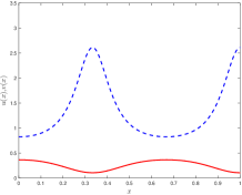
(b) $v(0)=0.3632$

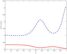
(c) $v(0)=0.3284$

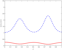
(d) $v(0)=0.2721$

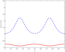
(e) $v(0)=0.2565$

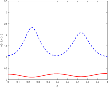
(f) $v(0)=0.2397$

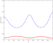
(g) $v(0)=0.1357$

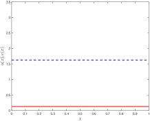
(h) $v(0)=0.1250$

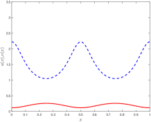
(i) $v(0)=0.11523$

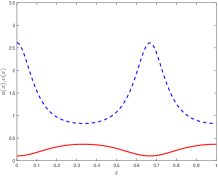
(j) $v(0)=0.1040$

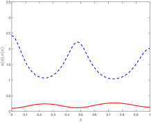
(k) $v(0)=0.0984$

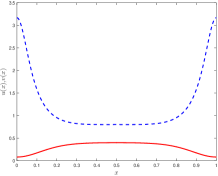
(l) $v(0)=0.0793$

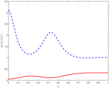
(m) $v(0)=0.0569$

Figure 4: The $13$ solutions announced in Theorem 1.1 for $d=0.005$. They can be replaced on the bifurcation diagram using the value of $v(0)$. $u$ is represented in dashed blue, and $v$ in red. We give additional information about the proof for each of these solutions in Table 1, and discuss their stability in Section 7.

Label for the solution (see Figure 4)	$m$ used for the proof	$\nu$ used for the proof	Validation radius
(a)	500	1.06	$2.5968\times 10^{-11}$
(b)	500	1.06	$9.8961\times 10^{-12}$
(c)	500	1.06	$7.2076\times 10^{-11}$
(d)	500	1.06	$7.8228\times 10^{-11}$
(e)	500	1.06	$5.7165\times 10^{-12}$
(f)	500	1.06	$1.0104\times 10^{-10}$
(g)	700	1.055	$7.7146\times 10^{-11}$
(h)	500	1.06	$2.9001\times 10^{-12}$
(i)	500	1.06	$5.0578\times 10^{-12}$
(j)	500	1.06	$6.4651\times 10^{-12}$
(k)	700	1.055	$8.1462\times 10^{-11}$
(l)	500	1.06	$1.6680\times 10^{-11}$
(m)	500	1.06	$4.2505\times 10^{-11}$

Table 1: For each solution displayed in Figure 4, we give the dimension $m$ that was used for the finite dimensional projection, the weight $\nu$ that was chosen for the space $\mathcal{X}_{\nu}$, and a validation radius $r$ for which the proof is successful, with those parameters $m$ and $\nu$.

6 Framework for the instability of steady states

In this section, we focus on the stability of the steady states whose existence we proved in the Sections 4 to 5. More precisely, we consider the cross-diffusion system (2) in the triangular case $d_{21}=0$ and with space dimension one ($\Omega=(0,1)$),

$$\left\{\begin{aligned} &\frac{\partial u}{\partial t}=\frac{\partial^{2}}{\partial x^{2}}\left((d_{1}+d_{12}v)u\right)+(r_{1}-a_{1}u-b_{1}v)u,\quad&\text{on }\mathbb{R}_{+}\times(0,1),\\ &\frac{\partial v}{\partial t}=d_{2}\frac{\partial^{2}v}{\partial x^{2}}+(r_{2}-b_{2}u-a_{2}v)v,\quad&\text{on }\mathbb{R}_{+}\times(0,1),\\ &\frac{\partial u}{\partial x}(t,0)=0=\frac{\partial u}{\partial x}(t,1),\quad&\text{on }\mathbb{R}_{+},\\ &\frac{\partial v}{\partial x}(t,0)=0=\frac{\partial v}{\partial x}(t,1),\quad&\text{on }\mathbb{R}_{+}.\end{aligned}\right.$$ (31)

Let $(u,v)=(u(x),v(x))$ be a steady state of (31). The linearization of (31), around the steady state $(u,v)$ yields the eigenvalue problem

$$\left\{\begin{aligned} &d_{1}\xi^{\prime\prime}+d_{12}\left(v^{\prime\prime}\xi+2v^{\prime}\xi^{\prime}+v\xi^{\prime\prime}+\eta^{\prime\prime}u+2\eta^{\prime}u^{\prime}+\eta u^{\prime\prime}\right)+r_{1}\xi-2a_{1}u\xi-b_{1}(v\xi+\eta u)=\lambda\xi,\quad&\text{on }(0,1),\\ &d_{2}\eta^{\prime\prime}+r_{2}\eta-b_{2}(u\eta+\xi v)-2a_{2}v\eta=\lambda\eta,\quad&\text{on }(0,1),\\ &\xi^{\prime}(0)=\xi^{\prime}(1)=0,\\ &\eta^{\prime}(0)=\eta^{\prime}(1)=0,\end{aligned}\right.$$ (32)

where the functions $(\xi,\eta)=(\xi(x),\eta(x))$ form the eigenfunction and $\lambda$ is the eigenvalue. As announced in the introduction, we aim at proving that most of the steady states obtained in Section 5 are unstable, by showing that the eigenproblem (32) admits an unstable eigenvalue, i.e. there exists a solution $\left((\xi,\eta),\lambda\right)$ of (32) such that $\Re(\lambda)>0$. The approach is similar to the one used in Section 4: we first reformulate (32) into an equivalent problem more amenable to validated numerics, and then use Theorem 2.1 to prove the existence of an unstable eigenvalue. For this, we again follow the algorithm outlined at the end of Section 2.

6.1 Proof of instability: the function $\bm{F}$

As we did for the steady states, we look for the eigenfunctions $(\xi,\eta)$ as cosine series. We point out that the steady state $(u,v)$ in (32) are non constant functions which have been obtained in Sections 4 and 5. If we directly expand (32) on the Fourier basis, the dominant terms would not be diagonal. We take care of this issue by transforming (32) into an equivalent generalized eigenvalue problem which has an autonomous second order terms.

The two equations in (32) can be rewritten as

$$M_{1}\begin{pmatrix}\xi^{\prime\prime}\\ \eta^{\prime\prime}\end{pmatrix}+M_{2}\begin{pmatrix}\xi^{\prime}\\ \eta^{\prime}\end{pmatrix}+M_{3}\begin{pmatrix}\xi\\ \eta\end{pmatrix}=\lambda\begin{pmatrix}\xi\\ \eta\end{pmatrix},$$ (33)

where

$$M_{1}=\begin{pmatrix}d_{1}+d_{12}v&d_{12}u\\ 0&d_{2}\end{pmatrix},\ M_{2}=\begin{pmatrix}2d_{12}v^{\prime}&2d_{12}u^{\prime}\\ 0&0\end{pmatrix},\ M_{3}=\begin{pmatrix}d_{12}v^{\prime\prime}+r_{1}-2a_{1}u-b_{1}v&d_{12}u^{\prime\prime}-b_{1}u\\ -b_{2}v&r_{2}-b_{2}u-2a_{2}v\end{pmatrix}.$$

Introducing $p=\frac{1}{d_{1}+d_{12}v}$ as in Section 4, and knowing that $p(x)>0$ for any $x\in[0,1]$, we can express the inverse of $M_{1}$ as:

$$M_{1}^{-1}=\begin{pmatrix}\frac{1}{d_{1}+d_{12}v}&-\frac{d_{12}u}{d_{2}(d_{1}+d_{12}v)}\\ 0&\frac{1}{d_{2}}\end{pmatrix}=\begin{pmatrix}p&-\frac{d_{12}up}{d_{2}}\\ 0&\frac{1}{d_{2}}\end{pmatrix}.$$

We multiply (33) by $M_{1}^{-1}$ and obtain the following equivalent formulation for (32):

$$\left\{\begin{aligned} &\xi^{\prime\prime}+c_{1}\xi^{\prime}+c_{2}\eta^{\prime}+c_{3}\xi+c_{4}\eta+c_{5}\lambda\xi+c_{6}\lambda\eta=0,\quad&\text{on }(0,1),\\ &\eta^{\prime\prime}+c_{7}\xi+c_{8}\eta+c_{9}\lambda\eta=0,\quad&\text{on }(0,1),\\ &\xi^{\prime}(0)=\xi^{\prime}(1)=0,\\ &\eta^{\prime}(0)=\eta^{\prime}(1)=0,\end{aligned}\right.$$ (34)

where the functions $\left(c_{j}\right)_{1\leq j\leq 9}$ depend on the steady state $(u,v)$ (and on the parameters of the cross-diffusion system), and are given by

$$c_{1}=2d_{12}pv^{\prime},\quad c_{2}=2d_{12}pu^{\prime},\quad c_{3}=(r_{1}-2a_{1}u-b_{1}v+d_{12}v^{\prime\prime})p+\frac{d_{12}b_{2}}{d_{2}}uvp,$$

$$c_{4}=(d_{12}u^{\prime\prime}-b_{1}u)p-\frac{d_{12}}{d}up(r_{2}-b_{2}u-2a_{2}v),\quad c_{5}=-p,\quad c_{6}=\frac{d_{12}}{d_{2}}up,$$

$$c_{7}=-\frac{b_{2}}{d_{2}}v,\quad c_{8}=\frac{1}{d_{2}}(r_{2}-b_{2}u-2a_{2}v),\quad c_{9}=-\frac{1}{d_{2}}.$$ (35)

6.1.1 The algebraic system in Fourier space and the $\bm{F=0}$ formulation

Expanding the eigenfunctions in cosine series

$$\xi(x)=\xi_{0}+2\sum_{k\geq 1}\xi_{k}\cos(k\pi x),\quad\eta(x)=\eta_{0}+2\sum_{k\geq 1}\eta_{k}\cos(k\pi x),$$

and inserting these expansions in (34), we end up with

$$\left\{\begin{aligned} &-(\pi k)^{2}\xi_{k}-(c_{1}\bullet K\xi)_{k}-(c_{2}\bullet K\eta)_{k}+(c_{3}\ast\xi)_{k}+(c_{4}\ast\eta)_{k}+\lambda(c_{5}\ast\xi)_{k}+\lambda(c_{6}\ast\eta)_{k}=0,\quad&\forall~{}k\in\mathbb{N},\\ &-(\pi k)^{2}\eta_{k}+(c_{7}\ast\xi)_{k}+(c_{8}\ast\eta)_{k}+\lambda(c_{9}\ast\eta)_{k}=0,\quad&\forall~{}k\in\mathbb{N}.\end{aligned}\right.$$ (36)

Again, we identify the functions $\xi$, $\eta$ and $c_{j}$ with their sequence of Fourier coefficients.

Remark 6.1.

Reset of some notations. To maintain the same notations as in Theorem 2.1, we are going to redefine the appropriate $\mathcal{X}$, $X$, $F$, $\bar{X}$, $A$ and $A^{{\dagger}}$ corresponding to the eigenproblem (34). Henceforth, we forget about the definition of this symbols that was given in Section 4, and give new ones in the sequel.

For $\gamma>1$, we define $\mathcal{X}_{\gamma}=\left(\ell^{1}_{\gamma}\right)^{2}\times\mathbb{C}$ and denote by $X=(\xi,\eta,\lambda)$ any element in $\mathcal{X}_{\gamma}$. We point out that in Section 4 we could restrict ourselves to real sequences because we were only looking for real solutions, but this is no longer the case here since we may encounter complex conjugate eigenvalues and eigenvectors. We endow $\mathcal{X}_{\gamma}$ with the norm

$$\left\|X\right\|_{\mathcal{X}_{\gamma}}=\left\|\xi\right\|_{\gamma}+\left\|\eta\right\|_{\gamma}+\left|\lambda\right|,$$

which makes it a Banach space. We then fix an index $k_{0}\in\mathbb{N}$ and define the function $F=(F^{(\xi)},F^{(\eta)},F^{(\lambda)})$ acting on $\mathcal{X}_{\gamma}$ by

$$F_{k}^{(\xi)}(X)=-(\pi k)^{2}\xi_{k}-(c_{1}\bullet K\xi)_{k}-(c_{2}\bullet K\eta)_{k}+(c_{3}\ast\xi)_{k}+(c_{4}\ast\eta)_{k}+\lambda(c_{5}\ast\xi)_{k}+\lambda(c_{6}\ast\eta)_{k}, \forall~{}k\in\mathbb{N},$$

$$F_{k}^{(\eta)}(X)=-(\pi k)^{2}\eta_{k}+(c_{7}\ast\xi)_{k}+(c_{8}\ast\eta)_{k}+\lambda(c_{9}\ast\eta)_{k}, \forall~{}k\in\mathbb{N},$$

$$F^{(\lambda)}(X)=\xi_{k_{0}}-1.$$

Notice that the only difference between $F(X)=0$ and system (36) is the equation $\xi_{k_{0}}=1$. The role of this additional constraint is to normalise the eigenfunction and hence to isolate the potential solutions of $F$. Indeed, we can not hope to successfully use Theorem 2.1, which is based on a contraction argument, if the zeros of $F$ are not isolated. We point out that many different conditions could have been added to isolate the solution, and that this specific choice is rather arbitrary.

We now state the precise link between $F$ and our stability problem.

Lemma 6.2.

Assume that $(u,v)$ is a positive stationary solution of (31) and that there exists $\gamma>1$ such that the Fourier coefficients of the functions $\left(c_{j}\right)_{1\leq j\leq 9}$, defined in (35), belong to $\ell^{1}_{\gamma}(\mathbb{R})$. Fix $k_{0}\in\mathbb{N}$ and suppose that there exists $X=(\xi,\eta,\lambda)\in\mathcal{X}_{\gamma}$, with $\Re(\lambda)>0$, such that $F(X)=0$. Then the steady state $(u,v)$ is linearly unstable.

Proof.

As for Lemma 4.1, the proof just consists in checking that the regularity (i.e. the fact that the Fourier coefficients belongs to $\ell^{1}_{\gamma}$) of the solution $X$ and of the data $\left(c_{j}\right)_{1\leq j\leq 9}$ allows to rigorously backtrack the manipulations made to obtain $F$ from the eigenproblem (32). ∎

We point out that the assumption that $u$ and $v$ are positive, is in fact only needed here to ensure that $p$ is well defined. Concerning the assumption on the functions $\left(c_{j}\right)_{1\leq j\leq 9}$, the method developed in Sections 4 to 5 naturally provides us with steady states $(u,v)$ for which the Fourier coefficients of $u$, $v$ (and $p$) belong to $\ell^{1}_{\nu}$, for some $\nu>1$. However, since some of the $c_{j}$ involve derivatives of $u$ and $v$, we can only get that their Fourier coefficients belong to $\ell^{1}_{\gamma}$ for $\gamma<\nu$. We give more details and explicit estimates right below.

6.1.2 About the functions $\bm{c_{j}}$

The function $F$ depends on the Fourier coefficients of $\left(c_{j}\right)_{1\leq j\leq 9}$, which themselves depend on the steady state $(u,v)$. The method described in Sections 4 to 5 (in particular Proposition 4.5) provides us with an approximate steady state, in the form of Fourier sequences $(\bar{v},\bar{w},\bar{p},\bar{s})$, together with a validation radius $r_{\nu}$ which gives an upper bound of the distance (in the $\ell^{1}_{\nu}$ norm) between the approximate steady state and the genuine one.

Remark 6.3.

From now on, we denote $r_{\nu}$ the validation radius obtained in the computation of the steady states. This validation radius was simply denoted by $r$ in Section 4 and 5, but this new notation should avoid possible confusions with the validation radius that we are going to consider for the eigenvalue problem.

More precisely, the steady state (in the $(v,w,p,s)$ coordinates) is proved to exist in the form

$$v=\bar{v}+\varepsilon_{v},\quad w=\bar{w}+\varepsilon_{w},\quad p=\bar{p}+\varepsilon_{p},\quad s=\bar{s}+\varepsilon_{s},$$

where the $(\bar{v},\bar{w},\bar{p},\bar{s})$ are finite Fourier sequences that we have explicitly on our computer, and $\left\|\varepsilon_{v}\right\|_{\nu}+\left\|\varepsilon_{w}\right\|_{\nu}+\left\|\varepsilon_{p}\right\|_{\nu}+\left\|\varepsilon_{s}\right\|_{\nu}\leq r_{\nu}$, where $r_{\nu}$ is the radius provided by the proof.

Therefore, we can also represent each $c_{j}$ as

$$c_{j}=\bar{c}_{j}+\varepsilon_{j},$$

where $\bar{c}_{j}$ is a finite sequence of Fourier coefficients and $\left\|\varepsilon_{j}\right\|_{\gamma}\leq\epsilon_{j}(\gamma)$. In this section, we provide formulas for the finite sequences $\bar{c}_{j}$ and the upper bounds $\epsilon_{j}(\gamma)$ on the distance (in $\ell^{1}_{\gamma}$) between $\bar{c}_{j}$ and $c_{j}$ .

The first step is to provide an enclosure for $u$ in the form $u=\bar{u}+\varepsilon_{u}$. Remembering that $u(x)=p(x)w(x)$, and hence $u=p*w$, we have

$$u=\bar{p}\ast\bar{w}+\bar{p}\ast\varepsilon_{w}+\varepsilon_{p}\ast\bar{w}+\varepsilon_{p}\ast\varepsilon_{w}.$$

Therefore, we can define $\bar{u}=\bar{p}\ast\bar{w}$, and $\varepsilon_{u}=\bar{p}\ast\varepsilon_{w}+\varepsilon_{p}\ast\bar{w}+\varepsilon_{p}\ast\varepsilon_{w}$. By Lemma 3.3, a bound for the norm of $\varepsilon_{u}$ is given as $\left\|\varepsilon_{u}\right\|_{\nu}\leq(\left\|\bar{p}\right\|_{\nu}+\left\|\bar{w}\right\|_{\nu})r_{\nu}+\frac{r_{\nu}^{2}}{4}$, where we used that $\left\|\varepsilon_{p}\right\|_{\nu}\left\|\varepsilon_{w}\right\|_{\nu}\leq\frac{1}{4}(\left\|\varepsilon_{p}\right\|_{\nu}+\left\|\varepsilon_{w}\right\|_{\nu})^{2}$. For further use, we define $\epsilon_{u}=(\left\|\bar{p}\right\|_{\nu}+\left\|\bar{w}\right\|_{\nu})r_{\nu}+\frac{r_{\nu}^{2}}{4}$.

The second step is to derive estimates on derivatives.

Definition 6.4.

Denote by $K$ the (unbounded) linear operator such that, for all $z$ in $\ell^{1}_{\nu}$

$$\left(Kz\right)_{k}=\pi kz_{k},\quad\forall k\geq 0.$$

Up to a change of sign (depending on whether we consider the cosine or sine expansion), $Kz$ is nothing but the sequence of Fourier coefficients of the derivative of the function $z(x)$.

Lemma 6.5.

Let $1<\gamma<\nu$ and $z\in\ell^{1}_{\nu}$. Then

$$\left\|Kz\right\|_{\gamma}\leq\Upsilon_{\gamma,\nu}^{1}\left\|z\right\|_{\nu},\quad\left\|K^{2}z\right\|_{\gamma}\leq\Upsilon_{\gamma,\nu}^{2}\left\|z\right\|_{\nu},$$

where

$$\Upsilon_{\gamma,\nu}^{1}=\left\{\begin{aligned} &\frac{\gamma}{\nu},\quad&\text{if }\gamma<e^{-1}\nu\\ &\frac{e^{-1}}{\ln\frac{\nu}{\gamma}},\quad&\text{otherwise,}\end{aligned}\right.\qquad\qquad\text{and}\qquad\qquad\Upsilon_{\gamma,\nu}^{2}=\left\{\begin{aligned} &\frac{\gamma}{\nu},\quad&\text{if }\gamma<e^{-2}\nu\\ &\left(\frac{2e^{-1}}{\ln\frac{\nu}{\gamma}}\right)^{2},\quad&\text{otherwise.}\end{aligned}\right.$$

Proof.

We estimate

$$\left\|Kz\right\|_{\gamma} =2\sum_{k\geq 1}k\left|z_{k}\right|\gamma^{k}$$

$$=2\sum_{k\geq 1}k\left(\frac{\gamma}{\nu}\right)^{k}\left|z_{k}\right|\nu^{k}$$

$$\leq\left\|z\right\|_{\nu}\sup\limits_{k\geq 1}k\left(\frac{\gamma}{\nu}\right)^{k}.$$

The constant $\Upsilon_{\gamma,\nu}^{1}$ is the maximum (on $[1,+\infty)$) of the function $k\mapsto k\left(\frac{\gamma}{\nu}\right)^{k}$. Similarly, $\Upsilon_{\gamma,\nu}^{2}$ is the maximum (on $[1,+\infty)$) of the function $k\mapsto k^{2}\left(\frac{\gamma}{\nu}\right)^{k}$. ∎

For $v=\bar{v}+\varepsilon_{v}$ we have $Kv=K\bar{v}+K\varepsilon_{v}$. The sequence $K\bar{v}$ can be rigorously computed, being finite dimensional, while by the Lemma 6.5 $\left\|K\varepsilon_{v}\right\|_{\gamma}\leq\Upsilon_{\gamma,\nu}^{1}r_{\nu}$. The same argument used to derive $\bar{u}$ and $\epsilon_{u}$ and the application of the Lemma 6.5 when requested, provide the following expressions for $\bar{c}_{j}$, and $\epsilon_{j}(\gamma)$:

$$\bar{c}_{1}=-2d_{12}(K\bar{v}\star\bar{p}),\quad\bar{c}_{2}=-2d_{12}(K\bar{u}\star\bar{p}),\quad\bar{c}_{3}=((r_{1}-2a_{1}\bar{u}-b_{1}\bar{v}+d_{12}K\bar{s})\ast\bar{p})+\frac{d_{12}b_{2}}{d_{2}}(\bar{u}\ast\bar{v}\ast\bar{p}),$$

$$\bar{c}_{4}=((-d_{12}K^{2}\bar{u}-b_{1}\bar{u})\ast\bar{p})-\frac{d_{12}}{d}(\bar{u}\ast\bar{p}\ast(r_{2}-b_{2}\bar{u}-2a_{2}\bar{v})),\quad\bar{c}_{5}=-\bar{p},\quad\bar{c}_{6}=\frac{d_{12}}{d_{2}}(\bar{u}\ast\bar{p}),$$

$$\bar{c}_{7}=-\frac{b_{2}}{d_{2}}\bar{v},\quad\bar{c}_{8}=\frac{1}{d_{2}}(r_{2}-b_{2}\bar{u}-2a_{2}\bar{v}),\quad\bar{c}_{9}=-\frac{1}{d_{2}},$$

together with

$$\epsilon_{1}(\gamma)=2d_{12}(\left\|K\bar{v}\right\|_{\gamma}r_{\nu}+\left\|\bar{p}\right\|_{\gamma}\Upsilon_{\gamma,\nu}^{1}r_{\nu}+\Upsilon_{\gamma,\nu}^{1}r_{\nu}^{2}),\quad\epsilon_{2}(\gamma)=2d_{12}(\left\|K\bar{u}\right\|_{\gamma}r_{\nu}+\left\|\bar{p}\right\|_{\gamma}\Upsilon_{\gamma,\nu}^{1}\epsilon_{u}+\Upsilon_{\gamma,\nu}^{1}\epsilon_{u}r_{\nu}),$$

$$\epsilon_{3}(\gamma) =\left\|r_{1}-2a_{1}\bar{u}-b_{1}\bar{v}+d_{12}K\bar{s}\right\|_{\gamma}r_{\nu}+(2a_{1}\epsilon_{u}+b_{1}r_{\nu}+d_{12}\Upsilon_{\gamma,\nu}^{1}r_{\nu})\left\|\bar{p}\right\|_{\gamma}+(2a_{1}\epsilon_{u}+b_{1}r_{\nu}+d_{12}\Upsilon_{\gamma,\nu}^{1}r_{\nu})r_{\nu}$$

$$\quad+\frac{d_{12}b_{2}}{d_{2}}(\left\|\bar{u}\ast\bar{v}\right\|_{\gamma}r_{\nu}+\left\|\bar{u}\ast\bar{p}\right\|_{\gamma}r_{\nu}+\left\|\bar{v}\ast\bar{p}\right\|_{\gamma}\epsilon_{u}+\left\|\bar{u}\right\|_{\gamma}r_{\nu}^{2}+\left\|\bar{v}\right\|_{\gamma}\epsilon_{u}r_{\nu}+\left\|\bar{p}\right\|_{\gamma}\epsilon_{u}r_{\nu}+\epsilon_{u}r_{\nu}^{2}),$$

$$\epsilon_{4}(\gamma) =\left\|-d_{12}K^{2}\bar{u}-b_{1}\bar{u}\right\|_{\gamma}r_{\nu}+(d_{12}\Upsilon_{\gamma,\nu}^{2}\epsilon_{u}+b_{1}\epsilon_{u})\left\|\bar{p}\right\|_{\gamma}+(d_{12}\Upsilon_{\gamma,\nu}^{2}\epsilon_{u}+b_{1}\epsilon_{u})r_{\nu}$$

$$\quad+\frac{d_{12}}{d_{2}}\left(\left\|\bar{u}\ast\bar{p}\right\|_{\gamma}(b_{2}\epsilon_{u}+2a_{2}r_{\nu})+\left\|\bar{u}\ast(r_{2}-b_{2}\bar{u}-2a_{2}\bar{v})\right\|_{\gamma}r_{\nu}\right.$$

$$\qquad\qquad\left.+\left\|\bar{p}\ast(r_{2}-b_{2}\bar{u}-2a_{2}\bar{v})\right\|_{\gamma}\epsilon_{u}+\epsilon_{u}r_{\nu}(b_{2}\epsilon_{u}+2a_{2}r_{\nu})\right),$$

$$\epsilon_{5}=r_{\nu},\quad\epsilon_{6}(\gamma)=\frac{d_{12}}{d_{2}}(\left\|\bar{u}\right\|_{\gamma}r_{\nu}+\left\|\bar{u}\ast\bar{p}\right\|_{\gamma}\epsilon_{u}+\epsilon_{u}r_{\nu}),\quad\epsilon_{7}=\frac{b_{2}}{d_{2}}r_{\nu},\quad\epsilon_{8}=\frac{1}{d_{2}}(b_{2}\epsilon_{u}+2a_{2}r_{\nu}),\quad\epsilon_{9}=0.$$

6.2 Proof of instability: the operators $\bm{A}$ and $\bm{A^{\dagger}}$

We now introduce the approximate solution and linear operators needed to apply Theorem 2.1 in the context of the eigenproblem (32).

Compared to the situation of Section 4.2, we have here an additional difficulty due to the fact that the function $F$ depends on the coefficients $\left(c_{j}\right)_{1\leq j\leq 9}$, which (as detailed above) are only known up to an error bound. This motivates the splitting of the function $F$ into two parts, one containing the known terms $\bar{c}_{j}$ and the other one containing the remainder terms $\varepsilon_{j}$. More precisely, we define $\bar{F}$ by

$$\bar{F}_{k}^{(\xi)}(X)=-(\pi k)^{2}\xi_{k}-(\bar{c}_{1}\bullet K\xi)_{k}-(\bar{c}_{2}\bullet K\eta)_{k}+(\bar{c}_{3}\ast\xi)_{k}+(\bar{c}_{4}\ast\eta)_{k}+\lambda(\bar{c}_{5}\ast\xi)_{k}+\lambda(\bar{c}_{6}\ast\eta)_{k}, \forall~{}k\in\mathbb{N},$$

$$\bar{F}_{k}^{(\eta)}(X)=-(\pi k)^{2}\eta_{k}+(\bar{c}_{7}\ast\xi)_{k}+(\bar{c}_{8}\ast\eta)_{k}+\lambda(\bar{c}_{9}\ast\eta)_{k}, \forall~{}k\in\mathbb{N},$$

$$\bar{F}^{(\lambda)}(X)=\xi_{k_{0}}-1,$$ (37)

and $\mathcal{E}_{F}$ as

$$\left(\mathcal{E}_{F}\right)_{k}^{(\xi)}(X)=-(\varepsilon_{1}\bullet K\xi)_{k}-(\varepsilon_{2}\bullet K\eta)_{k}+(\varepsilon_{3}\ast\xi)_{k}+(\varepsilon_{4}\ast\eta)_{k}+\lambda(\varepsilon_{5}\ast\xi)_{k}+\lambda(\varepsilon_{6}\ast\eta)_{k}, \forall~{}k\in\mathbb{N},$$

$$\left(\mathcal{E}_{F}\right)_{k}^{(\eta)}(X)=(\varepsilon_{7}\ast\xi)_{k}+(\varepsilon_{8}\ast\eta)_{k}+\lambda(\varepsilon_{9}\ast\eta)_{k}, \forall~{}k\in\mathbb{N},$$

$$\left(\mathcal{E}_{F}\right)^{(\lambda)}(X)=0,$$ (38)

so that $F=\bar{F}+\mathcal{E}_{F}$.

Then, extending again the notations introduced in Definition 3.5, we denote

$$\hat{X}^{n}=(\hat{\xi}^{n},\hat{\eta}^{n},\lambda).$$

Notice that the truncation parameter $n$ does not need to be (and in practice is not) the same as the truncation parameter $m$ used for the steady states. However, we require $n>k_{0}$, so that the isolating condition that we imposed is incorporated in the finite dimensional projection. We also define

$$\hat{F}^{n}=\left(\left(\bar{F}^{(\xi)}_{k}\right)_{0\leq k<n},\left(\bar{F}^{(\eta)}_{k}\right)_{0\leq k<n},\bar{F}^{(\lambda)}\right).$$

We consider $\hat{F}^{n}$ as acting on truncated sequences $\hat{X}^{n}$ only, so that we can see it as a function mapping $\mathbb{C}^{2n+1}$ to itself. Therefore, finding $\hat{X}^{n}$ such that $\hat{F}^{n}(\hat{X}^{n})=0$ is a finite dimensional problem that can be solved numerically. Notice that crucially, $\hat{F}$ is a finite dimensional projection of $\bar{F}$ rather than of $F$, so it only depends on coefficients that are known explicitly.

We now assume that we have computed numerically a zero of $\hat{F}^{n}$, and denote it $\bar{X}$. The next step is to define $A^{{\dagger}}$ and $A$. Again, we are going to take for $A^{{\dagger}}$ an approximation of $DF(\bar{X})$, with a diagonal tail. More precisely, we define $A^{{\dagger}}$ (acting on $X=(\xi,\eta,\lambda)\in\mathcal{X}_{\gamma}$), as

$$\widehat{A^{{\dagger}}X}^{n}=D\hat{F}^{n}(\bar{X})\hat{X}^{n},$$

and

$$\left(A^{{\dagger}}X\right)_{k}=\left(-(\pi k)^{2}\xi_{k},-(\pi k)^{2}\eta_{k}\right),\quad\forall~{}k\geq n.$$

Then, we consider $\hat{A}^{n}$ a numerically computed inverse of $D\hat{F}^{n}(\bar{X})$ and define $A$ (acting on $X=(\xi,\eta,\lambda)\in\mathcal{X}_{\gamma}$), as

$$\widehat{AX}^{n}=\hat{A}^{n}\hat{X}^{n},$$

and

$$\left(AX\right)_{k}=\left(-(\pi k)^{-2}\xi_{k},-(\pi k)^{-2}\eta_{k}\right),\quad\forall~{}k\geq n.$$

Remark 6.6.

As in Remark (4.2), we point out the diagonal dominant behaviour of the derivative $DF(\bar{X})$ is the result of some preliminary manipulations done on the differential system, in this case the multiplication of the eigenproblem (32) by $M_{1}^{-1}$.

The definition of the tail part of $A$ and the fact that $\ell^{1}_{\gamma}$ is an algebra for both convolution products $\ast$ and $\bullet$ (see Lemma 3.3) ensure that $AF$ does map $\mathcal{X}_{\gamma}$ into itself as requested to apply Theorem 2.1.

Adopting a similar bloc notation as introduced in Section 4.3.2, we write

$$A=\begin{pmatrix}A^{(\xi,\xi)}&A^{(\xi,\eta)}&A^{(\xi,\lambda)}\\ A^{(\eta,\xi)}&A^{(\eta,\eta)}&A^{(\eta,\lambda)}\\ A^{(\lambda,\xi)}&A^{(\lambda,\eta)}&A^{(\lambda,\lambda)}\end{pmatrix},$$

and define

$$\Theta_{A}^{(\xi)}=\VERT A^{(\xi,\xi)}\VERT_{\gamma}+\VERT A^{(\eta,\xi)}\VERT_{\gamma}+\VERT A^{(\lambda,\xi)}\VERT_{\gamma},\quad\Theta_{A}^{(\eta)}=\VERT A^{(\xi,\eta)}\VERT_{\gamma}+\VERT A^{(\eta,\eta)}\VERT_{\gamma}+\VERT A^{(\lambda,\eta)}\VERT_{\gamma},$$

$$\Theta_{A}^{(\lambda)}=\|A^{(\xi,\lambda)}\|_{\gamma}+\|A^{(\eta,\lambda)}\|_{\gamma}+|A^{(\lambda,\lambda)}|.$$

6.3 Proof of instability: the bounds $\bm{Y}$ and $\bm{Z_{i}(r)}$

Consider $\mathcal{X}_{\gamma}$, $F$, $\bar{X}=(\bar{\xi},\bar{\eta},\bar{\lambda})$, $A$, $A^{{\dagger}}$ as defined in Sections 6.1-6.2. Now we derive computable bounds $Y$, $Z_{0}$, $Z_{1}$ and $Z_{2}$ satisfying (5)-(8) (for $\mathcal{X}=\mathcal{X}_{\gamma}$).

6.3.1 The bound $\bm{Y}$

Lemma 6.7.

Define

$$Y =\left\|A\bar{F}(\bar{X})\right\|_{\mathcal{X}_{\gamma}}+\Theta_{A}^{(\xi)}\left(\left\|K\bar{\xi}\right\|_{\gamma}\epsilon_{1}(\gamma)+\left\|K\bar{\eta}\right\|_{\gamma}\epsilon_{2}(\gamma)+\left\|\bar{\xi}\right\|_{\gamma}(\epsilon_{3}(\gamma)+|\bar{\lambda}|\epsilon_{5}(\gamma))+\left\|\bar{\eta}\right\|_{\gamma}(\epsilon_{4}(\gamma)+|\bar{\lambda}|\epsilon_{6}(\gamma))\right)$$

$$\quad+\Theta_{A}^{(\eta)}\left(\left\|\bar{\xi}\right\|_{\gamma}\epsilon_{7}(\gamma)+\left\|\bar{\eta}\right\|_{\gamma}(\epsilon_{8}(\gamma)+|\bar{\lambda}|\epsilon_{9}(\gamma))\right).$$ (39)

Then $Y\geq\left\|AF(\bar{X})\right\|_{\gamma}$.

Proof.

Using the splitting $F=\bar{F}+\mathcal{E}_{F}$ introduced in (6.2)-(6.2), we bound separately $\left\|A\bar{F}(\bar{X})\right\|_{\gamma}$ and $\left\|A\mathcal{E}_{F}(\bar{X})\right\|_{\gamma}$. $A\bar{F}(\bar{X})$ only has finitely many non zero coefficients, therefore $\left\|A\bar{F}(\bar{X})\right\|_{\gamma}$ can be evaluated on a computer (using interval arithmetic to control the round-off errors).

Concerning the second term, we have that

$$\left\|\mathcal{E}_{F}^{(\xi)}(\bar{X})\right\|_{\gamma} \leq\left\|K\bar{\xi}\right\|_{\gamma}\epsilon_{1}(\gamma)+\left\|K\bar{\eta}\right\|_{\gamma}\epsilon_{2}(\gamma)+\left\|\bar{\xi}\right\|_{\gamma}(\epsilon_{3}(\gamma)+|\bar{\lambda}|\epsilon_{5}(\gamma))+\left\|\bar{\eta}\right\|_{\gamma}(\epsilon_{4}(\gamma)+|\bar{\lambda}|\epsilon_{6}(\gamma)),$$

$$\left\|\mathcal{E}_{F}^{(\eta)}(\bar{X})\right\|_{\gamma} \leq\left\|\bar{\xi}\right\|_{\gamma}\epsilon_{7}(\gamma)+\left\|\bar{\eta}\right\|_{\gamma}(\epsilon_{8}(\gamma)+|\bar{\lambda}|\epsilon_{9}(\gamma)).$$

Thus

$$\left\|A\mathcal{E}_{F}(\bar{X})\right\|_{\mathcal{X}_{\gamma}} \leq\Theta_{A}^{(\xi)}\left(\left\|K\bar{\xi}\right\|_{\gamma}\epsilon_{1}(\gamma)+\left\|K\bar{\eta}\right\|_{\gamma}\epsilon_{2}(\gamma)+\left\|\bar{\xi}\right\|_{\gamma}(\epsilon_{3}(\gamma)+|\bar{\lambda}|\epsilon_{5}(\gamma))+\left\|\bar{\eta}\right\|_{\gamma}(\epsilon_{4}(\gamma)+|\bar{\lambda}|\epsilon_{6}(\gamma))\right)$$

$$\quad+\Theta_{A}^{(\eta)}\left(\left\|\bar{\xi}\right\|_{\gamma}\epsilon_{7}(\gamma)+\left\|\bar{\eta}\right\|_{\gamma}(\epsilon_{8}(\gamma)+|\bar{\lambda}|\epsilon_{9}(\gamma))\right).$$

The sum of the last expression and $\left\|A\bar{F}(\bar{X})\right\|_{\gamma}$ gives $Y$. ∎

6.3.2 The bound $\bm{Z_{0}}$

Arguing exactly as in Section 4.3.2, we define

$$Z_{0}=\max\left[\Theta_{I-AA^{{\dagger}}}^{(\xi)},\Theta_{I-AA^{{\dagger}}}^{(\eta)},\Theta_{I-AA^{{\dagger}}}^{(\lambda)}\right].$$ (40)

6.3.3 The bound $\bm{Z_{1}}$

Now we focus on providing a bound $Z_{1}$ satisfying (7).

Lemma 6.8.

Let $\hat{\alpha}^{n}_{\xi},\hat{\alpha}^{n}_{\eta}$ be vectors in $\mathbb{C}^{2n+1}$ each, defined as

$$\left(\hat{\alpha}^{n}_{\xi}\right)_{0}=\begin{pmatrix}\Phi_{0}^{n}(\bar{c}_{3}-K\bar{c}_{1}+\bar{\lambda}\bar{c}_{5},\gamma)\\ \Phi_{0}^{n}(\bar{c}_{7},\gamma)\\ 0\end{pmatrix},\quad\left(\hat{\alpha}^{n}_{\eta}\right)_{0}=\begin{pmatrix}\Phi_{0}^{n}(\bar{c}_{4}-K\bar{c}_{2}+\bar{\lambda}\bar{c}_{6}\gamma)\\ \Phi_{0}^{n}(\bar{c}_{8}+\bar{\lambda}\bar{c}_{9},\gamma)\\ 0\end{pmatrix},$$

and for all $1\leq k<n$

$$\left(\hat{\alpha}^{n}_{\xi}\right)_{k}=\begin{pmatrix}k\Phi_{k}^{n}(\bar{c}_{1},\gamma)+\Phi_{k}^{n}(\bar{c}_{3}-K\bar{c}_{1}+\bar{\lambda}\bar{c}_{5},\gamma)\\ \Phi_{k}^{n}(\bar{c}_{7},\gamma)\end{pmatrix},\quad\left(\hat{\alpha}^{n}_{\eta}\right)_{k}=\begin{pmatrix}k\Phi_{k}^{n}(\bar{c}_{2},\gamma)+\Phi_{k}^{n}(\bar{c}_{4}-K\bar{c}_{2}+\bar{\lambda}\bar{c}_{6}\gamma)\\ \Phi_{k}^{n}(\bar{c}_{8}+\bar{\lambda}\bar{c}_{9},\gamma)\end{pmatrix}.$$

Let the operator $\tilde{K}$ acting on $\mathcal{X}_{\gamma}$ defined as

$$\tilde{K}=\begin{pmatrix}K&0&0\\ 0&0&0\\ 0&0&0\end{pmatrix},$$

where $K$ is the same operator as in Definition 6.4.

Choose $\tilde{\gamma}\in(\gamma,\nu)$ and define

$$Z_{1} =\max\left[\left\||A|\hat{\alpha}^{n}_{\xi}\right\|_{\mathcal{X}_{\gamma}},\left\||A|\hat{\alpha}^{n}_{\eta}\right\|_{\mathcal{X}_{\gamma}}\right]$$

$$\quad+\max\left[\frac{\left\|\bar{c}_{1}\right\|_{\gamma}}{\pi n}+\frac{\left\|\bar{c}_{3}-K\bar{c}_{1}+\bar{\lambda}\bar{c}_{5}\right\|_{\gamma}+\left\|\bar{c}_{7}\right\|_{\gamma}}{(\pi n)^{2}},\frac{\left\|\bar{c}_{2}\right\|_{\gamma}}{\pi n}+\frac{\left\|\bar{c}_{4}-K\bar{c}_{2}+\bar{\lambda}\bar{c}_{6}\right\|_{\gamma}+\left\|\bar{c}_{8}+\bar{\lambda}\bar{c}_{9}\right\|_{\gamma}}{(\pi n)^{2}},\right.$$

$$\qquad\qquad\left.\frac{\left\|\bar{c}_{5}\ast\bar{\xi}\right\|_{\gamma}+\left\|\bar{c}_{6}\ast\bar{\eta}\right\|_{\gamma}+\left\|\bar{c}_{9}\ast\bar{\eta}\right\|_{\gamma}}{(\pi n)^{2}}\right]$$

$$\quad+\max\left[\Theta_{A}^{(\xi)}\left(\Upsilon_{\gamma,\tilde{\gamma}}^{1}\epsilon_{1}(\tilde{\gamma})+\epsilon_{3}(\gamma)+|\bar{\lambda}|\epsilon_{5}(\gamma)\right)+\Theta_{A}^{(\eta)}\epsilon_{7}(\gamma),\right.$$

$$\qquad\qquad\left.\Theta_{A}^{(\xi)}\left(\Upsilon_{\gamma,\tilde{\gamma}}^{1}\epsilon_{2}(\tilde{\gamma})+\epsilon_{4}(\gamma)+|\bar{\lambda}|\epsilon_{6}(\gamma)\right)+\Theta_{A}^{(\eta)}\left(\epsilon_{8}(\gamma)+|\bar{\lambda}|\epsilon_{9}(\gamma)\right),\right.$$

$$\qquad\qquad\left.\Theta_{A}^{(\xi)}\left(\left\|\bar{\xi}\right\|_{\gamma}\epsilon_{5}(\gamma)+\left\|\bar{\eta}\right\|_{\gamma}\epsilon_{6}(\gamma)\right)+\Theta_{A}^{(\eta)}\left\|\bar{\eta}\right\|_{\gamma}\epsilon_{9}(\gamma)\right]$$

$$\quad+\Theta_{A\tilde{K}}^{(\xi)}\max\left[\epsilon_{1}(\gamma),\epsilon_{2}(\gamma)\right].$$ (41)

then

$$Z_{1}\geq\left\VERT A\left(DF(\bar{X})-A^{{\dagger}}\right)\right\VERT_{\mathcal{X}_{\gamma}}$$

Proof.

Using the splitting of $F$ introduced in in (6.2)-(6.2) we have

$$\left\VERT A\left(DF(\bar{X})-A^{{\dagger}}\right)\right\VERT_{\mathcal{X}_{\gamma}}\leq\left\VERT A\left(D\bar{F}(\bar{X})-A^{{\dagger}}\right)\right\VERT_{\mathcal{X}_{\gamma}}+\left\VERT AD\mathcal{E}_{F}(\bar{X})\right\VERT_{\mathcal{X}_{\gamma}}.$$

The procedure to obtain a bound for the first part on the r.h.s is similar to the one followed in Section 7 (since the remainder terms $\left(\varepsilon_{j}\right)_{1\leq j\leq 9}$ are not involved), therefore we skip most of the details. Let $X\in\mathcal{B}_{\mathcal{X}_{\gamma}}(0,1)$ and introduce $U=\left(D\bar{F}(\bar{X})-A^{{\dagger}}\right)X$. We have

$$\left\|A\left(D\bar{F}(\bar{X})-A^{{\dagger}}\right)X\right\|_{\mathcal{X}_{\gamma}} \leq\left\||A||U|\right\|_{\mathcal{X}_{\gamma}}$$

$$\leq\||A||\hat{U}^{n}|\|_{\mathcal{X}_{\gamma}}+\||A||\check{U}^{n}|\|_{\mathcal{X}_{\gamma}},$$

and we provide a bound for each term separately. For both of them, it is helpful to notice that

$$(\bar{c}_{1}\bullet K\xi)=-K(\bar{c}_{1}\star\xi)+(K\bar{c}_{1}\ast\xi),$$ (42)

and similarly for $(\bar{c}_{2}\bullet K\eta)$, this identity being nothing but $\bar{c}_{1}\xi^{\prime}=(\bar{c}_{1}\xi)^{\prime}-\bar{c}_{1}^{\prime}\xi$ written for the Fourier sequences. Using (42) and proceeding exactly as in Section 7, we obtain

$$\||A||\hat{U}^{n}|\|_{\mathcal{X}_{\gamma}}\leq\max\left[\left\||A|\hat{\alpha}^{n}_{\xi}\right\|_{\mathcal{X}_{\gamma}},\left\||A|\hat{\alpha}^{n}_{\eta}\right\|_{\mathcal{X}_{\gamma}}\right]\left\|X\right\|_{\mathcal{X}_{\gamma}}.$$ (43)

For the tail part, using Lemma 3.3, and the definition of the tail part of $A$, we compute

$$\left\||A||\check{U}^{n}|\right\|_{\mathcal{X}_{\gamma}} \leq\max\left[\frac{\left\|\bar{c}_{1}\right\|_{\gamma}}{\pi n}+\frac{\left\|\bar{c}_{3}-K\bar{c}_{1}+\bar{\lambda}\bar{c}_{5}\right\|_{\gamma}+\left\|\bar{c}_{7}\right\|_{\gamma}}{(\pi n)^{2}},\right.$$

$$\qquad\qquad\left.\frac{\left\|\bar{c}_{2}\right\|_{\gamma}}{\pi n}+\frac{\left\|\bar{c}_{4}-K\bar{c}_{2}+\bar{\lambda}\bar{c}_{6}\right\|_{\gamma}+\left\|\bar{c}_{8}+\bar{\lambda}\bar{c}_{9}\right\|_{\gamma}}{(\pi n)^{2}},\right.$$

$$\qquad\qquad\left.\frac{\left\|\bar{c}_{5}\ast\bar{\xi}\right\|_{\gamma}+\left\|\bar{c}_{6}\ast\bar{\eta}\right\|_{\gamma}+\left\|\bar{c}_{9}\ast\bar{\eta}\right\|_{\gamma}}{(\pi n)^{2}}\right]\left\|X\right\|_{\mathcal{X}_{\gamma}}.$$ (44)

It remains to estimate $\left\VERT AD\mathcal{E}_{F}(\bar{X})\right\VERT_{\mathcal{X}_{\gamma}}$. We want to proceed in a similar fashion as in Section 6.3.1 where we computed a bound for $\left\|A\mathcal{E}_{F}(\bar{X})\right\|_{\mathcal{X}_{\gamma}}$. However, we have to be slightly more careful, since $\left\VERT D\mathcal{E}_{F}(\bar{X})\right\VERT_{\mathcal{X}_{\gamma}}$ is not finite (because of the $\pi k$ terms coming from the first order derivatives). Therefore, using again (42), we separate the unbounded contributions and decompose $\mathcal{E}_{F}$ into $\mathcal{E}^{1}_{F}+\mathcal{E}^{2}_{F}$, where

$$\left(\mathcal{E}^{1}_{F}\right)_{k}^{(\xi)}(X)=-(K\varepsilon_{1}\ast\xi)_{k}-(K\varepsilon_{2}\ast\eta)_{k}+(\varepsilon_{3}\ast\xi)_{k}+(\varepsilon_{4}\ast\eta)_{k}+\lambda(\varepsilon_{5}\ast\xi)_{k}+\lambda(\varepsilon_{6}\ast\eta)_{k}, \forall~{}k\in\mathbb{N},$$

$$\left(\mathcal{E}^{1}_{F}\right)_{k}^{(\eta)}(X)=(\varepsilon_{7}\ast\xi)_{k}+(\varepsilon_{8}\ast\eta)_{k}+\lambda(\varepsilon_{9}\ast\eta)_{k}, \forall~{}k\in\mathbb{N},$$

$$\left(\mathcal{E}^{2}_{F}\right)^{(\lambda)}(X)=0,$$

and

$$\left(\mathcal{E}^{2}_{F}\right)_{k}^{(\xi)}(X)=\pi k(\varepsilon_{1}\star\xi)_{k}+\pi k(\varepsilon_{2}\star\eta)_{k}, \forall~{}k\in\mathbb{N},$$

$$\left(\mathcal{E}^{2}_{F}\right)_{k}^{(\eta)}(X)=0, \forall~{}k\in\mathbb{N},$$

$$\left(\mathcal{E}^{1}_{F}\right)^{(\lambda)}(X)=0.$$

and we provide bounds on $\left\|AD\mathcal{E}^{1}_{F}(\bar{X})X\right\|_{\mathcal{X}_{\gamma}}$ and $\left\|AD\mathcal{E}^{2}_{F}(\bar{X})X\right\|_{\mathcal{X}_{\gamma}}$, for $X=(\xi,\eta,\lambda)\in\mathcal{B}_{\mathcal{X}_{\gamma}}(0,1)$. The smoothing effect of $A$ will make the second bound finite.

First, consider

$$\left\|D\left(\mathcal{E}^{1}_{F}\right)^{(\xi)}(\bar{X})X\right\|_{\mathcal{X}_{\gamma}} \leq\left(\left\|K\varepsilon_{1}\right\|_{\gamma}+\epsilon_{3}(\gamma)+|\bar{\lambda}|\epsilon_{5}(\gamma)\right)\left\|\xi\right\|_{\gamma}+\left(\left\|K\varepsilon_{2}\right\|_{\gamma}+\epsilon_{4}(\gamma)+|\bar{\lambda}|\epsilon_{6}(\gamma)\right)\left\|\eta\right\|_{\gamma}$$

$$\quad+\left(\left\|\bar{\xi}\right\|_{\gamma}\epsilon_{5}(\gamma)+\left\|\bar{\eta}\right\|_{\gamma}\epsilon_{6}(\gamma)\right)|\lambda|,$$

$$\left\|D\left(\mathcal{E}^{1}_{F}\right)^{(\eta)}(\bar{X})X\right\|_{\mathcal{X}_{\gamma}} \leq\epsilon_{7}(\gamma)\left\|\xi\right\|_{\gamma}+\left(\epsilon_{8}(\gamma)+|\bar{\lambda}|\epsilon_{9}(\gamma)\right)\left\|\eta\right\|_{\gamma}+\left\|\bar{\eta}\right\|_{\gamma}\epsilon_{9}(\gamma)|\lambda|.$$

Note that explicit upper bound for the $\left\|K\varepsilon_{1}\right\|_{\gamma}$ and $\left\|K\varepsilon_{2}\right\|_{\gamma}$ are required. For this, let $\tilde{\gamma}$ be such that $\gamma<\tilde{\gamma}<\nu$ and use Lemma 6.5 to obtain

$$\left\|K\varepsilon_{1}\right\|_{\gamma}\leq\Upsilon_{\gamma,\tilde{\gamma}}^{1}\epsilon_{1}(\tilde{\gamma}),\qquad\left\|K\varepsilon_{2}\right\|_{\gamma}\leq\Upsilon_{\gamma,\tilde{\gamma}}^{1}\epsilon_{2}(\tilde{\gamma}).$$

Finally, again using the bloc notation, we have

$$\left\|AD\mathcal{E}^{1}_{F}(\bar{X})X\right\|_{\mathcal{X}_{\gamma}} \leq\Theta_{A}^{(\xi)}\left\|D\left(\mathcal{E}^{1}_{F}\right)^{(\xi)}(\bar{X})X\right\|_{\mathcal{X}_{\gamma}}+\Theta_{A}^{(\eta)}\left\|D\left(\mathcal{E}^{1}_{F}\right)^{(\eta)}(\bar{X})X\right\|_{\mathcal{X}_{\gamma}}+\Theta_{A}^{(\lambda)}\left\|D\left(\mathcal{E}^{1}_{F}\right)^{(\lambda)}(\bar{X})X\right\|_{\mathcal{X}_{\gamma}}$$

$$\leq\left(\Theta_{A}^{(\xi)}\left(\Upsilon_{\gamma,\tilde{\gamma}}^{1}\epsilon_{1}(\tilde{\gamma})+\epsilon_{3}(\gamma)+|\bar{\lambda}|\epsilon_{5}(\gamma)\right)+\Theta_{A}^{(\eta)}\epsilon_{7}(\gamma)\right)\left\|\xi\right\|_{\gamma}$$

$$\quad+\left(\Theta_{A}^{(\xi)}\left(\Upsilon_{\gamma,\tilde{\gamma}}^{1}\epsilon_{2}(\tilde{\gamma})+\epsilon_{4}(\gamma)+|\bar{\lambda}|\epsilon_{6}(\gamma)\right)+\Theta_{A}^{(\eta)}\left(\epsilon_{8}(\gamma)+|\bar{\lambda}|\epsilon_{9}(\gamma)\right)\right)\left\|\eta\right\|_{\gamma}$$

$$\quad+\left(\Theta_{A}^{(\xi)}\left(\left\|\bar{\xi}\right\|_{\gamma}\epsilon_{5}(\gamma)+\left\|\bar{\eta}\right\|_{\gamma}\epsilon_{6}(\gamma)\right)+\Theta_{A}^{(\eta)}\left\|\bar{\eta}\right\|_{\gamma}\epsilon_{9}(\gamma)\right)|\lambda|$$

$$\leq\max\left[\Theta_{A}^{(\xi)}\left(\Upsilon_{\gamma,\tilde{\gamma}}^{1}\epsilon_{1}(\tilde{\gamma})+\epsilon_{3}(\gamma)+|\bar{\lambda}|\epsilon_{5}(\gamma)\right)+\Theta_{A}^{(\eta)}\epsilon_{7}(\gamma),\right.$$

$$\qquad\qquad\left.\Theta_{A}^{(\xi)}\left(\Upsilon_{\gamma,\tilde{\gamma}}^{1}\epsilon_{2}(\tilde{\gamma})+\epsilon_{4}(\gamma)+|\bar{\lambda}|\epsilon_{6}(\gamma)\right)+\Theta_{A}^{(\eta)}\left(\epsilon_{8}(\gamma)+|\bar{\lambda}|\epsilon_{9}(\gamma)\right),\right.$$

$$\qquad\qquad\left.\Theta_{A}^{(\xi)}\left(\left\|\bar{\xi}\right\|_{\gamma}\epsilon_{5}(\gamma)+\left\|\bar{\eta}\right\|_{\gamma}\epsilon_{6}(\gamma)\right)+\Theta_{A}^{(\eta)}\left\|\bar{\eta}\right\|_{\gamma}\epsilon_{9}(\gamma)\right]\left\|X\right\|_{\mathcal{X}_{\gamma}}.$$ (45)

To deal with $\left\|AD\mathcal{E}^{2}_{F}(\bar{X})X\right\|_{\mathcal{X}_{\gamma}}$, we introduce $\tilde{\mathcal{E}}_{F}^{2}$ defined as

$$\left(\tilde{\mathcal{E}}^{2}_{F}\right)_{k}^{(\xi)}(X)=(\varepsilon_{1}\star\xi)_{k}+(\varepsilon_{2}\star\eta)_{k}, \forall~{}k\in\mathbb{N},$$

$$\left(\tilde{\mathcal{E}}^{2}_{F}\right)_{k}^{(\eta)}(X)=0, \forall~{}k\in\mathbb{N},$$

$$\left(\tilde{\mathcal{E}}^{2}_{F}\right)^{(\lambda)}(X)=0,$$

to get

$$AD\mathcal{E}^{2}_{F}(\bar{X})X=A\tilde{K}D\tilde{\mathcal{E}}^{2}_{F}(\bar{X})X.$$

Now we can estimate

$$\left\|D\left(\tilde{\mathcal{E}}^{2}_{F}\right)^{(\xi)}(\bar{X})X\right\|_{\mathcal{X}_{\gamma}}\leq\epsilon_{1}(\gamma)\left\|\xi\right\|_{\gamma}+\epsilon_{2}(\gamma)\left\|\eta\right\|_{\gamma},$$

so to obtain

$$\left\|AD\mathcal{E}^{2}_{F}(\bar{X})X\right\|_{\mathcal{X}_{\gamma}}\leq\Theta_{A\tilde{K}}^{(\xi)}\max\left[\epsilon_{1}(\gamma),\epsilon_{2}(\gamma)\right]\left\|X\right\|_{\mathcal{X}_{\gamma}}.$$ (46)

Notice that $\Theta_{A\tilde{K}}^{(\xi)}$ is finite and can be compute explicitly, because the tail of $A$ is diagonal an decreases like $(\pi k)^{-2}$. For instance

$$\left\VERT(A\tilde{K})^{(\xi,\xi)}\right\VERT_{\gamma} =\sup_{j\geq 0}\frac{1}{\gamma^{j}}\sum_{k\geq 0}\pi j|A^{(\xi,\xi)}(k,j)|\gamma^{k}$$

$$=\max\left[\max_{0\leq j<m}\frac{\pi j}{\gamma^{j}}\sum_{0\leq k<m}|A^{(\xi,\xi)}(k,j)|\gamma^{k},\sup_{j\geq m}\frac{1}{\gamma^{j}}\pi j|-(\pi j)^{-2}|\gamma^{j}\right]$$

$$=\max\left[\max_{0\leq j<m}\frac{\pi j}{\gamma^{j}}\sum_{0\leq k<m}|A^{(\xi,\xi)}(k,j)|\gamma^{k},\frac{1}{\pi m}\right].$$

The sum of all contributions (43)-(46) gives the required $Z_{1}$. ∎

6.3.4 The bound $\bm{Z_{2}}$

Since $F$ is quadratic, we have that for all $X^{\prime}\in\mathcal{B}_{\mathcal{X}_{\gamma}}(0,r)$ and $X\in\mathcal{B}_{\mathcal{X}_{\gamma}}(0,1)$

$$A\left(DF(\bar{X}+X^{\prime})-DF(\bar{X})\right)X=AD^{2}F(\bar{X})(X,X^{\prime}).$$

Direct computations give

$$D^{2}F^{(\xi)}(\bar{X})(X,X^{\prime}) =\lambda(c_{5}\ast\xi^{\prime})+\lambda^{\prime}(c_{5}\ast\xi)+\lambda(c_{6}\ast\eta^{\prime})+\lambda^{\prime}(c_{6}\ast\eta),$$

$$D^{2}F^{(\eta)}(\bar{X})(X,X^{\prime}) =\lambda(c_{9}\ast\eta^{\prime})+\lambda^{\prime}(c_{9}\ast\eta),$$

$$D^{2}F^{(\lambda)}(\bar{X})(X,X^{\prime}) =0,$$

therefore

$$\left\|AD^{2}F(\bar{X})(X,X^{\prime})\right\|_{\mathcal{X}_{\gamma}} \leq\Theta_{A}^{(\xi)}\left(\left\|\bar{c}_{5}\right\|_{\gamma}+\epsilon_{5}(\gamma)\right)\left(\left\|\xi\right\|_{\gamma}|\lambda^{\prime}|+\left\|\xi^{\prime}\right\|_{\gamma}|\lambda|\right)$$

$$\quad+\left(\Theta_{A}^{(\xi)}\left(\left\|\bar{c}_{6}\right\|_{\gamma}+\epsilon_{6}(\gamma)\right)+\Theta_{A}^{(\eta)}\left(\left\|\bar{c}_{9}\right\|_{\gamma}+\epsilon_{9}(\gamma)\right)\right)\left(\left\|\eta\right\|_{\gamma}|\lambda^{\prime}|+\left\|\eta^{\prime}\right\|_{\gamma}|\lambda|\right)$$

$$\leq\max\left[\Theta_{A}^{(\xi)}\left(\left\|\bar{c}_{5}\right\|_{\gamma}+\epsilon_{5}(\gamma)\right),\Theta_{A}^{(\xi)}\left(\left\|\bar{c}_{6}\right\|_{\gamma}+\epsilon_{6}(\gamma)\right)+\Theta_{A}^{(\eta)}\left(\left\|\bar{c}_{9}\right\|_{\gamma}+\epsilon_{9}(\gamma)\right)\right]$$

$$\quad\times\left(\left\|\xi\right\|_{\gamma}+\left\|\eta\right\|_{\gamma}+|\lambda|\right)\left(\left\|\xi^{\prime}\right\|_{\gamma}+\left\|\eta^{\prime}\right\|_{\gamma}+|\lambda^{\prime}|\right)$$

$$=\max\left[\Theta_{A}^{(\xi)}\left(\left\|\bar{c}_{5}\right\|_{\gamma}+\epsilon_{5}(\gamma)\right),\Theta_{A}^{(\xi)}\left(\left\|\bar{c}_{6}\right\|_{\gamma}+\epsilon_{6}(\gamma)\right)+\Theta_{A}^{(\eta)}\left(\left\|\bar{c}_{9}\right\|_{\gamma}+\epsilon_{9}(\gamma)\right)\right]r\left\|X\right\|_{\mathcal{X}_{\gamma}}.$$

Thus, we define

$$Z_{2}=\max\left[\Theta_{A}^{(\xi)}\left(\left\|\bar{c}_{5}\right\|_{\gamma}+\epsilon_{5}(\gamma)\right),\Theta_{A}^{(\xi)}\left(\left\|\bar{c}_{6}\right\|_{\gamma}+\epsilon_{6}(\gamma)\right)+\Theta_{A}^{(\eta)}\left(\left\|\bar{c}_{9}\right\|_{\gamma}+\epsilon_{9}(\gamma)\right)\right].$$ (47)

6.4 Proof of instability: The radii polynomial

We now collect all the bounds developed above into a statement about the stability of the steady states.

Proposition 6.9.

Let $\nu>1$. Assume to have computed finite sequences of Fourier coefficients $\bar{v}$, $\bar{w}$, $\bar{p}$, $\bar{s}$ and $r_{\nu}>0$ such that there exists a unique $(v,w,p,s)\in\left(\ell^{1}_{\nu}(\mathbb{R})\right)^{4}$ that solves (15) and satisfies

$$\left\|v-\bar{v}\right\|_{\nu}+\left\|w-\bar{w}\right\|_{\nu}+\left\|p-\bar{p}\right\|_{\nu}+\left\|s-\bar{s}\right\|_{\nu}\leq r_{\nu}.$$

Choose $1<\gamma<\nu$ and let $\mathcal{X}_{\gamma}$, $F$, $\bar{X}$, $A$, $A^{{\dagger}}$ be as in Sections 6.1-6.2. Suppose to have computed the bounds $Y$, $Z_{0}$, $Z_{1}$ and $Z_{2}$, defined in (6.7), (40), (6.8) and (47) respectively. If there exists $r>0$ such that

$$P(r)=Z_{2}(r)r^{2}-\left(1-\left(Z_{0}+Z_{1}\right)\right)r+Y<0,$$

then there exists a unique zero of $F$ in $\mathcal{B}_{\mathcal{X}_{\gamma}}(\bar{X},r)$. If moreover $\Re(\bar{\lambda})>r$ then the steady state $(u,v)$, $u=pw$, is unstable.

Proof.

It follows as application of Theorem 2.1 and Lemma 6.2 ∎

7 Results about the instability of steady states

In this section, we give some details about the proof of Theorem 1.2. We recall that the parameters of (4) are fixed as $\Omega=(0,1)$, $r_{1}=5$, $r_{2}=2$, $a_{1}=3$, $a_{2}=3$, $b_{1}=1$, $b_{2}=1$, $d_{12}=3$, and that $d_{1}=d_{2}=d$ is left as the bifurcation parameter. For each solution represented by a blue dot on Figure 3, we proved the existence of an unstable eigenvalue, using the procedure described at the end of Section 2. In particular, for each of these steady states we computed numerically an eigenvalue with positive real part, implemented the bounds described in Section 6.3, and then successfully applied Proposition 6.9 to validate the numerical eigenvalue. By successfully we mean that we found a positive $r$ such that $P(r)<0$ and checked that $\Re(\bar{\lambda})>r$. For the steady states displayed previously in Figure 4, we detail in Table 2 what is the value of the unstable eigenvalue, what dimension $n$ was used for the finite dimensional projection, what $\gamma$ was chosen for the space $\mathcal{X}_{\gamma}$, and give a validation radius $r$ for which the proof is succesfull with those parameters (for the steady states where an unstable eigenvalue was actually found).

Proof of Theorem  1.2. In the script script_proof_branch_instability.m fix the values of the parameters $r_{1}=5$, $r_{2}=2$, $a_{1}=3$, $a_{2}=3$, $b_{1}=1$, $b_{2}=1$, $d_{12}=3$. The parameter $d_{1}=d_{2}=d$ is intended as the bifurcation parameter. Choose a value for the finite dimensional projection $n$ and a value for the norm weight $\gamma>1$. Also select a branch of solutions (for the names of the several branches we refer to the documentation and the readme file). The script loads the numerical data, computes the required bounds and verifies the existence of an interval $\mathcal{I}=(r_{1},r_{2})$ such that $P(r)<0$ for any $r\in\mathcal{I}$. If $\mathcal{I}$ is not empty then the condition $\Re(\bar{\lambda})>r$ is checked. In case of successful computation, Proposition 6.9 implies that the concerned steady state is unstable. The values for $n$ and $\gamma$ that allow the rigorous computation of all the branches depicted in the Figure 2 are available in the documentation.

The script script_proof_steadystate_and_instability.m concerns the existence of steady states for a fixed value of $d$. It is used to prove the existence of 13 solutions at values $d=0.005$. Figure 4 shows the numerical data for the 13 steady states solutions. In Table 2 we detail the values for $n$ and $\gamma$ used in the proof and the resulting validation radius $r$. ∎

Label for the solution (see Figure 4)	unstable eigenvalue $\lambda$	$n$	$\gamma$	Validation radius
(a)	no unstable eigenvalue found	–	–	–
(b)	$0.0153$	1000	1.0001	$3.2807\times 10^{-7}$
(c)	$0.2050\pm 0.1673i$	1000	1.0001	$7.8894\times 10^{-6}$
(d)	$0.0463\pm 0.0524i$	1000	1.0001	$8.0803\times 10^{-6}$
(e)	$0.0844$	1000	1.0001	$2.5572\times 10^{-7}$
(f)	$0.0463\pm 0.0524i$	1100	1.0001	$1.2238\times 10^{-5}$
(g)	$0.0570\pm 0.0390i$	1400	1.0001	$1.0099\times 10^{-5}$
(h)	$0.2743$	1000	1.0001	$4.3919\times 10^{-9}$
(i)	$0.0844$	1000	1.0001	$2.2639\times 10^{-7}$
(j)	$0.0153$	1000	1.0001	$2.1499\times 10^{-7}$
(k)	$0.0570\pm 0.0390i$	1500	1.0001	$1.093\times 10^{-5}$
(l)	no unstable eigenvalue found	–	–	–
(m)	$0.2050\pm 0.1673i$	1000	1.0001	$4.0795\times 10^{-6}$

Table 2: For each steady state displayed in Figure 4, when an unstable eigenvalue is found we give the dimension $n$ that was used for the finite dimensional projection, the weight $\gamma$ that was chosen for the space $\mathcal{X}_{\gamma}$, and a validation radius $r$ for which the proof of the eigenvalue is successful, with those parameters $n$ and $\gamma$.

References

- [1] H. Amann. Dynamic theory of quasilinear parabolic systems. III. Global existence. Math. Z., 202(2): 219–250, 1989.
- [2] L. D’Ambrosio, J.-P. Lessard and A. Pugliese, Blow-up profile for solutions of a fourth order nonlinear equation Nonlinear Anal., 121(7): 280–335, 2015.
- [3] G. Arioli and H. Koch. Existence and stability of traveling pulse solutions of the FitzHugh-Nagumo equation. Nonlinear Anal., 113:51–70, 2015.
- [4] W. Bahsoun and C. Bose. Invariant densities and escape rates: Rigorous and computable approximations in the -norm. Nonlinear Anal, 74(13):4481-4495, 2011
- [5] J. B. van den Berg, A. Deschênes, J.-P. Lessard, and J. D. Mireles James. Stationary Coexistence of Hexagons and Rolls via Rigorous Computations. SIAM J. Appl. Dyn. Syst., 14(2):942–979, 2015.
- [6] J. B. van den Berg and J.-P. Lessard. Rigorous Numerics in Dynamics. Notices of the AMS, 62(9), 2015.
- [7] J.B. van den Berg, J.D. Mireles James and C. Reinhardt. Computing (un)stable manifolds with validated error bounds: non-resonant and resonant spectra. Journal of Nonlinear Science, 26(4): 1055–1095, 2015.
- [8] J.B. van den Berg and R. Sheombarsing. Rigorous numerics for ODEs using Chebyshev series and domain decomposition. Under review, 2015.
-
[9]
M. Breden and R. Castelli.
MATLAB code for “Existence and instability of steady states for a triangular cross-diffusion system: a computer-assisted proof”, 2017.
http://www.few.vu.nl/~rci270/publications.php. - [10] M. Breden, J.-P. Lessard and M. Vanicat. Global bifurcation diagrams of steady states of systems of PDEs via rigorous numerics: a 3-component reaction-diffusion system. Acta applicandae mathematicae, 128(1): 113–152, 2013.
- [11] S. Cai and J. Zeng. A Computer-Assisted Stability Proof for a Stationary Solution of Reaction-Diffusion Equations. preprint, arXiv:1408.4678, 2014.
- [12] M. J. Capiński and P. Zgliczyński. Geometric proof for normally hyperbolic invariant manifolds. J. Differential Equations, 259(11):6215–6286, 2015.
- [13] R. Castelli. Rigorous computation of non-uniform patterns for the 2-dimensional Gray-Scott reaction-diffusion equation. Under review, 2016.
- [14] R. Castelli and J.-P. Lessard. Rigorous Numerics in Floquet Theory: Computing Stable and Unstable Bundles of Periodic Orbits. SIAM Journal on Applied Dynamical Systems, 12(1): 204–245, 2013.
- [15] R. Castelli, J.-P. Lessard and J.D. Mireles James. Parameterization of invariant manifolds for periodic orbits (II): a-posteriori analysis and computer assisted error bounds. Under review, 2016.
- [16] R. Castelli and H. Teismann. Rigorous numerics for NLS: bound states, spectra, and controllability. Physica D: Nonlinear Phenomena, 334:158–173, 2016.
- [17] Y. Choi, R. Lui and Y. Yamada. Existence of global solutions for the Shigesada-Kawasaki-Teramoto model with weak cross-diffusion. Discrete and Continuous Dynamical Systems, 9(5): 1193–1200, 2003.
- [18] S. Day, J.-P. Lessard and K. Mischaikow. Validated continuation for equilibria of PDEs. SIAM Journal on Numerical Analysis, 45(4): 1398–1424, 2007.
- [19] L. Desvillettes, T. Lepoutre, A. Moussa and A. Trescases. On the entropic structure of reaction-cross diffusion systems Communications in Partial Differential Equations, 40(9): 1705–1747, 2015.
- [20] L. Desvillettes and A. Trescases. New results for triangular reaction cross diffusion system. Journal of Mathematical Analysis and Applications, 430(1): 32–59, 2015.
- [21] S. Galatolo and I. Nisoli. Rigorous computation of invariant measures and fractal dimension for maps with contracting fibers: 2D Lorenz-like maps, Ergodic Theory and Dynamical Systems, 36(6):1865–1891, 2016.
- [22] M. Gameiro and J.-P. Lessard. Rigorous computation of smooth branches of equilibria for the three dimensional Cahn-Hilliard equation. Numer. Math., 117(4):753–778, 2011.
- [23] M. Gameiro and J.-P. Lessard. Existence of secondary bifurcations or isolas for PDEs Nonlinear Anal., 74(12): 4131–4137, 2011
- [24] M. Gameiro and J.-P. Lessard. A posteriori verification of invariant objects of evolution equations: periodic orbits in the Kuramoto-Sivashinsky PDE. SIAM Journal on Applied Dynamical Systems, 16(1): 687–728, 2017.
- [25] M. Gidea and P. Zgliczyński. Covering relations for multidimensional dynamical systems, J. Differential Equations 202:33–58, 2004
- [26] M. Iida, M. Mimura and H. Ninomiya. Diffusion, cross-diffusion and competitive interaction. Journal of Mathematical Biology, 53(4): 617–641, 2006.
- [27] H. Izuhara and M. Mimura. Reaction-diffusion system approximation to the cross-diffusion competition system. Hiroshima Mathematical Journal, 38(2): 315–347, 2008.
- [28] A. Jüngel. Cross-Diffusion Systems. Entropy Methods for Diffusive Partial Differential Equations, Springer International Publishing, 69–108, 2016.
- [29] T. Kinoshita, Y.Watanabe and M. T. Nakao. An improvement of the theorem of a posteriori estimates for inverse elliptic operators. Nonlinear Theory and Its Applications, IEICE, 5(1): 47–52, 2014.
- [30] K. Kishimoto. The diffusive Lotka-Volterra system with three species can have a stable non-constant equilibrium solution. Journal of Mathematical Biology, 16(1): 103–112, 1982.
- [31] K. Kishimoto and H. F. Weinberger. The Spatial Homogeneity of Stable Equilibria of Some Reaction-Diffusion Systems on Convex Domains. Journal of Differential Equations, 58(1): 15–21, 1985.
- [32] J.-P. Lessard. Recent advances about the uniqueness of the slowly oscillating periodic solutions of Wright’s equation. Journal of Differential Equations, 248 (5): 992–1016, 2010.
- [33] J.-P. Lessard, J.D.M. James and J. Ransford. Automatic differentiation for Fourier series and the radii polynomial approach. Physica D: Nonlinear Phenomena, 334: 174–186, 2016.
- [34] R. de la Llave and J. D. Mireles James. Connecting orbits for compact infinite dimensional maps: Computer assisted proofs of existence. SIAM Journal on Applied Dynamical Systems, 15(2): 1268–1323, 2016.
- [35] Y. Lou, W.-M. Ni and S. Yotsutani. On a limiting system in the Lotka-Volterra competition with cross-diffusion. Discrete and Continuous Dynamical Systems, 10(1/2): 435–458, 2004.
- [36] H. Matano and M. Mimura. Pattern formation in competition-diffusion systems in nonconvex domains. Publications of the Research Institute for Mathematical Sciences, 19(3): 1049–1079, 1983
- [37] P. J. McKenna, F. Pacella, M. Plum, and D. Roth. A Uniqueness Result for a Semilinear Elliptic Problem: A Computer-assisted Proof. Journal of Differential Equations, 247: 2140–2162, 2009
- [38] M. Mimura, S.-I. Ei and Q. Fang. Effect of domain-shape on coexistence problems in a competition-diffusion system Journal of Mathematical Biology, 29(3): 219–237, 1991.
- [39] M. Mimura and K. Kawasaki. Spatial segregation in competitive interaction-diffusion equations. Journal of Mathematical Biology, 9(1): 49–64, 1980.
- [40] M. Mimura, Y. Nishiura, A. Tesei and T. Tsujikawa. Coexistence problem for two competing species models with density-dependent diffusion. Hiroshima Mathematical Journal, 14(2): 425–449, 1984.
- [41] J. D. Mireles James. Fourier–Taylor Approximation of Unstable Manifolds for Compact Maps: Numerical Implementation and Computer-Assisted Error Bounds. Found. Comp. Math., 1–57, 2016.
- [42] K. Mischaikow, M. Mrozek and P. Pilarczyk. Graph approach to the computation of the homology of continuous maps Found. Comp. Math., 5:199–229, 2005
- [43] M. Mrozek. Topological invariants, multivalued maps and computer assisted proofs in dynamics. Comput. Math. Appl. 32: 83–104, 1996
- [44] M. Plum. Computer-assisted enclosure methods for elliptic differential equations Linear Algebra and its Applications, 324(1-3): 147–187, 2001.
-
[45]
S.M. Rump.
INTLAB - INTerval LABoratory.
Developments in Reliable Computing, Kluwer Academic Publishers, Dordrecht, pp. 77–104, 1999.
http://www.ti3.tuhh.de/rump/. - [46] K. Ryu and I. Ahn. Coexistence theorem of steady states for nonlinear self-cross diffusion systems with competitive dynamics. Journal of mathematical analysis and applications, 283(1): 46–65, 2003
- [47] N. Shigesada, K. Kawasaki and E. Teramoto. Spatial segregation of interacting species. Journal of Theoretical Biology, 79(1): 83–99, 1979.
- [48] N. Yamamoto. A simple method for error bounds of eigenvalues of symmetric matrices. Linear Algebra and its Applications, 324(1):227–234, 2001.
- [49] N. Yamamoto. A numerical verification method for solutions of boundary value problems with local uniqueness by Banach’s fixed-point theorem. SIAM Journal of Numerical Analysis, 35: 2004–2013, 1998.
- [50] P. Zgliczyński, On periodic points for systems of weakly coupled 1-dim maps. Nonlinear Anal., 46(7): 1039-1062, 2001