Determining Song Similarity via Machine Learning Techniques and Tagging Information

Abstract

The task of determining item similarity is a crucial one in a recommender system. This constitutes the base upon which the recommender system will work to determine which items are more likely to be enjoyed by a user, resulting in more user engagement. In this paper we tackle the problem of determining song similarity based solely on song metadata (such as the performer, and song title) and on tags contributed by users. We evaluate our approach under a series of different machine learning algorithms. We conclude that tf-idf achieves better results than Word2Vec to model the dataset to feature vectors. We also conclude that k-NN models have better performance than SVMs and Linear Regression for this problem.

1 Problem description

Various recommender systems use a metric known as song similarity to predict candidate songs users would be interested in listening to. Defining such a metric is somewhat subjective, though, and researchers use two different approaches for this:

• The objective approach, in which similarity is based on content information, such as spectral or rhythmic analysis of songs, and the

• subjective approach, in which user-generated data, such as tags—also known as collaborative filtering—is used.

In this project we intend to use the subjective approach to define song similarity. In particular, we will define the similarity level between two songs ranging from zero (completely dissimilar) to one (identical) and will compute it using the co-occurrences of pairs of items in users’ histories using the cosine metric. This metric will also be our model of reality and, therefore, our ground truth. Such definition is plausible, since researchers of the field have used it with success [Linden et al., 2003].

2 Data

The dataset used in this project was generated by calling Last.fm’s™ API and persisting the results. It contains more than 5M songs with all associated metadata (tags, artist, album, play count, number of listeners, duration, mbid), the listening history of 380K users, and similarity metrics for 138M pair of songs in our dataset.

A lot of Last.fm™’s data is uploaded by users, for instance, users define tags for a song. The dataset contains tags that are written in different forms such as causing inconsistencies and different hyphenation or symbols (e.g. Guns & Roses versus Guns N’ Roses) duplicated songs and other noise forms that we will have to pre-process to achieve better results.

During collection, the data was stored in a MongoDB database, where each API response was stored as a different JSON document in the database. Figure 1 shows an example of such a format. Its fields are:

• name: The song’s name;

• tags: An array of pairs consisting of (name, count), where “name” is a tag defined by a user and “count” represents how many users have applied that tag to that song. Notice that “count” is capped to 100.

• album_mbid: The unique MusicBrainz ID assigned to the album that contains this particular song;

• artist_name: The name of the artist that recorded this particular song;

• mbid: The song’s unique MusicBrainz ID;

• album_title: The title of the album that contains this song;

• artist_mbid: The artist’s MusicBrainz ID.

{
  ’name’: ’headspin’, ’tags’: [[’idm’, 100],
  [’electronic’, 54], /* more tags */],
  ’album_mbid’: ’a960877b-0319-48ce-8658-c17b1e0dab9a’,
  ’artist_name’: ’plaid’,
  ’mbid’: ’3e34ad31-8fd2-4c6c-95a7-7c1fe2bb3dbf’,
  ’album_title’: ’not for threes’,
  ’artist_mbid’: ’7e54d133-2525-4bc0-ae94-65584145a386’
}
    

Figure 1: Sample output of the last.fm™ API as stored in our database.

Additionally, the computed co-occurrence model was computed between song pairs and stored in a comma-separated file in the format $(\text{song1},\text{song2},\text{similarity})$, which we had to parse to correctly build the similarity graph.

2.1 Data transformation

To correctly model the data we needed to process it in different steps: after data collection, we had to extract data from MongoDB, normalize text and integrate the similarity calculations into this data. Data normalization consisted of removing accents and all kinds of special characters from words, replacing numbers with words and converting Unicode characters to the closest latin characters that represented them. All strings in the dataset were normalized; namely: album title, artist name, song name, and tag name. Since MBIDs are unique, those were converted to integers sequentially in the order they appeared.

Once all data was converted, we proceeded to create the feature vectors, which were created with using two different models: Word2Vec and tf-idf, described in the following. We also evaluate the various algorithms by artificially filtering songs with too low similarity: we produced two new datasets, one in which no songs with similarity smaller than $1\%$ are found, and another in which no songs with similarity smaller than $2.5\%$ are found.

2.1.1 Word2Vec

Word2Vec Mikolov et al. [2013] is a group of models for computing continuous vector representations of words from very large datasets, and is particularly well suited for Natural Language Processing (NLP) tasks, particularly because word vectors are positioned in the vector space such that words that share common contexts in the corpus are located in proximity to one another in the space. Therefore, we decided it would be appropriate to use such a model for defining feature vectors.

We used all the text columns to construct our Word2Vec model. We created vectors of length 100 and inspected the model manually to see if it was representative of what we expected. Text with multiple words was considered as one word only, for instance, “Rolling Stones” became one word “rollingstones” instead of two separate words “rolling” and “stones”. Some similarity examples are shown in Table I.

Table I: Examples obtained while doing manual inspection of the generated Word2Vec model.

word 1	word 2	similarity
samba	bossa	0.66213981365716956
electronic	techno	0.83948800290761028
Vocabulary size	1683231

From the Word2Vec model, we created a feature vector for each song using the weighted average of the tag vectors, where the weight of each tag was its tag count for that song, plus the artist vector with a weight of 100, which is the maximum tag count.

2.1.2 Tf-idf

We also modeled features using a term frequency–inverse document frequency (Tf-idf) model: we decided to treat each song’s set of tags as a different document and constructed a bag-of-words model for the whole dataset, in which each song was a different document. So the feature set now would be the term frequencies of each word.

Since we had many tags, these features had to be, initially, represented as a sparse matrix. We exploited the tag frequency information provided by the last.fm™ API to build a more correct model: each tag was repeated $n$ times, where $n$ is the tag count obtained by the last.fm API.

Also, we tried to increase the weights of less frequent tags by also using the inverse document-frequency weighting technique. Once the set of features was determined, we applied Single Value Decomposition (SVD) for feature decomposition and dimensionality reduction to go from 5000 features (from the tf-idf model) to 100 (the number of components specified in the SVD).

2.2 Feature matrix construction

Since we had too many songs to fit in a reasonably-sized computer’s RAM, we were forced to work on a subset of all songs. We also had to make sure that the resulting matrix made sense. Therefore, instead of simply slicing the dataset, we constructed an adjacency list graph representation of all the songs for which we had some similarity information. Then, we traversed this graph extracting features to build said matrices. Hence, in the feature matrix we had, for each pair of songs (up to a limit), we had from columns $1$ to $m$ the features from the first song of the pair, and from columns $m+1$ to $n$ we had the features of the second song of the pair (where $m=n/2$ is the number of features of a song). In the $y$ vector the corresponding line had the similarity value of both songs. When fed into the models, the X matrix was further transformed to have only $m$ columns by subtracting the first $m$ columns by the second $m$ columns.

3 Methodology: Proposed solution & Algorithms

We want to be able to predict the similarity between two songs when we have no co-occurrence data for them, for instance, for when a new song debuts. We will split the information we have about songs and their similarities item-to-item into training and test sets and will try to find a model that can predict similarity without using user play history. Note that the similarity metric we have right now was computed using only users’ history, from which we derived the co-occurrences between songs, but no other metadata.

Figure 2 outlines how the data flows from last.fm™, the transformations we performed and how the features and labels were obtained from the data for training the models.

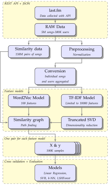
Figure 2: Flow of the data using the methodology described in this work.

3.1 Algorithms

We have evaluated our engineered features with the following models: Linear Regression (LR), Support Vector Machines Regression (SVR) [Smola and Schölkopf, 2004; Gunn et al., 1998], exact and approximate (by means of locality sensitive hashing [Andoni and Indyk, 2006; Bawa et al., 2005]) k-Nearest Neighbors (k-NN) with kernel regression [Terrell and Scott, 1992] to predict new song similarity scores.

Since none of these algorithms work directly with the data returned by the last.fm™ API, we have transformed the data as described in Section 2.1.

As aforementioned, we have used the cosine metric to measure the similarity between songs. Therefore, we define the metric here for completeness. Given two vectors $\vec{x}$ and $\vec{y}$, the similarity between them is defined as the function

$$\mathrm{sim}(\vec{x},\vec{y})=\frac{\sum_{i}x_{i}y_{i}}{\sqrt{\sum_{i}x^{2}_{i}}\sqrt{\sum_{i}y^{2}_{i}}}$$

and, since our feature vectors are composed of non-negative real numbers and without degenerate cases such as vectors with norm equal to zero, this metric will only return values between zero and one.

3.2 Feature Scaling

Feature scaling is needed when using SVM models, as can be confirmed by observing Tables II and III. In that table we see the $R^{2}$ score of how the model performed in the test set for different filtering values in the features and with raw and scaled ($\mu=0$ and $\sigma^{2}=1$). Due to that, we decided to make the whole input have $\mu=0$ and $\sigma^{2}=1$. The parameters obtained for such scaling were done only over the training set, since in practice we will never have access to the whole dataset. Prior to testing the algorithms, though, we used the same parameters found in the training set to scale the test set.

Table II: Effects of feature scaling on the SVM model when executed with the Word2Vec data. Values shown were obtained by running the best cross-validated model against the test set data.

	$R^{2}$ score
	No filtering	similarity > 0.01	similarity > 0.025
Raw	-27.547	-0.825	-0.302
Scaled	-24.610	-0.764	-0.170

Table III: Effects of feature scaling on the SVM model when executed with the tf-idf model. Values shown were obtained by running the best cross-validated model against the test set data.

	$R^{2}$ score
	No filtering	similarity > 0.01	similarity > 0.025
Raw	-13.225	-0.725	-0.164
Scaled	-4.566	-0.490	-0.156

3.3 Support Vector Machine Regression

We implemented a model that uses SVR for prediction [Smola and Schölkopf, 2004]. The model was cross-validated to determine the best parameters using a grid selection model. We evaluated linear and Radial Basis Function (RBF) kernels, varying the regularization constant C between the values $1$, $10$, and $100$ and, for the RBF the $\gamma$ parameter was selected between $0.001$ and $0.0001$.

3.4 k-Nearest Neighbors

The k-NN model is not traditionally a regression model. Therefore, we made a simple adaptation to the algorithm to calculate the similarity between two songs. Once a new query point was submitted, we found the k nearest neighbors and, between these neighbors, computed the mean value of them, and that was the predicted value. The intuition between this heuristic is that songs with similar features will tend to have similar scores.

Table IV: Performance of the k-NN model with the different models and with different number $k$ of neighbors. The best model is shown in bold face.

	$R^{2}$ score
	1 neighbor	5 neighbors	10 neighbors
Word2Vec raw	0.061	0.273	0.271
Word2Vec $s>1\%$	0.239	0.177	0.158
Word2Vec $s>2.5\%$	0.146	0.084	0.085
Tf-idf raw	0.322	0.296	0.410
Tf-idf $s>1\%$	0.166	0.251	0.235
Tf-idf $s>2.5\%$	0.202	0.155	0.175

3.5 Linear Regression

Linear regression is one of the simplest machine learning algorithms that most often than not deliver good results. The algorithm minimizes the residual sum of least squares between the observed responses in the dataset and the responses predicted by linear regression. Due to this simplicity, this is a model that must be evaluated. For if it can explain the data, Occam’s razor determines it should be selected as a good model.

Table V: Performance of the linear regression model.

	$R^{2}$ score	Accuracy
Word2Vec raw	-0.010	0.000 (+/- 0.084)
Word2Vec $s>1\%$	-0.018	-0.023 (+/- 0.020)
Word2Vec $s>2.5\%$	-0.014	-0.032 (+/- 0.060)
Tf-idf raw	0.012	-0.193 (+/- 0.414)
Tf-idf $s>1\%$	0.024	0.015 (+/- 0.032)
Tf-idf $s>2.5\%$	-0.005	-0.038 (+/- 0.097)

3.6 Approximate k-NN with Locality Sensitive Hashing

Building Locality Sensitive Hashing (LSH) forests [Bawa et al., 2005] is an alternative when one is willing to trade accuracy for speed when doing nearest neighbors search. Since we are already implementing k-NN, it seems appropriate to evaluate this algorithm as well, especially considering that nearest neighbors search can become slow in problems of high dimensionality. The performance of the LSH models is summarized in Table VI.

4 Related Work

Eck et al. [2008] use a set of boosted classifiers to map audio features onto tags collected from the Web. Due to the nature of their classifier, it uses the objective approach and, therefore, need the actual audio files, which we are not using. Berenzweig et al. [2004] survey various music-similarity measures and concludes that measures derived from co-occurrence in personal music collections are the most useful ground truth metrics from those evaluated. Aucouturier and Pachet [2002] define a song similarity measure based on the analysis of songs’ timbres, and also evaluate their metric. Johnson [2014] proposes a matrix factorization method that works well for data with implicit feedback, such as song listening patterns.

Table VI: Performance of the LSH model with the different models and with different number $k$ of neighbors. The best model is shown in bold face.

	$R^{2}$ score for number of neighbors
	1	5	10
Word2Vec raw	0.296	0.189	0.305
Word2Vec $s>1\%$	0.234	0.133	0.167
Word2Vec $s>2.5\%$	0.105	0.096	0.069
Tf-idf raw	-0.092	0.261	0.301
Tf-idf $s>1\%$	0.211	0.172	0.154
Tf-idf $s>2.5\%$	0.042	0.097	0.074

5 Evaluation

We have evaluated our system by sampling the information of 100.000 (a hundred thousand) songs from our dataset. This was needed, since the full dataset wouldn’t fit the modest computers we had access to. This set was further divided into two: a training test (which was also used for cross-validation) and a test set, for evaluating the models’ final performance.

In the initial phases of this work we had though about using the Root Mean Squared Error (RMSE) function, defined below, for model performance, but recall all similarity values are between zero and one. Therefore, it would be hard to get an intuitive feel of the model performance.

$$\mathrm{RMSE}(y,\hat{y})=\sqrt{\frac{\sum_{i=1}^{n}{{(\hat{y}_{i}-y_{i})}^{2}}}{n}}$$

Because of the previous discussion, we have decided to evaluate our models using the coefficient of determination ($R^{2}$) score. The $R^{2}$ score is defined below and its value is $1$ when the model can perfectly explain the data and get only deviate below one. Notice that this allows the score to be negative. Therefore, the more negative the $R^{2}$ score, the worse the model. Another advantage of using $R^{2}$ is that, by definition, the $R^{2}$ score of a predictor that always outputs the mean value of the dataset is zero. From that it follows that models with $R^{2}$ values smaller than zero are not that useful.

$$\mathrm{R^{2}}(y,\hat{y})=1-\frac{\sum{{(y_{i}-\hat{y}_{i})}^{2}}}{\sum{{(y_{i}-\bar{y})}^{2}}}$$

The results of the evaluation of the various models used in this work are shown in Tables II–VI. As can be gathered, the best models were the ones based on the nearest neighbors models. Also, notice that they perform significantly better than the predictor of the mean. More striking is that the best results are found when the raw unfiltered data is used, which is the exact opposite of the observed behavior of the SVR model. The linear model stands between the SVR (the worse) and the k-NN models (the best), but it yields values too close to 0 to be particularly useful, and a predictor that predicts the mean value of the data might be better.

6 Conclusion

We have explored machine learning techniques for learning similarity between songs. Particularly, we explored two different methods from the NLP field for building feature matrices that were fed into the algorithms. Of these two methods, the tf-idf one seems to give better results while also executing faster than the Word2Vec one. We also selected models by means of cross-validation, splitting the data into a training and testing set, saving the testing set only for the final evaluation.

About the learning algorithms themselves, it is interesting to notice that an algorithm that generally performs very well in classification tasks (SVR) had the worst performance with our dataset. More interesting is that a relatively simple algorithm (k-NN) that computes the mean of the query point’s neighbors had performance much better than not only than the other algorithms, but also of the estimator based on the mean (with $R^{2}$ score zero).

7 Lessons learned

Most of the effort in preparing this paper was done in understanding and adapting inconsistencies in the data obtained from the last.fm™ API. Also, although data is abundant, and even though this is probably not considered big data, the data is big enough to not fit in commodity computers. Still, the lessons learned in this work allow for one approach for building the base of recommendation systems.

References

- Andoni and Indyk [2006] Alexandr Andoni and Piotr Indyk. Near-optimal hashing algorithms for approximate nearest neighbor in high dimensions. In Foundations of Computer Science, 2006. FOCS’06. 47th Annual IEEE Symposium on, pages 459–468. IEEE, 2006.
- Aucouturier and Pachet [2002] Jean-Julien Aucouturier and Francois Pachet. Music similarity measures: What’s the use? In ISMIR, 2002.
- Bawa et al. [2005] Mayank Bawa, Tyson Condie, and Prasanna Ganesan. Lsh forest: self-tuning indexes for similarity search. In Proceedings of the 14th international conference on World Wide Web, pages 651–660. ACM, 2005.
- Berenzweig et al. [2004] Adam Berenzweig, Beth Logan, Daniel PW Ellis, and Brian Whitman. A large-scale evaluation of acoustic and subjective music-similarity measures. Computer Music Journal, 28(2):63–76, 2004.
- Eck et al. [2008] Douglas Eck, Paul Lamere, Thierry Bertin-Mahieux, and Stephen Green. Automatic generation of social tags for music recommendation. In Advances in neural information processing systems, pages 385–392, 2008.
- Gunn et al. [1998] Steve R Gunn et al. Support vector machines for classification and regression. ISIS technical report, 14, 1998.
- Johnson [2014] Christopher C Johnson. Logistic matrix factorization for implicit feedback data. Advances in Neural Information Processing Systems, 27, 2014.
- Linden et al. [2003] G. Linden, B. Smith, and J. York. Amazon.com recommendations: item-to-item collaborative filtering. IEEE Internet Computing, 7(1):76–80, Jan 2003. ISSN 1089-7801. doi: 10.1109/MIC.2003.1167344.
- Mikolov et al. [2013] Tomas Mikolov, Kai Chen, Greg Corrado, and Jeffrey Dean. Efficient estimation of word representations in vector space. arXiv preprint arXiv:1301.3781, 2013.
- Smola and Schölkopf [2004] Alex J Smola and Bernhard Schölkopf. A tutorial on support vector regression. Statistics and computing, 14(3):199–222, 2004. doi: 10.1023/B:STCO.0000035301.49549.88. URL http://dx.doi.org/10.1023/B:STCO.0000035301.49549.88.
- Terrell and Scott [1992] George R Terrell and David W Scott. Variable kernel density estimation. The Annals of Statistics, pages 1236–1265, 1992.