Min-Max Design of Feedback Quantizers for Netorwked Control Systems

Abstract

In a networked control system, quantization is inevitable to transmit control and measurement signals. While uniform quantizers are often used in practical systems, the overloading, which is due to the limitation on the number of bits in the quantizer, may significantly degrade the control performance. In this paper, we design an overloading-free feedback quantizer based on a $\Delta\Sigma$ modulator, composed of an error feedback filter and a static quantizer. To guarantee no-overloading in the quantizer, we impose an $l_{\infty}$ norm constraint on the feedback signal in the quantizer. Then, for a prescribed $l_{\infty}$ norm constraint on the error at the system output induced by the quantizer, we design the error feedback filter that requires the minimum number of bits that achieves the constraint. Next, for a fixed number of bits for the quantizer, we investigate the achievable minimum $l_{\infty}$ norm of the error at the system output with an overloading-free quantizer. Numerical examples are provided to validate our analysis and synthesis.

I Introduction

In a networked (or distributed) control system, multiple geographically distributed systems exchange their information to achieve control tasks. For example, sensors at a controlled plant send their observation signals to a controller, and the controller transmits control signals to actuators at the plant through communication channels (e.g., see [1] and the reference therein).

If distributed systems are connected by reliable communication channels, then a sufficient level of accuracy of data transmission can be assured. However, it is often the case that communication rates are limited due to physical constraints especially when wireless communication is used. To transmit signals over rate-limited digital communication channels, the continuous-valued (or even discrete-valued) signals have to be quantized into low-resolution signals. When only a small number of bits can be assigned to represent the signals, quantization errors may cause serious degradation in the stability and control performance. This motivates the research on control under limited data rates.

The minimum data rate to keep the state of a closed-loop system in a bounded region with state feedback control has been provided in [2]. Stabilizability and observability under a communication constraint has been studied in [3] for discrete-time, linear and time-invariant (LTI) systems. In [3], a sufficient and necessary condition on the information rate for asymptotic stabilizability and observability has also been presented. The same condition has been shown in [4] for a sufficient and necessary condition for exponentially stabilizability of discrete-time LTI systems with random initial values. The discussions on the minimum data rate based on the information theory gives valuable insights into control under limited data rates. However, even if the rate is assured, the closed-loop system cannot be always stabilized in practice, since the minimum data rate is not a constant rate for each time slot but an averaged rate over time. Also, the rate is evaluated under the ideal assumption that the channel from the controller to the plant has infinite precision and the quantizer has an infinite range for its input. Moreover, the minimum rate is attained by a very complicated quantizer that is hard to implement. In practice, the control signal should be bounded in a fixed range due to physical requirements, only a finite number of bits can be assigned, and the quantizer has a limited range. Taking account of these limitations, we develop an implementable quantizer that requires only a small number of bits for quantization to attain requirements on control performance.

Quantization with error feedback has been originally developed to reduce quantization error in the coefficients of digital filters [5, 6, 7], where the quantization error of a static uniform quantizer is filtered by an error feedback filter and then it is fed back to the input to the static uniform quantizer (see Fig. 4 in Section II). On the other hand, $\Delta\Sigma$ modulators also employ the error feedback mechanism, and are often utilized in practice to convert real numbers into fixed-point numbers [8], since they can be implemented at a relatively low cost.

For networked control systems, a variant of $\Delta\Sigma$ modulator has been studied in [9], which is called a dynamic quantizer. The parameters in the dynamic quantizer can be obtained by linear programming [10] and by convex optimization [11]. To avoid overloading, [10] proposes to limit the $l_{\infty}$ norm of the feedback signals. However, the dynamic quantizer only supports a smaller set of error feedback filters than conventional $\Delta\Sigma$ modulators and hence the optimal performance cannot be guaranteed [12].

Recently, $H_{\infty}$ optimal design of error feedback filters has been proposed based on the generalized Kalman-Yakubovich-Popov lemma [13, 14]. Also, a post filter connected to the $\Delta\Sigma$ modulator is incorporated into the design of the error feedback filter [15] and the weighted noise spectrum is also exploited [16]. In [17], under the assumption that the output of the static uniform quantizer is a white noise, the optimal error feedback filter has been synthesized such that it minimizes the variance of the quantization error subject to the constraint on the variance of the input to the static uniform quantizer. However, the constraint on the variance does not necessarily guarantee no-overloading in the quantizer. In practical control systems such as nuclear plants, an overloading may cause instability followed by a catastrophic accident. To assure that no overloading occurs, we should take into account the maximum absolute value, i.e., the $l_{\infty}$ norm of the input to the quantizer.

This paper develops a quantizer with error feedback that needs a small number of bits required for quantization to achieve the requirement on the worst-case error in the control output, while keeping no-overloading in the quantizer. We regulate the $l_{\infty}$ norm of the feedback signals in the quantizer to assure no-overloading. In our preliminary conference paper [18], the IIR feedback filter is adopted to minimize the $l_{\infty}$ norm of the error at the output under the constraint on the $l_{\infty}$ norm of the feedback signals. In the study of [18], an upper bound of the $l_{\infty}$ norm, which is not tight, was utilized, since the exact $l_{\infty}$ norm of an IIR filter is not easily evaluated. Alternatively, we here adopt FIR feedback filters since the $l_{\infty}$ norm of an FIR filter can be exactly and directly evaluated. We formulate the design of the optimal FIR feedback filter as linear programming, which can be readily solved numerically. The minimum number of bits assigned to the quantizer is determined with the optimized feedback filters. As illustrated by our numerical results, the optimized FIR feedback filter show a better performance than the IIR feedback filter proposed in [18]. Next, for a given number of bits for the quantizer, we investigate the achievable minimum $l_{\infty}$ norm of the error at the system output induced by the quantizer with an overloading-free quantizer. This can be enabled by finding the relationship between $l_{\infty}$ norm of the feedback signal and the $l_{\infty}$ norm of the error in the output, which can be obtained by solving convex optimization problems. Numerical examples are provided to validate our analysis and synthesis.

This paper is organized as follows. Networked systems and quantization are reviewed in Section II. Then, quantizers are synthesized in Section III based on the $l_{\infty}$ norm of the effect of the quantization error and the output of the error feedback filter. Section IV presents numerical results on our synthesis and Section V concludes this paper.

Notation

$\mathbb{Z}$, $\mathbb{R}$, and $\mathbb{R}_{+}$ stand for the set of real numbers, integers, and non-negative real numbers, respectively. The $\mathrm{z}$ transform of a sequence $f=\{f_{k}\}_{k=0}^{\infty}$ is denoted as $F[\mathrm{z}]=\sum_{k=0}^{\infty}f_{k}\mathrm{z}^{-k}$. The output sequence $h$ of an linear and time-invariant (LTI) system $F[\mathrm{z}]$ with the input sequence $g$ (i.e. $h=f\ast g$ where $\ast$ denotes the convolution) is expressed as $h=F[\mathrm{z}]g$. The $l_{\infty}$ norm of a scalar-valued sequence $x=\{x_{k}\}$ is defined as $||x||_{\infty}=\max_{k}|x_{k}|$.

II Error Feedback Quantizer

Figure 1: Feedback control system.

Fig. 1 depicts a feedback control system, in which the plant is assumed to be linear and time-invariant (LTI), and the signals $y$ and $u$ are functions of time in general. Based on the observation signal $y$ from the plant, the controller generates the control input $u$ to the plant.

Figure 2: Control system with quantization.

The observation signal $y$ and the control input $u$ are assumed to be transmitted through digital communication channels. If $y$ and $u$ are real-valued signals, quantization is required to convert them into discrete-valued signals before transmission as illustrated in Fig. 2. Note that even if $y$ and $u$ are discrete-valued digital signals, they may have to be rounded off when the capacities of the communication channels are limited.

The difference between the input and the output of the quantizer is called the quantization error. There are two quantization errors; one is the quantization error denoted by $e_{c}$ for the control signal $u$ and the other is the quantization error $e$ for the observation signal $y$. With these quantization errors, the control system in Fig. 2 can be modeled by an additive-noise control system shown in Fig. 3.

Controllers are often connected to plants through wired networks. On the other hand, the observation signal are collected by sensors, which may be connected through wireless networks. Thus, we here focus on the quantization error $e$ of the observation signal, assuming that there is no quantization error at the controller. We also assume that each sensor observes a scalar-valued signal to be quantized and works independently of the other sensors. Since we consider the independent quantization of each entries of $y$, we assume $y$ to be a scalar-valued signal to a particular quantizer for simplicity of presentation. We also assume the plant is a single-input and single-output (SISO) system. Note that, most of our results may be applied to the quantization error at the controller and the multiple-input and multiple-output (MIIMO) systems. We assume the reachability and the observability of the plant, without which the plant cannot be stabilized in general.

Figure 3: Control system and quantization error signals.

In quantization, real numbers are mapped into their binary representation. Fixed-point representation and floating-point representation are available for quantization. In this paper, we take fixed-point representation into account since it is often adopted in embedded systems.

Let us take a static uniform quantizer for example. The static uniform quantizer can be described by two parameters, the quantization interval $d\in\mathbb{R}_{+}$ and the saturation level $L\in\mathbb{R}_{+}$. For simplicity, we assume that $L$ is an integer multiple of $d$. For the static quantizer, let us consider a mid-rise quantizer $Q(\xi)$ expressed as

$$Q(\xi)=\left\{\begin{array}[]{ll}\left(i+\frac{1}{2}\right)d,&|\xi|\leq L+\frac{d}{2}\\ &\quad\quad\mbox{~{}~{}and~{}~{}}\xi\in[id,(i+1)d),i\in{\mathbb{Z}}\\ L,&\xi>L+\frac{d}{2}\\ -L,&\xi<-L-\frac{d}{2}\\ \end{array}\right.$$ (1)

The overloading is the saturation due to the fixed number of bits to represent the quantized values in binary. For the mid-rise quantizer, the overloading occurs if $|\xi|>L+\frac{d}{2}$.

The static uniform quantizer is often utilized in practice but its errors and effects of the overloading are not negligible unless a sufficient number of bits is assigned to the quantizer. To mitigate these influences, we adopt a quantizer with an error feedback filter, which has been originally developed to reduce the effects of the quantized coefficients in digital filters [5, 6, 7].

Figure 4: Error feedback quantizer.

Fig. 4 illustrates a block diagram of our quantizer. The quantization error, or the round-off error, of the static uniform quantizer $Q(\cdot)$ is defined as

$$w_{k}=v_{k}-\xi_{k},\quad k=0,1,2,\ldots$$ (2)

where $\xi_{k}$ and $v_{k}$ are respectively the input and the output vectors of the static uniform quantizer at time $k$. Note that the round-off error $w$ of the static quantizer is different from the quantization error defined as

$$e=v-y.$$ (3)

The round-off error signal $w$ is filtered by the error feedback filter $R[\mathrm{z}]-1$ and then it is fed back to the input to the quantizer. The error feedback filter $R[\mathrm{z}]-1$ has to be strictly proper, that is, $R[\infty]=1$. The quantizer in Fig. 4 is also known as a $\Delta\Sigma$ modulator, which is an efficient analog to digital (A/D) converter with feedback from the output of a static uniform quantizer to shape the quantization noise [8]. In the $\Delta\Sigma$ modulator, $R[\mathrm{z}]$ is called a noise shaping filter or a noise transfer function.

The input signal $\xi$ to the static quantizer can be expressed from Fig. 4 as

$$\xi=y+(R[\mathrm{z}]-1)w.$$ (4)

From (2) and (4), the quantization error $e$ is given by

$$e=v-y=R[\mathrm{z}]w.$$ (5)

Thus, the output signal of the quantizer can be expressed as

$$v=y+e=y+R[\mathrm{z}]w.$$ (6)

Let the output signal of interest be $z$ and the transfer function from $y$ to $z$ be $H[\mathrm{z}]$. Then, since the plant is assumed to be reachable and observable, there exists a controller that stabilizes the control system when there is no quantization error. With this controller, $H[\mathrm{z}]$ is stable. Thus, without loss of generality, we can assume that $H[\mathrm{z}]$ is stable.

Since $e$ also goes through $H[\mathrm{z}]$, the error signal in $z$ that comes from the quantization error $e$ can be expressed as

$$\epsilon=H[\mathrm{z}]e=H[\mathrm{z}]R[\mathrm{z}]w.$$ (7)

Unless $H[\mathrm{z}]R[\mathrm{z}]=0$, we cannot assure that $\epsilon_{k}\rightarrow 0$ as $k\rightarrow\infty$ due to the unpredictable round-off errors. Thus, we cannot guarantee the exponential stability of the feedback system, even if $H[\mathrm{z}]$ is stable. All we can do is to mitigate the effect of the quantization given by (7). Thus, our goal is to design an error feedback quantizer so that the maximum absolute value of $\epsilon$ is not greater than a prescribed threshold $\gamma_{\epsilon}$, which can be expressed as

$$\max_{k}|\epsilon_{k}|\leq\gamma_{\epsilon}$$ (8)

or equivalently as

$$||\epsilon||_{\infty}\leq\gamma_{\epsilon}.$$ (9)

III Synthesis of Error Feedback Quantizer

Unless overloading occurs, the round-off error $w$ is bounded such as

$$||w||_{\infty}\leq\frac{d}{2}.$$ (10)

Otherwise, the signal $z$ of interest cannot be bounded in general, since $w$ may be unbounded due to overloading. Then, the overloading complicates the control law, since $||\epsilon||_{\infty}$ depends on it. To design the controller and the quantizer independently, it is better to avoid the overloading in the static uniform quantizer.

If there is no overloading, then $y$ is bounded, since the system is stable and the error $\epsilon$ is bounded with a stable $R[\mathrm{z}]$. Without loss of generality, we can assume that the observation signal has the symmetric magnitude limitation described as

$$||y||_{\infty}\leq L_{y}.$$ (11)

Let us adopt the static uniform quantizer characterized by (1) in our error feedback quantizer. From our definitions, if the feedback signal $\eta$ meets

$$||y+\eta||_{\infty}\leq L+\frac{d}{2},$$ (12)

then any overloading never happens at the static quantizer.

Let us introduce the norm of a system $F[\mathrm{z}]=\sum_{k=0}^{\infty}f_{k}{\mathrm{z}}^{-k}$ induced by the $l_{\infty}$ norm of the input and output signals defined as [19]

$$||F[\mathrm{z}]||=\sup_{x\neq 0}\frac{||F[\mathrm{z}]x||_{\infty}}{||x||_{\infty}},$$ (13)

for $x\in l_{\infty}$ (i.e. $\|x\|_{\infty}<\infty$). If $F[\mathrm{z}]$ is an SISO system, the norm is equivalent to the $l_{1}$ norm of the impulse response of the system, that is, we have

$$||F[\mathrm{z}]||=\sum_{k=0}^{\infty}|f_{k}|.$$ (14)

It follows from (12) and $||\eta||_{\infty}\leq||R[\mathrm{z}]-1||(d/2)$ that if one sets

$$L_{y}+||R[\mathrm{z}]-1||\frac{d}{2}\leq L+\frac{d}{2}$$ (15)

then no-overloading in the static uniform quantizer is assured. In other words, the $l_{\infty}$ norm of the feedback signal should be equal to or less than $L+d/2-L_{y}$.

For the binary representation of the observation signals, we have to determine its accuracy and range, i.e., the quantization interval $d$ and the saturation level $L$ for the uniform quantizer. If we assign $b$ bits to represent the observation signal, we have

$$2L=(2^{b}-1)d.$$ (16)

From (15) and (16), we summarize the above discussion as a proposition:

Proposition 1.

There is no overloading in the error feedback quantizer composed of an error feedback filter $R[\mathrm{z}]-1$ and a mid-rise quantizer if

$$L_{y}+||R[\mathrm{z}]-1||\frac{d}{2}\leq 2^{b-1}d$$ (17)

where $b$ is the number of bits assigned to the mid-rise quantizer, $d$ and $L_{y}$ denote its quantization interval and saturation level respectively.

Now, we would like to find the number of bits that assures no-overloading under the constraint (9), which is, from (7), achieved if

$$||H[\mathrm{z}]R[\mathrm{z}]||\frac{d}{2}\leq\gamma_{\epsilon}.$$ (18)

To obtain the minimum $b$ that satisfies (17), we set the quantization interval of our static uniform quantizer to be

$$d=\frac{2\gamma_{\epsilon}}{||H[\mathrm{z}]R[\mathrm{z}]||}.$$ (19)

Substituting (19) into (17) leads to

$$\frac{L_{y}}{\gamma_{\epsilon}}||H[\mathrm{z}]R[\mathrm{z}]||+||R[\mathrm{z}]-1||\leq 2^{b}.$$ (20)

For given $L_{y}$ and $\gamma_{\epsilon}$, the left hand side of the inequality above can be evaluated with $||H[\mathrm{z}]R[\mathrm{z}]||$ and $||R[\mathrm{z}]-1||$, whose minimum can be obtained by solving the following optimization problem:

$$\min_{R[\mathrm{z}]\in RH_{\infty},\gamma_{\epsilon}}c\tilde{\gamma}_{\epsilon}+\tilde{\gamma}_{\eta}$$ (21)

subject to $R[\infty]=1$ and

$$||H[\mathrm{z}]R[\mathrm{z}]|| \leq\tilde{\gamma}_{\epsilon}$$ (22)

$$||R[\mathrm{z}]-1|| \leq\tilde{\gamma}_{\eta}$$ (23)

where $RH_{\infty}$ is the set of stable proper rational functions with real coefficients and

$$c=\frac{L_{y}}{\gamma_{\epsilon}}.$$ (24)

It should be noted that the objective function is a linear in $\tilde{\gamma}_{\epsilon}$ and $\tilde{\gamma}_{\eta}$.

The problem above can be solved if we restrict $R[\mathrm{z}]$ to have a finite impulse response (FIR). On the other hand, the global optimal solution is not available for general infinite impulse response (IIR) filters.

III-A FIR filter design

If $R[\mathrm{z}]$ is an FIR filter of order $n$, then the problem can be formulated as a linear programming (LP) and be numerically solved as follows.

To solve the problem, we express the composite system $H[\mathrm{z}]R[\mathrm{z}]$ as a state-space realization. We denote the state-space matrices of a state-space realization of $H[\mathrm{z}]$ as $(A_{h},B_{h},C_{h},D_{h})$, while the state-space matrices of a state-space realization of $R[\mathrm{z}]$ as $(A_{r},B_{r},C_{r},D_{r})$ with $D_{r}=1$. Then, the state-space realization of $H[\mathrm{z}]R[\mathrm{z}]$ can be written as

$$x_{k+1} = {\cal A}x_{k}+{\cal B}w_{k}$$ (25)

$$\epsilon_{k} = {\cal C}x_{k}+{\cal D}w_{k}$$ (26)

where the state-space matrices for this are given as

$${\cal A} = \left[\begin{array}[]{cc}A_{r}&B_{r}C_{h}\\ \bm{0}&A_{h}\end{array}\right]$$ (29)

$${\cal B} = \left[\begin{array}[]{c}B_{r}\\ B_{h}\end{array}\right]$$ (32)

$${\cal C} = \left[\begin{array}[]{cc}C_{r}&D_{r}C_{h}\end{array}\right]$$ (34)

$${\cal D} = D_{h}.$$ (35)

The impulse response from $w$ to $\epsilon$ can be expressed as

$$f_{k}=\left\{\begin{array}[]{cc}{\cal D},&k=0\\ {\cal C}{\cal A}^{k-1}{\cal B},&k\neq 0\end{array}\right.$$ (38)

A state-space realization $(A_{r},B_{r},C_{r},1)$ of the FIR filter $R[\mathrm{z}]=1+\sum_{k=1}^{n}r_{k}\mathrm{z}^{-k}$ is given by

$$A_{r} =\begin{bmatrix}0&1&0&\cdots&0\\ \vdots&\ddots&\ddots&\ddots&\vdots\\ \vdots&&\ddots&\ddots&0\\ \vdots&&&\ddots&1\\ 0&\cdots&\cdots&\cdots&0\\ \end{bmatrix},\ B_{r}=\begin{bmatrix}0\\ \vdots\\ 0\\ 1\\ \end{bmatrix}$$ (39)

$$C_{r} =\begin{bmatrix}r_{n},&r_{n-1},&\cdots&r_{1}\end{bmatrix},D_{r}=1.$$ (40)

Since $A_{r}$ and $B_{r}$ are constant, ${\cal A}$, ${\cal B}$, and ${\cal D}$ are constant. Moreover, ${\cal A}$ is Shur, that is, all eigenvalues of ${\cal A}$ are strictly inside the unit circle, since $H[\mathrm{z}]$ is stable.

For a sufficiently large integer $m$, we can approximate $||H[\mathrm{z}]R[\mathrm{z}]||$ such that

$$||H[\mathrm{z}]R[\mathrm{z}]||=|D_{h}|+\sum_{k=1}^{m}|{\cal C}{\cal A}^{k-1}{\cal B}|.$$ (41)

Then, our problem can be expresses as the following minimization problem:

$$\min_{r_{1},\ldots,r_{n}}c\tilde{\gamma}_{\epsilon}+\tilde{\gamma}_{\eta}$$ (42)

subject to

$$|D_{h}|+\sum_{k=1}^{m}|{\cal C}{\cal A}^{k-1}{\cal B}| \leq\tilde{\gamma}_{\epsilon}$$ (43)

$$\sum_{k=1}^{n}|r_{k}| \leq\tilde{\gamma}_{\eta}.$$ (44)

Note that the matrix ${\cal C}$ depends linearly on $r_{1},\ldots,r_{n}$ as in (34) and (40).

Introducing non-negative auxiliary variables $\bar{f}_{k}$ for $k=1,\ldots,m$, one can express (43) as

$$\sum_{k=1}^{m}\bar{f}_{k}\leq\tilde{\gamma}_{\epsilon}$$ (45)

$$-\bar{f}_{k}\leq|D_{h}|+{\cal C}{\cal A}^{k-1}{\cal B}\leq\bar{f}_{k}\quad\mbox{for}\quad k=1,\ldots,m$$ (46)

Similarly, with non-negative auxiliary variables $\bar{r}_{k}\geq 0$ for $k=1,\ldots,n$, (44) is equivalent to

$$\sum_{k=1}^{n}\bar{r}_{k}\leq\tilde{\gamma}_{\eta}$$ (47)

$$-\bar{r}_{k}\leq r_{k}\leq\bar{r}_{k}\quad\mbox{for}\quad k=1,\ldots,n.$$ (48)

Then, our minimization problem is formulated as the following linear programming (LP):

$$\min_{r_{1},\ldots,r_{n},\bar{f}_{1},\ldots,\bar{f}_{m},\bar{r}_{1},\ldots,\bar{r}_{n},}c\tilde{\gamma}_{\epsilon}+\tilde{\gamma}_{\eta}$$ (49)

subject to (45), (46), (47), (48), and

$$\bar{f}_{k}\geq 0\quad\mbox{for}\quad k=1,\ldots,m$$ (50)

$$\bar{r}_{k}\geq 0\quad\mbox{for}\quad k=1,\ldots,n.$$ (51)

III-B IIR filter design

Let us shortly introduce the IIR filter design proposed in [18], where the order of $R[\mathrm{z}]$ is set to be equal to the order of $H[\mathrm{z}]$. For the design of IIR filters, we re-express the state-space realization of $H[\mathrm{z}]R[\mathrm{z}]$ as

$${\cal A} = \left[\begin{array}[]{cc}A_{h}&B_{h}C_{r}\\ \bm{0}&A_{r}\end{array}\right]$$ (54)

$${\cal B} = \left[\begin{array}[]{c}B_{h}\\ B_{r}\end{array}\right]$$ (57)

$${\cal C} = \left[\begin{array}[]{cc}C_{h}&D_{h}C_{r}\end{array}\right].$$ (59)

In [20], the following lemma has been provided by using the invariant set of a discrete-time system.

Lemma 1.

Suppose the initial state $x_{0}$ is $0$ and the input $w$ is bounded as $||w||_{\infty}\leq 1$. Then, the state vectors $x_{k},k=1,2,\ldots$ remain in the ellipsoid

$${\cal E}({\cal P})=\{x:x^{T}{\cal P}x\leq 1\}$$ (60)

if and only if there exist a scalar $\alpha\in[0,1-\rho^{2}({\cal A})]$ and a positive definite matrix ${\cal P}$ satisfying

$$\left[\begin{array}[]{ccc}(1-\alpha){\cal P}&\bm{0}&{\cal A}^{T}{\cal P}\\ \bm{0}&\alpha&{\cal B}^{T}{\cal P}\\ {\cal P}{\cal A}&{\cal P}{\cal B}&{\cal P}\end{array}\right]\succeq\bm{0},$$ (61)

where $\rho(A)$ is the spectrum radius of $A$.

It follows from $\epsilon_{k}={\cal C}x_{k}+D_{h}w_{k}$ that if $x_{k}\in{\cal E}({\cal P})$, then

$$\sup_{x_{k}\in{\cal E}(P)}|\epsilon_{k}-D_{h}w_{k}|^{2}\leq\operatorname{trace}\left({\cal C}{\cal P}^{-1}{\cal C}^{T}\right).$$ (62)

Thus, we have

$$||\epsilon||_{\infty}\leq|D_{h}|\frac{d}{2}+\left[\operatorname{trace}\left({\cal C}{\cal P}^{-1}{\cal C}^{T}\right)\right]^{\frac{1}{2}}.$$ (63)

On the other hand, with

$$\tilde{{\cal C}}=\left[\begin{array}[]{cc}\bm{0}&C_{r}\end{array}\right]$$ (64)

we can express $\eta$ as

$$\eta_{k}=\tilde{{\cal C}}x_{k}$$ (65)

which leads to

$$||\eta||_{\infty}\leq\left[\operatorname{trace}\left(\tilde{{\cal C}}{\cal P}^{-1}\tilde{{\cal C}}^{T}\right)\right]^{\frac{1}{2}}.$$ (66)

Unlike FIR filters, we cannot analytically evaluate $||\epsilon||_{\infty}$ and $||\eta||_{\infty}$. Instead, we consider the minimization using the right hand sides of (63) and (66), that is, the upper bounds of $||\epsilon||_{\infty}$ and $||\eta||_{\infty}$, such that:

$$\operatorname{trace}\left({\cal C}{\cal P}^{-1}{\cal C}^{T}\right) \leq\mu_{\epsilon}$$ (67)

$$\operatorname{trace}\left(\tilde{{\cal C}}{\cal P}^{-1}\tilde{{\cal C}}^{T}\right) \leq\mu_{\eta}.$$ (68)

Note that the upper bound of our objective function $c\tilde{\gamma}_{\epsilon}+\tilde{\gamma}_{\eta}$ is given by $c\sqrt{\mu_{\epsilon}}+\sqrt{\mu_{\eta}}$, which is not convex in $\mu_{\epsilon}$ and $\mu_{\eta}$. In stead of directly solving the problem, let us consider the following problem:

$$\min_{R[\mathrm{z}]\in RH_{\infty},x_{k}\in{\cal E}({\cal P}),\mu_{\epsilon}}\mu_{\epsilon}$$ (69)

subject to $R[\infty]=1$, (67) and (68).

The condition $x_{k}\in{\cal E}({\cal P})$ is described by (61), which is a bilinear matrix inequality (BMI) of the variables. On the other hand, by using the Schur complement, (67) and (68) can be expressed as linear matrix inequalities (LMIs):

$$\left[\begin{array}[]{cc}{\cal P}&{\cal C}^{T}\\ {\cal C}&\mu_{\epsilon}\end{array}\right] \succeq\bm{0}$$ (72)

$$\left[\begin{array}[]{cc}{\cal P}&\tilde{{\cal C}}^{T}\\ \tilde{{\cal C}}&\mu_{\eta}\end{array}\right] \succeq\bm{0}.$$ (75)

Since the BMI is not convex, we cannot yet solve (69). Fortunately, we can convert the BMI into an LMI and then, since the LMI is convex, we can solve the minimization problem (69) numerically as detailed in Appendix.

By solving the convex optimization problem (69) for different values for $\mu_{\eta}$, we obtain the optimal IIR feedback filters for different constraints on the $l_{\infty}$ norms of the feedback back signals. With the designed feedback filters $R[\mathrm{z}]-1$, we can evaluate the pair $(||R[\mathrm{z}]-1||,||H[\mathrm{z}]R[\mathrm{z}]||)$ and find the optimal $R[\mathrm{z}]$ that achieves the minimum of the left hand side of (20), which gives the minimum number for $b$.

III-C Minimum $l_{\infty}$ norm for a fixed number of bits

We have investigated the number of bits required for quantization to attain a prescribed requirement on the control performance and the overloading-free quantization at the same time. Now, we would like to consider another problem to find the achievable minimum $l_{\infty}$ norm of the error in the signal of interest with an overloading-free quantizer for a given number of bits.

Suppose that the number of bits assigned to the static quantizer is given and fixed. We would like to design the overloading-free feedback quantizer that minimizes the $l_{\infty}$ norm of the error $\epsilon$. From (17), we obtain

$$L_{y}\leq\left(2^{b-1}-\frac{1}{2}||R[\mathrm{z}]-1||\right)d.$$ (76)

Since $d$ must be positive, we have to meet $||R[\mathrm{z}]-1||<2^{b}$. It follows from $||\epsilon||_{\infty}\leq||H[\mathrm{z}]R[\mathrm{z}]||d/2$ that $||\epsilon||_{\infty}$ is bounded with $d=L_{y}/\left(2^{b-1}-||R[\mathrm{z}]-1||/2\right)$ as

$$||\epsilon||_{\infty}\leq\frac{L_{y}||H[\mathrm{z}]R[\mathrm{z}]||}{2^{b}-||R[\mathrm{z}]-1||}.$$ (77)

It is obvious that for a fixed value of $||R[\mathrm{z}]-1||$, the upper bound for $||\epsilon||_{\infty}$ is minimized by the filter $R[\mathrm{z}]$ that minimizes $||H[\mathrm{z}]R[\mathrm{z}]||$. Then, for a fixed upper bound $\tilde{\gamma}_{\eta}$ of $||R[\mathrm{z}]-1||$, the optimal filter can be found by solving the following optimization problem:

$$\min_{R[\mathrm{z}]\in RH_{\infty},\tilde{\gamma}_{\epsilon}}\tilde{\gamma}_{\epsilon}$$ (78)

subject to $R[\infty]=1$, (22), and (23).

For a fixed upper bound for $||R[\mathrm{z}]-1||$, we have the value for $||H[\mathrm{z}]R[\mathrm{z}]||$ by solving the optimization problem. Then, by solving the problem for different values for $||R[\mathrm{z}]-1||$, the relationship between $||R[\mathrm{z}]-1||$ and $||H[\mathrm{z}]R[\mathrm{z}]||$ can be obtained. Finally, with the values for the pair $(||R[\mathrm{z}]-1||,||H[\mathrm{z}]R[\mathrm{z}]||)$, we can obtain the minimum of the right hand side of (77).

As in Sections III-A and III-B, the problem can be formulated as an LP for FIR $R[\mathrm{z}]$, whereas the upper bounds of the norms have to be evaluated for IIR $R[\mathrm{z}]$. The details are omitted, since the optimization problems can be similarly solved as described in III-A and III-B.

IV Numerical examples

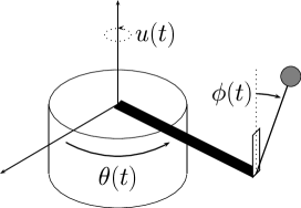
Figure 5: Rotary inverted pendulum.

We here consider the rotary inverted pendulum (see e.g. [1]) depicted in Fig. 5 for our design example.

The pendulum connected at the end of the rotary arm is controlled by rotating the main body in the horizontal plane. The yaw angle of the arm is $\theta(t)$. The pendulum freely swings about a pitch angle $\phi(t)$ in the vertical plane to the arm. The torque $u(t)$ is applied to actuate the pendulum. If $\phi(t)=0$, then the pendulum is balanced in the inverted position.

We define the state of the rotary inverted pendulum as

$$x^{T}(t)=[\phi(t),\theta(t),\dot{\phi}(t),\dot{\theta}(t)].$$ (79)

We periodically change the yaw angle, while keeping the stability of the rotary inverted pendulum. The target value of the yaw angle $\bar{\theta}(t)$ is

$$\bar{\theta}(t)=\left\{\begin{array}[]{ll}\frac{\pi}{2}&(10k\leq t<5+10k)\\ 0&(5+10k\leq t<10(k+1))\end{array}\right.$$ (80)

for $k=0,1,\ldots$. The initial values of the states are assumed to be zero.

We linearize the continuous-time dynamical system of the pendulum and discretize this with the sampling period $T_{s}=0.01$. Let $A,B,C,D$ be the state-space matrices of the linearized and discretized system. Since the continuous-time system is strictly proper, we have $D=0$. The state-space matrices $A$ and $B$ of the discrete-time linearized system are given by

$$A = \left[\begin{array}[]{cccc}1.0056&0&0.0100&0.0001\\ -0.0003&1.0000&-0.0000&0.0100\\ 1.1134&0&1.0056&0.0149\\ -0.0653&0&-0.0003&0.9926\end{array}\right]$$ (85)

$$B = \left[\begin{array}[]{c}-0.0004\\ 0.0002\\ -0.0864\\ 0.0431\end{array}\right].$$ (90)

Assuming that all of the state variables be available at the controller (i.e. $C$ is the identity matrix), we adopt the state feedback control and determined its gain $K$ by the linear quadratic regulator (LQR) technique to minimize

$$\sum_{k=0}^{\infty}\left(x_{k}^{T}Q_{lqr}x_{k}+r|u_{k}|^{2}\right)$$ (91)

where the weights are

$$Q_{lqr}=\operatorname{diag}[10,2,0.5,0],\quad r=0.05.$$ (92)

Our signals of interest is the discretized $\phi(t)$, which is expressed as $\phi_{k}=C_{1}x_{k}$ with

$$C_{1} =\left[\begin{array}[]{cccc}1&0&0&0\end{array}\right].$$ (94)

The transfer function from the $l$th entry of the quantization error $\eta$ to $\phi$ and $\theta$ is found to be $C_{1}(\mathrm{z}I-A-BK)^{-1}BK_{l}$ with $K=[K_{1},K_{2},K_{3},K_{4}]=[57.2598,6.0910,6.2562,3.4953]$.

Now let us design FIR and IIR filters of order 4 for the error feedback. We consider the quantization of $\phi$, the first entry of the state variables, to mitigate the effect of the quantization on $\phi$. The transfer function is given by

$$H[\mathrm{z}] =C_{1}(\mathrm{z}I-A-BK)^{-1}BK_{1}$$ (95)

$$=\frac{0.02475\mathrm{z}^{3}-0.02482\mathrm{z}^{2}-0.02463\mathrm{z}+0.02469}{\mathrm{z}^{4}-3.59\mathrm{z}^{3}+4.808\mathrm{z}^{2}-2.844\mathrm{z}+0.626}$$

whose zeros are $-0.9975$, $1$, and $1$.

The constraint on the maximum absolute value of $\epsilon$ is set to be $\gamma_{\epsilon}=0.05$ and $L_{y}$ in (11) is set to be $\pi/2$.

With the designed optimal FIR feedback filter, the value of the objective function $c||H[\mathrm{z}]R[\mathrm{z}]||+||R[\mathrm{z}]-1||$ is 5.2729. On the other hand, the value with the designed IIR feedback filter is 5.8831. The FIR filter exhibits a better performance than the IIR filter. This is due to the fact that the exact value of the $l_{\infty}$ norm is evaluated for the design of the FIR filter, whereas only an upper bound can be used for the design of the IIR filter. In both cases, the required number of bits is 3 to satisfy the constraint (20), while the conventional static uniform quantizer requires $6$ bits to meet the constraint on $\epsilon$, since $(L_{y}/\gamma_{\epsilon})||H[\mathrm{z}]||=47.788<2^{6}$.

Simulations are conducted with the designed optimal FIR error feedback filter. To clarify the difference, we only quantize the signal $\phi$ of interest.

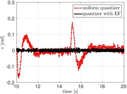
Figure 6: Error of pitch angles of the pendulum controlled with the $3$-bit quantizers having the optimized FIR error feedback filter (solid line) and the conventional uniform quantizers (dash-dotted line).

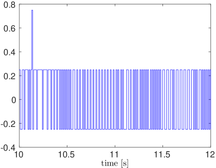
Figure 7: Output of the designed quantizer for pitch angle.

Fig. 6 compares the error signal $\epsilon$ of the pendulum controlled with the $3$-bit quantizers having the optimized FIR error feedback filter (solid line) and the conventional uniform quantizer (dash-dotted line) for $10\leq t<20$. The maximum absolute value of the error for our designed quantizer is less than 0.05, while the maximum absolute value of the error for the conventional uniform quantizers is about 0.18. Our designed quantizer satisfies the requirement on the error clearly outperforms the conventional uniform quantizer.

The output of our designed quantizer for $10\leq t<12$ is shown in Fig. 7. Only three values are taken, which implies that only 2 bits are required in practice, although our analysis suggests 3 bits. This is because we adopt the worst-case error for our performance measure. Indeed, it is well-known that the condition on the maximum of the absolute value of errors leads to conservative results.

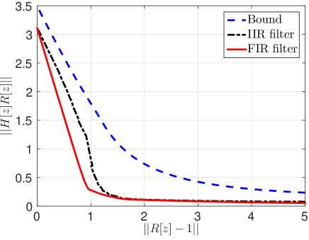
Figure 8: Relation between $||R[\mathrm{z}]-1||$ and $||H[\mathrm{z}]R[\mathrm{z}]||$ for pitch angle $\phi$.

Next, for a fixed number of bits for the quantizer, we evaluate the $l_{\infty}$ norm of the error in the signal of interest with the designed overloading-free quantizer. We solve the optimization problems discussed in Section III-C.

Fig. 8 depicts $||H[\mathrm{z}]R[\mathrm{z}]||$ as a function of $||R[\mathrm{z}]-1||$. In the design of IIR filters, we minimize the upper bound and then the designed filter is not assured to be optimal. Here, $(\sqrt{\mu_{\eta}},\sqrt{\mu_{\epsilon}})$ serves as an upper bound for $(||R[\mathrm{z}]-1||,||H[\mathrm{z}]R[\mathrm{z}]||)$ of IIR filters. On the other hand, in the design of FIR filters, we minimize the objective function directly and the designed filter is optimal among FIR filters. This may be a reason why the designed FIR filters achieve smaller error norm than the designed IIR filers.

As $||R[\mathrm{z}]-1||$ increases from zero, $||H[\mathrm{z}]R[\mathrm{z}]||$ decreases rapidly at first and then floors. It should be remarked that $||R[\mathrm{z}]-1||=0$ implies that there is not any error feedback filter, that is, the quantizer is just a static uniform quantizer.

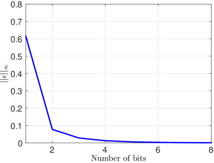
Figure 9: $||\epsilon||_{\infty}$ for different numbers of bits.

From the values of $(||R[\mathrm{z}]-1||,||H[\mathrm{z}]R[\mathrm{z}]||)$ in Fig. 8, we compute the norm $||\epsilon||_{\infty}$ with (14) for different numbers of bits from 1 to 8, which is plotted in Fig. 9. This figure clarifies the relationship between the error norm and the number of bits assigned to the quantizer.

The norm of our quantizer decays exponentially with a rate faster than $1/2$. We may conclude that our quantizer is more efficient in the number of bits than the conventional quantizer without the error feedback filter, since its decay rate of the error norm with respect to the number of bits is given by $1/2$.

V Conclusion

We have studied a feedback quantizer composed of a static quantizer and an error feedback filter. It has been shown that quantizers can be designed independently of the control law. Then, we have investigated the necessary number of bits required for quantization to attain the requirement on the system output, while keeping no-overloading in the quantizer. The number of bits assigned to the quantizer can be obtained by designing the error feedback filter that minimizes a constraint for no-overloading. The design of FIR filters has been formulated as linear programming by directly evaluating the $l_{\infty}$ norm, whereas the design of IIR filters has been as a convex optimization problem by using upper bounds on the $l_{\infty}$ norm. In our design example, if one assigns the same order for filters, the optimized FIR filter exhibits a better performance than the designed IIR filter. The efficiency of the designed quantizer has been demonstrated by simulation.

Appendix A Numerical evaluation based on LMIs

Let us convert the non-convex BMI (61) to an LMI by using the change of variables proposed independently in [21] and [22].

Let the order of $R[\mathrm{z}]$ be equal to the order $n$ of the system $H[\mathrm{z}]$. The set of $n\times n$ positive definite matrices is denoted as $PD(n)$. We define the following matrices $\{P_{f},S_{f},W_{f},W_{g},L\}$, where $P_{f}\in PD(n)$, $S_{f}\in PD(n)$, $W_{f}\in\mathbb{R}^{1\times n}$, $W_{g}\in\mathbb{R}^{n\times 1}$, $L\in\mathbb{R}^{n\times n}$, with $P_{f}$ and $P_{g}$. Let us also define matrices from $\{P_{f},S_{f},W_{f},W_{g},L\}$ as

$${\cal P}^{-1} = \left[\begin{array}[]{cc}P_{f}&S_{f}\\ S_{f}&S_{f}\end{array}\right]$$ (98)

$$U = \left[\begin{array}[]{cc}P_{f}&I_{n}\\ S_{f}&\bm{0}\end{array}\right]$$ (101)

$$P_{g} = (P_{f}-S_{f})^{-1}$$ (102)

and the matrices $\{M_{{\cal A}},M_{{\cal B}},M_{{\cal C}},M_{{\cal P}}\}$ as

$$M_{{\cal A}} =\left[\begin{array}[]{cc}A_{h}P_{f}+B_{h}W_{f}&A_{h}\\ L&P_{g}A_{h}\\ \end{array}\right]$$ (105)

$$M_{{\cal B}} =\left[\begin{array}[]{c}B_{h}\\ W_{g}\end{array}\right]$$ (108)

$$M_{{\cal C}} =\left[\begin{array}[]{cc}C_{h}P_{f}+D_{h}W_{f}&C_{h}\end{array}\right]$$ (110)

$$M_{{\cal P}} =\left[\begin{array}[]{cc}P_{f}&I_{n}\\ I_{n}&P_{g}\\ \end{array}\right]$$ (113)

Direct computations show that if the matrices $\{A_{r},B_{r},C_{r}\}$ are

$$A_{r} =[B_{h}W_{f}-P_{g}^{-1}(L-P_{g}A_{h}P_{f})]S_{f}^{-1}$$ (114)

$$B_{r} =B_{h}-P_{g}^{-1}W_{g}$$ (115)

$$C_{r} =W_{f}S_{f}^{-1}$$ (116)

then $\{{\cal A},{\cal B},{\cal C}\}$ satisfy

$$M_{{\cal A}} = U^{T}{\cal P}{\cal A}U$$ (117)

$$M_{{\cal B}} = U^{T}{\cal P}{\cal B}$$ (118)

$$M_{{\cal C}} = {\cal C}U$$ (119)

$$M_{{\cal P}} = U^{T}{\cal P}U.$$ (120)

Theorem 1 [22] proves that the BMI for the original variables $\{{\cal A},{\cal B},{\cal C},{\cal P}\}$ is equivalent to the LMI for the new variables $\{M_{{\cal A}},M_{{\cal B}},M_{{\cal C}},M_{{\cal P}}\}$ by replacing $\{{\cal P}{\cal A},{\cal P}{\cal B},{\cal C},{\cal P}\}$ with $\{M_{{\cal A}},M_{{\cal B}},M_{{\cal C}},M_{{\cal P}}\}$. Thus, (61) and (72) are converted into

$$\left[\begin{array}[]{ccc}(1-\alpha)M_{{\cal P}}&\bm{0}&M_{{\cal A}}^{T}\\ \bm{0}&\alpha&M_{{\cal B}}^{T}\\ M_{{\cal A}}&M_{{\cal B}}&M_{{\cal P}}\end{array}\right] \succeq\bm{0}$$ (124)

$$\left[\begin{array}[]{cc}M_{{\cal P}}&M_{{\cal C}}^{T}\\ M_{{\cal C}}&\mu_{\epsilon}\end{array}\right] \succeq\bm{0}.$$ (127)

On the other hand, we have

$$\tilde{{\cal C}}U=\left[\begin{array}[]{cc}C_{r}S_{f}&\bm{0}\end{array}\right]=\left[\begin{array}[]{cc}W_{f}&\bm{0}\end{array}\right]:=M_{\tilde{{\cal C}}}.$$ (128)

Premultiplying (75) by $\operatorname{diag}(U^{T},I)$ and postmultiplying (75) by $\operatorname{diag}(U,I)$ results in

$$\left[\begin{array}[]{cc}M_{{\cal P}}&M_{\tilde{{\cal C}}}^{T}\\ M_{\tilde{{\cal C}}}&\mu_{\eta}\end{array}\right]\succeq\bm{0}.$$ (129)

Therefore the minimization problem

$$\min_{P_{f},P_{g},W_{f},W_{g},L,\mu_{\epsilon}}\mu_{\epsilon}$$ (130)

subject to (124), (127), and (129), gives the minimum of the minimization problem (69) for a given $\alpha$.

For a fixed $\alpha$, the minimization problem is a semidefinite program, which can be numerically solved by existing optimization packages, e.g., CVX [23], a package for specifying and solving convex programs. then, the minimum is given by a line search for $\alpha\in(0,\rho^{2}(A_{h}))$.

References

- [1] N. Ploplys, P. Kawka, and A. Alleyne, “Closed-loop control over wireless networks,” IEEE Control Systems, vol. 24, no. 3, pp. 58–71, Jun 2004.
- [2] W. S. Wong and R. W. Brockett, “Systems with finite communication bandwidth constraints. II. stabilization with limited information feedback,” IEEE Transactions on Automatic Control, vol. 44, no. 5, pp. 1049–1053, 1999.
- [3] S. Tatikonda and S. Mitter, “Control Under Communication Constraints,” IEEE Transactions on Automatic Control, vol. 49, no. 7, pp. 1056–1068, Jul. 2004.
- [4] G. N. Nair and R. J. Evans, “Exponential stabilisability of finite-dimensional linear systems with limited data rates,” Automatica, vol. 39, no. 4, pp. 585–593, Apr. 2003. [Online].
- [5] Tran-Thong and B. Liu, “Error spectrum shaping in narrow-band recursive filters,” IEEE Transactions on Acoustics, Speech and Signal Processing, vol. 25, no. 2, pp. 200–203, Apr 1977.
- [6] W. Higgins and D. Munson, “Noise reduction strategies for digital filters: Error spectrum shaping versus the optimal linear state-space formulation,” IEEE Transactions on Acoustics, Speech and Signal Processing, vol. 30, no. 6, pp. 963–973, Dec 1982.
- [7] T. Laakso and I. Hartimo, “Noise reduction in recursive digital filters using high-order error feedback,” IEEE Transactions on Signal Processing, vol. 40, no. 5, pp. 1096–1107, May 1992.
- [8] R. Schreier and G. C. Temes, Understanding Delta-Sigma Data Converters. Wiley-IEEE Press, 2004.
- [9] S. Azuma and T. Sugie, “Optimal dynamic quantizers for discrete-valued input control,” Automatica, vol. 44, no. 2, pp. 396–406, Feb. 2008.
- [10] ——, “Synthesis of optimal dynamic quantizers for discrete-valued input control,” IEEE Transactions on Automatic Control, vol. 53, no. 9, pp. 2064–2075, Oct. 2008.
- [11] K. Sawada and S. Shin, “Dynamic quantizer synthesis based on invariant set analysis for SISO systems with discrete-valued input,” in the 19th International Symposium on Mathematical Theory of Networks and Systems, 2010, pp. 1385–1390.
- [12] S. Ohno and M. R. Tariq, “Optimization of noise shaping filter for quantizer with error feedback,” IEEE Transactions on Circuits and Systems I: Regular Papers, vol. PP, no. 99, pp. 1–13, 2016.
- [13] M. Nagahara and Y. Yamamoto, “Frequency domain min-max optimization of noise-shaping delta-sigma modulators,” IEEE Transactions on Signal Processing, vol. 60, no. 6, pp. 2828–2839, June 2012.
- [14] X. Li, C. B. Yu, and H. Gao, “Design of delta–sigma modulators via generalized Kalman–Yakubovich–Popov lemma,” Automatica, vol. 50, no. 10, pp. 2700–2708, 2014.
- [15] S. Callegari and F. Bizzarri, “Output filter aware optimization of the noise shaping properties of modulators via semi-definite programming,” IEEE Transactions on Circuits and Systems I: Regular Papers, vol. 60, no. 9, pp. 2352–2365, Sept 2013.
- [16] ——, “Noise weighting in the design of modulators (with a psychoacoustic coder as an example),” IEEE Transactions on Circuits and Systems II: Express Briefs, vol. 60, no. 11, pp. 756–760, Nov 2013.
- [17] M. Derpich, E. Silva, D. Quevedo, and G. Goodwin, “On optimal perfect reconstruction feedback quantizers,” IEEE Transactions on Signal Processing, vol. 56, no. 8, pp. 3871–3890, Aug 2008.
- [18] S. Ohno, M. R. Tariq, and M. Nagahara, “Min-max IIR filter design for feedback quantizers,” submitted to EUSIPCO 2017, Feb. 2017.
- [19] V. Chellaboina, M. Haddad, D. Bernstein, and D. Wilson, “Induced convolution operator norms for discrete-time linear systems,” in Proceedings of the 38th IEEE Conference on Decision and Control, 1999., vol. 1, 1999, pp. 487–492 vol.1.
- [20] H. Shingin and Y. Ohta, “Optimal invariant sets for discrete-time systems: Approximation of reachable sets for bounded inputs,” in 10th IFAC/IFORS/IMACS/IFIP Symposium on Large Scale Systems: Theory and Applications (LSS), 2004, pp. 401–406.
- [21] C. Scherer, P. Gahinet, and M. Chilali, “Multiobjective output-feedback control via LMI optimization,” IEEE Transactions on Automatic Control, vol. 42, no. 7, pp. 896–911, Jul 1997.
- [22] I. Masubuchi, A. Ohara, and N. Suda, “LMI-based controller synthesis: A unified formulation and solution,” International Journal of Robust and Nonlinear Control, vol. 8, no. 8, p. 669–686, July 1998.
- [23] M. Grant and S. Boyd, “CVX: Matlab software for disciplined convex programming, version 2.0 beta,” http://cvxr.com/cvx, Sep. 2012.