Infinite Structured Sparse Factor Analysis

Abstract

Matrix factorisation methods decompose multivariate observations as linear combinations of latent feature vectors. The Indian Buffet Process (IBP) provides a way to model the number of latent features required for a good approximation in terms of regularised reconstruction error. Previous work has focussed on latent feature vectors with independent entries. We extend the model to include nondiagonal latent covariance structures representing characteristics such as smoothness. This is done by . Using simulations we demonstrate that under appropriate conditions a smoothness prior helps to recover the true latent features, while denoising more accurately. We demonstrate our method on a real neuroimaging dataset, where computational tractability is a sufficient challenge that the efficient strategy presented here is essential.

1 Introduction

Matrix factorisation methods decompose multivariate observations into linear combinations of latent features. Consider a $(T\times V)$ data matrix $\mathbb{Y}$ comprising $T$ observations of $V$ dimensional vectors, which is decomposed into a linear combinations of $K$ features as:

$$\mathbb{Y}_{(T\times V)}=\mathbb{W}_{(T\times K)}\mathbb{S}_{(K\times V)}+\mathbb{E}_{(T\times V)}$$ (1)

Dimension reduction can then be effected by approximating $\mathbb{Y}$ with $\mathbb{W}\mathbb{S}$, thus using a smaller number of variables. Here $\mathbb{E}$ is the difference between the low rank approximation and the data, whose sum of squares is the reconstruction error. We will refer to the entries of matrices playing the role of $\mathbb{W}$ as weights and rows of $\mathbb{S}$ as features. A family of methods can be placed within this algebraic structure, including Principal Components Analysis (PCA), Factor Analysis (FA), Independent Components Analysis (ICA) and Non-negative Matrix Factorisation (NMF).

When applying matrix decomposition we generally face uncertainty about the number of latent features, $K$, required to explain the data. We start from the assumption that the reader wishes to learn the latent features, their weights and their number from the data in a single, coherent model for approximating the data. Due to the wide family of methods which conform to the algebraic structure in (1) methods which improve our accounting for dimensional uncertainty have a broad scope for application. At the same time we seek decompositions with desirable characteristics, such as sparse activation of features, or constraints on the covariance structure of latent features.

A previous approach to accounting for uncertainty in $K$ was proposed by Viroli (2009). In that scheme the weights assigned to feature vectors were draws from Gaussian mixture models, while the dimension $K$ was sampled through reversible jump MCMC (RJMCMC). Such a model implies that the representation of observations with respect to the latent features would be dense.

We will primarily be concerned with observations that are natural images. Work on natural images (Hyvärinen et al. (2009)), together with successes in signal processing (Elad et al. (2010)) and representation learning (Bengio et al. (2013)) suggests that modelling representations of images as sparse with respect to a basis is a powerful and parsimonious strategy. In the formalism of (1) this means $\mathbb{W}$ being sparse when $\mathbb{S}$ was chosen appropriately. Hence the approach in Viroli (2009) would not be entirely satisfying as a model for natural images.

An alternate strategy to account for uncertainty in $K$ was proposed by Knowles and Ghahramani (2007) through use of the Indian Buffet Process (IBP). A draw, $\mathbb{Z}$, from the $IBP(\alpha,\beta)$ distribution is a binary matrix and can be used in an elementwise product (denoted $\circ$) with a matrix of scaling coefficents $\mathbb{A}$ to produce a sparse, random, weighting matrix, $\mathbb{W}=\mathbb{A}\circ\mathbb{Z}$. Here $\mathbb{A}$ and $\mathbb{Z}$ are theoretically $(T\times\infty)$ but, for finite $T$, $\mathbb{Z}$ is guaranteed to have a finite number of nonzero columns, making computational use tractable. The decomposition in 1 becomes:

$$\mathbb{Y}=(\mathbb{A}\circ\mathbb{Z})\mathbb{S}+\mathbb{E}$$ (2)

Knowles and Ghahramani (2007) provides models for infinite Independent Components Analysis (iICA) and infinite sparse Factor Analysis (isFA) by changing the elementwise distributional assumptions on entries of $\mathbb{A}$ as following a Laplace or Gaussian distribution respectively. Note that when dealing with the IBP that the effective rank of the decomposition, $K$, is merely a statistic arising by counting the nonzero columns in $\mathbb{Z}$. This means $K$ is not a parameter to be sampled separately, and so specialist RJMCMC techniques are not required.

A limitation of the existing work is the use of IID univariate distributions to model latent features which we reasonably expect to exhibit strong dependency structures. That is, existing models provide a route to sparsity with respect to a basis, but do not exploit prior beliefs about the structure of that basis. For instance a collection of time series that were sparse in the Fourier basis would have features in the rows of $\mathbb{S}$ that were smooth. We attend to this problem in Section 2 by considering efficient models for latent covariance structure via parameterised eigendecompositions. We further show that these models can be designed with interpretable representations as Gaussian Markov Random Fields (GMRFs) (Rue and Held (2005)).

In Section 3 we present the contribution of this paper, an extended infinite Independent Structured Sparse Factor Analysis model. Section 4 provides a Gibbs sampling algorithm for our model. Our method’s utility is demonstrated in Section 5 where it is found to outperform PCA and prior Bayesian nonparametric work on simulated data. We illustrate the scalability of the algorithm with a neuroimaging application in Section 6. Finally, Section 7 is reserved for discussion.

2 Structured Features

Matrix factorisation models typically do not capture correlation structure within latent vectors $\mathbb{s}$, setting aside vector normalisation. For example in classical PCA, see Mardia et al. (1979), we do not expect $\mathbb{s}_{i}$ to have a similar value to $\mathbb{s}_{i+1}$ . This is replicated in the Bayesian PCA of Tipping and Bishop (1999). Similarly treatments such as the sparse PCA of Zou et al. (2006) modify the distributions of the latent variables to induce sparsity in one of the factors but without assuming that the nonzero coefficients follow a pattern (e.g. nonzeros come in blocks). Popular matrix factorisation techniques in recommender systems Koren et al. (2009) are similar. However for certain classes of data, e.g. locations in space, points in time, groups of people, we may expect structure within our latent features, perhaps in the form of smooth landscapes, cyclic time-courses, or group-wise random effects.

Modelling correlation structure for latent vectors could be prohibitive for $V$ dimensional data as it implies handling at least one $V\times V$ nondiagonal covariance matrix. For instance, in fMRI neuroimaging where $V$ can be on the order of $10^{5}$ or $10^{6}$, hence related covariance matrices cannot be naively handled, even on high performance computers. For instance evaluating the density of a multivariate normal requires the determinant of the covariance matrix which in the general case is $\mathcal{O}(V^{3})$.

Now, suppose we knew the eigendecomposition of a precision matrix $\mathbb{Q}=\mathbb{U}\mathbb{D}\mathbb{U}^{T}$. Then we could evaluate the determinant of the covariance matrix in $\mathcal{O}(V)$ time. However, we would still be in numerical difficulty as $\mathbb{U}$ may not fit into the memory of a computer, and if it did required matrix-vector operations would still be $\mathcal{O}(V^{2})$.

Imagine that we knew of fast linear operators which encoded the actions of $\mathbb{U}$ and $\mathbb{U}^{T}$, i.e. $\text{op}(\mathbb{U})\mathbb{v}$ could be obtained in $\mathcal{O}(t(V))$ time for some $t(V)\ll V^{2}$. Then we could both evaluate the density and sample from the distribution in $\mathcal{O}(t(V))$ time.

We show that this is possible for several interesting classes of precision matrices. For certain important precision matrices the results are interpretable within the Gaussian Markov Random Field framework of Rue and Held (2005). We also provide rules for their combination into richer models.

2.1 Parameterisation

The work presented in this paper models latent features as drawn from $\mathbb{s}\sim\mathcal{N}_{V}(\mathbb{0},\mathbb{Q}(\theta)^{-1})$. We consider parameterised precision matrices $\mathbb{Q}(\theta)$ of the form:

$$\mathbb{Q}(\theta)=\mathbb{U}\text{diag}(\mathbb{h}(\theta))\mathbb{U}^{T}=\mathbb{U}\mathbb{D}(\theta)\mathbb{U}^{T}$$

where $\theta_{i}>0$, $\mathbb{h}_{i}(\theta)>0$ (so that $\mathbb{Q}(\theta)>0$) and is twice continuously differentiable. It is assumed that $\mathbb{U}$ is a known orthonormal matrix and for practical purposes can be represented as a fast linear operator. We will sometimes suppress the vector parameter $\theta$ for notational convenience.

In this case we can evaluate the pdf as:

$$\ln f(\mathbb{s}|\theta)=c+\frac{1}{2}\sum_{v=1}^{V}\ln(\mathbb{h}_{i}(\theta))-\frac{1}{2}\sum_{i=1}^{V}\mathbb{h}_{i}(\theta)(\mathbb{U}^{T}\mathbb{s})_{i}^{2}$$

We also note that this formulation is straightforwardly differentiable with respect to the parameter, enabling various optimisation and sampling procedures for its posterior distribution:

$$\nabla_{\theta}\ln f(\mathbb{s}|\theta)=\frac{1}{2}\sum_{i=1}^{V}\frac{1}{\mathbb{h}_{i}(\theta)}\nabla_{\theta}\mathbb{h}_{i}(\theta)-\frac{1}{2}\sum_{i=1}^{V}(\mathbb{U}^{T}\mathbb{s})_{i}^{2}\nabla\mathbb{h}_{i}(\theta)$$

Parameterised in this fashion, the distribution may be sampled from as:

$$\mathbb{s}=\mathbb{U}\mathbb{D}(\theta)^{-1/2}\mathbb{z}$$

When $\mathbb{z}\sim\mathcal{N}(\mathbb{0},\mathbb{I}_{V})$. Hence the time complexity of both density evaluation and sampling is determined by that of our linear operators.

2.2 Gaussian Markov Random Fields

Gaussian Markov random fields (GMRFs) provide a helpful framework for this enterprise (Rue and Held (2005)). They have been used, for example, to model spatial distributions in epidemiology (Papageorgiou et al. (2014)) and in climate science, (Zammit-Mangion et al. (2015)).

A GMRF is a multivariate Gaussian some of whose entries are independent of each other, conditional on the rest of the vector. This implies that if $\mathbb{r}\sim\mathcal{N}(\mathbb{0},\mathbb{Q}^{-1})$ is a GMRF, then $\mathbb{Q}$ has some level of sparsity where the precision matrix encodes conditional dependence properties.

Consider $\mathbb{Q}(\theta)=g(\theta)\mathbb{I}_{V}+h(\theta)\mathbb{L}$. Suppose the distribution models a graph in which the $l^{th}$ node has $\nu_{l}$ neighbours. Let $i\sim j$ if and only if $i$ and $j$ are neighbours, this information can be encoded in the Laplacian matrix $\mathbb{L}$ as:

$$\mathbb{L}_{i,j}=\begin{cases}\nu_{i}&i=j\\ -1&i\sim j\\ 0&\text{otherwise}\end{cases}$$

This format can be used with respect to an arbitrary structure of neighbourhoods.

A result stated in Merris (1994) is that the Laplacian matrix of the Cartesian product of two graphs is the Kronecker sum of those graphs’ Laplacian matrices. A useful implication for our present purposes is that if $\mathbb{L}_{1},\mathbb{L}_{2}$ are two 1D Laplacian matrices of rank $N_{1},N_{2}$ respectively with eigendecompositions $\mathbb{U}_{i}\mathbb{D}_{i}\mathbb{U}_{i}^{T}$ then we can find the eigendecomposition of the Cartesian product graph Laplacian as:

$$\mathbb{L}_{(2D)}=\mathbb{L}_{1}\oplus\mathbb{L}_{2}$$ (3)

$$=(\mathbb{U}_{1}\otimes\mathbb{U}_{2})(\mathbb{D}_{1}\otimes\mathbb{I}_{N_{2}}+\mathbb{I}_{N_{1}}\otimes\mathbb{D}_{2})(\mathbb{U}_{1}\otimes\mathbb{U}_{2})^{T}$$

$$=\mathbb{U}_{(2D)}\mathbb{D}_{(2D)}\mathbb{U}_{(2D)T}$$

The 3D case is then the Kronecker sum of a 1D case and a 2D case, hence if $\mathbb{L}_{3}$ plays a natural role we find that the eigendecomposition of the 3D case is:

$$\mathbb{L}_{(3D)}=\mathbb{L}_{1}\oplus\mathbb{L}_{2}\oplus\mathbb{L}_{3}=\mathbb{U}_{(3D)}\mathbb{D}_{(3D)}\mathbb{U}_{(3D)}^{T}$$

Where

$$\mathbb{U}_{(3D)}=\mathbb{U}_{1}\otimes\mathbb{U}_{2}\otimes\mathbb{U}_{3}$$ (4)

$$\mathbb{D}_{(3D)}=\mathbb{D}_{1}\otimes\mathbb{I}_{N_{2}}\otimes\mathbb{I}_{N_{3}}+\mathbb{I}_{N_{1}}\otimes\mathbb{D}_{2}\otimes\mathbb{I}_{N_{3}}$$

$$+\mathbb{I}_{N_{1}}\otimes\mathbb{I}_{N_{2}}\otimes\mathbb{D}_{3}$$

This approach allows us to break a complex modelling problem into elements for which closed form solutions exist, or for which numerical methods are feasible. We next illustrate this in the case of an adjacency model on a regular $n-$dimensional grid.

2.3 Example: a graph for smooth features

Consider a graph on a line such that each node $\mathbb{s}_{i}$ is a neighbour of $\mathbb{s}_{i+1}$ and $\mathbb{s}_{i-1}$ wherever those indices are valid. That is $\mathbb{s}$ is a form of first order autoregressive process. Since $i\sim j$ if and only if $|i-j|=1$ we have that $\mathbb{L}$ is tridiagonal and thus sparse.

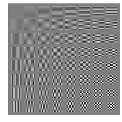
Figure 2.1: Scaled eigenvectors ($\mathbb{U}\mathbb{D}^{1/2}$) of $\mathbb{L}_{(2D)}$ on an $8\times 8$ grid. Random vectors $\mathbb{s}$ which place large weights on ‘high-frequency’ patterns will be penalised.

We can obtain an analytical expression for the eigendomposition ($\mathbb{L}=\mathbb{U}\mathbb{D}\mathbb{U}^{T}$) of this Laplacian as the matrix encodes the recurrence requirements of the Discrete Cosine Transform (DCT). The analytical form of DCT-II is known (Strang (1999), Ahmed et al. (1974)) and therefore (with $j,k$ ranging over $0,...,N-1$):

$$\mathbb{U}_{jk}=\cos\left((j+1/2)k\pi/N\right)$$ (5)

$$\mathbb{\gamma}_{k}=2-2\cos(k\pi/N)$$

This can be integrated into our framework with $\mathbb{h}_{i}(\theta)=\theta_{1}+\theta_{2}\gamma_{i}$ for fixed $\gamma_{i},i=1,\ldots,V$, giving:

$$\mathbb{Q}(\theta)=\theta_{1}\mathbb{I}_{V}+\theta_{2}\mathbb{U}\text{diag}(\{\gamma_{i}\})\mathbb{U}^{T}$$

We can extend this decomposition to 2- and 3- dimensional grids using either (3) or (4) respectively. These observations afford further insight into the random vector $\mathbb{s}\sim\mathcal{N}(\mathbb{0},\mathbb{Q}(\theta)^{-}1)$ as

$$\ln f(\mathbb{s}|\theta)\propto c+\theta_{1}\mathbb{s}^{T}\mathbb{s}+\theta_{2}\sum_{i=1}^{V}\gamma_{i}(\mathbb{U}^{T}\mathbb{s})_{i}^{2}$$

from which we see that the distribution penalises by a flexible amount, $\theta_{2}$, those DCT-II coefficients, $(\mathbb{U}^{T}\mathbb{s})_{i}^{2}$, corresponding to large eigenvalues, $\gamma_{i}$. Those indices $i$ for which the eigenvalues $\gamma_{i}$ is large are exactly those for which the corresponding eigenvectors represent high frequency activity, as illustrated in Fig 2.1.

2.4 Other models

Rue and Held (2005) discuss the link between another graphical model and discrete linear transform. They showed that for circulant block precision matrices the relevant transform is the Discrete Fourier Transform (DFT). The difference between DFT and DCT-II being the relevant boundary conditions where DFT essentially considers graphs on a loop or torus, while DCT-II has free edges. While that work considered graphs on regular grids it did not make fully clear the transform interpretation or the implication in terms of penalisation.

Another popular linear transform that yields an interpretable graphical model is the Discrete Wavelet Transform (DWT). Suppose the IDWT provides the eigenvectors $\mathbb{U}$ of a precision matrix for a particular orthogonal wavelet basis. A simple example would be a model for a fully connected graph. Here the discrete Haar or D4 wavelet bases, combined with the eigenvalue $0$ for the eigenvector $\mathbb{1}$, as usual, and the eigenvalue $n$ for all other eigenvectors produce the required Laplacian matrix, $n\mathbb{I}-\mathbb{1}\mathbb{1}^{T}$.

Table 2.1: collection of latent covariance structures
$\mathbb{U}$	complexity	graphical model
DCT	$\mathcal{O}(n\ln n)$	autocorrelation
DCT $\otimes$ DCT	$\mathcal{O}(n^{\prime}\ln n^{\prime})$, $n^{\prime}=\max(n_{1},n_{2})$	spatial autocorrelation
DFT	$\mathcal{O}(n\ln n)$	circulant autocorrelation
DWT-Haar	$\mathcal{O}(n)$	fully connected groups
DWT $\otimes$ DCT	$\mathcal{O}(\max\{n_{1},$ $n_{2}\log n_{2}\})$	fully connected groups autocorrelated over time
Any	$\mathcal{O}(n^{3})$	aribitrary precision matrix
Any $\otimes$ DCT	$\mathcal{O}(\max\{n_{1}^{3},$ $n_{2}\log n_{2}\})$	aribitrary precision matrix autocorrelated over time

The decompositions in (3) and (4) also help with Laplacians which are the product of characteristically different graphs. For instance suppose we were interested in modelling daily fluctuations of temperature at different spatial locations. Midnight being both the end and start of a day, $\mathbb{L}_{1}$ could represent a model where the daily timeseries was associated at its edges with a DFT based decomposition. While spatial dependency between nearby locations could be expressed with a 2D DCT based graph $\mathbb{L}_{2}\oplus\mathbb{L}_{3}$. These models are summarised in Table 2.1.

A further set of rules for generating new covariance structures involves powers and sums of known structures.

$$\mathbb{Q}^{\prime}(\theta)=\mathbb{Q}(\theta)^{n}+\mathbb{Q}(\theta)^{m}=\mathbb{U}(\mathbb{D}(\theta)^{n}+\mathbb{D}(\theta)^{m})\mathbb{U}^{T}$$

So that $\mathbb{h}^{\prime}_{i}(\theta)=\mathbb{h}_{i}(\theta)^{n}+\mathbb{h}_{i}(\theta)^{m}$. For example, with the DCT based neighbourhood model and $n=2,m=0$, we find $\mathbb{Q}^{2}$ expresses second order relationships among the nodes. Similarly we can mix parameters:

$$\mathbb{Q}^{\prime}(\theta^{\prime})=\mathbb{Q}(\theta_{(1)})+\mathbb{Q}(\theta_{(2)})=\mathbb{U}(\mathbb{D}(\theta_{(1)})+\mathbb{D}(\theta_{(2)}))\mathbb{U}^{T}$$

So that $\mathbb{h}^{\prime}_{i}(\theta)=\mathbb{h}^{\prime}_{i}(\theta_{(1)})+\mathbb{h}^{\prime}_{i}(\theta_{(2)})$. These combinatorial rules for kronecker structure, powers, sums, and combination of spectral curves provide a powerful framework for working tractably with a range of nondiagonal latent covariance structures.

3 Model

In this section we propose an extension, infinite Sparse Structured Factor Analysis (iSSFA), to the work of Knowles and Ghahramani (2007). Our model provides nondiagonal covariance structure for the latent features. The full specification of our model is:

$\mathbb{Z}\sim IBP(\alpha,\beta)$	feature activations
$\mathbb{A}_{t,j}\sim\mathcal{N}(\tau_{j},\nu_{j}^{-1})\ \ j=1,...$	feature weights
$\mathbb{S}_{j,:}^{T}\sim\mathcal{N}(\mathbb{0},\mathbb{Q}(\theta)^{-1})\ \ \ j=1,...$	features
$\mathbb{E}_{t,:}\sim\mathcal{N}(\mathbb{0},\sigma^{2}\mathbb{I})\ \ \ \ t=1,...,T$	measurement error
$\sigma^{2}\sim\mathcal{IG}(a,b)$	noise level
$\alpha\sim\mathcal{G}(e_{\alpha},f_{\alpha})$	IBP strength
$\beta\sim\mathcal{G}(e_{\beta},f_{\beta})$	IBP repulsion
$\nu_{j}\sim\mathcal{G}(e_{\nu},f_{\nu})$	weights’ precisions
$\tau_{j}\sim\mathcal{N}(m_{\tau},r_{\tau}^{-1})$	weights’ means
$\ln\theta_{p}\sim\mathcal{N}(m_{p},r_{p}^{-1}),\ \ p=1,\ldots,P$	feature parameters

Where we model $\mathbb{Q}(\theta)=g(\theta)\mathbb{I}_{V}+h(\theta)\mathbb{L}=\theta_{1}\mathbb{I}_{V}+\theta_{2}\mathbb{L}$. We will take $\mathbb{L}$ to be a multi-dimensional neighbourhood graph as discussed in Section 2.3 and hence made efficient through the DCT. In our simulated example of Section 5 this will be a 2D graph, while in neuroimaging example of Section 6 it will be 3D. However, the scheme provided below would work for other suitable $\mathbb{Q}$ as described in Section 2 with little modification. Observe that the distribution of features requires that they be smooth to a level determined by the spatial hyperparameter $\theta$, which we then learn from the data.

Compared to Knowles and Ghahramani (2007) the enriched prior on $\mathbb{A}$ allows different means and variances for each column. This adds expressivity to the model when sources are not identically distributed. Also, we observe that zero mean weights in $\mathbb{A}$ can lead more easily to degenerate situations with respect to sparsity in which $\mathbb{Z}=\mathbb{1}_{T,K}$. We will see in Section 4.2 that non-zero means enable the relevant spatial vector $\mathbb{S}_{k,:}^{T}$ to explain residuals when deciding whether to activate a feature for an observation $\mathbb{Z}_{t,k}$.

4 Gibbs sampler

Building on the methods of Knowles and Ghahramani (2007) we can construct a Gibbs sampler for the model proposed in Section 3. The sampler is approximate in that we use a Laplace approximation to the posterior distribution of the latent feature parameters.

For clarity, in our notation $\mathbb{M}_{i,:}$ means the $i^{th}$ row of a matrix, or, if $i$ is a set, all rows indexed by elements of the set. A minus sign in the index $\mathbb{M}_{-i,:}$ means all rows except the $i^{th}$, with a similar convention for sets. Similar conventions apply to indexing of columns.

4.1 Conditional distributions of latent features, $\mathbb{S}_{k,:}^{T}$

Consider resampling the feature $\mathbb{S}_{k,:}$. Define a residual:

$$\boldsymbol{\epsilon}_{t}^{k}=(\mathbb{Y}_{t,:}-(\mathbb{A}_{t,-k}\circ\mathbb{Z}_{t,-k})\mathbb{S}_{-k,:})^{T}$$

The Gibbs conditional distribution for $\mathbb{S}_{k,:}^{T}$ is, then, multivariate normal

$$\mathbb{S}_{k,:}^{T}|\mathbb{A},\mathbb{Z},\mathbb{S}_{-k,:},\sigma^{2},\mathbb{Y}\sim\mathcal{N}(\boldsymbol{\mu}_{\mathbb{S}},\boldsymbol{\Sigma}_{\mathbb{S}})$$

with

$$\boldsymbol{\mu}_{\mathbb{S}}=\left(\frac{\sum_{t=1}^{T}\mathbb{A}_{t,k}^{2}\mathbb{Z}_{t,k}}{\sigma^{2}}\mathbb{I}+\mathbb{Q}\right)^{-1}\left(\frac{1}{\sigma^{2}}\sum_{t=1}^{T}\mathbb{A}_{t,k}\mathbb{Z}_{t,k}\boldsymbol{\epsilon}_{t}^{k}\right)$$

$$\boldsymbol{\Sigma}_{\mathbb{S}}=\left(\frac{\sum_{t=1}^{T}\mathbb{A}_{t,k}^{2}\mathbb{Z}_{t,k}}{\sigma^{2}}\mathbb{I}+\mathbb{Q}\right)^{-1}$$

The feature vectors function as a basis for the latent data space. We can see from these conditional distributions that the Gibbs sampler bears a resemblance to the Gram-Schmidt orthogonalisation procedure. Each feature is treated as though it were the final vector in the procedure, the effects of the other features having being subtracted from the data to leave a residual vector which is then normalised by application of a covariance matrix.

4.2 Activation of shared features within $\mathbb{Z}_{t,k}$

Sampling of $\mathbb{Z}$ occurs in two phases. We describe features as shared when $m_{k}=\sum_{t=1}^{T}\mathbb{Z}_{t,k}>1$ and as unique when $m_{k}=1$. A draw from the two parameter IBP is obtained by, for the $t^{th}$ observation, activating each shared feature with probability $\sum_{r=1}^{t-1}\mathbb{Z}_{r,k}/(\beta+t-1)$ and then drawing a set of $\text{Poisson}(\alpha\beta/(\beta+t-1))$ unique features (Knowles and Ghahramani (2007)). The rows of the matrix are exchangeable so that conditional on the other observations, the $t^{th}$ observation may be treated as the $T^{th}$. When doing posterior inference, this structure leads naturally to two stages, in which we sample shared features as Bernoulli, and a number of unique features as Poisson. The following step deals with resampling of shared features.

For $\mathbb{Z}$ we will approach sampling entry-wise, using the technique of Knowles and Ghahramani (2007) in defining a ratio of conditionals $r=r_{l}r_{p}$. Where $r_{p}$ is available from section 2.1 of that work, $r_{p}=\frac{m_{k,-t}}{\beta+T-1-m_{k,-t}}$, with $m_{k,-t}$ being the number of times the $k^{th}$ factor has been activated, excluding observation $t$. In our case $r_{l}$ is different with:

$$r_{l}=\frac{p(\mathbb{Y}_{t,:}|\mathbb{A}_{:,-k},\mathbb{A}_{-t,k},\mathbb{S},\mathbb{Z}_{:,-k},\mathbb{Z}_{-t,k},\mathbb{Z}_{t,k}=1,\sigma^{2})}{p(\mathbb{Y}_{t,:}|\mathbb{A}_{:,-k},\mathbb{A}_{-t,k},\mathbb{S},\mathbb{Z}_{:,-k},\mathbb{Z}_{-t,k},\mathbb{Z}_{t,k}=0,\sigma^{2})}$$

The required marginal distribution of the numerator is again Gaussian:

$$\mathbb{Y}_{t,:}^{T}|\mathbb{A}_{:,-k},\mathbb{A}_{-t,k},\mathbb{S},\mathbb{Z}_{:,-k},\mathbb{Z}_{-t,k},\mathbb{Z}_{t,k}=1,\sigma^{2},\cdot\sim$$

$$\mathcal{N}\left(\left[(\mathbb{A}_{t,-k}\circ\mathbb{Z}_{t,-k})\mathbb{S}_{-k,:}\right]^{T}+\mathbb{S}_{k,:}^{T}\tau_{k},\ \ \sigma^{2}\mathbb{I}_{V}+\frac{1}{\nu_{k}}\mathbb{S}_{k,:}^{T}\mathbb{S}_{k,:}\right)$$

This presents an important modelling difference from the work in Knowles and Ghahramani (2007) where, due to the assumption of zero-mean feature weights ($\tau_{k}=0$), the mean of the numerator distribution would not feature $\mathbb{S}_{k,:}^{T}$. That fact would force the algorithm to explain the residual $(\mathbb{Y}_{t,:}-(\mathbb{A}_{t,-k}\circ\mathbb{Z}_{t,-k})\mathbb{S}_{-k,:})^{T}$ using only the covariance structure. Non-zero means $\tau_{k}$ allows a feature vector to help explain the residual when sampling a feature activation $\mathbb{Z}_{t,k}$. Now set:

$$\mathbb{r}_{0}=\mathbb{Y}_{t,:}^{T}-\left[(\mathbb{A}_{t,-k}\circ\mathbb{Z}_{t,-k})\mathbb{S}_{-k,:}\right]^{T}$$

$$\mathbb{r}_{1}=\mathbb{Y}_{t,:}^{T}-\left[(\mathbb{A}_{t,-k}\circ\mathbb{Z}_{t,-k})\mathbb{S}_{-k,:}\right]^{T}-\mathbb{S}_{k,:}^{T}\tau_{k}$$

We can now evaluate $\ln r_{l}$ as:

$$\ln r_{l}=\ln p(\mathbb{Y}_{t,:}|\mathbb{Z}_{t,k}=1,\cdot)-\ln p(\mathbb{Y}_{t,:}|\mathbb{Z}_{t,k}=0,\cdot)=$$

$$\ \ \ -\frac{1}{2}\ln\left(1+\frac{1}{\sigma^{2}\nu_{k}}\mathbb{S}_{k,:}\mathbb{S}_{k,:}^{T}\right)-\frac{1}{2\sigma^{2}}\mathbb{r}_{1}^{T}\mathbb{r}_{1}$$

$$\ \ \ +\frac{1}{2}((\sigma^{2}\nu_{k})(\sigma^{2}+\mathbb{S}_{k,:}\mathbb{S}_{k,:}^{T}/\nu_{k}))^{-1}(\mathbb{S}_{k,:}\mathbb{r}_{1})^{2}$$

$$\ \ \ +\frac{1}{2\sigma^{2}}\mathbb{r}_{0}^{T}\mathbb{r}_{0}$$

Hence, despite both the precision and covariance matrices for the numerator being dense, the density may be evaluated in $\mathcal{O}(V)$ time and memory as the main calculations are dot products of dense vectors in $\mathbb{R}^{V}$. For the shared features, $k$, we can now sample $\mathbb{Z}_{t,k}\sim\text{Bern}\left(\frac{r_{l}r_{p}}{r_{l}r_{p}+1}\right)=\text{Bern}((1+\exp(-\ln(r_{l}r_{p})))^{-1})$.

We use the techniques described in Pearce and White (2016) to efficiently parallelise these calculations across a compute cluster.

4.3 Feature weights for shared features, $\mathbb{A}_{t,k}$

Setting $\mu_{t}=[(\mathbb{A}_{t,-k}\circ\mathbb{Z}_{t,-k})\mathbb{S}_{-k,:}]^{T}$, the Gibbs conditional for $\mathbb{A}_{t,k}$ is Gaussian with:

$$\mathbb{A}_{t,k}|\cdot\sim\mathcal{N}(\mu_{A},\zeta_{A})$$

with

$$\mu_{A}=\left(\nu_{k}+\frac{\mathbb{S}_{k,:}\mathbb{S}_{k,:}^{T}}{\sigma^{2}}\right)^{-1}\left(\frac{1}{\sigma^{2}}\mathbb{S}_{k,:}(\mathbb{Y}_{t,:}^{T}-\mu_{t})+\nu_{k}\tau_{k}\right)$$

$$\zeta_{A}=\left(\nu_{k}+\frac{\mathbb{S}_{k,:}\mathbb{S}_{k,:}^{T}}{\sigma^{2}}\right)^{-1}$$

4.4 Activating unique features

In order to complete a draw from the Indian Buffet Process we must sample unique features for each observation, a task we will tackle by a Metropolis-Hastings step for each observation. The IBP is exchangeable (Griffiths and Ghahramani (2011), Knowles and Ghahramani (2007)) hence the $t^{th}$ observation may be treated as the $T^{th}$. Define $J_{t}$ to be the set of indices of $n$ new components for observation $t$. We set the number of such components and the parameters and weights associated with them as $\omega$ = $(n,\{\tau_{j}\},\{\nu_{j}\},\{a_{j}\})$ where the $a_{j}$ are weights for features.

We make a proposal $\omega^{*}$ in three steps: sampling the number of new sources $n$, then their parameters $\{\tau_{j}\},\{\nu_{j}\}|n$ and finally the weightings $a_{j}|\{\tau_{j}\},\{\nu_{j}\}$. Note that at this point the feature vectors will be marginalised out. We then choose to accept or reject the proposal via an MH step. It will be convenient to write,

$$\boldsymbol{\mu}=\mathbb{S}_{-J_{t},:}^{T}(\mathbb{A}_{t,-J_{t}}\circ\mathbb{Z}_{t,-J_{t}})^{T}$$

as the values of the columns of $\mathbb{A},\mathbb{Z}$, and rows of $\mathbb{S}$ corresponding to shared features enter in to our calculations only through the mean of $\mathbb{Y}_{t}$. Afterwards, conditional on MH acceptance, we will sample the new sources $\{\mathbb{s}_{j}\}_{j\in J_{t}}$ (see Section 4.5). That is to say we block sample $p(\omega,\{\mathbb{s}_{j}\}|\cdot)$ as $p(\{\mathbb{s}_{j}\}|\omega,\cdot)p(\omega|\cdot)$ for each $t$.

To begin, we use the respective priors to generate proposals:

$$n\sim Poi\left(\frac{\beta\alpha}{\beta+T-1}\right)$$

$$\tau_{j}|n\sim\mathcal{N}(m_{\nu},r_{\nu}^{-1})\ ,\ \ j\in J_{t}$$

$$\nu_{j}|n\sim\mathcal{G}(e_{\nu},f_{\nu})\ ,\ \ j\in J_{t}$$

$$a_{j}|n,\tau_{j},\nu_{j}\sim\mathcal{N}(\tau_{j},\nu_{j}^{-1})\ ,\ \ j\in J_{t}$$

Then form an acceptance probability ratio where we make use of the proposal $q(\omega^{*}|\omega)$ being equal to the prior $g(\omega^{*})$ so that:

$$\psi=\frac{p(\omega^{*}|\mathbb{Y}_{t,:}^{T},\cdot)q(\omega|\omega^{*})}{p(\omega|\mathbb{Y}_{t,:}^{T},\cdot)q(\omega^{*}|\omega)}=\frac{p(\mathbb{Y}_{t,:}^{T}|\omega^{*},\cdot)}{p(\mathbb{Y}_{t,:}^{T}|\omega,\cdot)}$$

Which forms the basis of the acceptance probability.

We now focus on the density for $f(\mathbb{Y}_{t,:}^{T}|\omega)$, for which we need to marginalise out the features corresponding to the weights we sampled. In their prior, the features $\{\mathbb{s}_{j}\}$ are, conditional on the hyperparameters, IID multivariate normal. Let us stack them into a single vector, and define a block matrix which we will use to manipulate them.

$$\mathbb{r}=\left[\begin{matrix}\mathbb{s}_{1}\\ \mathbb{s}_{2}\\ \vdots\\ \mathbb{s}_{n}\end{matrix}\right]\ \ ,\ \mathbb{C}=\left[a_{1}\mathbb{I}_{V},a_{2}\mathbb{I}_{V},\cdots,a_{n}\mathbb{I}_{V}\right]$$

So that $\mathbb{r}$ is $(nV\times 1)$ and $\mathbb{C}$ is $(V\times nV)$. The conditional distribution of the observations is, then:

$$\mathbb{Y}_{t,:}^{T}|\{a_{j}\},\mathbb{r},\cdot\sim\mathcal{N}_{V}\left(\boldsymbol{\mu}+\mathbb{C}\mathbb{r},\sigma^{2}\mathbb{I}_{V}\right)$$

$$\mathbb{r}\sim\mathcal{N}_{nV}(\mathbb{0},\mathbb{I}_{n}\otimes\mathbb{Q}^{-1})$$ (6)

Hence, using results on the multivariate normal distribution:

$$\mathbb{Y}_{t,:}^{T}|\{a_{j}\},\cdot\sim\mathcal{N}_{V}\left(\boldsymbol{\mu},\ \ \sigma^{2}\mathbb{I}+\left(\sum_{j\in J_{t}}a_{j}^{2}\right)\mathbb{Q}^{-1}\right)$$

This density function provides the numerator and denominator of $\psi$, enabling us to calculate the acceptance probability for the proposal.

4.5 Drawing spatial feature vectors for unique features

This section continues with the notation used in Section 4.4, as we are completing a block draw. For each observation $t$ we need to draw the spatial features from the distribution $\{\mathbb{s}_{j}\}|\omega,\cdot$. Hence, reversing the conditioning in (4.4) we see that the posterior for $\mathbb{r}$ is again Gaussian:

$$\mathbb{r}|\mathbb{Y}_{t,:}^{T},\cdot\sim\mathcal{N}(\boldsymbol{\mu}_{\mathbb{r}},\boldsymbol{\Sigma}_{\mathbb{r}})$$

$$\boldsymbol{\mu}_{\mathbb{r}}=\left(\frac{1}{\sigma^{2}}\mathbb{C}^{T}\mathbb{C}+\mathbb{I}_{n}\otimes\mathbb{Q}\right)^{-1}\left(\frac{1}{\sigma^{2}}\mathbb{C}^{T}(\mathbb{Y}_{t,:}^{T}-\boldsymbol{\mu})\right)$$

$$\boldsymbol{\Sigma}_{\mathbb{r}}=\left(\frac{1}{\sigma^{2}}\mathbb{C}^{T}\mathbb{C}+\mathbb{I}_{n}\otimes\mathbb{Q}\right)^{-1}$$

4.6 Sampling the noise level $\sigma^{2}$

If we place an inverse gamma prior on $\sigma^{2}\sim\mathcal{IG}(u,v)$ then conditional on the other variables, the result is conjugate. Write $\boldsymbol{\epsilon}_{t}=\mathbb{Y}_{t,:}-(\mathbb{A}_{t,:}\circ\mathbb{Z}_{t,:})\mathbb{S}$ and note that there are $T$ such rows. The conditional follows an inverse gamma distribution:

$$\sigma^{2}|\mathbb{Y},\cdot\sim\mathcal{I}G\left(\frac{TV}{2}+u,v+\frac{1}{2}\sum_{t=1}^{T}\sum_{v=1}^{V}\boldsymbol{\epsilon}_{t,v}^{2}\right)$$

4.7 Sampling spatial parameters $\theta$

As the paramaters of the latent feature must be non-negative we place our prior on their logarithms $\xi_{p}=\ln\theta_{p}$ for $p=1,\ldots,P$. We sample from the conditional posterior for $\xi$ using a Laplace approximation (Rue et al. (2009)) to the posterior distribution, that is to:

$$p(\xi|\mathbb{S},\cdot)\propto p(\mathbb{S}|\xi,\cdot)f(\xi)$$

We find that this approach works well across scales of $\theta$ without the need for additional MCMC tuning parameters required by asymptotically exact methods. For the prior we will assume independent normal distributions for the $\xi_{p}$ so that $f(\xi)=\prod_{p=1}^{P}\mathcal{N}(\xi_{2};m_{\xi_{2}},r_{\xi_{2}})$.

To perform the Laplace approximation we must find the MAP estimate of the parameters. In our example model $\mathbb{h}_{i}(\theta)=\theta_{1}+\theta_{2}\gamma_{i}$ so that $\mathbb{Q}=\theta_{1}\mathbb{I}_{V}+\theta_{2}\mathbb{L}$. The log posterior is:

$$\ln f(\xi|\mathbb{S},\cdot)=\ln f(\xi|\mathbb{S})=c+\frac{K}{2}\sum_{i=1}^{V}\ln(\theta_{1}+\theta_{2}\gamma_{i})$$

$$\ \ \ -\frac{1}{2}\sum_{i=1}^{K}\mathbb{S}_{i,:}(\theta_{1}\mathbb{I}+\theta_{2}\mathbb{L})\mathbb{S}_{i,:}^{T}$$

$$\ \ \ -\frac{r_{\xi_{1}}}{2}\xi_{1}^{2}+m_{\xi_{1}}r_{\xi_{1}}\xi_{1}-\frac{r_{\xi_{2}}}{2}\xi_{2}^{2}+m_{\xi_{2}}r_{\xi_{2}}\xi_{2}-\xi_{1}-\xi_{2}$$

Which, after applying the chain rule, provides the following first derivatives:

$$\frac{\partial\ln p(\xi|\mathbb{S})}{\partial\xi_{1}}=\theta_{1}\left(\frac{K}{2}\sum_{i=1}^{V}\frac{1}{\theta_{1}+\theta_{2}\gamma_{i}}-\frac{1}{2}\sum_{i=1}^{K}\mathbb{S}_{i,:}\mathbb{S}_{i,:}^{T}\right)$$

$$\ \ \ -r_{\xi_{1}}\xi_{1}+m_{\xi_{1}}r_{\xi_{1}}-1$$

$$\frac{\partial\ln f(\xi|\mathbb{S})}{\partial\xi_{2}}=\frac{K}{2}\sum_{i=1}^{V}\frac{\gamma_{i}}{\theta_{1}+\theta_{2}\gamma_{i}}-\frac{1}{2}\sum_{i=1}^{K}\mathbb{S}_{i,:}\mathbb{L}\mathbb{S}_{i,:}^{T}$$

$$\ \ \ -r_{\xi_{2}}\xi_{2}+m_{\xi_{2}}r_{\xi_{2}}-1$$

After which the second derivatives required to populate the negative of the Hessian matrix, $\mathbb{H}$, can also be found:

$$\frac{\partial^{2}\ln p(\xi|\mathbb{S})}{\partial\xi_{1}^{2}}=\frac{\partial\ln p(\xi|\mathbb{S})}{\partial\xi_{1}}-\theta_{1}^{2}\frac{K}{2}\sum_{i=1}^{V}(\theta_{1}+\theta_{2}\gamma_{i})^{-2}-r_{\xi_{1}}$$

$$\frac{\partial^{2}\ln p(\xi|\mathbb{S})}{\partial\xi_{2}^{2}}=\frac{\partial\ln p(\xi|\mathbb{S})}{\partial\xi_{2}}-\theta_{2}^{2}\frac{K}{2}\sum_{i=1}^{V}\left(\frac{\gamma_{i}}{\theta_{1}+\theta_{2}\gamma_{i}}\right)^{2}-r_{\xi_{2}}$$

$$\frac{\partial^{2}\ln p(\xi|\mathbb{S})}{\partial\xi_{1}\xi_{2}}=-\theta_{1}\theta_{2}\frac{K}{2}\sum_{i=1}^{V}\frac{\gamma_{i}}{\left(\theta_{1}+\theta_{2}\gamma_{i}\right)^{2}}$$

We then use numerical optimisation to find a MAP estimate $\hat{\xi}$, following which we sample from the approximate conditional posterior distribution:

$$\xi|\mathbb{S},\cdot\sim\mathcal{N}(\hat{\xi},\mathbb{H}^{-1})$$

If required, this distribution can be used as a proposal for a corrected MH accept/reject step:

$$\frac{f(\xi^{\prime}|\mathbb{S},\cdot)N(\xi;\hat{\xi},\mathbb{H}^{-1})}{f(\xi|\mathbb{S},\cdot)N(\xi^{\prime};\hat{\xi},\mathbb{H}^{-1})}$$

Which, if the approximation is good should have a high acceptance rate, and where all the quantities can be evaluated using previous computations. However, in the examples below we sample from the Laplace approximation directly.

4.8 Sampling the IBP strength $\alpha$

We use a rate parameterised alternative to that in Knowles and Ghahramani (2007). Let $H_{T}(\beta)=\sum_{i=1}^{T}\frac{\beta}{i+\beta-1}$, then:

$$P(\alpha|\mathbb{Z},\beta)\propto P\left(\mathbb{Z}|\alpha,\beta\right)P(\alpha)$$

$$\propto\mathcal{G}(\alpha;K_{+}+e_{\alpha},f_{\alpha}+H_{T}(\beta))$$

Where $K_{+}$ is the number of non-zero columns of $\mathbb{Z}$.

4.9 Sampling the IBP repulsion $\beta$

We will sample this via a metropolis step. We use the shape-rate parametrised Gamma prior $\beta\sim\mathcal{G}(e_{\beta},f_{\beta})$. In order to ensure non-negativity we will work with parameter logarithms. We take a Normal distribution for the proposal $q(\psi|\psi^{*})=\mathcal{N}(\psi^{*};\psi,s_{\beta})$. Write $m_{k}=\sum_{t=1}^{T}\mathbb{Z}_{t,k}$. $B(.,.)$ is the beta function, $H_{T}(\beta)$ is as above, and $K_{l}$ is the number of columns whose entries correspond to the integer $l$ expressed in binary (reading a column of $\mathbb{Z}$ downwards yields a binary number $0\leq l\leq 2^{T}-1$). The likelihood ratio is:

$$L=\ln\frac{P(\mathbb{Z}|\alpha,\psi^{*})}{P(\mathbb{Z}|\alpha,\psi)}=-\alpha H_{T}(\beta^{*})+\alpha H_{T}(\beta)$$

$$=\sum_{k=1}^{K_{+}}\left[\ln\Gamma(T-m_{k}+\beta^{*})-\ln\Gamma(T-m_{k}+\beta)\right]$$

$$\ \ \ +K_{+}(\ln\Gamma(T+\beta)-\ln\Gamma(T+\beta^{*}))$$

$$\ \ \ +\alpha(H_{T}(\beta)-H_{T}(\beta^{*}))$$

So that the log Metropolis-Hastings ratio is found as:

$$\ln a_{\beta\rightarrow\beta^{*}}=L+e_{\beta}\ln\beta^{*}-f_{\beta}\beta^{*}-e_{\beta}\ln\beta+f_{\beta}\beta$$

$$=L+e_{\beta}[\ln\beta^{*}-\ln\beta]+f_{\beta}[\beta-\beta^{*}]$$

4.10 Sampling weight precisions $\nu_{k}$

The Gibbs distibution for $\nu_{k}$ is a Gamma:

$$\nu_{k}|\{\mathbb{A}_{:,k}\}_{t:Z_{t,k}=1},\cdot\sim\mathcal{G}(\tilde{e}_{\nu},\tilde{f}_{\nu})$$

with

$$\tilde{e}_{\nu}=e_{\nu}+1/2\sum_{i=1}^{T}\mathbb{Z}_{t,k},$$

$$\tilde{f}_{\nu}=\ f_{\nu}+\frac{1}{2}\sum_{i=1}^{T}((\mathbb{A}_{t,k}-\tau)\mathbb{Z}_{t,k})^{2}$$

4.11 Sampling the weight means $\tau_{k}$

The Gibbs distribution $\tau_{k}|\mathbb{A},\mathbb{Z},\cdot$ is normal with:

$$\tau_{k}|\mathbb{A},\mathbb{Z},\cdot\sim\mathcal{N}(\mu_{\tau},\zeta_{\tau})$$

$$\mu_{\tau}=\left(\nu_{k}\sum_{t=1}^{T}\mathbb{Z}_{t,k}+r\right)^{-1}\left(\nu_{k}\sum_{t:Z_{t,k}=1}\mathbb{A}_{t,k}+rm\right)$$

$$\zeta_{\tau}=\left(\nu_{k}\sum_{t=1}^{T}\mathbb{Z}_{t,k}+r\right)^{-1}$$

5 Simulated Example

We generated $T=3000$ observations on a $100\times 100$ grid ($V=10000$). Each observation was a linear combination of 50 features drawn as $\mathbb{S}_{k,:}^{T}\sim\mathcal{N}(\mathbb{0},\mathbb{Q}(1,100)^{-1})$ and then unit normalised. Activation weights were drawn as $\mathbb{Z}_{t,k}\sim Bern(1/20)$ with $\mathbb{A}_{t,k}\sim\mathcal{N}(1,\gamma_{k})$, $50<\gamma_{k}<100$, $\sigma^{2}\sim\mathcal{N}(0,1)$. Additive noise was drawn IID $\mathbb{E}_{t,k}\sim\mathcal{N}(0,1)$. A further holdout dataset of 500 images was drawn from the same distribution for performance testing. The first 10 observed images from the hold out data set are shown in Figure 1(a) and the corresponding latent images in Figure 1(b).

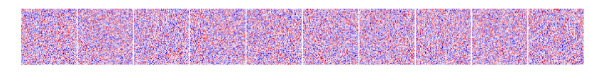
(a) Observed images $\mathbb{Y}_{1:10,:}$ from holdout data

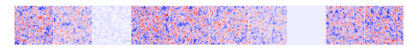
(b) Corresponding latent vectors $(\mathbb{A}\circ\mathbb{Z})_{1:10,:}\mathbb{S}$

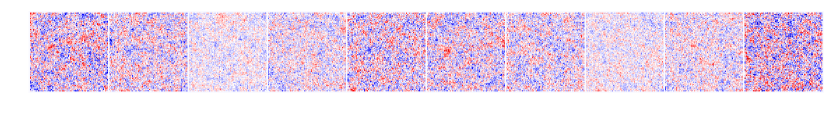
(c) Corresponding PCA reconstruction with $K^{*}=33$

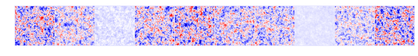
(d) Corresponding Issfa reconstruction $\hat{\mathbb{E}}[(\mathbb{A}\circ\mathbb{Z})_{1:10,:}\mathbb{S}]$

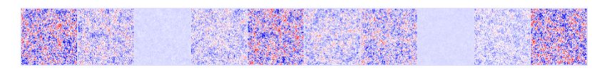
(e) Similar to (d), but using spatially IID prior.

Figure 5.1: Different views of examples from the holdout dataset.

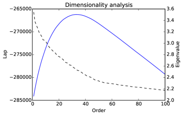
Figure 5.2: Analysis of the dimensionality of the dataset. Blue line shows the Laplace evidence approximation of the dimensionality obtained by Minka’s method (optimising $K^{*}=33$). Black dashed line shows the first 100 eigenvalues of the data covariance matrix.

Six nodes of a high performance compute cluster were used to execute the analysis. Each node had twelve Intel Xeon E5-2620 2.00GHz CPUs and an Nvidia Tesla K20m GPU. The code was written in Julia (Bezanson et al. (2014)) in order to utilise the multiprocessing capabilities of the cluster. Features for the sampler were initialised using a K-means algorithm fit for 15 clusters.

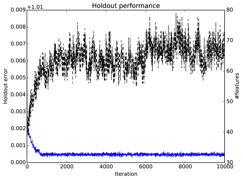
(a) Blue line shows the reconstruction error of the $n^{th}$ MCMC sample on held out data. Black line shows the number of features available.

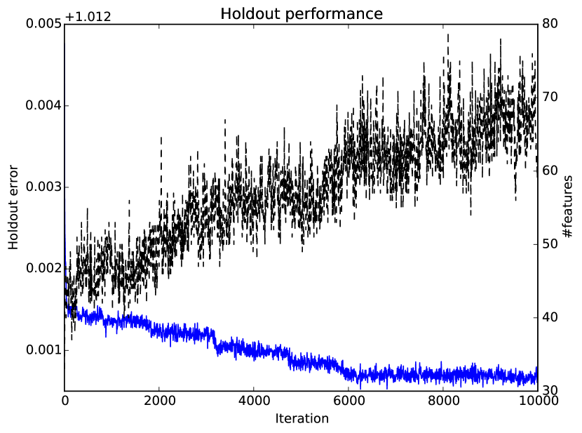
(b) Same as (a), but using spatially IID prior of Knowles and Ghahramani (2007).

Figure 5.3: MCMC sampling traces for analysis of the same dataset under different priors.

Call the true latent data $\mathbb{X}=(\mathbb{A}\circ\mathbb{Z})\mathbb{S}$. Figure 1(d) shows the mean reconstruction of the latent data. That is the Monte Carlo approximation:

$$\mathbb{E}[(\mathbb{A}\circ\mathbb{Z})\mathbb{S}]\approx\hat{\mathbb{X}}^{iSSFA}=\frac{1}{N}\sum_{n=1}^{N}(\mathbb{A}^{(n)}\circ\mathbb{Z}^{(n)})\mathbb{S}^{(n)}$$

where superscripts $(n)$ indicate samples from particular MCMC iterations. Figure 1(e) shows the same estimate under the spatially IID prior of Knowles and Ghahramani (2007). In both cases we used a thinned subsequence of the MCMC samples to obtain the estimate.

(a) Qualitative comparison of feature recovery. Top row: first ten true features. Second row: matched iSSFA features (final MCMC sample); third row matched FastICA features; bottom row: matched eigenvectors. The eigenvectors and the related ICA features appear to vary on a dissimilar scale to the true features. The iSSFA features are all of a similar scale to the true features.

(b) Top ten matched features under the spatially IID prior of Knowles and Ghahramani (2007) (final MCMC sample). Colour normalisation different to (a).

Figure 5.4: Comparison of matched features. Matching done by cosine similarity after normalisation.

We can compare the reconstruction performance of iSSFA model to the reconstruction of the data obtained from PCA / SVD. We estimate the model order using Minka’s method resulting in a setting of $K^{*}=33$. Analysis of dataset dimensionality is shown in Figure 5.2. It is of note that Minka’s method still provides empirically better PCA performance than using the true $K=50$.

We find that, on the holdout data, the reconstruction error using the first $K^{*}=33$ principal eigenvectors is nearly 1.67 times greater than the MCMC reconstruction error $\sum_{t,k}(\mathbb{X}_{t,k}-\hat{\mathbb{X}}^{iSSFA}_{t,k})^{2}$. For the PCA is the solution is a matrix factorisation $\mathbb{X}^{EIG}=\mathbb{W}^{EIG}\mathbb{S}^{EIG}$, where the rows of $\mathbb{S}^{EIG}$ are the first fifty eigenvectors and the corresponding PCs.

We also compare the iSSFA results to another standard matrix decomposition method ICA, implemented through the FastICA algorithm (Hyvärinen and Oja (2000)). This methodology builds on the PCA solution by further factorising the sources $\mathbb{W}^{EIG}=\mathbb{W}^{ICA}\mathbb{U}^{ICA}$. Substituting this into the PCA decomposition of the data $\mathbb{Y}=\mathbb{W}^{ICA}\mathbb{U}^{ICA}\mathbb{S}^{EIG}=\mathbb{W}^{ICA}\mathbb{S}^{ICA}$ (note that we have changed notation from Hyvärinen and Oja (2000)). A comparison of these different sets of features with the true features is shown in Figure 5.4 where it is visible that our nonparametric method finds features that are more similar to the true features.

FastICA attempts to decompose a signal into independent components by maximising the non-Gaussianity of inferred sources $\hat{\mathbb{W}}$, using a metric based on an approximation to negentropy. As can be seen in Fig 5.5 iSSFA produces more highly non-Gaussian estimates of the source distribution than does the FastICA algorithm applied to the same dataset. This is due to the sparsity induced by the Indian Buffet Process, which turns the iSSFA source distribution into a spike-and-slab model. Using sample excess kurtosis as a measure of non-Gaussianity (higher is more super-Gaussian), in the last MCMC iteration iSSFA scored 73.8 while the corresponding FastICA score was 1.1. The shapes of the histograms indicate that this ranking would hold under other reasonable metrics.

Another metric for the quality of the blind source separation is defined in Knowles and Ghahramani (2011), essentially $E_{r}(A,B)=\sum_{k=1}^{K^{TRUE}}\min_{j}\|A_{:,k}-B_{:,j}\|^{2}$. Here we found the ratio of errors to be $E_{r}(\mathbb{S},\mathbb{S}^{ICA})$ $/E_{r}(\mathbb{S},\mathbb{S}^{ISSFA})=1.41$. Whereas under the spatially IID nonparametric prior the same ratio was 0.87, i.e. worse than FastICA. This suggests that, where appropriate, modelling spatial continuity will help to provide a more accurate blind source separation; and also that the number of extra features in the iSSFA model is unlikely to be a sufficient explanation for its better score than ICA.

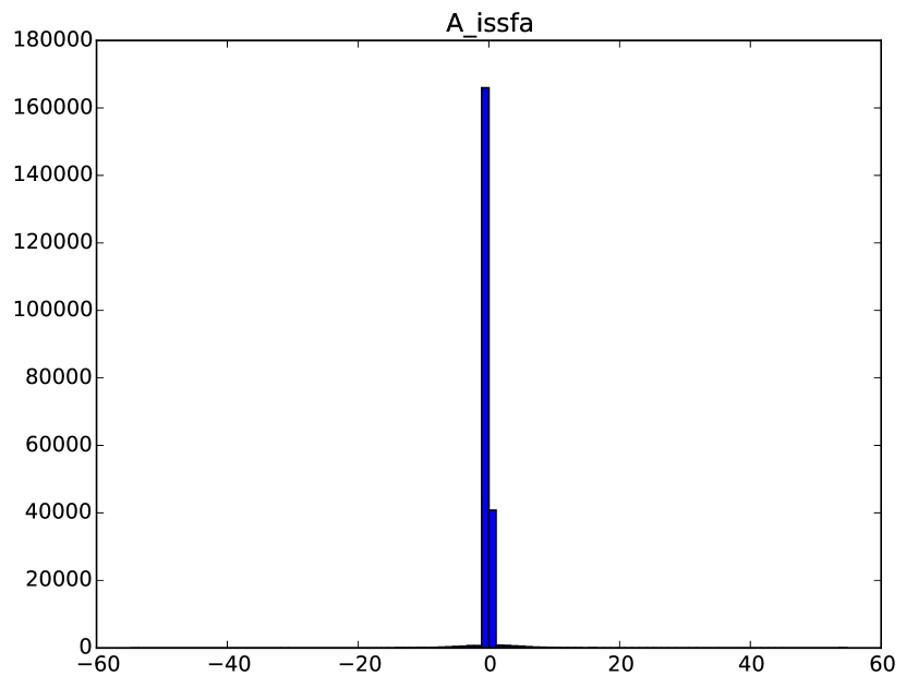
(a) Histogram of sources $\mathbb{W}^{iSSFA}=\hat{(\mathbb{A}\circ\mathbb{Z})}^{iSSFA}$ in the final MCMC iteration, excluding (two) unique features ($\sum_{t}\mathbb{Z}_{t,k}=1$). Sample excess kurtosis: 73.8. The distribution is highly non-Gaussian owing to the spike-and-slab type model. Here the slab is extremely thin due to the level of sparsity.

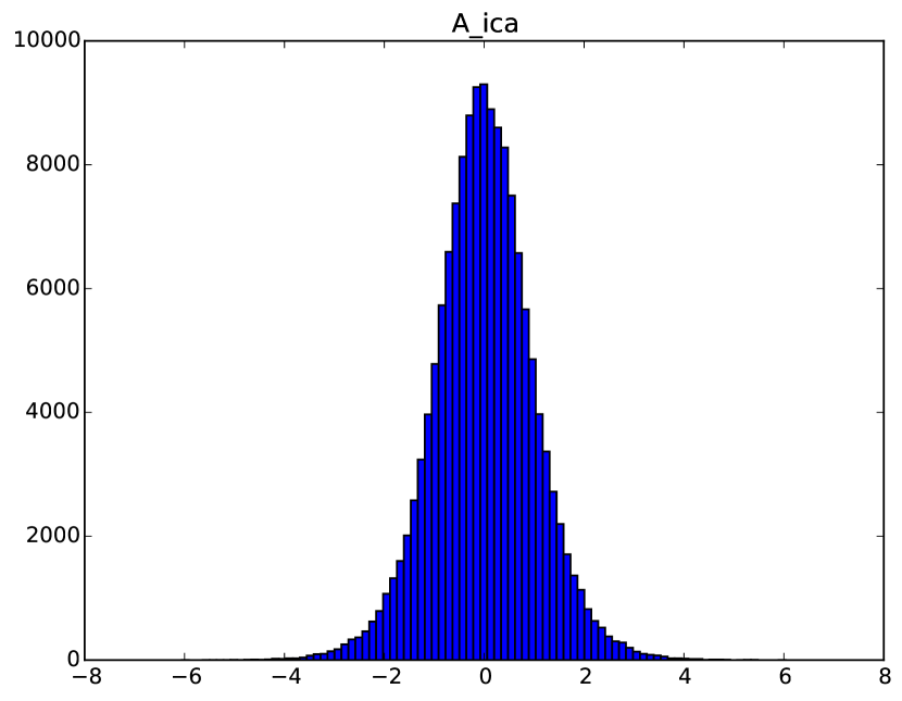
(b) Histogram of sources $\mathbb{W}^{ICA}$ from FastICA. Sample excess kurtosis: 1.1

Figure 5.5: Distribution of inferred sources under iSSFA and FastICA. If one were interested in maximising the non-Gaussianity of inferred sources the sparsity of the iSSFA model produces a more optimal fit by the kurtosis criterion than does the FastICA methodology.

Figure 4(a) shows four rows of features. The top row visualises the first true ten latent features. The following three rows show other types of features matched by cosine similarity: iSSFA features from the final MCMC iteration; FastICA features; and finally PCA features. Figure 5.4 shows matched features obtained under the isFA prior of Knowles and Ghahramani (2007). We can see that modelling latent covariance structure has allowed the model to find a solution which more closely matches the ground truth than FastICA, which produces noisy features that vary on the wrong spatial scale. We also see that even within nonparametric models, accounting for latent covariance has improved feature recovery relative to the IID prior.

Hence, at least when considering sparsely activated data, nonparametric sparse factor analysis can provide a more accurate reconstruction of the original data than can the eigendecomposition. Furthermore relaxation of orthogonality constraints can lead to features which are, individually, more similar to latent features.

6 Neuroimaging application

In this example we consider application of the model to fMRI neuroimaging data, demonstrating the abiity to produce sensible results at scale. The dataset contains 30 subjects from the Cambridge Centre for Ageing and Neuroscience study (Campbell et al. (2015); Shafto et al. (2014)). Subjects watched an editted 8 minute video of a Hitchcock drama Bang! You’re Dead. For each subject this yielded 193 images for a total of $T=193\times 30=5790$, which after preprocessing had a spatial resolution of $V=61\times 73\times 61=271633$.

For fMRI data, naive modelling of spatial dependencies using dense matrices would be infeasible due to the need for inversion and determinants of $V\times V$ covariance matrices. Hence efficient computation is necessary if we wish to model spatial structure. Spatial modelling is well motivated by the fact that the spatial resolution of fMRI is finer than typical parcellations of the brain into functional regions, and hence we should expect neighbouring voxels to often share similar values. Furthermore, as this type of task involves viewing ‘naturalistic’ video, as opposed to an experimental block design, analysis methods must be relatively unconstrained in terms of the form of the time courses and brain regions involved. Hence the model presented is well suited to the requirements of the analysis task.

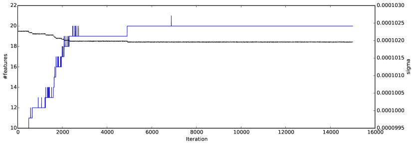
Figure 6.1: Trace plot of the number of features and noise level over MCMC iterations.

We ran the sampler using 6 compute nodes with for 15000 iterations. We used a prior distribution on the noise level which places a soft constraint on the desired reconstruction accuracy. Trace plots of the number of features and inferred noise level are shown in Fig 6.1, where the chain appears to converge.

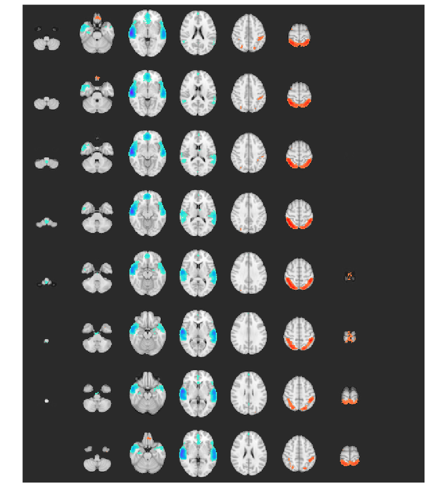
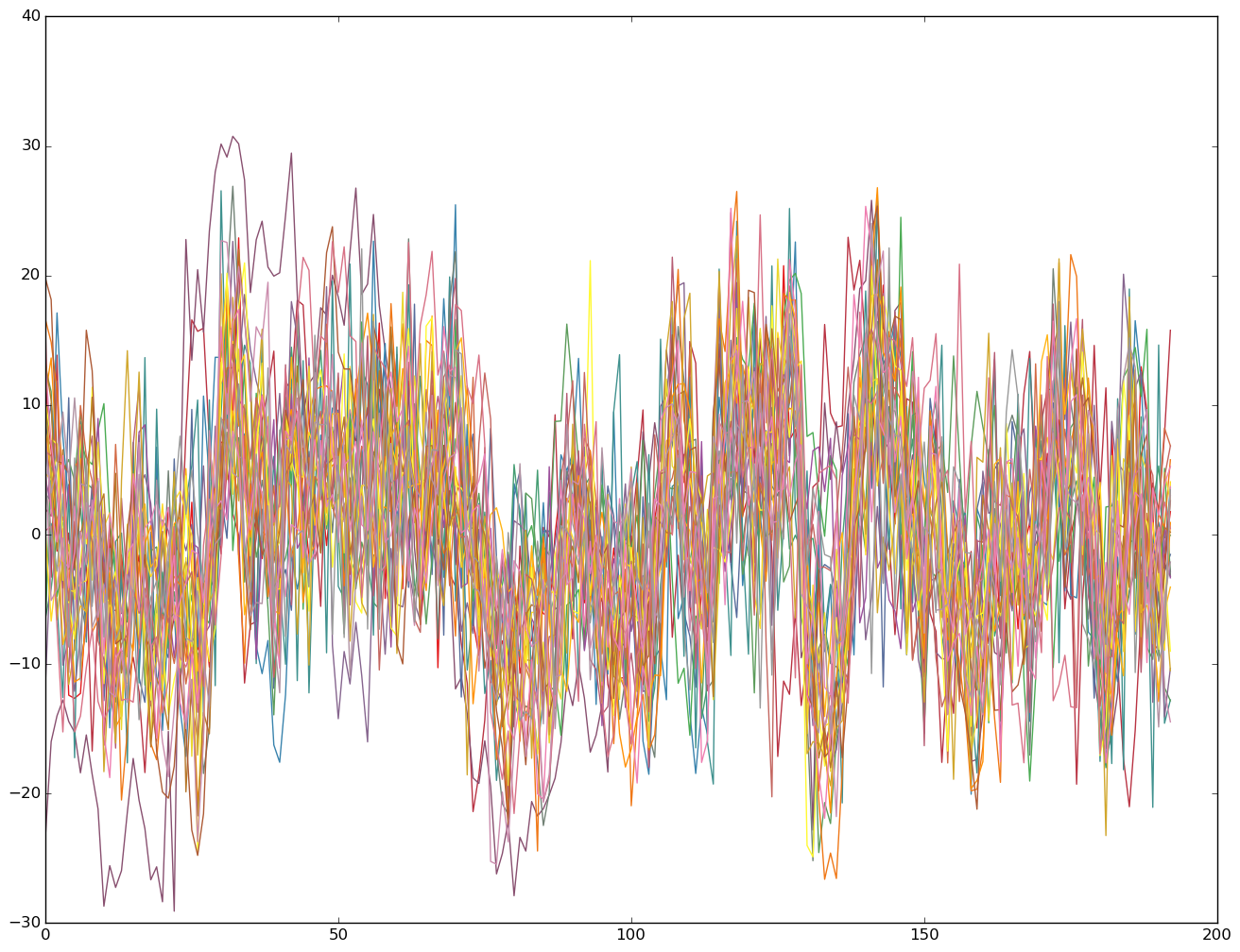
Figure 6.2: The component with highest inter-subject weight correlation. Heavy loadings are on the auditory region, and with opposite sign on the parietal lobe.

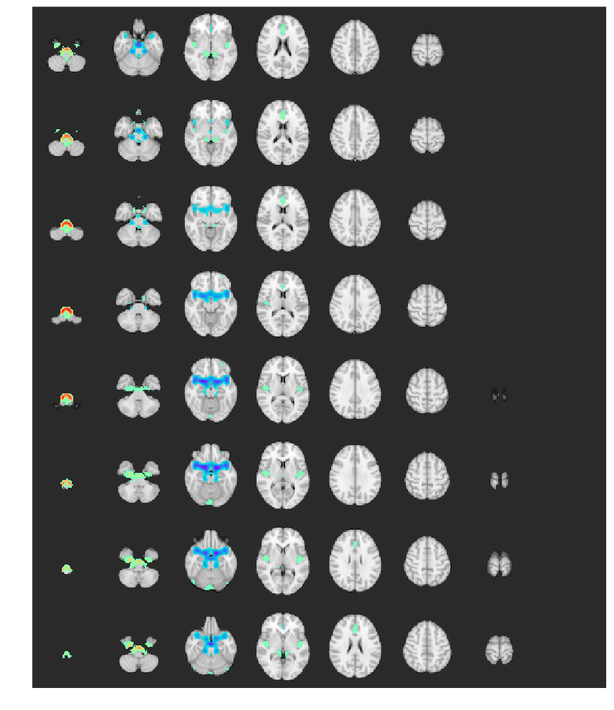
Figure 6.3: The component with lowest inter-subject weight correlation, where the accompanying spatial vector is weighted heavily toward the brain stem.

Two selected components from the final MCMC sample are visualised in Figure 6.2 and Figure 6.3. The latent spatial vectors are thresholded at $(2/V)\sum_{v}|\mathbb{S}_{k,v}|$ and overlaid on an anatomical reference image. The time courses for each subject are also visualised by slicing the $\mathbb{A}_{:,k}$ appropriately.

We can measure the correlation between different subject-wise time-series as a measure of synchronisation, which is often seen as indicative of a link to the experimental task. The component shown in 6.2 has a very high intra-subject correlation. Visual inspection of the spatial vector shows the component loads heavily on auditory regions as well as the parietal cortex. The accompanying subject-wise time series show a strong level of synchronisation. Hence this component is biologically plausible.

The feature in Figure 6.3 appears more like an artefact in the data and had the least synchronised set of time courses in the decomposition. We can see that the component primarily loads very heavily on the brain stem, and so is unlikely to relate meaningfully to the experimental task.

7 Discussion

We have extended methods for matrix factorisation with an unknown number of latent vectors. We imposed soft constraints on the regularity of latent features through a nondiagonal latent covariance structure. We provided a roadmap for combinining different forms of regularity constraints. We implemented in detail a model for smoothness of latent features expressed through an eigendecomposition based on the Discrete Cosine Transform. The method is general however, and for example, we could penalise activity in particular regions using the Discrete Wavelet Transform.

The model presented here also improves on previous work by allowing non-zero means for feature weights, which enables the learned feature vectors to explain variation seen in the data, rather than relying on covariance structure.

Section 5 demonstrated the benefits of this modelling strategy in a denoising example when the latent features were smooth 2D images. It was seen that this improved the mixing of the chain, recovered features closer to the ground truth, and removed noise more effectively than the prior used in previous work. As the latent activations were sparse we also compared our inferred weights to the output of FastICA, observing that the model presented here learned a more highly kurtotic weight distribution thus optimising this ICA proxy criterion more effectively.

In Section 6 we demonstrated these methods on a neuroimaging application. The efficient computational strategies introduced here for dealing with nondiagonal latent covariance were essential since numerical methods would fail on $V\times V$ matrices when $V>10^{5}$. We are not aware of other methods that are able to provide similar modelling capabilities at present.

8 Ackowledgements

This work was supported by the Medical Research Council [Unit Programme number U105292687]. The Cambridge Centre for Ageing and Neuroscience (Cam-CAN) research was supported by the Biotechnology and Biological Sciences Research Council (grant number BB/H008217/1).

References

- Ahmed et al. (1974) Nasir Ahmed, T_ Natarajan, and Kamisetty R Rao. Discrete cosine transfom. IEEE transactions on Computers, (1):90–93, 1974.
- Bengio et al. (2013) Yoshua Bengio, Aaron Courville, and Pascal Vincent. Representation learning: A review and new perspectives. IEEE transactions on pattern analysis and machine intelligence, 35(8):1798–1828, 2013.
- Bezanson et al. (2014) Jeff Bezanson, Alan Edelman, Stefan Karpinski, and Viral B Shah. Julia: A fresh approach to numerical computing. Technical report, 2014.
- Campbell et al. (2015) Karen L Campbell, Meredith A Shafto, Paul Wright, Kamen A Tsvetanov, Linda Geerligs, Rhodri Cusack, Lorraine K Tyler, et al. Idiosyncratic responding during movie-watching predicted by age differences in attentional control. Neurobiology of Aging, 2015.
- Elad et al. (2010) Michael Elad, Mario AT Figueiredo, and Yi Ma. On the role of sparse and redundant representations in image processing. Proceedings of the IEEE, 98(6):972–982, 2010.
- Griffiths and Ghahramani (2011) Thomas L Griffiths and Zoubin Ghahramani. The indian buffet process: An introduction and review. The Journal of Machine Learning Research, 12:1185–1224, 2011.
- Hyvärinen and Oja (2000) Aapo Hyvärinen and Erkki Oja. Independent component analysis: algorithms and applications. Neural networks, 13(4):411–430, 2000.
- Hyvärinen et al. (2009) Aapo Hyvärinen, Jarmo Hurri, and Patrick O Hoyer. Natural Image Statistics: A Probabilistic Approach to Early Computational Vision., volume 39. Springer Science & Business Media, 2009.