Cut moments approach in the analysis of DIS data

Abstract

We review the main results on the generalization of the DGLAP evolution equations within the cut Mellin moments (CMM) approach, which allows one to overcome the problem of kinematic constraints in Bjorken $x$. CMM obtained by multiple integrations as well as multiple differentiations of the original parton distribution also satisfy the DGLAP equations with the simply transformed evolution kernel. The CMM approach provides novel tools to test QCD; here we present one of them. Using appropriate classes of CMM, we construct the generalized Bjorken sum rule that allows us to determine the Bjorken sum rule value from the experimental data in a restricted kinematic range of $x$. We apply our analysis to COMPASS data on the spin structure function $g_{1}$.

I Introduction

In virtue of QCD factorization in hard processes hadron properties in the deep inelastic scattering (DIS) can be described in terms of the parton distribution functions (PDFs) $f_{p}(x,\mu^{2})$. They are universal process-independent densities explaining how the whole hadron momentum $P$ is partitioned in $x\cdot P$ between partons of type $p$. Here hard momentum transfer $q$: $-q^{2}=Q^{2}\gg P^{2}=m^{2}_{h}$, and the Bjorken variable $x$ satisfies $0<x=Q^{2}/(2Pq)<1$. These distributions $f_{p}(x,\mu^{2})$ are formed by nonperturbative strong interaction at hadronic scale $m^{2}_{h}$, while the dependence on the normalization scale $\mu^{2}$ is governed by the well-known Dokshitzer-Gribov-Lipatov-Altarelli-Parisi (DGLAP) evolution equations Gribov and Lipatov (1972a, b); Dokshitzer (1977); Altarelli and Parisi (1977) within perturbative QCD. Alternatively, one can study how to evolve with this scale $\mu^{2}$ the Mellin moments of the parton densities $f(n,\mu^{2})$, which are integrals of PDFs weighted with $x^{n}$ over the whole range (0,1) of $x$. These moments provide a natural framework of QCD analysis as they originate from the basic formalism of operator product expansion. However, these standard moments, in principle, cannot be extracted from any experiment due to kinematic constraints inevitably appearing in real DIS of lepton-hadron and hadron-hadron collisions. Namely, arbitrarily small values of the variable $x$ cannot be reached in experiments, which shows itself especially in “fixed target” experiments like in JLab Deur et al. (2008, 2014). It would be useful to invent new “real observables” with a goal to overcome the kinematic constraints. They were realized as the “cut (truncated) Mellin moments” (CMM) $\displaystyle f(z;n,\mu^{2})=\int^{1}_{z}f(x,\mu^{2})x^{n-1}dx$, generalized moments of the parton distribution $f(x,\mu^{2})$ in the unavoidable lower limit of integration $z\equiv x_{\text{min}}=Q^{2}_{\text{min}}/(2(Pq)_{\text{max}})>0$, and in this way the kinematic constraint can be taken into account. This circumstance can be the main reason for large uncertainties at data processing: this effect is aggravated if a singularity of $f(x,\mu^{2})$ in the neighborhood of $x=0$ is expected Deur et al. (2014).

The idea of “truncated” Mellin moments of the parton densities in QCD analysis was introduced and developed in the late 1990s Forte and Magnea (1999); Forte et al. (2001); Piccione (2001); Forte et al. (2002). The authors obtained the nondiagonal differential evolution equations, in which the $n$th truncated moment couples to all higher ones. Later on, diagonal integro-differential DGLAP-type evolution equations for the single and double truncated moments of the parton densities were derived in Kotlorz and Kotlorz (2007) and Kotlorz and Kotlorz (2009, 2011), respectively. The main finding of the truncated CMM approach is that the $n$th moment of the parton density also obeys the DGLAP equation, but with a rescaled evolution kernel $P^{\prime}(z)=z^{n}P(z)$ Kotlorz and Kotlorz (2007). The CMM approach has already been successfully applied, e.g., in spin physics to derive a generalization of the Wandzura-Wilczek relation in terms of the truncated moments and to obtain the evolution equation for the structure function $g_{2}$ Kotlorz and Kotlorz (2011, 2014). The advantages of the CMM approach to QCD factorization for DIS structure functions were also presented in Kotlorz and Kotlorz (2016). The truncation of the moments in the upper limit is less important in comparison to the low-$x$ limit because of the rapid decrease of the parton densities as $x\rightarrow 1$; nevertheless, a comprehensive theoretical analysis requires an equal treatment of both truncated limits. The evolution equations for double cut moments and their application to study the quark-hadron duality were also discussed in Psaker et al. (2008). Recently, a valuable generalization of the CMM approach incorporating multiple integrations as well as multiple differentiations of the original parton distribution has been obtained Kotlorz and Mikhailov (2014). This novel generalization of CMM and the corresponding DGLAP equations provides a powerful tool to test QCD at experimental constraints. In Sec. II, we briefly discuss the approach and present its main practically important results together with its DGLAP evolution. Then we focus attention on a new important special CMM. Based on this CMM, we construct in Sec. III a device to improve an experimental determination of the Bjorken polarized sum rule. In Sec. IV, we present the simplified form of the effective method, based on the CMM, for practical use in analysis of data. We apply it to the COMPASS measurements on $g_{1}$ Adolph et al. (2016) and also discuss the impact of the higher twist effects using Jlab data.

II CMM as solutions of DGLAP generalization

To apply our approach to specific cases of cut Mellin moments, like the Bjorken polarized sum rule (BSR), we consider it in more general context, as solutions of the DGLAP evolution Kotlorz and Mikhailov (2014). Indeed, to deal with new distributions CMM to process DIS data, one should know how the CMM can be evolved with the factorization scale $\mu^{2}$. We review here a variety of linear transformations $\hat{L}$ under the solutions of the nonsinglet DGLAP equation that lead to generalized CMM (gCMM) and then focus our attention on special cases of gCMM. Suppose $f(x,\mu^{2})$ is a solution of the nonsinglet DGLAP equation with the kernel $P(y,a_{s}(\mu^{2}))$,

$$\dot{f}\equiv\frac{d}{d\ln\mu^{2}}f(z,\mu^{2})=(P\ast f)(z)\equiv\int\limits_{0}^{1}P(y,a_{s}(\mu^{2}))\;f(x,\mu^{2})\;\delta(z-xy)\;dx\,dy,$$ (1)

where the sign $\ast$ means Mellin convolution; the running coupling $a_{s}=\alpha_{s}/(4\pi)$ satisfies the renormalization group equation with the QCD $\beta$ function in the rhs $\displaystyle\mu^{2}\frac{d}{d\mu^{2}}a_{s}(\mu^{2})=-\beta\left(a_{s}(\mu^{2})\right)$. Then the linear transformed $f$, $f\to{\cal F}=\hat{L}f$, which is a generalization of CMM (see the second column of Table 1) is also the solution of the DGLAP equation:

$$\dot{{\cal F}}=({\cal P}\ast{\cal F})$$ (2a)

with the kernel $${\cal P}$$,

$${\cal P}(y,a_{s}(\mu^{2}))=\hat{L}P(y,a_{s}(\mu^{2}))\hat{L}^{-1},~{}\text{where}~{}\hat{L}\ast\hat{L}^{-1}=\delta(1-y)\,.$$ (2b)

No.	Generalized CMM ${\cal F}$	DGLAP Kernel ${\cal P}$
1.	$f(x)$	$P(y)$
2.	$x^{n}f(x)$	$P(y)\cdot y^{n}$
3.	$f(z;n)=\int_{z}^{1}x^{n-1}\,f(x)\,dx$	$P(y)\cdot y^{n}$
4.	$f(z;\{n_{i}\}_{k})=\int\limits_{z}^{1}z_{k}^{n_{k}-1}dz_{k}\int\limits_{z_{k}}^{1}z_{k-1}^{n_{k-1}-1}dz_{k-1}\>...\int\limits_{z_{2}}^{1}z_{1}^{n_{1}-1}\;f(z_{1},\mu^{2})\;dz_{1}\,$	$\displaystyle P(y)\cdot y^{\sum_{i=1}^{k}n_{i}}$
5.	$\displaystyle f(z;\{n,0\}_{\nu})=\int_{z}^{1}\frac{\ln^{(\nu-1)}\left(x/z\right)}{\Gamma(\nu)}~{}x^{n}f(x)\,\frac{dx}{x}$	$P(y)\cdot y^{n}$
6.	$\displaystyle f(z;\{n,1\}_{\nu})=\int_{z}^{1}\frac{(x-z)^{\nu-1}}{\Gamma(\nu)}\,~{}x^{n}f(x)\,\frac{dx}{x}$	$P(y)\cdot y^{n+\nu-1}$
7.	$\displaystyle-\frac{df(x)}{dx}$	$P(y)\cdot y^{-1}$
8.	$\displaystyle\left(-\frac{d}{dx}\right)^{k}\left[x^{n}f(x)\right]$	$P(y)\cdot y^{n-k}$
9.	$\displaystyle f(z;*\omega)=(\omega\ast f)(z)$	$P(y)$

Table 1: Collection of the main results of CMM generalization of the DGLAP equations. The second column contains the generalized CMM ${\cal F}$ and the third column contains corresponding DGLAP evolution kernels ${\cal P}$.

The different transformations $\hat{L}$ are presented in Table 1 explicitly: in the second column—for ${\cal F}$, in the third one—for the corresponding DGLAP evolution kernel ${\cal P}$. Item 4 lays the key role: all the other results below can be obtained from this ${\cal F}$. They admit generalization from integer $k$ to real $\nu$ for items 5, 6, and 8; see the discussion in Kotlorz and Mikhailov (2014). The partial solutions in 7 and 8 were also considered earlier in Teryaev (2005); Artru et al. (2009). The expression in item 5 admits differentiation and integration with respect to the parameter $\nu$ and leads to new solutions. The same is also true for the expression in item 6 with the evident additional modification of the kernel $P$ and the convolution in the right-hand side of the DGLAP equation. Based on these gCMM, different interesting special solutions of the generalized DGLAP equations (2) can be constructed and applied to an analysis of the experimental data.

It is evident that the singlet case keeps in force the same transformations $\hat{L}$ under the quark $q(x,Q^{2})$ and gluon $g(x,Q^{2})$ distributions simultaneously and, respectively, (2b) under the matrix of the corresponding evolution kernels. In other words, Eq. (1) can be extended to a homogeneous system of evolution equations together with symmetry transformations in Eq. (2).

Now let us focus on the transform in item 5 in Table I. The corresponding DGLAP kernel for it is independent of $\nu$. Hence, integrands $\ln^{k}\left(x/z\right)/k!$ at different $k$ are “bricks” for any new gCMM constructions that evolve following the DGLAP equation with the same kernel $P$. Indeed, for any normalized weight $\omega(t)$ the CMM $f(x;*\omega)$, presented as a Mellin convolution of PDFs $f$ and $\omega$ (see item 9 of Table 1),

$$f(x)\to{\cal F}(x)\equiv f(x;*\omega)=\left(\omega\ast f\right)(x) \equiv \int_{x}^{1}\omega\left(x/z\right)~{}f(z,\mu^{2})\,\frac{dz}{z},$$ (3b)

$$\int_{0}^{1}\omega(t)dt=1\,,$$

is normalized as $f$,

$$\int_{0}^{1}f(x;*\omega)\,dx=\int_{0}^{1}f(x)\,dx=1.$$ (4)

The corresponding DGLAP kernel ${\cal P}$ for the $f(x;*\omega)$ can be obtained directly in virtue of the commutativity of Mellin convolution, ${\cal P}=\omega\ast P\ast\omega^{-1}=P$ . The weight $\omega(t)$ can be considered as a result of appropriate (including infinite) sums of the mentioned normalized bricks $\ln^{k}\left(t\right)/k!$; each of them does not change the DGLAP kernel. To return to the initial PDF $f(x)$, one must take $\omega(z)=\delta(1-z)$ in the definition (3). We shall investigate the applications of these properties for experimental data analysis in the case of the nonsinglet spin structure function $g_{1}~{}$ (in other notation $g_{1}^{NS}$) in the next sections.

III Generalized Bjorken sum rule

We construct the generalized truncated moment $g_{1}(z,n,\omega)$ as a Mellin convolution of the function $g_{1}$ with any normalized function $\omega(x)$, Eq. (3b), which obeys the DGLAP evolution equation with the rescaled kernel:

$$g_{1}(x,n;\omega)=\int_{x}^{1}\omega\left(x/z\right)\,g_{1}(z)\,z^{n}\,\frac{dz}{z}\,,$$ (5)

$${\cal P}(y)=P(y)\cdot y^{n}.$$ (6)

For $n=0$ one obtains

$$g_{1}(x,0;\omega)=\left(\omega\ast g_{1}\right)(x)$$ (7)

with the same evolution kernel as $g_{1}$, namely $P(y)$. In this way, we define the cut Bjorken sum rules, $\Gamma_{1}(x_{0})$, and simultaneously, the generalized cut Bjorken sum rules (gBSR), $\Gamma_{1;\omega}(x_{0})$,

$$\Gamma_{1}(x_{0}) = \int_{x_{0}}^{1}g_{1}(x)\,dx\,,$$ (8)

$$\Gamma_{1;\omega}(x_{0}) = \int_{x_{0}}^{1}g_{1}(x,0;\omega)\,dx,$$ (9)

which are equal to the ordinary Bjorken sum rule as $x_{0}\to 0$:

$$\Gamma_{1;\omega}(0)=\int_{0}^{1}g_{1}(x,0;\omega)\,dx=\int_{0}^{1}g_{1}(x)\,dx\equiv\Gamma_{1}(0).$$ (10)

We shall estimate the value of $\Gamma_{1}(0)$ from the smooth extrapolation of the truncated moments $\Gamma_{1;\omega}(x_{0})$ in $x_{0}$. To this aim, we construct a bunch of different $\Gamma_{1;\omega}(x_{0})$. Note that $\Gamma_{1;\omega}(x_{0})\leqslant\Gamma_{1}(x_{0})$ for any non-negative $\omega$ that leads to one-side estimates $\Delta=\Gamma_{1}(x_{0})-\Gamma_{1;\omega}(x_{0})\geqslant 0$. To extend the range of variation of the approach and enable upper estimates of $\Gamma_{1}(x_{0})$, we construct a bunch of $\Gamma_{1;\omega}(x_{0})$ based on the simple sign-changing normalized function $\omega(x)$ depending on three parameters $z_{1},~{}z_{2},~{}A$,

$$\omega(z)=-A\,\delta(z-z_{1})+(1+A)\,\delta(z-z_{2}).$$ (11)

Here the $\omega$-model parameters are $z_{2}>z_{1}>x_{0}>0$ and $A>0$ for the sign change. This model, following (7), leads to a “shuffle” of the initial PDF $g_{1}$ with different weights and arguments:

$$g_{1}(x,0;\omega)=-A\frac{\theta(z_{1}>x)}{z_{1}}g_{1}(x/z_{1})+(1+A)\frac{\theta(z_{2}>x)}{z_{2}}g_{1}(x/z_{2})\,,$$ (12)

$$\Gamma_{1;\omega}(x_{0})=\int_{x_{0}/z_{2}}^{1}\,g_{1}(x)\,dx+A\,\int_{x_{0}/z_{2}}^{x_{0}/z_{1}}\,g_{1}(x)\,dx.$$ (13)

The $\Gamma_{1;\omega}(x_{0})$ approaches $\Gamma_{1}(x_{0})$ from above, $\Gamma_{1;\omega}(x_{0})\geqslant\Gamma_{1}(x_{0})$ for

$$A>\int_{x_{0}}^{x_{0}/z_{2}}\,g_{1}(x)\,dx\,\Big{/}\int_{x_{0}/z_{2}}^{x_{0}/z_{1}}\,g_{1}(x)\,dx.$$ (14)

We shall fit free $\omega$-model parameters in order to saturate the integral $\Gamma_{1;\omega}(x_{0})$ as soon as possible when the parameter $x_{0}$ tends to $0$. To this end, let us expand $\Gamma_{1;\omega}(0)$ into Taylor series around $x_{0}$,

$$\Gamma_{1}(0)=\Gamma_{1;\omega}(x_{0}-x_{0})=\Gamma_{1;\omega}(x_{0})-x_{0}\,\Gamma^{\prime}_{1;\omega}(x_{0})+x_{0}^{2}\,\frac{1}{2}\,\Gamma^{\prime\prime}_{1;\omega}(x_{0})+\cdots\,,$$ (15)

to estimate $\Gamma_{1}(0)$ in the lhs using a few first orders of Taylor expansion in the rhs of Eq. (15). Requiring the first derivatives to vanish, $\Gamma^{\prime}_{1;\omega}(x_{0})=0$, or, requiring the same for the second one, $\Gamma^{\prime\prime}_{1;\omega}(x_{0})=0$, to straighten the behavior of $\Gamma_{1;\omega}(x_{0})$, one can improve the approach to $\Gamma_{1}(0)$.

(1) Let us require $\Gamma^{\prime}_{1;\omega}(x_{0})=0$, then for the lhs of Eq. (15) one obtains the approximation:

$$\Gamma_{1}(0)\approx\Gamma^{\rm{0APX}}_{1}(x_{0})=\Gamma_{1;\omega}(x_{0})+0+\frac{1}{2}\,x_{0}^{2}\,\Gamma^{\prime\prime}_{1;\omega}(x_{0}).$$ (16)

This condition fixes the value of the model parameter $A=A_{01}(x_{0})$ and then $\Gamma^{\prime\prime}_{1;\omega}(x_{0})$:

$$A_{01}(x_{0}) = \left[\frac{t_{1}\,g_{1}(t_{1})}{t_{2}\,g_{1}(t_{2})}-1\right]^{-1}\,,$$ (17)

$$x_{0}^{2}\,\Gamma^{\prime\prime}_{1;\omega}(x_{0}) = A_{01}(x_{0})\,t_{1}^{2}\,g^{\prime}_{1}(t_{1})-\left[1+A_{01}(x_{0})\right]t_{2}^{2}\,g^{\prime}_{1}(t_{2}),$$ (18)

where here and below $\displaystyle t_{1}=\frac{x_{0}}{z_{1}},~{}t_{2}=\frac{x_{0}}{z_{2}}$. For a special (single) root $x_{0}=x_{00}$ that satisfies the condition

$$\frac{1}{z_{1}}\,\frac{g^{\prime}_{1}(t_{1})}{g_{1}(t_{1})}=\frac{1}{z_{2}}\,\frac{g^{\prime}_{1}(t_{2})}{g_{1}(t_{2})},$$ (19)

the second derivation $\Gamma^{\prime\prime}_{1;\omega}(x_{00})$ vanishes also and the approximation $\Gamma^{\rm{0APX}}_{1}(x_{0})$ in (16) in this case reduces to

$$\Gamma_{1}(0)\approx\Gamma^{\rm{0APX}}_{1}(x_{00})+0+0$$ (20)

with $A_{00}=A_{01}(x_{00})$.

(2) Let us require now $\Gamma^{\prime\prime}_{1;\omega}(x_{0})=0$, which leads to the first order approximation (IAPX),

$$\Gamma_{1}(0)\approx\Gamma^{\rm{IAPX}}_{1}(x_{0})=\Gamma_{1;\omega}(x_{0})-x_{0}\,\Gamma^{\prime}_{1;\omega}(x_{0})+0,$$ (21)

with $A=A_{02}(x_{0})$ and $\Gamma^{\prime}_{1;\omega}(x_{0})$:

$$A_{02}(x_{0}) = \left[\frac{t_{1}^{2}\,g_{1}^{\prime}(t_{1})}{t_{2}^{2}\,g^{\prime}_{1}(t_{2})}-1\right]^{-1}\,,$$ (22)

$$x_{0}\,\Gamma^{\prime}_{1;\omega}(x_{0}) = A_{02}(x_{0})\,t_{1}\,g_{1}(t_{1})-\left[1+A_{02}(x_{0})\right]t_{2}\,g_{1}(t_{2}).$$ (23)

To illustrate the features of $\Gamma_{1;\omega}$, we plot the bunch $\Gamma_{1;\omega}(x_{0})$ in Eq. (13) for different values of $A$ in Figs. 1 and 2, including: “constant behavior” value $A=A_{00}=A_{01}(x_{00})$ fixed at special root $x_{00}\approx 0.037$, “quasilinear behavior” value $A=A_{02}(\bar{x})$ fixed at some value $\bar{x}=0.01$ (22), and the standard truncated Bjorken sum rule $\Gamma_{1}(x_{0})$, Eq. (8) (thick black curve).

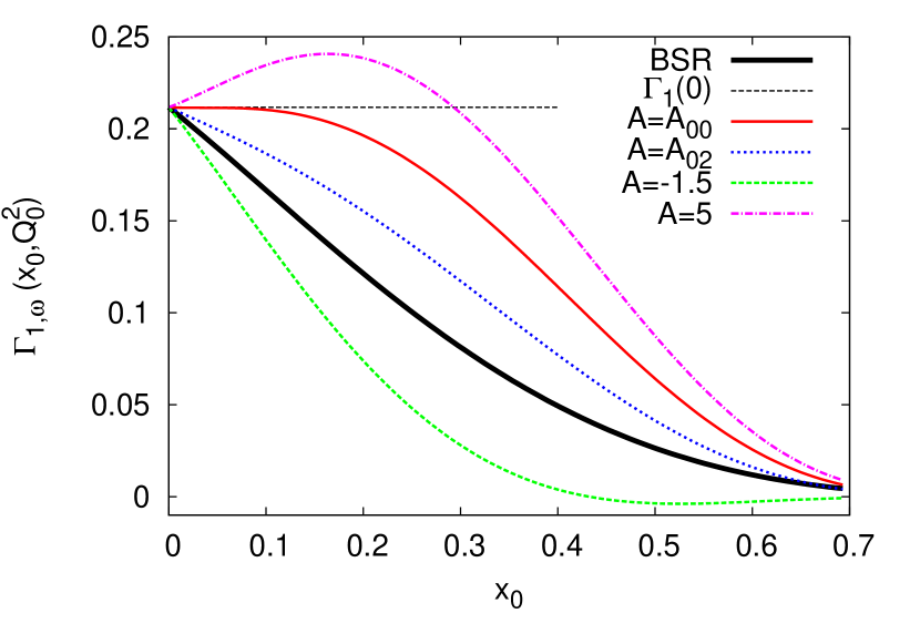
Figure 1: $\Gamma_{1;\omega}(x_{0})$, Eq. (13), for different values of $A$ and the truncated BSR $\Gamma_{1}(x_{0})$, Eq. (8) (thick black curve) as a function of $x_{0}$. Input parametrization, Eq. (24), with $a=0$.

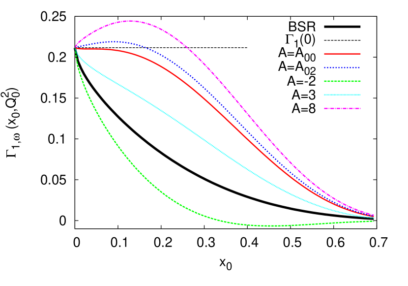
Figure 2: $\Gamma_{1;\omega}(x_{0})$, Eq. (13), for different values of $A$ and the truncated BSR $\Gamma_{1}(x_{0})$, Eq. (8) (thick black curve) as a function of $x_{0}$. Input parametrization, Eq. (24), with $a=-0.4$.

One can see that an appropriate model of $g_{1}$ shuffling can improve significantly the approach $\Gamma_{1;\omega}(x_{0})$ to $\Gamma_{1}(0)$; see, e.g., the red curve for $A=A_{00}$. The parameters of an optimal $\omega$ depend on the behavior of $g_{1}(x)$ (especially in the neighborhood of zero), which is fixed by different input parametrizations of $g_{1}$ at $Q_{0}^{2}=1\,\rm{GeV^{2}}$,

$$g_{1}(x,Q_{0}^{2})=N\cdot x^{a}(1-x)^{b}(1+\gamma x),$$ (24)

where $a=0$ in Fig. 1 and $a=-0.4$ in Fig. 2, respectively, at $b=3$, $\gamma=5$ and the coefficient $N$ is the norm. In our tests, in order to obtain a smooth approach of the bunch in the experimentally available $x$ region, we fixed $z_{1}=0.7$ and $z_{2}=0.9$. The already mentioned root $x_{00}\approx 0.037$ for the parametrization, Eq. (24) ($x_{00}$ value does not depend on the $a$ parameter of the input), corresponds to approximation (20). It is important to mention that the quasilinear regime near $0$ visibly starts at rather large values of $x_{0}\gtrsim 0.1$ for the different parametrization in (24). This should ensue the applicability of approximation (21) even for JLab experimental conditions, where the admissible $x$ bunches are rather far from 0. In practice, one can use fit to the data instead of the ready input parametrization. It is worthy to notice that the analysis based on the bunch behavior allows one to shift the available region of $x$ to smaller values, $x_{0}=x\cdot z_{2}$. In this manner, using data from large $x$ and choosing suitable values of $z_{1}$ and $z_{2}$, one is able to get an answer in a much smaller $x$ region.

In this section, we have shown in detail how to construct the generalized Bjorken sum rule and illustrated the mechanism of shuffling in it. We have also presented different methods of estimation of $\Gamma_{1}(0)$ within the gBSR approach. In the next section, we shall present the simplified form of the most important equations of our approach, rewritten in terms of experimental parameters, for practical use in analysis of data.

IV Practical analysis of data

The generalized Bjorken sum rule enables one to analyze integrals over the experimentally accessible $x$ range in a manner in which $\Gamma_{1;\omega}(x_{0})>\Gamma_{1}(x_{0})$. In this way, for $x_{0}>0$, $\Gamma_{1;\omega}(x_{0})$, Eq. (9) approaches $\Gamma_{1}(0)$ closer than the original BSR $\Gamma_{1}(x_{0})$, Eq. (8). For practical purposes, we rewrite here the essential formulas from the previous section in terms of experimental data and demonstrate the effective method for the estimation of $\Gamma_{1}(0)$. Thus, the gBSR, Eq. (13), where the lower limit of integrations has to be strictly related to the minimal $x$ accessible experimentally, $x_{min}$, takes the form

$$\Gamma_{1;\omega}(x_{min},r)=\int_{x_{min}}^{1}\,g_{1}(x)\,dx+A\,\int_{x_{min}}^{x_{min}/r}\,g_{1}(x)\,dx.$$ (25)

The experimental lower value $x_{min}$ in the above equation is related to $x_{0}$ from Eq. (13) via $x_{0}=x_{min}\cdot z_{2}$. The ratio parameter, $r\equiv z_{1}/z_{2}$,

$$x_{min}\,<\,r\,<\,1\,,$$ (26)

can also be chosen taking into account the set of experimental $x$ points. Please note that in the above formulas $x_{0}$ and $z_{2}$ do not appear separately, only as a ratio, $x_{0}/z_{2}=x_{min}$. It means that gBSR can mimic a shift of the argument of the original BSR, $\Gamma_{1}(x_{min})$ to the smaller one, $\Gamma_{1}(x_{0})$.

We have tested the methods of estimation of $\Gamma_{1}(0)$, described in Sec. III and have found that a very effective method, universal for the different small-$x$ behavior of $g_{1}$ and for $x_{min}\lesssim 0.1$, is the first order approximation, Eqs. (21) and (22). With use of the experimental parameters $x_{min}$ and $r$, it reads

$$\Gamma_{1}(0)\approx\Gamma^{\rm{IAPX}}_{1}(x_{min},r)=\Gamma_{1;\omega}(x_{min},r)+(A+1)\,x_{min}\,g_{1}(x_{min})-A\frac{x_{min}}{r}g_{1}(x_{min}/r)$$ (27)

with

$$A=\left[r^{2}\,\frac{g^{\prime}_{1}(x_{min}/r)}{g^{\prime}_{1}(x_{min})}-1\right]^{-1}$$ (28)

and $\Gamma_{1;\omega}(x_{min},r)$ given in Eq. (25). $\Gamma_{1}(0)$ from Eq. (27) can be compared to the estimate from the original BSR $\Gamma_{1}(x_{min})$, (8), in the same first order approximation,

$$\Gamma_{1}(0)\approx\Gamma^{\rm{IBSR}}_{1}(x_{min})=\Gamma_{1}(x_{min})+x_{min}\,g_{1}(x_{min}).$$ (29)

In Fig. 4, we plot the percent errors $\epsilon^{\text{I}}(x_{min},r)$,

$$\epsilon^{\text{I}}(x_{min},r)=\left(\Gamma_{1}(0)-\Gamma^{\text{IAPX}}_{1}(x_{min},r)\right)/\Gamma_{1}(0)*100\%$$ (30)

as a function of $x_{min}$ for three values of the ratio $r$. We assume a not too singular small-$x$ behavior of $g_{1}$, $a=-0.1$ in Eq. (24). In Fig. 4 we present the same but for a rather singular shape of $g_{1}$, $a=-0.4$. For comparison, in both figures we show also the large error $\epsilon^{\text{IBSR}}(x_{min})$,

$$\epsilon^{\text{IBSR}}(x_{min})=\left(\Gamma_{1}(0)-\Gamma^{\text{IBSR}}_{1}(x_{min})\right)/\Gamma_{1}(0)*100\%\,.$$ (31)

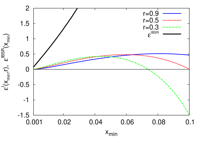
Figure 3: The percent errors $\epsilon^{\text{I}}(x_{min},r)$, Eq. (30), for different $r:0.9,0.5,0.3$, together with $\epsilon^{\text{IBSR}}(x_{min})$, Eq. (31), as a function of $x_{min}$. Small-$x$ behavior of $g_{1}$ with $a=-0.1$, Eq. (24).

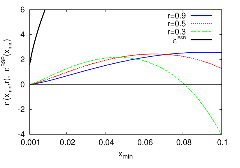
Figure 4: The percent errors $\epsilon^{\text{I}}(x_{min},r)$, Eq. (30), for different $r:0.9,0.5,0.3$, together with $\epsilon^{\text{IBSR}}(x_{min})$, Eq. (31), as a function of $x_{min}$. Small-$x$ behavior of $g_{1}$ with $a=-0.4$, Eq. (24).

The range of $x_{min}$ in our plots covers the smallest $x$ available in the polarized experiments $\sim$ 0.004 at COMPASS, 0.02 at HERMES, and 0.1 at Jlab. One can see a very good agreement of the estimated $\Gamma_{1}(0)$ with its true leading order (LO) value (assuming $g_{A}/{g_{V}}=1.27$), for not too singular behavior of $g_{1}$ at small $x$, independently of the ratio $r$. For more singular behavior of $g_{1}$, this agreement is still satisfactory and for $x_{min}\gtrsim 0.05$ it can be improved by taking the ratio parameter $r$, Eq. (26), as large as possible.

In Figs. 6 and 6, we present our results on determination of the BSR based on the COMPASS Adolph et al. (2016) data, where $x_{min}=0.0036$. We follow the method described above using Eqs. (25)—(28). We assume the input parametrization, Eq. (24), from our fit to the data at $Q^{2}=3$ GeV²: $g_{1}\sim x^{-0.42}(1-x)^{2.7}(1+3.4\,x)$.

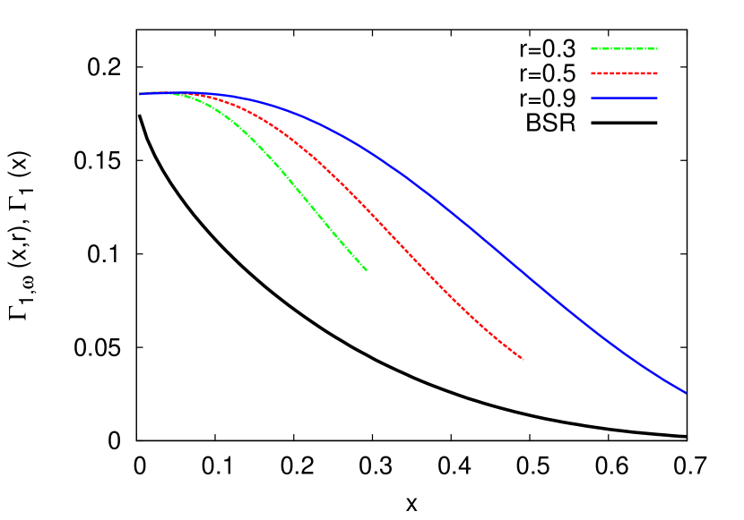
Figure 5: $\Gamma_{1,\omega}(x,r,Q^{2})$, Eq. (25), for $A(x_{min}=0.0036,r)$, Eq. (28) for three values of $r:0.9,0.5,0.3$, together with the truncated Bjorken sum rule $\Gamma_{1}(x,Q^{2})$, Eq. (8), as a function of $x$. The results are based on our fit to the COMPASS data.

Figure 6: The percent errors $\epsilon^{\text{I}}(r)$, Eq. (30), for $x_{min}=0.0036$, as a function of $r$. The results are based on our fit to the COMPASS data.

We find the following results for $x_{min}$ and different $r$:

$$\begin{array}[]{c|ccc|ccc}\Gamma_{1}(0)&r&\Gamma_{1}^{\text{IAPX}}&~{}\epsilon^{\text{I}}[\%]{}&r&\Gamma_{1}^{\text{IAPX}}&~{}\epsilon^{\text{I}}[\%]\\ \hline\cr 0.186&~{}0.1&0.185&1.4\cdot 10^{-2}&~{}0.9&0.186&-7.7\cdot 10^{-3}\end{array}$$

One can see that for the first order $\Gamma^{\rm{IAPX}}_{1}(x_{min},r)$ approximation the percentage error $\epsilon^{\text{I}}(x_{min}=0.0036)$, Eq. (30), is smaller than $1\%$ in the wide range $r>0.01$ and negligibly small for $r>0.05$. These results, together with the accuracy estimates presented in Figs. 4 and 4, confirm the efficiency of our integral transform $\omega$ to estimate the BSR.

These estimates can be compared with the QCD result for the BSR obtained in the $\overline{\rm MS}$ scheme in $O(\alpha_{s}^{n})$, $n=1,2,3$ and $4$ approximation in Kodaira et al. (1979); Gorishnii and Larin (1986); Larin and Vermaseren (1991) and Baikov et al. (2010), respectively, and incorporating higher twist (HT) effects,

$$\Gamma_{1}(Q^{2})=\frac{1}{6}\,\frac{g_{A}}{g_{V}}\left[\,1-\frac{\alpha_{s}}{\pi}-3.58\left(\frac{\alpha_{s}}{\pi}\right)^{2}-20.22\left(\frac{\alpha_{s}}{\pi}\right)^{3}-175.7\left(\frac{\alpha_{s}}{\pi}\right)^{4}\right]+\frac{\mu_{4}^{p-n}}{Q^{2}}\,.$$ (32)

Here $\alpha_{s}\equiv\alpha_{s}(Q^{2})$ is the running QCD coupling, the coefficients of expansion are taken for the number of active quarks $n_{f}=3$, and $\mu_{4}^{p-n}$ is the scale of the first power correction to the HT. The HT effects become essential in the small/moderate $Q^{2}$ region; see the analysis of its impact for BSR in Pasechnik et al. (2010). In our analysis $Q^{2}$ is of the order of a few $\rm{GeV}^{2}$ and the HT impact is visible, which is shown in Fig. 8.

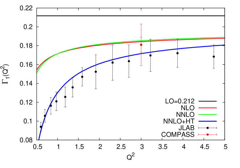
Figure 7: $\Gamma_{1}(Q^{2})$, Eq. (32), incorporating N²LO and HT corrections, $\mu_{4}^{p-n}/M^{2}=-0.047$, $\Lambda_{\text{qcd}}=311$ MeV, together with Jlab data Deur et al. (2014): black point, the single red point higher is the COMPASS result $0.181\pm 0.008\>{\rm stat.}\pm 0.014\>{\rm syst.}$ Adolph et al. (2016), $M$ is the nucleon mass.

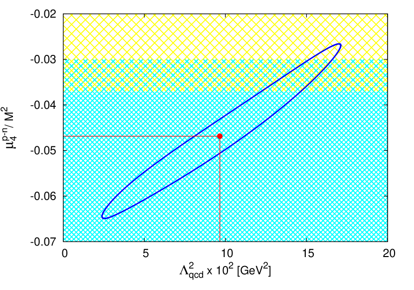
Figure 8: Contour plot of 1$\sigma$ error ellipse for $\Lambda^{2}_{\text{qcd}}$ and $\mu_{4}^{p-n}$, at the central point $\chi^{2}_{\text{ndf}}=0.60$. The upper band (yellow strip) represents the Jlab result $\mu_{4}^{p-n}/M^{2}=-0.021\pm 0.016$ Deur et al. (2014) and the lower band (blue strip) is a typical theoretical estimation, $\mu_{4}^{p-n}/M^{2}=-0.05\pm 0.02$ Pasechnik et al. (2010).

To illustrate the reasonableness of the new estimates for $\Gamma_{1}(Q^{2})$, we have processed the JLab results Deur et al. (2014) following Eq. (32) taken at N²LO, i.e., holding the first three terms in the perturbation part there. The results of the fit are shown in Figs. 8 and 8. In Fig. 8, we present 1$\sigma$ error ellipse for two adjusted fit parameters: $\Lambda_{\text{qcd}}=311\pm{}^{103}_{156}$ MeV and HT $\mu_{4}^{p-n}/M^{2}=-0.047\pm{}^{0.020}_{0.018}$; $M$ is the nucleon mass. These values look reasonable in view of the actual world average data: $\Lambda_{\text{qcd}}=332\pm 17$ MeV Patrignani et al. (2016) and $\mu_{4}^{p-n}/M^{2}=-0.05\pm 0.02$ Pasechnik et al. (2010), Deur et al. (2014).

V Conclusions

The QCD analysis of real data for the deep inelastic scattering processes faces the principal problem: Bjorken variable $x$ is constrained by the unavoidable kinematic condition (from below) $x\geqslant x_{\text{min}}=Q^{2}_{\text{min}}/(2(Pq)_{\text{max}})>0$. This is important for data processing, especially for the case of PDF $f_{p}(x,\mu^{2})$ increasing as $x\to 0$. The CMM approach has been elaborated just to overcome this problem. In this paper, we have reviewed the main results of the CMM approach and suggested its generalization that allows one to study the fundamental integral characteristics of the parton distributions in an experimentally restricted region of $x$. We demonstrated how, with the help of the so-called generalized Bjorken sum rule, one can determine the BSR $\Gamma_{1}$ from experimental data in the available $x$ region. We applied our approach to the COMPASS data and obtained good agreement with the QCD predictions for the BSR, incorporating higher twist effects estimated from the Jlab measurements. Concluding, the presented method seems to be promising in the analysis of the QCD sum rules.