Importance of ⁵⁶Ni production on diagnosing explosion mechanism of core-collapse supernova

Abstract

⁵⁶Ni is an important indicator of the supernova explosions, which characterizes light curves. Nevertheless, rather than ⁵⁶Ni, the explosion energy has often been paid attention from the explosion mechanism community, since it is easier to estimate from numerical data than the amount of ⁵⁶Ni. The final explosion energy, however, is difficult to estimate by detailed numerical simulations because current simulations cannot reach typical timescale of saturation of explosion energy. Instead, the amount of ⁵⁶Ni converges within a short timescale so that it would be a better probe of the explosion mechanism. We investigated the amount of ⁵⁶Ni synthesized by explosive nucleosynthesis in supernova ejecta by means of numerical simulations and an analytic model. For numerical simulations, we employ Lagrangian hydrodynamics code in which neutrino heating and cooling terms are taken into account by light-bulb approximation. Initial conditions are taken from Woosley & Heger (2007), which have 12, 15, 20, and 25 $M_{\odot}$ in zero age main sequence. We additionally develop an analytic model, which gives a reasonable estimate of the amount of ⁵⁶Ni. We found that, in order to produce enough amount of ⁵⁶Ni, $\mathcal{O}(1)$ Bethe s^-1 of growth rate of the explosion energy is needed, which is much larger than that found in recent exploding simulations, typically $\mathcal{O}(0.1)$ Bethe s^-1.

1 Introduction

The important product of supernova nucleosynthesis is ⁵⁶Ni, which drives supernova brightness. A typical amount of ⁵⁶Ni by canonical supernovae is estimated as $\mathcal{O}(0.01)M_{\odot}$ (Hamuy, 2003; Smartt, 2009), which can be measured by exponential tail from the late light curve with low ambiguity. In contrast, the explosion energy, which has been used as an indicator of the explosion simulations, needs two observables (light curve and spectrum) to be estimated, since it is interfered by a product of ejecta mass and velocity. It implies that the amount of ⁵⁶Ni has a smaller systematic error compared to the explosion energy. Indeed, for SN 1998bw as an example, the estimated explosion energy ranges from 2 to 25 Bethe (1 Bethe $\equiv 10^{51}$ erg) (Höflich et al., 1999; Nakamura et al., 2001; Maeda et al., 2006), depending on details of radiation transfer simulations and the ejecta structure assumed in such models, and methods to derive the physical quantities from observables. On the other hand, the estimated amount of ⁵⁶Ni is converged between 0.2 and 0.4 $M_{\odot}$. In addition, production of ⁵⁶Ni has been suggested to be sensitive to the explosion mechanism, that is, the energy deposition rate rather than the total explosion energy itself (see, e.g. Maeda & Tominaga, 2009; Suwa & Tominaga, 2015).

The mechanism of supernova explosions is still under a thick veil, even though it has been already more than 80 years from the original idea by Baade & Zwicky (1934), more than 50 years from the first numerical simulation (Colgate & White, 1966), and more than 30 years from the first simulation of delayed explosion (Bethe & Wilson, 1985), which is the current standard scenario of supernova explosion mechanism.

After a few decades of unsuccessful explosion era (Rampp & Janka, 2000; Liebendörfer et al., 2001; Thompson et al., 2003; Sumiyoshi et al., 2005), we have some exploding simulations since Buras et al. (2006) (e.g. Marek & Janka, 2009; Suwa et al., 2010; Takiwaki et al., 2012; Müller et al., 2012; Bruenn et al., 2013; Nakamura et al., 2015; Lentz et al., 2015; Müller, 2015; Pan et al., 2016; O’Connor & Couch, 2015; Burrows et al., 2016), in which multidimensional hydrodynamics equations are solved simultaneously with spectral neutrino transport. However, most of simulations have been performed in two-dimension (with axial symmetry). Three-dimensional simulations without any spacial symmetry employed have shown worse results than two dimensional ones (Hanke et al., 2012; Couch, 2013; Takiwaki et al., 2014; Lentz et al., 2015), since three dimensional turbulence leads to an energy cascade from large scale to small scale (normal cascade), while two dimensional one makes it opposite (inverse cascade). It is known that a large scale, i.e. global, turbulence aids the explosion, so that some results from two-dimensional simulations might reflect a numerical artifact and these simulations might well overestimate the explosion energy.

The state-of-the-art simulations have shown slow increase of the explosion energy. As summarized in Table 1, the growing rate of the explosion energy is typically $\mathcal{O}(0.1)$ Bethe s^-1, especially for 3D simulations. Therefore, it can be argued that, by neutrino heating mechanism, these simulations require at least a few second to get a canonical explosion energy, i.e. 1 Behte. It should be noted that the explosion energy estimated in explosion simulations is not a direct observable, since there is bound (totally negative energy) material above the shock and it reduces the explosion energy when it is swept by the shock.

The explosion energy is related to the ⁵⁶Ni synthesis, since to synthesize ⁵⁶Ni the temperature needs to be $T\mathrel{\hbox{\hbox to0.0pt{\hbox{\lower 5.0pt\hbox{$\sim$}}\hss}\hbox{$>$}}}5\times 10^{9}$ K. The postshock temperature is scaled by the explosion energy as $T=1.33\times 10^{10}\,\mathrm{K}(r_{\mathrm{shock}}/1000\,\mathrm{km})^{-3/4}(E_{\mathrm{exp}}/1\,\mathrm{Bethe})^{1/4}$, where $r_{\mathrm{shock}}$ is the shock radius (Woosley et al., 2002). Therefore with $E_{\mathrm{exp}}=1\,\mathrm{Bethe}$, ⁵⁶Ni can be generated for $r_{\mathrm{shock}}\mathrel{\hbox{\hbox to0.0pt{\hbox{\lower 5.0pt\hbox{$\sim$}}\hss}\hbox{$<$}}}3700$ km. Since shock velocity $v_{s}$ is roughly $10^{4}$ km s^-1 after the onset of the explosion, it takes only a few hundred milliseconds to reach this radius. If the growth rate of the explosion energy is small and it takes a few second to achieve 1 Bethe, it is not trivial whether ⁵⁶Ni is synthesized by explosive nucleosynthesis in the ejecta.

In this paper, we investigate ⁵⁶Ni production as an indicator of the explosion mechanism. First we perform numerical simulations of supernova explosion in Section 2. By calibrating with numerical simulation data about shock and temperature evolution, we construct an analytic model that describes shock and temperature evolution, which are important ingredients of ⁵⁶Ni production, and give constraint on the growth rate of the explosion energy to synthesize enough ⁵⁶Ni in Section 3. This analytic model is useful to investigate ⁵⁶Ni production for a broader parameter space of both the explosion properties and progenitor structure. We summarize our results and discuss their implications in Section 4.

Table 1: Properties of recent explosion simulations

Author(s)	ZAMS mass a	$\dot{E}_{\mathrm{exp}}$ b
	($M_{\odot}$)	(Bethe s-1)
2D (axisymmetric)
Bruenn et al. (2016)	12, 15, 20, 25	1.5 – 3
Suwa et al. (2016)	12 – 100	0.5 – 0.7
Pan et al. (2016)	11, 15, 20, 21, 27	1 – 5
O’Connor & Couch (2015)	12, 15, 20, 25	0.5 – 1
Nakamura et al. (2016)	17	0.4
Summa et al. (2016)	11.2 – 28	1
Burrows et al. (2016)	12, 15, 20, 25	1 – 3
3D
Lentz et al. (2015)	15	0.2
Melson et al. (2015)	9.6	0.6
Müller (2015)	11.2	0.4
Takiwaki et al. (2016)	11.2, 27	0.4 – 2

^a Not only the mass, evolution codes are also different.

^b Note that these numbers are quite rough estimates in the early phase ($\sim 100$ ms after the onset of explosion) based on figures in the literature.

2 Numerical simulations

2.1 Method

We employ blcode, which is a prototype code of SNEC (Morozova et al., 2015) and a pure hydrodynamics code based on Mezzacappa & Bruenn (1993), as a base. It solves Newtonian hydrodynamics in Lagrange coordinate. Basic equations are given by

$$\frac{\partial r}{\partial M} =\frac{1}{4\pi r^{2}\rho},$$ (1)

$$\frac{Dv}{Dt} =-\frac{GM}{r^{2}}-4\pi r^{2}\frac{\partial P}{\partial M},$$ (2)

$$\frac{D\epsilon}{Dt} =-P\frac{D}{Dt}\left(\frac{1}{\rho}\right)+\mathcal{H}-\mathcal{C},$$ (3)

where $r$ is radius, $M$ is mass coordinate, $\rho$ is density, $v$ is radial velocity, $t$ is time, $G$ is the gravitational constant, $P$ is pressure, and $\epsilon$ is specific internal energy. $D/Dt$ means Lagrange derivative. Artificial viscosity by von Neumann & Richtmyer (1950) is employed to capture a shock. Neutrino heating and cooling are newly added in this work by a method used in the literature (e.g. Murphy & Burrows, 2008), in which neutrino cooling is given as a function of temperature and neutrino heating is a function of radius with a parametric neutrino luminosity. Heating term, $\mathcal{H}$, and cooling term, $\mathcal{C}$, are given as

$$\mathcal{H}= 1.544\times 10^{20}\,\mathrm{erg\,g^{-1}\,s^{-1}}$$

$$\times\left(\frac{L_{\nu_{e}}}{10^{52}\mathrm{erg\,s}^{-1}}\right)\left(\frac{r}{100\mathrm{km}}\right)^{-2}\left(\frac{T_{\nu_{e}}}{4\mathrm{MeV}}\right)^{2},$$ (4)

$$\mathcal{C}= 1.399\times 10^{20}\,\mathrm{erg\,g^{-1}\,s^{-1}}\left(\frac{T}{2\mathrm{MeV}}\right)^{6}.$$ (5)

Here, we fixed neutrino temperature as $T_{\nu_{e}}=4$MeV. In addition, we take into account these terms only in postshock regime. We do not take into account optical depth terms (see Nordhaus et al., 2010; Hanke et al., 2012) for simplicity. We modify inner boundary conditions so that the innermost mass element does not shrink within 50 km from the center to mimic the existence of a protoneutron star. The Helmholtz equation of state by Timmes & Arnett (1999) is used. Initial composition is used for equation of state.

Table 2: Precollapse properties of the SN progenitors from Woosley & Heger (2007)

Name	${M_{s=4}}^{a}$	${R_{M_{s=4}}}^{b}$	${\rho_{M_{s=4}}}^{c}$	${\xi_{M_{s=4}}}^{d}$	${\mu_{M_{s=4}}}^{e}$	${R_{{M_{s=4}}+0.1M_{\odot}}}^{f}$	${\rho_{M_{s=4}+0.1M_{\odot}}}^{g}$	${\xi_{M_{s=4}+0.1M_{\odot}}}^{h}$	${\mu_{M_{s=4}+0.1M_{\odot}}}^{i}$
	($M_{\odot}$)	(1000 km)	($10^{7}$ g cm-3)			(1000 km)	($10^{7}$ g cm-3)
WH07s12	1.530	2.813	0.168	0.544	0.084	4.655	0.035	0.350	0.048
WH07s15	1.818	3.770	0.129	0.482	0.116	4.924	0.051	0.390	0.079
WH07s20	1.824	2.654	0.268	0.687	0.119	3.646	0.133	0.528	0.112
WH07s25	1.901	2.803	0.317	0.678	0.157	3.771	0.131	0.531	0.118

^a Mass with $s=4k_{B}$ baryon^-1.

^b Radius with $s=4k_{B}$ baryon^-1.

^c Density with $s=4k_{B}$ baryon^-1.

^d Compactness parameter of ${M_{s=4}}$, see Eq. (6).

^e $\mu$ parameter determined by Eq. (7) in units of $M_{\odot}/1000$ km.

^f Radius with ${M_{s=4}+0.1M_{\odot}}$.

^g Density with ${M_{s=4}+0.1M_{\odot}}$.

^h Compactness parameter of ${M_{s=4}}+0.1M_{\odot}$.

ⁱ $\mu$ parameter of ${M_{s=4}}+0.1M_{\odot}$ in units of $M_{\odot}/1000$ km.

The initial conditions are the 12, 15, 20, and 25 $M_{\odot}$ models from Woosley & Heger (2007). Properties of the progenitor models are given in Table 2. In this table, we show mass coordinate, radius, and density at a mass coordinate which has $s=4k_{B}$ baryon^-1, since the current understanding of shock launch is that it is realized when a mass element with $s=4k_{B}$ baryon^-1 is accreting onto the shock. In the fifth column, we show the “compactness parameter” (O’Connor & Ott, 2011), which is defined as

$$\xi_{M}=\frac{M/M_{\odot}}{R(M)/1000\,\mathrm{km}},$$ (6)

where $R(M)$ is the radius of the sphere whose mass coordinate is $M$. According to O’Connor & Ott (2011), smaller values of $\xi_{M}$ are better for explosions, but note that they used $\xi_{2.5}$, which is different from our values. The sixth column gives $\mu_{M}$ (Ertl et al., 2016), which is defined as

$$\mu_{M}=\left.\frac{dM}{dr}\right|_{r=R(M)}=4\pi\rho R^{2}(M),$$ (7)

in units of $M_{\odot}/1000$ km. Note that Ertl et al. (2016) evaluated the value of $dM/dr$ by computing the numerical derivative at the mass shell where $s=4k_{B}$ baryon^-1 with a mass interval of $0.3M_{\odot}$. Here we instead simply use the second equality in equation (7) to compute $dM/dr$ analytically. They showed that for a given value of $M_{s=4}$, a smaller $\mu_{M}$ is better for an explosion. From seventh to tenth columns give the same quantities as ones from third to sixth columns, but different mass coordinate $M_{s=4}+0.1M_{\odot}$.

The mass cut is determined by $M_{s=4}-0.2M_{\odot}$. We employ 1000 grids with mass resolution of $10^{-3}M_{\odot}$ so that $1M_{\odot}$ is included in numerical regime. To check the impact of this choice, we additionally perform a simulation with a mass cut of $M_{s=4}-0.3M_{\odot}$ with 1100 grid points and find no significant difference from standard grid model. We also performed a simulation with 1500 grids points and with the same total mass (i.e. 33% better rezolution) and found no significant differences. Therefore, the numerical results that will be shown below are insensitive to numerical setup.

In the following, we use the so-called diagnostic explosion energy, which is defined as the integral of the sum of specific internal, kinetic, and gravitational energies over all zones, in which it is positive, as an approximate estimate of the explosion energy. Note that this energy is not direct observables, since there is bound (totally negative energy) material above the shock and it reduces the explosion energy when it is swept by the shock.

2.2 Results

Table 3: Summary of simulations

Name	progenitor	${L_{\nu_{e},52}}^{a}$	${t_{\mathrm{exp}}}^{b}$	${t_{T_{9}=5}}^{c}$	${E_{\mathrm{exp},T_{9}=5}}^{d}$	${\dot{E}_{\mathrm{exp,T_{9}=5}}\,}^{e}$	${E_{\mathrm{exp},1\mathrm{s}}}^{f}$	${M_{\mathrm{PNS}}}^{g}$	${M_{{}^{56}Ni}}^{h}$
		($10^{52}$ erg s-1)	(ms)	(ms)	(Bethe)	(Bethe s-1)	(Bethe)	($M_{\odot}$)	($M_{\odot}$)
WH07s12L1	WH07s12	1	—	—	—	—	—	—	—
WH07s12L2	WH07s12	2	553	97	0.093	0.950	0.147	1.527	0.023 – 0.047
WH07s12L3	WH07s12	3	361	130	0.230	1.769	0.478	1.456	0.068 – 0.098
WH07s12L4	WH07s12	4	233	149	0.366	2.447	0.981	1.315	0.097 – 0.226
WH07s15L2	WH07s15	2	—	—	—	—	—	—	—
WH07s15L3	WH07s15	3	580	135	0.166	1.230	0.164	1.820	0.060 – 0.079
WH07s15L4	WH07s15	4	409	151	0.358	2.362	0.502	1.737	0.086 – 0.135
WH07s15L5	WH07s15	5	267	160	0.481	3.007	1.057	1.648	0.107 – 0.196
WH07s20L2	WH07s20	2	—	—	—	—	—	—
WH07s20L3	WH07s20	3	307	197	0.344	1.752	0.575	1.806	0.118 – 0.151
WH07s20L4	WH07s20	4	249	175	0.392	2.238	0.791	1.769	0.110 – 0.166
WH07s20L5	WH07s20	5	236	169	0.458	2.709	1.042	1.736	0.107 – 0.196
WH07s25L2	WH07s25	2	—	—	—	—	—	—	—
WH07s25L3	WH07s25	3	427	210	0.379	1.801	0.591	1.943	0.125 – 0.149
WH07s25L4	WH07s25	4	238	183	0.431	2.354	0.981	1.852	0.113 – 0.172
WH07s25L5	WH07s25	5	226	171	0.492	2.874	1.220	1.822	0.111 – 0.197

^a Neutrino luminosity.

^b Time between NS formation and explosion onset.

^c Time between explosion onset and postshock temperature being $T=5\times 10^{9}$ K.

^d Explosion energy at a time when postshock temperature is $T=5\times 10^{9}$ K.

^e $E_{\mathrm{exp},T_{9}=5}/t_{T_{9}=5}$.

^f Explosion energy at 1 s after explosion onset.

^g PNS mass at the last time of simulation.

^{h 56}Ni mass.

The results are summarized in Table 3. Model names are denoted as WH07sAALB, where the two digits AA indicate the progenitor mass, and a digit B indicates the neutrino luminosity (see the second and third columns in the same table). WH07 means Woosley & Heger (2007). $t_{\mathrm{exp}}$ is the explosion onset time (time at the diagnostic explosion energy becoming positive) measured from protoneutron star (PNS) formation time, which is determined by the innermost mass element reaching $r=50$ km. $t_{T_{9}=5}$ presents post-explosion time when the temperature just after the shock becomes $T_{9}=5$, where $T_{9}=T/10^{9}$ K, and the next column gives explosion energy at the same time. $\dot{E}_{\mathrm{exp,T_{9}=5}}$ is the growth rate of the explosion energy during $t_{T_{9}=5}$. $E_{\mathrm{exp},1\mathrm{s}}$ is explosion energy at 1 s after the explosion onset. $M_{\mathrm{PNS}}$ is final PNS mass which is estimated by the locally bound material below shock wave. The last column gives the mass of ⁵⁶Ni which is calculated as the mass of the material whose maximum temperature is over $5\times 10^{9}$K. The range implies the uncertainty in the simulation. Since the PNS mass (i.e. so-called mass cut in canonical nucleosynthesis studies) evolves in time, we give minimum and maximum mass with maximum temperature being beyond $5\times 10^{9}$K above PNS. The maximum value includes a component ejected as a neutrino-driven wind. Whether this component synthesizes ⁵⁶Ni or not depends on the evolution of electron fraction $Y_{e}$, which is altered by neutrino irradiation from PNS. Since it is beyond the scope of this study, we do not discuss it below.

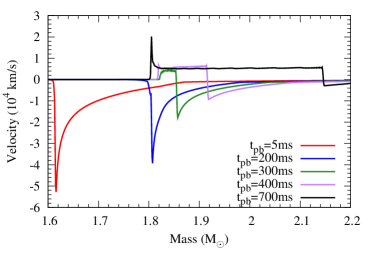
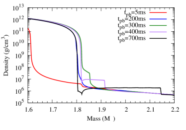
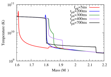
Figure 1: Time evolution of the radial velocity (top) density (middle) and temperature (bottom) as a function of mass coordinate for model WH07s20L4. Each line indicates different time from 5 ms to 700 ms after the bounce (i.e., postbounce time). The shock begins expansion at $t_{\mathrm{pb}}\sim 300$ ms.

Figure 1 presents time evolution of radial velocity, density, and temperature as a function of mass coordinate for model WH07s20L4. It is clearly shown that a stalled shock is formed at first and then once the Si/O layer ($\approx 1.82M_{\odot}$) accretes onto the shock, the shock eventually begins to propagate outward (indicated by the positive post-shock velocity) because of the rapid decrease of the ram pressure.

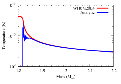
Figure 2: Maximum temperature distributions of a numerical simulation (red line) and analytic expression (blue line). Numerical model employs s20 model of Woosley & Heger (2007) and neutrino luminosity $L_{\nu}=4\times 10^{52}$ erg s^-1 and the consequent growth rate of the explosion energy is $\approx 2.2\times 10^{51}$ erg s^-1.

Figure 2 gives maximum temperature distribution as a function of mass coordinate found in model WH07s20L4 (red line) and analytic estimate based on the explosion energy (blue line). The analytic estimate is given by solving the following equation:

$$E_{\mathrm{exp}}=\frac{4\pi}{3}r_{s}^{3}aT^{4}f(T_{9}),$$ (8)

where $a=7.56\times 10^{-15}$ erg cm^-3 K^-4 is the radiation constant and $r_{s}$ is the shock radius. A temperature-dependent function $f(T_{9})=1+(7/4)T_{9}^{2}/(T_{9}^{2}+5.3)$ (Freiburghaus et al., 1999; Tominaga, 2009), which takes into account both radiation and non-degenerate electron and positron pairs, is used here. Since the temperature range is not large, $f(T_{9}=5)=2.44$ also gives a rather good agreement with numerical result. This factor makes the temperature smaller by 20% than one without the correction. In this estimate, the postshock temperature in the ejecta is assumed to be a constant in space, which is indeed realized in the simulation (see Figure 1). In the analytic estimate shown in the figure, we take the explosion energy and shock radius from the corresponding numerical simulation.

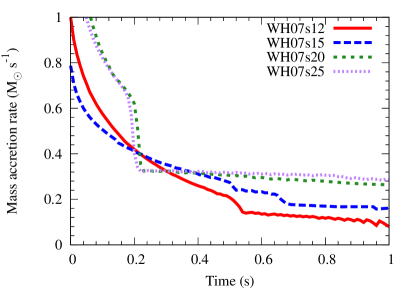
Figure 3: Mass accretion rate as a function of time after NS formation, measured at $r=500$ km. All models shown here are non-exploding models with a small neutrino luminosity.

Figure 3 presents time evolution of mass accretion rate ($\dot{M}$) of non-exploding models. Mass accretion rates are measured at $r=500$ km. Since there is a correlation between mass accretion rate and explosion criteria via critical neutrino luminosity (Burrows & Goshy, 1993), the mass accretion rate is a good measure to discuss explodability. As is known, the mass accretion rate becomes almost constant when Si/O layer is accreting (see, e.g. Suwa et al., 2016), which is seen in these simulation as well, especially in models WH07s20 and WH07s25. The constant values of accretion rate are dependent on the initial progenitor structure. From table 3, one sees that models with high $L_{\nu_{e}}$ exhibit similar explosion onset time (4th column) for WH07s20 and WH07s25, which have rapid transient in mass accretion rate (green and purple lines). Meanwhile, WH07s12 and WH07s15 do not show such a clear transition, i.e. the explosion onsets earlier for higher $L_{\nu_{e}}$, since these progenitor do not have a drastic change of mass accretion rate (red and blue lines).

3 Analytic model

In this section, we derive the temperature evolution based on a simple analytic model and justify it with numerical results explained in the previous section.

3.1 The expansion-wave collapse solution

As known in star formation field, there is a self-similar solution of stellar collapse, so-called “expansion-wave collapse solution” (Shu, 1977). This solution implies that the density structure inside rarefaction wave becomes $\rho(r)\propto r^{-3/2}$ and $r^{-2}$ outside for isothermal gas. Suto & Silk (1988) extended this solution for adiabatic flow with arbitrary adiabatic index and showed that $\rho\propto r^{-3/2}$ profile inside rarefaction wave is obtained irrespective of adiabatic index.

From modern supernova simulations, typical progenitors lead to a constant mass accretion rates when Si/O layer is accreting (see Appendix A of Suwa et al., 2016). With this fact and continuity equation, $\partial_{t}\rho+r^{-2}\partial_{r}(r^{2}\rho v)=0$, where $\partial_{t}=\partial/\partial t$ and $\partial_{r}=\partial/\partial r$, one recognizes that the density structure does not evolve, i.e. $\partial_{t}\rho=0$, since $r^{2}\rho v=\dot{M}/4\pi$ becomes constant.

The current understanding of explosion onset is the following. A rapid density decrease between Si/O layers leads to decrease of the ram pressure above the shock due to decreasing mass accretion rate. It results in a shock expansion, since the thermal pressure changes more slowly and overwhelms the ram pressure. Therefore, when the base of the oxygen layer arrives at the shock, the shock expands and, simultaneously, the density structure above shock becomes quasi-stationary. In the following we neglect time evolution of density structure above a shock wave.

3.2 Shock wave evolution

The shock velocity is given by Eq. (19) of Matzner & McKee (1999) as

$$v_{s}=0.794\left(\frac{E_{\mathrm{exp}}}{M_{\rm ej}}\right)^{1/2}\left(\frac{M_{\rm ej}}{\rho(r_{s})r_{s}^{3}}\right)^{0.19},$$ (9)

where $E_{\mathrm{exp}}$, $M_{\rm ej}$, and $r_{s}$ are explosion energy, ejecta mass, and shock radius, respectively. The ejecta mass is given by

$$M_{\rm ej}(t,r_{s})=\dot{M}t+\int_{r_{\rm mc}}^{r_{s}}4\pi r^{2}\rho(r)dr,$$ (10)

where $r_{\rm mc}$ is the radius of mass cut, i.e. the initial position of the shock. We assume the density profile as (see previous subsection)

$$\rho(r)=\rho_{R}\left(\frac{r}{R}\right)^{-3/2},$$ (11)

where $\rho_{R}$ and $R$ are constants. Adopting the mass accretion rate as $\dot{M}=4\pi r_{s}^{2}\rho(r_{s})v_{\rm acc}(r_{s})=2\pi\rho_{R}R^{3/2}\sqrt{2GM}$ ($v_{\rm acc}=v_{\mathrm{ff}}/2=\sqrt{GM/2r_{s}}$, where $v_{\mathrm{ff}}=\sqrt{2GM/r}$ is free-fall velocity, is used), we get

$$M_{\rm ej}(t,r_{s})=2\pi\rho_{R}R^{3/2}\left[\sqrt{2GM}t+\frac{4}{3}\left(r_{s}^{3/2}-r_{\rm mc}^{3/2}\right)\right].$$ (12)

Here, we also assume a constant mass accretion rate. By assuming $r_{s}=v_{s}t$ with a constant shock velocity $v_{s}$, one finds that at the early time ($t\mathrel{\hbox{\hbox to0.0pt{\hbox{\lower 5.0pt\hbox{$\sim$}}\hss}\hbox{$<$}}}GM/v_{s}^{3}=0.19\,(M/1.4M_{\odot})\,(v_{s}/10^{4}\,\mathrm{km\,s^{-1}})^{-3}$ s), a contribution from mass accretion (the first term in square bracket of Eq. 12) dominates the ejecta mass, and at the late time the swept mass contribution (the second term in bracket) dominates. In the following we evaluate shock evolutions in two extreme cases: i) ejecta mass is dominated by accreted mass and ii) ejecta mass is dominated by swept mass.

3.2.1 Accreted mass dominant case

Let us assume that $M_{\mathrm{ej}}=\dot{M}t$ by neglecting swept mass contribution (second term in the square brackets of Eq. 12). We also assume a constant growth rate of the explosion energy, $\dot{E}_{\mathrm{exp}}$, which gives $E_{\mathrm{exp}}=\dot{E}_{\mathrm{exp}}t$, for simplicity. Since $v_{s}=dr_{s}/dt$, by introducing Eq. (12) to Eq. (9), we obtain the following time evolution of the shock:

$$r_{s}(t)=\left(\frac{0.86\dot{E}_{\mathrm{exp}}^{1/2}}{\dot{M}^{0.31}\rho_{R}^{0.19}R^{0.57/2}}t^{1.19}+r_{\mathrm{mc}}^{2.57/2}\right)^{2/2.57}.$$ (13)

Here we use an initial condition that $r_{s}(t=0)=r_{\mathrm{mc}}$. The origin of time (i.e. $t=0$) is determined by the shock transition from a steady-accretion shock to an expanding shock, i.e. the onset time of the explosion. Here, we leave $\dot{M}$ as a free parameter because $v_{\mathrm{acc}}$ is not always half free-fall velocity. This is because a fluid element starts to fall down after the rarefaction waves passes it and before that it stays in hydrostatic configuration with no bulk velocity. Accretion rate based on progenitor structure will be given in Section 3.5.

3.2.2 Swept mass dominant case

Here we take into account swept mass contribution alone in Eq. (12), which is

$$M_{\mathrm{ej}}(t,r_{s})=\frac{8\pi}{3}\rho_{R}R^{3/2}(r_{s}^{3/2}-r_{\mathrm{mc}}^{3/2}).$$ (14)

Assuming $r_{s}\gg r_{\mathrm{mc}}$ and taking the leading order term of $(r_{\mathrm{mc}}/r_{s})$, we can integrate Eq. (9) as

$$\left[\frac{4}{7}-1.24\left(\frac{r_{\mathrm{mc}}}{r_{s}}\right)^{3/2}\right]r_{s}^{7/4}-0.669r_{\mathrm{mc}}^{7/4}$$

$$\,\,\,\,\,\,=0.274\rho_{R}^{-1/2}R^{-3/4}\dot{E}_{\mathrm{exp}}^{1/2}t^{3/2},$$ (15)

where we imposed an initial condition of $r=r_{\mathrm{mc}}$ for $t=0$. We can get shock evolution by solving this algebraic equation numerically.

By comparing Eq. (13) and solution of Eq. (15) with a direct integrated solution of Eq. (9), we find that, in the parameter regime we are interested in, shock evolution is well captured by these approximate solutions (i.e. Eqs. 13 and 15). For instance, with $\rho_{R}=10^{7}$ g cm^-3, $R=1000$ km, $\dot{M}=0.5M_{\odot}$ s^-1, and $\dot{E}_{\mathrm{exp}}=1$ Bethe s^-1, differences between these three solutions keep within $\sim$ 20% for $r_{s}\mathrel{\hbox{\hbox to0.0pt{\hbox{\lower 5.0pt\hbox{$\sim$}}\hss}\hbox{$<$}}}10,000$ km. Therefore, in Section 3.5 we use Eq. (13) to estimate temperature evolution, since this solution can be written in simply analytic manner.

3.3 Mass of ejecta

In the above estimates, we assumed that all shocked materials which accrete or are swept are included in ejecta mass. This assumption is not always correct, since part of them accrete onto a neutron star when postshock velocity is not outgoing. From Rankine-Hugoniot condition, we have following relation at shock frame:

$$\rho_{\mathrm{pre}}v_{\mathrm{pre}}=\rho_{\mathrm{post}}v_{\mathrm{post}},$$ (16)

where quantities with “pre” mean pre-shock states and “post” mean post-shock states. By going to rest frame, we have

$$\rho_{\mathrm{pre}}(v_{\mathrm{pre}}-v_{s})=\rho_{\mathrm{post}}(v_{\mathrm{post}}-v_{s}).$$ (17)

The preshock and postshock densities are related by $\rho_{\mathrm{post}}=\beta\rho_{\mathrm{pre}}$, where $\beta\approx 4$ (Müller et al., 2016). In order to make postshock velocity positive (i.e. $v_{\mathrm{post}}>0$), $v_{s}>-v_{\mathrm{pre}}/(\beta-1)\approx-v_{\mathrm{pre}}/3$. Note that preshock velocity is negative ($v_{\mathrm{pre}}<0$), i.e. accreting, here. It should be noted that the same constraint is obtained even when we additionally employ momentum conservation equation. By combining this requirement with Eq. (9), we can estimate the ejecta mass excluding infalling material at the onset of the explosion as follows.

$$M_{\mathrm{ej}}(t\approx 0,r_{s}) =\left[3.36(GM)^{-1/2}E_{\mathrm{exp}}^{1/2}(\rho_{R}R^{3/2})^{-0.19}r_{s}^{0.215}\right]^{1/0.31}$$ (18)

$$=0.019M_{\odot}M_{1.4}^{-1.61}E_{\mathrm{exp},49}^{1.61}\rho_{R,7}^{-0.613}R_{8}^{-0.919}r_{s,7}^{0.694},$$ (19)

where $M_{1.4}=M/1.4M_{\odot}$, $E_{\mathrm{exp},49}=E_{\mathrm{exp}}/10^{49}$ erg, $\rho_{R,7}=\rho_{R}/10^{7}$ g cm^-3, $R_{8}=R/10^{8}$ cm, and $r_{s,7}=r_{s}/10^{7}$ cm. Here we assume $|v_{\mathrm{pre}}|=\sqrt{GM/2r_{s}}$ and $\rho(r_{s})=\rho_{R}(R/r_{s})^{3/2}$. This equation implies that ejecta mass at the very beginning of the explosion ($E_{\mathrm{exp}}=10^{49}$ erg in this estimate) is negligible. For a case with a slow growth of the explosion energy, i.e. a small $\dot{E}_{\mathrm{exp}}$, ejecta mass should keep small and most of mass, which accretes onto the shock or swept by the shock, must go through the ejecta and accrete onto a central object (a neutron star or a black hole).

Note that for large $\dot{E}_{\mathrm{exp}}$ cases, a shock is rapidly accelerated and accreting and swept materials are following the shock as ejecta. Therefore, assumption employed in the previous subsection is validated.

3.4 Critical neutrino luminosity and heating rate

In this subsection, we derive a critical value of the heating rate to produce the explosion, based on discussion of a critical neutrino luminosity in the literature. Below this critical value, the shock cannot be launched.

It is well known that there is a critical neutrino luminosity to produce an explosion driven by neutrino heating mechanism. Burrows & Goshy (1993) indicated a critical neutrino luminosity as a function of mass accretion rate as $L_{\nu_{e}}\propto\dot{M}^{1/2.3}$, in which neutrino average energy was assumed to be a constant. More recently, subsequent studies updated the expression of critical neutrino luminosity by taking into account other physical parameters, e.g. neutrino average energy, PNS radius, etc. Here, we utilize Janka (2012), which gives $L_{\nu,c}(\dot{M})\propto\dot{M}^{2/5}M_{\mathrm{NS}}^{4/5}$. In the current set up, we found that the critical neutrino luminosity for s20 is $L_{\nu_{e},c}\approx 2.7\times 10^{52}$ erg s^-1, with $M_{\mathrm{NS}}\approx 1.8M_{\odot}$ (determined by $M_{s=4}$) and $\dot{M}\approx 0.3\,M_{\odot}$ s^-1. By changing parameters to $M_{\mathrm{NS}}\approx 1.5M_{\odot}$ and $\dot{M}\approx 0.15\,M_{\odot}$ s^-1, which are relevant for s12, we get $L_{\nu_{e},c}\approx 1.8\times 10^{52}$ erg s^-1. For s15, i.e. $M_{\mathrm{NS}}\approx 1.8M_{\odot}$ and $\dot{M}\approx 0.2\,M_{\odot}$ s^-1, $L_{\nu_{e},c}\approx 2.3\times 10^{52}$ erg s^-1. These values are roughly consistent with our numerical results. Since the mass accretion rate evolution is not constant in s12 and s15, the direct comparison is not very meaningful. We do not try to derive more precise estimate, because it is not the main focus of this study.

The heating rate by neutrino can be estimated with Eqs. (83) and (86) of Janka (2001) as

$$\dot{E}_{\mathrm{exp}}=\mathcal{H-C}=3.3\times 10^{50}\mathrm{erg\,s^{-1}}(2L_{\nu_{e},52})\rho_{s,9}r_{s,7}(r_{s}/r_{g})^{2},$$ (20)

where $r_{g}$ is the gain radius, which is $\approx 100$ km, and $\rho_{s,9}$ is density behind the shock in units of $10^{9}$ g cm^-3. With $\dot{M}=4\pi r^{2}\rho v$ and compression ratio $\beta=4$, $\rho_{s,9}=0.14\dot{M}_{0.3}M_{\mathrm{NS,1.8}}^{-1/2}(r_{s,7}/2)^{-3/2}$, where $\dot{M}_{0.3}=\dot{M}/0.3M_{\odot}\,\mathrm{s}^{-1}$, $M_{\mathrm{NS,1.8}}=M_{\mathrm{NS}}/1.8M_{\odot}$, which are relevant for WH07s20. $v=\sqrt{GM_{\mathrm{NS}}/2r_{s}}$ is again used. For $L_{\nu_{e},52}=4$, $r_{s,7}=2$, and $r_{s}/r_{g}=2$, we get $\dot{E}_{\mathrm{exp}}=2.7\times 10^{51}$ erg s^-1, which roughly agrees with model WH07s20L4 (see Table 2). By combining critical neutrino luminosity, we can derive a critical heating rate to produce an explosion as

$$\dot{E}_{\mathrm{exp},c}=1.9\times 10^{51}\mathrm{erg\,s^{-1}}\dot{M}_{0.3}^{7/5}M_{1.8}^{3/10}(r_{s,7}/2)^{1/2}(r_{s}/2r_{g}).$$ (21)

This is slightly larger than a consequent value of model WH07s20L3 ($\dot{E}_{\mathrm{exp}}=1.8\times 10^{51}$ erg s^-1). The inconsistency is originated from the simplification of the analytic model, which we do not discuss further.

3.5 Temperature evolution

The temperature can be estimated by

$$\frac{4\pi}{3}r_{s}^{3}aT^{4}\zeta=E_{\mathrm{int}}+\dot{E}_{\mathrm{exp}}t,$$ (22)

where $E_{\mathrm{int}}$ is the initial internal energy and $\zeta=2.44$ (see Section 2.2). Here we assume that $E_{\mathrm{int}}$ is compensating for gravitational binding energy at onset of the explosion (i.e. the explosion energy becomes positive) so that it does not appear in the expression of the explosion energy. From this equation, the temperature is written as

$$T =\left(\frac{3(E_{\mathrm{int}}+\dot{E}_{\mathrm{exp}}t)}{4\pi r_{s}^{3}a\zeta}\right)^{1/4}$$ (23)

$$=6.0\times 10^{10}\,\mathrm{K}(E_{\mathrm{int},51}+\dot{E}_{\mathrm{exp,51}}t_{0})^{1/4}r_{s,7}^{-3/4},$$ (24)

where $E_{\mathrm{int},51}=E_{\mathrm{int}}/10^{51}$ erg and $\dot{E}_{\mathrm{exp,51}}=\dot{E}_{\mathrm{exp}}/10^{51}$ erg s^-1. By combining Eqs. (13) and (24), we get

$$T= 6.0\times 10^{10}\,\mathrm{K}(E_{\mathrm{int},51}+\dot{E}_{\mathrm{exp,51}}t_{0})^{1/4}$$

$$\times\left(\frac{320\dot{E}_{\mathrm{exp,51}}^{1/2}}{\dot{M}_{0}^{0.31}\rho_{R,7}^{0.19}R_{8}^{0.57/2}}t_{0}^{1.19}+r_{\mathrm{mc,7}}^{2.57/2}\right)^{-3/5.14},$$ (25)

where $\dot{M}_{0}=\dot{M}/M_{\odot}$ s^-1.

Next, we derive $E_{\mathrm{int}}$ that dominates the temperature evolution in the early phase, from stellar structure. Since a standing accretion shock turns to a runaway phase when the thermal pressure in postshock regime becomes larger than the ram pressure in preshock regime, the time evolution of ram pressure is crucial. The preshock ram pressure can be evaluated by the free-fall model as

$$P_{\mathrm{ram}}=\rho v_{\mathrm{acc}}^{2}=\frac{\dot{M}_{s}}{4\pi r_{s}^{2}}v_{\mathrm{acc}},$$ (26)

where $M_{s}$ is a total mass enclosed by the shock and $\dot{M}_{s}$ is mass accretion rate at the shock. Here we assume that $M_{s}+\dot{M}_{s}\delta t\approx M_{s}$, where $\delta t$ is the timescale we are interested in. The mass accretion rate is (Woosley & Heger, 2012)

$$\dot{M}_{s}=\frac{dM_{s}}{dt_{\mathrm{ff}}}=\frac{2M_{s}}{t_{\mathrm{ff}}}\frac{\rho_{0}}{\bar{\rho}_{0}-\rho_{0}},$$ (27)

where $\rho_{0}$ is the density at $t=0$ and $\bar{\rho}_{0}=3M_{s}/(4\pi r_{0}^{3})$ is the mean density inside $r_{0}$ (initial radius of the mass shell). $t_{\mathrm{ff}}$ is the free-fall time, which is $t_{\mathrm{ff}}=\sqrt{3\pi/(32G\bar{\rho}_{0})}=\sqrt{\pi^{2}r_{0}^{3}/(8GM_{s})}$ (Kippenhahn & Weigert, 1990). By combining them and using $\bar{\rho}_{0}\gg\rho_{0}$, we get

$$P_{\mathrm{ram}}=\frac{4}{3\pi}\frac{GM_{s}}{r_{0}}\rho_{0}\left(\frac{r_{0}}{r_{s}}\right)^{5/2}.$$ (28)

Therefore, the internal energy of postshock regime is given by

$$e_{\mathrm{int}}=3P_{\mathrm{ram}}=\frac{4}{\pi}\frac{GM_{s}}{r_{0}}\rho_{0}\left(\frac{r_{0}}{r_{s}}\right)^{5/2}.$$ (29)

Here we assume that the pressure is dominated by radiation component, i.e. $\gamma=4/3$.

Then, $E_{\mathrm{int}}$ can be estimated as

$$E_{\mathrm{int}} =\frac{4\pi r_{s}^{3}}{3}\times 3P_{\mathrm{rad}}$$ (30)

$$=\frac{16}{3}GM_{s}\rho_{0}r_{0}^{3/2}r_{s}^{1/2}$$ (31)

$$=3.13\times 10^{49}\left(\frac{M_{s}}{1.4M_{\odot}}\right)\left(\frac{\rho_{0}}{10^{7}\,\mathrm{g\,cm^{-3}}}\right)$$

$$\,\,\times\left(\frac{r_{s}}{100\,\mathrm{km}}\right)^{1/2}\left(\frac{r_{0}}{1000\,\mathrm{km}}\right)^{3/2}\mathrm{erg}.$$ (32)

Note that this value is not an actual total internal energy included by the shock, but is a rough estimate of an initial internal energy of the ejecta which consists of a thin shell that is promptly exploding.

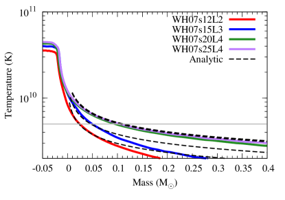
Figure 4: Maximum temperature distributions of four numerical simulations (colored solid lines) and analytic expression (black dashed lines). For analytic models, we use $\dot{E}_{\mathrm{exp}}$ taken from Table 3, $\rho$ and $R$ of $M_{s=4}+0.1M_{\odot}$ which are taken from Table 2, origin of mass coordinate set to $M_{s=4}$, and $r_{\mathrm{mc},7}=2$. $\dot{M}$ in analytic models are 0.15 (WH07s12), 0.2 (WH07s15), 0.3 (WH07s20), and 0.3 $M_{\odot}$ s^-1 (WH07s25), respectively, which are taken from Figure 3. Numerical results are horizontally sifted by $0.02M_{\odot}$ (WH07s12, WH07s20, and WH07s25) and $0.03M_{\odot}$ (WH07s15) leftward for direct comparison with analytic lines.

In Figure 4, we show a comparison between numerical results and analytic solutions for the maximum temperature distribution as a function of mass coordinate. We pick up WH07s12L2, WH07s15L3, WH07s20L4, and WH07s25L4, for typical models, since these models start exploding when the mass accretion rate is (almost) constant (see Table 3 and Figure 3). For analytic models, we solve shock evolution by Eq. (13), which only includes accreted mass in the ejecta mass, but we also add swept mass by using Eq. (11) and values ($\rho$ and $R$) at $M=M_{s=4}+0.1M_{\odot}$ from Table 2. This approximation works well, since the shock evolution by Eq. (13) is not largely different from a direct numerical integration of Eq. (9) (see Section 3.2.2). In addition, we use $\dot{E}_{\mathrm{exp}}$ taken from Table 3, origin of mass coordinate set to $M_{s=4}$, and $r_{\mathrm{mc},7}=2$. $\dot{M}$ in analytic models are 0.15 (WH07s12), 0.2 (WH07s15), 0.3 (WH07s20), and 0.3 (WH07s25), respectively, which are taken from Figure 3. Numerical results are horizontally shifted by $0.02M_{\odot}$ (WH07s12, WH07s20, and WH07s25) and $0.03M_{\odot}$ (WH07s15) leftward for direct comparison with analytic lines in Figure 4. These shifts are showing systematic error in analytic models, but these error is small enough to discuss conventional amount of ⁵⁶Ni, i.e. 0.07$M_{\odot}$ (for SN 1987A, 1993J, and 1994I). Numerical and analytic models of WH07s20L4 and WH07s25L4 agree rather well for most regime, since these models have considerably constant mass accretion rate (see Figure 3). On the other hand, WH07s12L2 and WH07s15L3 show deviation between numerical and analytic models, especially in the late time (i.e. large mass coordinate), because these models have evolving mass accretion rates that break our assumption. Nevertheless, temperature profile where we are interested in, i.e. $T_{9}>5$, are well reproduced by the analytic models.

3.6 Multidimensional effects

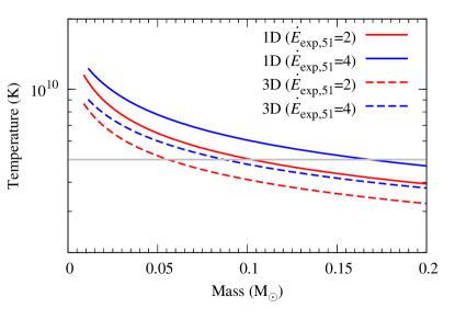
Figure 5: The same plot as Figure 4, but only analytic solutions shown for the model WH07s20. Solid and dashed lines indicate one-dimensional (1D) evolution and three-dimensional (3D) ones, respectively. Red and blue lines indicate different growth rates of the explosion energy, $\dot{E}_{\mathrm{exp}}$, respectively. A critical temperature for ⁵⁶Ni production ($T=5\times 10^{9}$ K) is also presented by grey horizontal line.

Next, let us introduce multidimensional (multi-D) effects in the analytic model. It turns out from recent neutrino-radiation hydrodynamics simulations that postshock pressure is not determined by thermal pressure alone, but turbulent pressure (i.e. Reynolds stress) is also contributing. Roughly speaking, the turbulent pressure becomes comparable to the thermal pressure (e.g. Couch & Ott, 2015). In addition, at the propagating phase the kinetic energy becomes comparable to the internal energy in the ejecta (see, e.g. Figure 14 in Bruenn et al., 2016). Therefore, it is natural to introduce a factor ($\approx 0.5$) for internal energy amount in Eqs. (25) and (32), to take into account multi-D effects, i.e.

$$E_{\mathrm{int}}+\dot{E}_{\mathrm{exp}}t\to\frac{1}{2}\left(E_{\mathrm{int}}+\dot{E}_{\mathrm{exp}}t\right).$$ (33)

Figure 5 shows the impact of multi-D effect on the temperature evolution. As is shown, the temperature of multi-D model decreases compared to one-dimensional model. We also represent the dependence of $\dot{E}_{\mathrm{exp}}$ in this figure. Roughly speaking, multi-D models produce half amount of ⁵⁶Ni of one-dimensional models, which is consistent with consequence of Yamamoto et al. (2013), in which they performed hydrodynamics simulations as well as nucleosynthesis calculations of 1D and 2D (axial symmetry).

Even below the critical heating rate derived for the 1D cases, successful explosions were observed in multi-D simulations. Multi-D effect is not only reducing the internal energy as explained above, but also reducing critical neutrino luminosity (e.g. Murphy & Burrows, 2008; Hanke et al., 2012; Couch, 2013). Previous works typically showed that multi-D simulations imply a smaller critical neutrino luminosity for the explosion than 1D ones by $\sim 20$%, depending on progenitor model. From Eq. (20), the critical $\dot{E}_{\mathrm{exp}}$ is proportional to $L_{\nu_{e}}$, the critical heating rate would be also reduced by $\sim 20$% in multi-D simulations. In addition, multi-D simulations would produce partial explosions. In particular, it is often seen in two-dimensional simulations that a part of material explodes (polar direction) and other part forms a downflow accreting onto a PNS. These structure reduces both diagnostic explosion energy and ejecta mass, and leads to smaller amount of ⁵⁶Ni. We employ the following expression to take into account partial explosion effect on the amount of ⁵⁶Ni;

$$M_{{}^{56}\mathrm{Ni}}=M_{{}^{56}\mathrm{Ni},c}\frac{\dot{E}_{\mathrm{exp}}}{\dot{E}_{\mathrm{exp,c}}},$$ (34)

where $M_{{}^{56}\mathrm{Ni},c}$ is the amount of ⁵⁶Ni corresponding to critical heating rate in multi-D model. It is worthy to note that spherical symmetric explosion maximizes the amount of ⁵⁶Ni (Maeda & Tominaga, 2009; Suwa & Tominaga, 2015).

3.7 Ejected ⁵⁶Ni mass

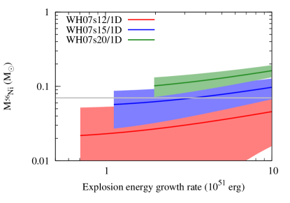
Figure 6: The amount of ⁵⁶Ni as a function of the growth rate of the explosion energy, $\dot{E}_{\mathrm{exp}}$. Horizontal grey line indicates a canonical value of ⁵⁶Ni, $0.07M_{\odot}$. Thick lines give analytic estimate with the same parameter sets as Figure 4 but different $\dot{E}_{\mathrm{exp}}$. Colored regions present possible error with $\pm 0.03M_{\odot}$, which is caused by, for instance, neutrino-driven wind upwards or fallback downward. The left endpoints correspond to the critical $\dot{E}_{\mathrm{exp}}$, which are estimated by Eq. (21). Since WH07s25 indicate rather similar result as WH07s20 (see Figure 4), it is not shown in this figure.

In this subsection, we explain the amount of ⁵⁶Ni depending on the explosion energy growth rate and progenitor models. Figure 6 presents the amount of ⁵⁶Ni as a function of $\dot{E}_{\mathrm{exp}}$ in 1D cases. All parameters other than $\dot{E}_{\mathrm{exp}}$ are the same as Figure 4. Thick lines give analytic estimate and colored region show uncertainty of models. For instance, neutrino-driven wind increases the amount of ⁵⁶Ni, definitely dependent on $Y_{e}$ profile of the wind, and fallback of ejecta conversely decreases ⁵⁶Ni. Since the impact of these effects is largely uncertain, we here roughly present error region with $\pm 0.03M_{\odot}$ as a guideline. It should be noted that this figure implies discrepancy between our numerical models and analytic model, especially for WH07s12 and WH07s15 with a rather larger $\dot{E}_{\mathrm{exp}}$ than critical value, since these models show time-evolving mass accretion rate, which breaks the assumption employed in the analytic model. The numerical models, however, employ a constant neutrino luminosity, which means feedback effects of mass accretion rate evolution are neglected. A natural expectation of the feedback effect is that the neutrino luminosity decreases as the mass accretion rate decreases. Then, shock launch is obtained once the mass accretion rate reaches a stationary state with a constant mass accretion rate, which exists for WH07s12 and WH07s15 as well, but rather late time (see Figure 3). Therefore, our analytic model works well.

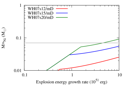
Figure 7: The same plot as Figure 6, but for multi-dimensional cases, in which reduction of thermal energy (Eq. 33), reduction of the critical heating rate (by 20% from Figure 6), and reduction of ejecta mass (Eq. 34) are taken into account. The reduction of ejecta mass is only taken into account below the critical heating rate, which makes bend of lines around $\dot{E}_{\mathrm{exp,51}}\approx 1$.

In Figure 7, we show the amount of ⁵⁶Ni by multi-D cases, in which reduction of thermal energy (Eq. 33), reduction of critical heating rate (by 20% from 1D) and reduction of ejecta mass (Eq. 34) are all taken into account. As is shown, to achieve enough ⁵⁶Ni synthesis, we need rather large growth rate of the explosion energy, larger than $\approx$4 Bethe s^-1 for WH07s20 and even larger for WH07s12 and WH07s15. Note that in this estimate, we do not include contribution from neutrino-drive wind which is largely uncertain in this study. Bruenn et al. (2016) indicated the amount of ejected ⁵⁶Ni, in which both explosive nucleosynthesis component and neutrino-driven wind component are included, as 0.035 (WH07s12), 0.077 (WH07s15), 0.065 (WH07s20), and 0.074 (WH07s20) $M_{\odot}$, respectively. The growth rate of the explosion energy is roughly, $\sim 1.5$ (WH07s12), $\sim 2$ (WH07s15), $\sim 2.5$ (WH07s20), and $\sim 3$ (WH07s25) Bethe s^-1, respectively. Therefore, by taking contributions of explosive nuclear burning from our analytic model, we find that neutrino-driven wind contributes for $\sim 0.02$ (WH07s12), $\sim 0.04$ (WH07s15), $\sim 0.01M_{\odot}$ (WH07s20 and WH07s25), respectively. It is worthy to note that their simulations in 2D exceptionally succeeded to produce enough ⁵⁶Ni, but their 3D model (Lentz et al., 2015) exhibited a much smaller $\dot{E}_{\mathrm{exp}}$ than 2D (see Table 1), which implies difficulty of ⁵⁶Ni synthesis in their 3D simulation.

4 Summary and discussion

⁵⁶Ni is an important indicator of the supernova explosion, which characterizes light curves, particularly late decay phase. In principle, the amount of ⁵⁶Ni can be directly measured by light curve alone, while ejecta mass and explosion energy are estimated by combining light curve and spectrum properties. Nevertheless, the explosion energy has often been paid attention from explosion mechanism community, since it is easier to estimate from numerical data than the amount of ⁵⁶Ni. The final explosion energy, however, is difficult to estimate by detailed numerical simulations, which solve hydrodynamics equations as well as neutrino-radiation transfer equation. This is because current simulations can reach only $\mathcal{O}(1)$ s, but the explosion energy can grow even after. On the other hand, ⁵⁶Ni should be generated within short timescale after the onset of the explosion, i.e. $\mathcal{O}(0.1)$ s, because in order to synthesize ⁵⁶Ni high temperature ($>5\times 10^{9}$ K) is necessary and temperature decreases rather fast as the shock propagates. Therefore, the amount of ⁵⁶Ni is better indicator for the explosion condition.

In this paper, we investigated the amount of ⁵⁶Ni synthesized by explosive nucleosynthesis in supernova ejecta by means of numerical simulations and an analytic model. For numerical simulations, we employ Lagrangian hydrodynamics code in which neutrino heating and cooling terms are taken into account by light-bulb approximation. Initial conditions are taken from Woosley & Heger (2007), which have 12, 15, 20, and 25 $M_{\odot}$ in zero age main sequence. We additionally developed the analytic model, which gives a reasonable estimate of the amount of ⁵⁶Ni. We found that to produce enough amount of ⁵⁶Ni (0.07 $M_{\odot}$), we need $\mathcal{O}(1)$ Bethe s^-1 of growth rate of the explosion energy, which is much larger than canonical exploding simulations, typically $\mathcal{O}(0.1)$ Bethe s^-1.

It should be noted that a recent model fitting study suggested that the distribution of $M$(⁵⁶Ni) in normal type-II supernovae is rather broad, i.e. from 0.005 to 0.28 $M_{\odot}$ (Müller et al., 2017). Our model implies that these diversity can be mainly produced by different progenitor masses, i.e. lighter progenitor models would produce less ⁵⁶Ni than more massive progenitors. However, it should be also noted that estimates of local supernovae are concentrating around 0.07 $M_{\odot}$ (e.g., Arnett et al., 1989). With precise measurements of $M$(⁵⁶Ni) and the ejecta mass (related to progenitor mass), it is able to give stringent constraint on the explosion mechanism of core-collapse supernovae. The current study also implies that in order to produce enough amount of ⁵⁶Ni, progenitor models which have a large value of compactness parameter are preferred. This is reasonable because a progenitor model, which has a small compactness parameter, is extended and temperature of important mass coordinate ($\sim 0.1M_{\odot}$ above shock launching point) cannot be high enough to synthesize ⁵⁶Ni. This trend is opposite to the explodability, which prefers a small value of compactness to produce the successful explosion. These two observations may indicate that there is a limited parameter space of progenitors, which can explain both the explodability and ⁵⁶Ni production simultaneously.

References

- Arnett (1982) Arnett W. D., 1982, ApJ, 253, 785
- Arnett et al. (1989) Arnett W. D., Bahcall J. N., Kirshner R. P., Woosley S. E., 1989, ARA&A, 27, 629
- Baade & Zwicky (1934) Baade W., Zwicky F., 1934, Proceedings of the National Academy of Science, 20, 254
- Bethe & Wilson (1985) Bethe H. A., Wilson J. R., 1985, ApJ, 295, 14
- Bruenn et al. (2013) Bruenn S. W., et al., 2013, ApJ, 767, L6
- Bruenn et al. (2016) Bruenn S. W., et al., 2016, ApJ, 818, 123
- Buras et al. (2006) Buras R., Janka H., Rampp M., Kifonidis K., 2006, A&A, 457, 281
- Burrows & Goshy (1993) Burrows A., Goshy J., 1993, ApJ, 416, L75
- Burrows et al. (2016) Burrows A., Vartanyan D., Dolence J. C., Skinner M. A., Radice D., 2016, preprint, (arXiv:1611.05859)
- Colgate & White (1966) Colgate S. A., White R. H., 1966, ApJ, 143, 626
- Couch (2013) Couch S. M., 2013, ApJ, 775, 35
- Couch & Ott (2015) Couch S. M., Ott C. D., 2015, ApJ, 799, 5
- Ertl et al. (2016) Ertl T., Janka H.-T., Woosley S. E., Sukhbold T., Ugliano M., 2016, ApJ, 818, 124
- Freiburghaus et al. (1999) Freiburghaus C., Rembges J.-F., Rauscher T., Kolbe E., Thielemann F.-K., Kratz K.-L., Pfeiffer B., Cowan J. J., 1999, ApJ, 516, 381
- Hamuy (2003) Hamuy M., 2003, ApJ, 582, 905
- Hanke et al. (2012) Hanke F., Marek A., Müller B., Janka H.-T., 2012, ApJ, 755, 138
- Höflich et al. (1999) Höflich P., Wheeler J. C., Wang L., 1999, ApJ, 521, 179
- Iwamoto et al. (1994) Iwamoto K., Nomoto K., Höflich P., Yamaoka H., Kumagai S., Shigeyama T., 1994, ApJ, 437, L115
- Janka (2001) Janka H., 2001, A&A, 368, 527
- Janka (2012) Janka H.-T., 2012, Annual Review of Nuclear and Particle Science, 62, 407
- Kippenhahn & Weigert (1990) Kippenhahn R., Weigert A., 1990, Stellar Structure and Evolution
- Lentz et al. (2015) Lentz E. J., et al., 2015, ApJ, 807, L31
- Liebendörfer et al. (2001) Liebendörfer M., Mezzacappa A., Thielemann F.-K., Messer O. E., Hix W. R., Bruenn S. W., 2001, Phys. Rev. D, 63, 103004
- Maeda & Tominaga (2009) Maeda K., Tominaga N., 2009, MNRAS, 394, 1317
- Maeda et al. (2006) Maeda K., Mazzali P. A., Nomoto K., 2006, ApJ, 645, 1331
- Marek & Janka (2009) Marek A., Janka H., 2009, ApJ, 694, 664
- Matzner & McKee (1999) Matzner C. D., McKee C. F., 1999, ApJ, 510, 379
- Melson et al. (2015) Melson T., Janka H.-T., Marek A., 2015, ApJ, 801, L24
- Mezzacappa & Bruenn (1993) Mezzacappa A., Bruenn S. W., 1993, ApJ, 405, 669
- Mihalas & Mihalas (1984) Mihalas D., Mihalas B. W., 1984, Foundations of radiation hydrodynamics
- Morozova et al. (2015) Morozova V., Piro A. L., Renzo M., Ott C. D., Clausen D., Couch S. M., Ellis J., Roberts L. F., 2015, ApJ, 814, 63
- Müller (1998) Müller E., 1998, in Steiner O., Gautschy A., eds, Saas-Fee Advanced Course 27: Computational Methods for Astrophysical Fluid Flow.. p. 343
- Müller (2015) Müller B., 2015, MNRAS, 453, 287
- Müller et al. (2012) Müller B., Janka H.-T., Marek A., 2012, ApJ, 756, 84
- Müller et al. (2016) Müller B., Heger A., Liptai D., Cameron J. B., 2016, MNRAS, 460, 742
- Müller et al. (2017) Müller T., Prieto J. L., Pejcha O., Clocchiatti A., 2017, preprint, (arXiv:1702.00416)
- Murphy & Burrows (2008) Murphy J. W., Burrows A., 2008, ApJ, 688, 1159
- Nakamura et al. (2001) Nakamura T., Mazzali P. A., Nomoto K., Iwamoto K., 2001, ApJ, 550, 991
- Nakamura et al. (2015) Nakamura K., Takiwaki T., Kuroda T., Kotake K., 2015, PASJ, 67, 107
- Nakamura et al. (2016) Nakamura K., Horiuchi S., Tanaka M., Hayama K., Takiwaki T., Kotake K., 2016, MNRAS, 461, 3296
- Nordhaus et al. (2010) Nordhaus J., Burrows A., Almgren A., Bell J., 2010, ApJ, 720, 694
- O’Connor & Couch (2015) O’Connor E., Couch S., 2015, preprint, (arXiv:1511.07443)
- O’Connor & Ott (2011) O’Connor E., Ott C. D., 2011, ApJ, 730, 70
- Pan et al. (2016) Pan K.-C., Liebendörfer M., Hempel M., Thielemann F.-K., 2016, ApJ, 817, 72
- Rampp & Janka (2000) Rampp M., Janka H., 2000, ApJ, 539, L33
- Shu (1977) Shu F. H., 1977, ApJ, 214, 488
- Smartt (2009) Smartt S. J., 2009, ARA&A, 47, 63
- Sumiyoshi et al. (2005) Sumiyoshi K., Yamada S., Suzuki H., Shen H., Chiba S., Toki H., 2005, ApJ, 629, 922
- Summa et al. (2016) Summa A., Hanke F., Janka H.-T., Melson T., Marek A., Müller B., 2016, ApJ, 825, 6
- Suto & Silk (1988) Suto Y., Silk J., 1988, ApJ, 326, 527
- Suwa & Müller (2016) Suwa Y., Müller E., 2016, MNRAS, 460, 2664
- Suwa & Tominaga (2015) Suwa Y., Tominaga N., 2015, MNRAS, 451, 4801
- Suwa et al. (2010) Suwa Y., Kotake K., Takiwaki T., Whitehouse S. C., Liebendörfer M., Sato K., 2010, PASJ, 62, L49
- Suwa et al. (2016) Suwa Y., Yamada S., Takiwaki T., Kotake K., 2016, ApJ, 816, 43
- Takiwaki et al. (2012) Takiwaki T., Kotake K., Suwa Y., 2012, ApJ, 749, 98
- Takiwaki et al. (2014) Takiwaki T., Kotake K., Suwa Y., 2014, ApJ, 786, 83
- Takiwaki et al. (2016) Takiwaki T., Kotake K., Suwa Y., 2016, MNRAS, 461, L112
- Thompson et al. (2003) Thompson T. A., Burrows A., Pinto P. A., 2003, ApJ, 592, 434
- Timmes & Arnett (1999) Timmes F. X., Arnett D., 1999, ApJS, 125, 277
- Tominaga (2009) Tominaga N., 2009, ApJ, 690, 526
- Woosley & Heger (2007) Woosley S. E., Heger A., 2007, Phys. Rep., 442, 269
- Woosley & Heger (2012) Woosley S. E., Heger A., 2012, ApJ, 752, 32
- Woosley et al. (1994) Woosley S. E., Eastman R. G., Weaver T. A., Pinto P. A., 1994, ApJ, 429, 300
- Woosley et al. (2002) Woosley S. E., Heger A., Weaver T. A., 2002, Reviews of Modern Physics, 74, 1015
- Yamamoto et al. (2013) Yamamoto Y., Fujimoto S.-i., Nagakura H., Yamada S., 2013, ApJ, 771, 27
- von Neumann & Richtmyer (1950) von Neumann J., Richtmyer R. D., 1950, Journal of Applied Physics, 21, 232