Shrinking characteristics of precision matrix estimators

Abstract

We propose a framework to shrink a user-specified characteristic of a precision matrix estimator that is needed to fit a predictive model. Estimators in our framework minimize the Gaussian negative log-likelihood plus an $L_{1}$ penalty on a linear or affine function evaluated at the optimization variable corresponding to the precision matrix. We establish convergence rate bounds for these estimators and propose an alternating direction method of multipliers algorithm for their computation. Our simulation studies show that our estimators can perform better than competitors when they are used to fit predictive models. In particular, we illustrate cases where our precision matrix estimators perform worse at estimating the population precision matrix but better at prediction.

1 Introduction

The estimation of precision matrices is required to fit many statistical models. Many papers written in the last decade have proposed shrinkage estimators of the precision matrix when the number of variables $p$ is large. Pourahmadi, (2013) and Fan et al., (2016) provide comprehensive reviews of large covariance and precision matrix estimation. The main strategy used in many of these papers is to minimize the Gaussian negative log-likelihood plus a penalty on the off-diagonal entries of the optimization variable corresponding to the precision matrix. For example, Yuan and Lin, (2007) proposed the $L_{1}$-penalized Gaussian likelihood precision matrix estimator defined by

$$\operatorname*{arg\ min}_{\Omega\in\mathbb{S}^{p}_{+}}\left\{{\rm tr}(S\Omega)-\log{\rm det}(\Omega)+\lambda\sum_{i\neq j}|\Omega_{ij}|\right\},$$ (1)

where $S$ is the sample covariance matrix, $\lambda>0$ is a tuning parameter, $\mathbb{S}^{p}_{+}$ is the set of $p\times p$ symmetric and positive definite matrices, $\Omega_{ij}$ is the $(i,j)$th entry of $\Omega$, and ${\rm tr}$ and ${\rm det}$ denote the trace and determinant, respectively. Other authors have replaced the $L_{1}$ penalty in (1) with the squared Frobenius norm (Witten and Tibshirani,, 2009; Rothman and Forzani,, 2014) or non-convex penalties that also encourage zeros in the estimator (Lam and Fan,, 2009; Fan et al.,, 2009).

To fit many predictive models, only a characteristic of the population precision matrix need be estimated. For example, in binary linear discriminant analysis, the population precision matrix is needed for prediction only through the product of the precision matrix and the difference between the two conditional distribution mean vectors. Many authors have proposed methods that directly estimate this characteristic (Cai and Liu,, 2011; Fan et al.,, 2012; Mai et al.,, 2012).

We propose to estimate the precision matrix by shrinking the characteristic of the estimator that is needed for prediction. The characteristic we consider is a linear or affine function evaluated at the precision matrix. The goal is to improve prediction performance. Unlike methods that estimate the characteristic directly, our approach provides the practitioner with an estimate of the entire precision matrix, not just the characteristic. In our simulation studies and data example, we show that penalizing the characteristic needed for prediction can improve prediction performance over competing sparse precision estimators like (1), even when the true precision matrix is very sparse. In addition, estimators in our framework can be used in applications other than linear discriminant analysis.

2 Proposed method

We propose to estimate the population precision matrix $\Omega_{*}$ with

$$\vspace{-3pt}\hat{\Omega}=\operatorname*{arg\ min}_{\Omega\in\mathbb{S}_{+}^{p}}\left\{{\rm tr}(S\Omega)-\log{\rm det}(\Omega)+\lambda|A\Omega B-C|_{1}\right\},$$ (2)

where $A\in\mathbb{R}^{a\times p}$, $B\in\mathbb{R}^{p\times b}$, and $C\in\mathbb{R}^{a\times b}$ are user-specified matrices, and $|M|_{1}=\sum_{i,j}|M_{ij}|$. Our estimator exploits the assumption that $A\Omega_{*}B-C$ is sparse. When $A$, $B$ and $C$ need to be estimated, we replace them in (2) with their estimators. The matrix $C$ can serve as a shrinkage target for $A\hat{\Omega}B$, allowing practitioners to incorporate prior information.

Dalal and Rajaratnam, (2017) proposed a class of estimators similar to (2) which replaces $A\Omega B-C$ with $T(\Omega)$, where $T$ is a symmetric linear transform.

Fitting the discriminant analysis model requires the estimation of one or more precision matrices. In particular, the linear discriminant analysis model assumes that the data are independent copies of the random pair $(X,Y)$, where the support of $Y$ is $\left\{1,\dots,J\right\}$ and

$$X\mid Y=j\sim{\rm N}_{p}\left(\mu_{*j},\Omega_{*}^{-1}\right),\quad j=1,\dots,J,$$ (3)

where $\mu_{*j}\in\mathbb{R}^{p}$ and $\Omega_{*}^{-1}\in\mathbb{S}^{p}_{+}$ are unknown. To discriminate between response categories $l$ and $m$, only the characteristic $\Omega_{*}(\mu_{*l}-\mu_{*m})$ is needed. Methods that estimate this characteristic directly have been proposed (Cai and Liu,, 2011; Mai et al.,, 2012; Fan et al.,, 2012; Mai et al.,, 2018). These methods are useful in high dimensions because they perform variable selection. For the $j$th variable to be non-informative for discriminating between response categories $l$ and $m$, it must be that the $j$th element of $\Omega_{*}(\mu_{*l}-\mu_{*m})$ is zero. While these methods can perform well in classification and variable selection, they do not actually fit the model in (3).

Methods for fitting (3) specifically for linear discriminant analysis either assume $\Omega_{*}$ is diagonal (Bickel and Levina,, 2004) or that both $\mu_{*l}-\mu_{*m}$ and $\Omega_{*}$ are sparse (Guo,, 2010; Xu et al.,, 2015). A method for fitting (3) and performing variable selection was proposed by Witten and Tibshirani, (2009). They suggest a two-step procedure where one first estimates $\Omega_{*}$, and then with the estimate $\bar{\Omega}$ fixed, estimates each $\mu_{*j}$ by penalizing the characteristic $\bar{\Omega}\mu_{j}$, where $\mu_{j}$ is the optimization variable corresponding to $\mu_{*j}.$

To apply our method to the linear discriminant analysis problem, we use (2) with $A=I_{p}$, $C$ equal to the matrix of zeros, and $B$ equal to the matrix whose columns are $\bar{x}_{j}-\bar{x}_{k}$ for all $1\leq j<k\leq J$, where $\bar{x}_{j}$ is the unpenalized maximum likelihood estimator of $\mu_{*j}$. For large values of the tuning parameter, this would lead to an estimator of $\Omega_{*}$ such that $\hat{\Omega}(\bar{x}_{j}-\bar{x}_{k})$ is sparse. Thus our approach simultaneously fits (3) and performs variable selection.

Precision and covariance matrix estimators are also needed for portfolio allocation. The optimal allocation based on the Markowitz, (1952) minimum-variance portfolio is proportional to $\Omega_{*}\mu_{*}$, where $\mu_{*}$ is the vector of expected returns for $p$ assets and $\Omega_{*}$ is precision matrix for the returns. In practice, one would estimate $\Omega_{*}$ and $\mu_{*}$ with their usual sample estimators $\hat{\Omega}$ and $\hat{\mu}$. However, when $p$ is larger than the sample size, the usual sample estimator of $\Omega_{*}$ does not exist, so regularization is necessary. Moreover, Brodie et al., (2009) argue that sparse portfolios, i.e., portfolios with fewer than $p$ active positions, are often desirable when $p$ is large. While many have proposed using sparse or shrinkage estimators of $\Omega_{*}$ or $\Omega_{*}^{-1}$ inserted in the Markowitz criterion, e.g., Xue et al., (2012), this would not necessarily lead to sparse estimators of $\Omega_{*}\mu_{*}$. To achieve a sparse portfolio, Chen et al., (2016) proposed a method for estimating the characteristic $\Omega_{*}\mu_{*}$ directly, but like the direct linear discriminant methods, it does not lead to an estimate of $\Omega_{*}$. For the sparse portfolio allocation application, we propose to estimate $\Omega_{*}$ using (2) with $A=I_{p}$, $C$ equal to the vector of zeros, and $B=\hat{\mu}$.

Another application is in linear regression where the $q$-variate response and $p$-variate predictors have a joint multivariate normal distribution. In this case, the regression coefficient matrix is $\Omega_{*}\Sigma_{*XY}$, where $\Omega_{*}$ is the marginal precision matrix for the predictors and $\Sigma_{*XY}$ is the cross-covariance matrix between predictors and response. We propose to estimate $\Omega_{*}$ using (2) with $A=I_{p}$, $C$ equal to the matrix of zeros, and $B$ equal to the usual sample estimator of $\Sigma_{*XY}.$ Similar to the proposal of Witten and Tibshirani, (2009), this approach provides an alternative method for estimating regression coefficients using shrinkage estimators of the marginal precision matrix for the predictors.

There are also applications where neither $A$ nor $B$ is equal to $I_{p}$. For example, in quadratic discriminant analysis, if one assumes that $\mu_{*j}^{\mathrm{\scriptstyle T}}\Omega_{*j}\mu_{*j}$ is small, e.g., $\mu_{*j}$ is in the span of a set of eigenvectors of $\Omega_{*j}$ corresponding to small eigenvalues, then it may be appropriate to shrink entries of the estimates of $\Omega_{j*}$, $\Omega_{*j}\mu_{*j}$, and $\mu_{*j}^{\mathrm{\scriptstyle T}}\Omega_{*j}\mu_{*j}$. For this application, we propose to estimate $\Omega_{*}$ using (2) with $C$ equal to the matrix of zeros and $A^{\mathrm{\scriptstyle T}}=B=(\bar{x}_{j},\gamma I_{p})$, for some tuning parameter $\gamma>0$.

3 Computation

3.1 Alternating direction method of multipliers algorithm

To solve the optimization in (2), we propose an alternating direction method of multipliers algorithm with a modification based on the majorize-minimize principle (Lange,, 2016). Following the standard alternating direction method of multipliers approach (Boyd et al.,, 2011), we rewrite (2) as a constrained optimization problem:

$$\operatorname*{arg\ min}_{\left(\Theta,\Omega\right)\in\mathbb{R}^{a\times b}\times\mathbb{S}^{p}_{+}}\left\{{\rm tr}(S\Omega)-\log{\rm det}(\Omega)+\lambda|\Theta|_{1}\right\}\quad\text{subject to }A\Omega B-\Theta=C.$$ (4)

The augmented Lagrangian for (4) is defined by

$$\mathcal{F}_{\rho}(\Omega,\Theta,\Gamma)={\rm tr}(S\Omega) -\log{\rm det}(\Omega)+\lambda|\Theta|_{1}$$

$$-{\rm tr}\left\{\Gamma^{\mathrm{\scriptstyle T}}(A\Omega B-\Theta-C)\right\}+\frac{\rho}{2}\|A\Omega B-\Theta-C\|_{F}^{2},$$

where $\rho>0$, $\Gamma\in\mathbb{R}^{a\times b}$ is the Lagrangian dual variable, and $\|\cdot\|_{F}$ is the Frobenius norm. Let the subscript $k$ denote the $k$th iterate. From Boyd et al., (2011), to solve (4), the alternating direction method of multipliers algorithm uses the updating equations

$$\Omega_{k+1} =\operatorname*{arg\ min}_{\Omega\in\mathbb{S}^{p}_{+}}\mathcal{F}_{\rho}(\Omega,\Theta_{k},\Gamma_{k}),$$ (5)

$$\Theta_{k+1} =\operatorname*{arg\ min}_{\Theta\in\mathbb{R}^{a\times b}}\mathcal{F}_{\rho}(\Omega_{k+1},\Theta,\Gamma_{k}),$$ (6)

$$\Gamma_{k+1} =\Gamma_{k}-\rho\left(A\Omega_{k+1}B-\Theta_{k+1}-C\right).$$ (7)

The update in (5) requires its own iterative algorithm, which is complicated by the positive definiteness of the optimization variable. To avoid this computation, we replace (5) with an approximation based on the majorize-minimize principle. In particular, we replace $\mathcal{F}_{\rho}(\cdot,\Theta_{k},\Gamma_{k})$ with a majorizing function at the current iterate $\Omega_{k}$:

$$\Omega_{k+1}=\operatorname*{arg\ min}_{\Omega\in\mathbb{S}^{+}_{p}}\left\{\mathcal{F}_{\rho}(\Omega,\Theta_{k},\Gamma_{k})+\frac{\rho}{2}{\rm vec}(\Omega-\Omega_{k})^{\mathrm{\scriptstyle T}}Q{\rm vec}(\Omega-\Omega_{k})\right\},$$ (8)

where $Q=\tau I-\left(A^{\mathrm{\scriptstyle T}}A\otimes BB^{\mathrm{\scriptstyle T}}\right),$ $\tau$ is selected so that $Q\in\mathbb{S}^{p}_{+}$, $\otimes$ is the Kronecker product, and ${\rm vec}$ forms a vector by stacking the columns of its matrix argument. Since

$${\rm vec}(\Omega-\Omega_{k})^{\mathrm{\scriptstyle T}}\left(A^{\mathrm{\scriptstyle T}}A\otimes BB^{\mathrm{\scriptstyle T}}\right){\rm vec}(\Omega-\Omega_{k})={\rm tr}\left\{A^{\mathrm{\scriptstyle T}}A(\Omega-\Omega_{k})BB^{\mathrm{\scriptstyle T}}(\Omega-\Omega_{k})\right\},$$

we can rewrite (8) as

$$\Omega_{k+1}=\operatorname*{arg\ min}_{\Omega\in\mathbb{S}^{+}_{p}}\left[\mathcal{F}_{\rho}(\Omega,\Theta_{k},\Gamma_{k})+\frac{\rho\tau}{2}\|\Omega-\Omega_{k}\|_{F}^{2}-\frac{\rho}{2}{\rm tr}\left\{A^{\mathrm{\scriptstyle T}}A(\Omega-\Omega_{k})BB^{\mathrm{\scriptstyle T}}(\Omega-\Omega_{k})\right\}\right],$$

which is equivalent to

$$\Omega_{k+1}=\operatorname*{arg\ min}_{\Omega\in\mathbb{S}^{+}_{p}}\left[{\rm tr}\left\{\left(S+G_{k}\right)\Omega\right\}-\log{\rm det}(\Omega)+\frac{\rho\tau}{2}\|\Omega-\Omega_{k}\|_{F}^{2}\right],$$ (9)

where $G_{k}=\rho A^{\mathrm{\scriptstyle T}}(A\Omega_{k}B-\rho^{-1}\Gamma_{k}-\Theta_{k}-C)B^{\mathrm{\scriptstyle T}}$. The zero gradient equation for (9) is

$$S-\Omega_{k+1}^{-1}+\frac{1}{2}\left(G_{k}+G_{k}^{\mathrm{\scriptstyle T}}\right)+\rho\tau\left(\Omega_{k+1}-\Omega_{k}\right)=0,$$ (10)

whose solution is (Witten and Tibshirani,, 2009; Price et al.,, 2015)

$$\Omega_{k+1}=\frac{1}{2\rho\tau}U\left\{-\Psi+\left(\Psi^{2}+4\rho\tau I_{p}\right)^{1/2}\right\}U^{\mathrm{\scriptstyle T}},$$

where $U\Psi U^{\mathrm{\scriptstyle T}}$ is the eigendecomposition of $S+(G_{k}+G_{k}^{\mathrm{\scriptstyle T}})/2-\rho\tau\Omega_{k}.$ Our majorize-minimize approximation is a special case of the prox-linear alternating direction method of multiplier algorithm (Chen and Teboulle,, 1994; Deng and Yin,, 2016). Using the majorize-minimize approximation of (5) guarantees that $\mathcal{F}_{\rho}(\Omega_{k+1},\Theta_{k},\Gamma_{k})\leq\mathcal{F}_{\rho}(\Omega_{k},\Theta_{k},\Gamma_{k})$ and maintains the convergence properties of our algorithm (Deng and Yin,, 2016).

Finally, (6) also has a closed form solution:

$$\Theta_{k+1}={\rm soft}\left(A\Omega_{k+1}B-\rho^{-1}\Gamma_{k}-C,\rho^{-1}\lambda\right),$$

where ${\rm soft}(x,\phi)=\max\left(|x|-\phi,0\right){\rm sign}(x)$. To summarize, we solve (2) with the following algorithm.

Algorithm 1 Alternating direction method of multipliers algorithm for (2)

Initialize $\Omega_{(0)}\in\mathbb{S}_{+}^{p}$, $\Theta_{(0)}\in\mathbb{R}^{a\times b}$, $\rho>0$, and $\tau$ such that $Q$ is positive definite. Set $k=0.$ Repeat Step 1 - 6 until convergence:

Step 1. Compute $G_{k}=\rho A^{\mathrm{\scriptstyle T}}(A\Omega_{k}B-\rho^{-1}\Gamma_{k}-\Theta_{k}-C)B^{\mathrm{\scriptstyle T}}$;

Step 2. Decompose $S+2^{-1}(G_{k}+G_{k}^{\mathrm{\scriptstyle T}})-\rho\tau\Omega_{k}=U\Psi U^{\mathrm{\scriptstyle T}}$ where $U$ is orthogonal and $\Psi$ is diagonal;

Step 3. Set $\Omega_{k+1}=(2\rho\tau)^{-1}U\left\{-\Psi+(\Psi^{2}+4\rho\tau I_{p})^{1/2}\right\}U^{\mathrm{\scriptstyle T}}$;

Step 4. Set $\Theta_{k+1}={\rm soft}(A\Omega_{k+1}B-\rho^{-1}\Gamma_{k}-C,\rho^{-1}\lambda)$;

Step 5. Set $\Gamma_{k+1}=\Gamma_{k}-\rho\left(A\Omega_{k+1}B-\Theta_{k+1}-C\right)$;

Step 6. Replace $k$ with $k+1.$

3.2 Convergence and implementation

Using the same proof technique as in Deng and Yin, (2016), one can show that the iterates from Algorithm 1 converge to their optimal values when a solution to (4) exists.

In our implementation, we set $\tau=\varphi_{1}(A^{\mathrm{\scriptstyle T}}A)\varphi_{1}(BB^{\mathrm{\scriptstyle T}})+10^{-8}$, where $\varphi_{1}(\cdot)$ denotes the largest eigenvalue of its argument. This computation is only needed once at the initialization of our algorithm. We expect that in practice, the computational complexity of our algorithm will be dominated by the eigendecomposition in Step 2, which requires $O(p^{3})$ flops.

To select the tuning parameter to use in practice, we recommend using some type of cross-validation procedure. For example, in the linear discriminant analysis case, one could select the tuning parameter that minimizes the validation misclassification rate or maximizes a validation likelihood.

4 Statistical Properties

We now show that by using the penalty in (2), we can estimate $\Omega_{*}$ and $A\Omega_{*}B$ consistently in the Frobenius and $L_{1}$ norms, respectively. We focus on the case where $C$ is the $a\times b$ matrix of zeros. A nonzero $C$ substantially complicates the theoretical analysis and is left as a direction for future research.

Our results rely on assuming that $A\Omega_{*}B$ is sparse. Define the set $\mathcal{G}$ as the indices of $A\Omega_{*}B$ that are nonzero, i.e.,

$$\mathcal{G}=\left\{(i,j)\in\left\{1,\dots,a\right\}\times\left\{1,\dots,b\right\}:\left[A\Omega_{*}B\right]_{ij}\neq 0\right\}.$$

Let the notation $[A\Omega_{*}B]_{\mathcal{G}}\in\mathbb{R}^{a\times b}$ denote the matrix whose $(i,j)$th entry is equal to the $(i,j)$th of $A\Omega_{*}B$ if $(i,j)\in\mathcal{G}$ and is equal to zero if $(i,j)\notin\mathcal{G}$. We generalize our results to the case that $A$ and $B$ are unknown, and we use plug-in estimators of them in (2).

We first establish convergence rate bounds for known $A$ and $B$. Let $\sigma_{k}(\cdot)$ and $\varphi_{k}(\cdot)$ denote the $k$th largest singular value and eigenvalue of their arguments respectively. Suppose that the sample covariance matrix used in (2) is $S_{n}=n^{-1}\sum_{i=1}^{n}X_{i}X_{i}^{\mathrm{\scriptstyle T}},$ where $X_{1},\dots,X_{n}$ are independent and identically distributed $p_{n}$-dimensional random vectors with mean zero and covariance matrix $\Omega_{*}^{-1}$. We will make the following assumptions:

Assumption 1.

For all $n$, there exists a constant $k_{1}$ such that

$$0<k_{1}^{-1}\leq\varphi_{p_{n}}(\Omega_{*})\leq\varphi_{1}(\Omega_{*})\leq k_{1}<\infty.$$

Assumption 2.

For all $n$, there exists a constant $k_{2}$ such that $\min\left\{\sigma_{p_{n}}(A),\sigma_{p_{n}}(B)\right\}\geq k_{2}>0$.

Assumption 3.

For all $n$, there exist positive constants $k_{3}$ and $k_{4}$ such that

$$\max_{j\in\left\{1,\dots,p_{n}\right\}}E\left\{{\rm exp}(tX_{1j}^{2})\right\}\leq k_{3}<\infty,\quad t\in(-k_{4},k_{4}).$$

Assumptions 1 and 3 are common in the regularized precision matrix estimation literature; Assumption 1 was made by Bickel and Levina, (2008), Rothman et al., (2008) and Lam and Fan, (2009), and Assumption 3 holds if $X_{1}$ is multivariate normal. Assumption 2 requires that $A$ and $B$ are both rank $p_{n}$, which has the effect of shrinking every entry of $\hat{\Omega}$. The convergence rate bounds we establish also depend on the quantity

$$\xi(p_{n},\mathcal{G})=\sup_{M\in\mathbb{S}^{p_{n}},M\neq 0}\frac{|\left[AMB\right]_{\mathcal{G}}|_{1}}{\|M\|_{F}},$$

where $\mathbb{S}^{p_{n}}$ is the set of symmetric $p_{n}\times p_{n}$ matrices. Negahban et al., (2012) defined a similar and more general quantity and called it a compatibility constant.

Theorem 1.

Under Assumptions 1–3, if $\lambda_{n}=K_{1}(n^{-1}\log p_{n})^{1/2}$, $K_{1}$ is sufficiently large, and $\xi^{2}(p_{n},\mathcal{G})\log p_{n}=o(n)$, then (i) $\|\hat{\Omega}-\Omega_{*}\|_{F}=O_{P}\{\xi(p_{n},\mathcal{G})(\log p_{n}/n)^{1/2}\}$ and (ii) $|A\hat{\Omega}B-A\Omega_{*}B|_{1}=O_{P}\{\xi^{2}(p_{n},\mathcal{G})(\log p_{n}/n)^{1/2}\}$.

The quantity $\xi(p_{n},\mathcal{G})$ can be used to recover known results for special cases of (2). For example, when $A$ and $B$ are identity matrices, $\xi(p_{n},\mathcal{G})={s_{n}}^{1/2}$, where $s_{n}$ is the number of nonzero entries in $\Omega_{*}$. This special case was established by Rothman et al., (2008). We can simplify the results of Theorem 1 for case that $A\Omega_{*}B$ has $g_{n}$ nonzero entries by introducing an additional assumption:

Assumption 4.

For all $n$, there exists a constant $k_{5}$ such that

$$\sup_{M\in\mathbb{S}^{p_{n}},M\neq 0}\frac{\|[AMB]_{\mathcal{G}}\|_{F}}{\|M\|_{F}}\leq k_{5}<\infty.$$

Assumption 4 is not the same as bounding $\xi(p_{n},\mathcal{G}),$ because the numerator uses the Frobenius norm instead of the $L_{1}$ norm. This requires that for those entries of $A\Omega_{*}B$ which are nonzero, the corresponding rows and columns of $A$ and $B$, do not have magnitudes too large as $p_{n}$ grows.

Corollary 1.

Under the conditions of Theorem 1 and Assumption 4, and if $A\Omega_{*}B$ has $g_{n}$ nonzero entries, then (i) $\|\hat{\Omega}-\Omega_{*}\|_{F}=O_{P}\{(g_{n}\log p_{n}/n)^{1/2}\}$ and
(ii) $|A\hat{\Omega}B-A\Omega_{*}B|_{1}=O_{P}\{(g_{n}^{2}\log p_{n}/n)^{1/2}\}.$

In practice, $A$ and $B$ are often unknown and must be estimated by $\hat{A}_{n}$ and $\hat{B}_{n}$, say. In this case, we estimate $A\Omega_{*}B$ with $\hat{A}_{n}\tilde{\Omega}\hat{B}_{n}$, where

$$\tilde{\Omega}=\operatorname*{arg\ min}_{\Omega\in\mathbb{S}_{+}^{p_{n}}}\left\{{\rm tr}(S_{n}\Omega)-\log{\rm det}(\Omega)+\lambda_{n}|\hat{A}_{n}\Omega\hat{B}_{n}|_{1}\right\}.$$ (11)

To establish convergence rate bounds for $\hat{A}_{n}\tilde{\Omega}\hat{B}_{n}$, we require an assumption on the asymptotic properties of $\hat{A}_{n}$ and $\hat{B}_{n}$:

Assumption 5.

There exist sequences $a_{n}=o(1)$ and $b_{n}=o(1)$ such that $|(A-\hat{A}_{n})A^{+}|_{1}=O_{P}\left(a_{n}\right)$ and $|B^{+}(B-\hat{B}_{n})|_{1}=O_{P}\left(b_{n}\right)$, where $A^{+}$ and $B^{+}$ are the Moore–Penrose pseudoinverses of $A$ and $B$.

The convergence rate bounds we establish for (11) also depend on the quantity $\Phi_{n}=\max(a_{n},b_{n})|\left[A\Omega_{*}B\right]_{\mathcal{G}}|_{1},$ which partly controls the additional error incurred by using estimates of $A$ and $B$ in (11).

Theorem 2.

Under Assumptions 1–3 and 5, if $\lambda_{n}=K_{2}(\log p_{n}/n)^{1/2}$, $K_{2}$ is sufficiently large, $\xi^{2}(p_{n},\mathcal{G})\log p_{n}=o(n)$, and $\Phi_{n}^{2}\log p_{n}=o(n)$, then
(i) $\|\tilde{\Omega}-\Omega\|_{F}=O_{P}\{\xi(p_{n},\mathcal{G})(\log p_{n}/n)^{1/2}+\Phi_{n}^{1/2}(\log p_{n}/n)^{1/4}\}$ and
(ii) $|\hat{A}_{n}\tilde{\Omega}\hat{B}_{n}-A\Omega_{*}B|_{1}=O_{P}\{\xi^{2}(p_{n},\mathcal{G})(\log p_{n}/n)^{1/2}+\Phi_{n}^{1/2}\xi(p_{n},\mathcal{G})(\log p_{n}/n)^{1/4}+\Phi_{n}\}.$

The convergence rate bounds in Theorem 2 are the sums of the statistical errors from Theorem 1 plus additional errors from estimating $A$ and $B$.

5 Simulation studies

5.1 Models

We compare our precision matrix estimator to competing estimators when they are used to fit the linear discriminant analysis model. For 100 independent replications, we generated a realization of $n$ independent copies of $(X,Y)$ defined in (3), where $\mu_{*j}=\Omega_{*}^{-1}\beta_{*j}$ and ${\rm pr}(Y=j)=1/J$ for $j=1,\dots,J$. Using this construction, because $\beta_{*l}-\beta_{*m}=\Omega_{*}(\mu_{*l}-\mu_{*m})$, if the $k$th element of $\beta_{*l}-\beta_{*m}$ is zero, then the $k$th variable is non-informative for discriminating between response categories $l$ and $m$.

For each $J\in\left\{3,\dots,10\right\}$, we partition our $n$ observations into a training set of size $25J$, a validation set of size $200$, and a test set of size 1000. We considered two models for $\Omega_{*}^{-1}$ and $\beta_{*j}.$ Let $\mathds{1}(\cdot)$ be the indicator function.

Model 1. We set $\beta_{*j,k}=1.5\hskip 2.0pt\mathds{1}\left[k\in\left\{4(j-1)+1,\dots,4j\right\}\right],$ so that for any pair of response categories, only eight variables were informative for discrimination. We set $\Omega^{-1}_{*a,b}=.9^{|a-b|}$, so that $\Omega_{*}$ was tridiagonal.

Model 2. We set $\beta_{*j,k}=2\hskip 2.0pt\mathds{1}\left[k\in\left\{5(j-1)+1,\dots,5j\right\}\right],$ so that for any pair of response categories, only ten variables were informative for discrimination. We set $\Omega_{*}^{-1}$ to be block diagonal: the block corresponding to the informative variables, i.e., the first $5J$ variables, had off-diagonal entries equal to 0.5 and diagonal entries equal to one. The block submatrix corresponding to the $p-5J$ non-informative variables had $(a,b)$th entry equal to $0.5^{|a-b|}.$

For both models, sparse estimators of $\Omega_{*}$ should perform well because the population precision matrices are very sparse and invertible. The total number of informative variables is $4J$ and $5J$ in Models 1 and 2 respectively, so a method like that proposed by Mai et al., (2018), which selects variables that are informative for all pairwise response category comparisons, may perform poorly when $J$ is large.

(a) Model 1 (b) Model 2

(c) Model 1 (d) Model 2

Figure 1: Misclassification rates and Frobenius norm error averaged over 100 replications with $p=200$ for Models 1 and 2. The methods displayed are the estimator we proposed in Section 2 (dashed and $\blacksquare$), the $L_{1}$-penalized Gaussian likelihood estimator (dashed and $\blacktriangle$), the Ledoit-Wolf-type estimator $\hat{\Omega}^{-1}_{\rm LW}$ (dashed and $\newmoon$), Bayes (solid and $\ast$), the method proposed by Guo, (2010) (dots and $\fullmoon$), the method proposed by Mai et al., (2018) (dots and $\triangle$), and the method proposed by Witten and Tibshirani, (2011) (dots and $\square$).

5.2 Methods

We compared several methods in terms of classification accuracy on the test set. We fit (3) using the the sparse naïve Bayes estimator proposed by Guo, (2010) with tuning parameter chosen to minimize misclassification rate on the validation set; the Bayes rule, i.e., $\Omega_{*}$, $\mu_{*j}$, and ${\rm pr}(Y=j)$ known for $j=1,\dots,J$. We also fit (3) using the ordinary sample means and using the precision matrix estimator proposed in Section 2 with tuning parameter chosen to minimize misclassification rate on the validation set and $B$ estimated using the sample means; the $L_{1}$-penalized Gaussian likelihood precision matrix estimator (Yuan and Lin,, 2007; Rothman et al.,, 2008; Friedman et al.,, 2008) with tuning parameter chosen to minimize the misclassification rate of the validation set; and a covariance matrix estimator similar to that proposed by Ledoit and Wolf, (2004), which is defined by $\hat{\Omega}^{-1}_{\rm LW}=\alpha S+\gamma(1-\alpha)I_{p},$ where $(\alpha,\gamma)\in(0,1)\times(0,\infty)$ were chosen to minimize the misclassification rate of the validation set. The $L_{1}$-penalized Gaussian likelihood precision matrix estimator we used penalized the diagonals. With our data-generating models, we found this performed better at classification than (1), which does not penalize the diagonals. We also tried two Fisher-linear-discriminant-based methods applicable to multi-category linear discriminant analysis: the sparse linear discriminant method proposed by Witten and Tibshirani, (2011) with tuning parameter and dimension chosen to minimize the misclassification rate of the validation set; and the multi-category sparse linear discriminant method proposed by Mai et al., (2018) with tuning parameter chosen to minimize the misclassification rate of the validation set.

(a) Model 1 (b) Model 2

(c) Model 1 (d) Model 2

Figure 2: True positive and true negative rates averaged over 100 replications with $p=200$ for Model 1 in (a) and (c); and for Model 2 in (b) and (d). The methods displayed are the estimator we proposed in Section 2 (dashed and $\blacksquare$), the method proposed by Guo, (2010) (dots and $\fullmoon$), and the method proposed by Mai et al., (2018) (dots and $\triangle$).

We could also have selected tuning parameters for the model-based methods by maximizing a validation likelihood or using an information criterion, but minimizing the misclassification rate on a validation set made it fairer to compare the model-based methods and the Fisher-linear-discriminant-based methods in terms of classification accuracy.

5.3 Performance measures

We measured classification accuracy on the test set for each replication for the methods described in Section 5.2. For the methods that produced a precision matrix estimator, we also measured this estimator’s Frobenius norm error: $\|\bar{\Omega}-\Omega_{*}\|_{F}$, where $\bar{\Omega}$ is the estimator. To measure variable selection accuracy, we used both the true positive rate and the true negative rate, which are respectively defined by

$$\dfrac{{\rm card}\left\{(m,k):\hat{\Delta}_{m,k}\neq 0\cap\Delta_{*m,k}\neq 0\right\}}{{\rm card}\left\{(m,k):\Delta_{*m,k}\neq 0\right\}},\quad\dfrac{{\rm card}\left\{(m,k):\hat{\Delta}_{m,k}=0\cap\Delta_{*m,k}=0\right\}}{{\rm card}\left\{(m,k):\Delta_{*m,k}=0\right\}},$$

where $(m,k)\in\left\{2,\dots,J\right\}\times\left\{1,\dots,p\right\}$, $\Delta_{*m}=\beta_{*1}-\beta_{*m}$, $\hat{\Delta}_{m}$ is an estimator of $\Delta_{*m}$, and ${\rm card}$ denotes the cardinality of a set.

5.4 Results

We display average misclassification rates and Frobenius norm error averages for both models with $p=200$ in Figure 1, and display variable selection accuracy averages in Figure 2. For both models, our method outperformed all competitors in terms of classification accuracy for all $J$, except the Bayes rule, which uses population parameter values unknown in practice. In terms of precision matrix estimation, for Model 1, our method did better than the $L_{1}$-penalized Gaussian likelihood precision matrix estimator when the sample size was small, but became worse than the $L_{1}$-penalized Gaussian likelihood precision matrix estimator as the sample size increased. For Model 2, our method was worse than the $L_{1}$-penalized Gaussian likelihood precision matrix estimator in Frobenius norm error for precision matrix estimation, but was better in terms of classification accuracy.

The precision matrix estimation results are consistent with our theory. For Model 1, as $J$ increases, the number of nonzero entries in $A\Omega_{*}B$ also increases. Our convergence rate bound for estimating $\Omega_{*}$ gets worse as the number of nonzero entries in $A\Omega_{*}B$ increases, which may explain why our estimator’s Frobenius norm error gets worse as $J$ increases. Because the sample size increases with $J$ and the number of nonzero entries in $\Omega_{*}$ is fixed for all $J$, it is expected that the $L_{1}$-penalized Gaussian likelihood estimator improves as $J$ increases. For Model 2, as $J$ increases, more entries in $\Omega_{*}$ become close to zero so the Frobenius norm error for any shrinkage estimator should decrease. However, an important point is illustrated by Model 2: although the $L_{1}$-penalized Gaussian likelihood estimator is more accurate in terms of estimating the precision matrix, our proposed estimator still performs better in terms of classification accuracy.

In terms of variable selection, our method was competitive with the methods proposed by Guo, (2010) and Mai et al., (2018). For Model 1, our method tended to have a higher average true negative rate than the method of Guo, (2010) and a lower average true positive rate than the method of Mai et al., (2018). For Model 2, all methods tended to have relatively high average true positive rates, while our method had a higher average true negative rate than the method of Mai et al., (2018). Although the method proposed by Guo, (2010) had a higher average true negative rate for Model 2 than our proposed method had, our method performed better in terms of classification accuracy.

The performance of the method proposed by Mai et al., (2018) can be partially explained by their method’s variable selection properties. Their method either includes or excludes variables for discriminating between all pairwise response category comparisons. As $J$ increases, many variables are informative for only a small number of pairwise comparisons. Their method’s low true negative rate for Model 2 suggests that it selects a large number of uninformative variables as $J$ increases.

(a) (b)

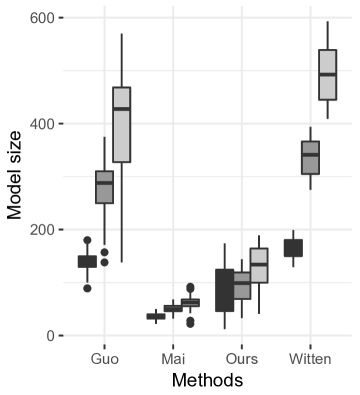
Figure 3: Model sizes and misclassification rates from 100 random training/testing splits with $k=100$ (dark grey), $k=200$ (grey), and $k=300$ (light grey). Guo is the method proposed by Guo, (2010), Mai is the method proposed by Mai et al., (2018), Glasso is the $L_{1}$-penalized Gaussian likelihood precision matrix estimator, Ours is the estimator we propose Section 2, and Witten is the method proposed by Witten and Tibshirani, (2011). Model size is the number of nonzero entries summed across the estimated discriminant vectors.

6 Genomic data example

We used our method to fit the linear discriminant analysis model in a real data application. The data are gene expression profiles consisting of $p=22,238$ genes from 127 subjects, who either have Crohn’s disease, ulcerative colitis, or neither. This dataset comes from Burczynski et al., (2006). The goal of our analysis was to fit a linear discriminant analysis model that could be used to identify which genes are informative for discriminating between each pair of the response categories. These data were also analyzed in Mai et al., (2018).

To measure the classification accuracy of our method and its competitors, we randomly split the data into training set of size 100 and test set of size 27 for 100 independent replications. Within each replication, we first applied a screening rule to the training set as in Rothman et al., (2009) and Mai et al., (2018) based on $F$-test statistics, and then restricted our discriminant analysis model to the genes with the $k$ largest $F$-test statistic values.

We chose tuning parameters with five-fold cross validation that minimized the validation classification error rate. Misclassification rates are shown in Figure 3(b), where we compared our method to those of Mai et al., (2018), of Witten and Tibshirani, (2011), of Guo, (2010), and the method that used the $L_{1}$-penalized Gaussian likelihood precision matrix estimator. Our method was at least as accurate in terms of classification as the competing methods. The only method that performed nearly as well was that of Mai et al., (2018) with $k=100$ screened genes. However, the best out-of-sample classification accuracy was achieved with $k=300,$ where our method was significantly better than the competitors.

Although the method of Mai et al., (2018) tended to estimate smaller models, our method, which performs best in classification, selects only slightly more variables. Moreover, unlike that of Mai et al., (2018), our method can be used to identify a distinct subset of genes that are informative specifically for discriminating between patients with Crohn’s disease and ulcerative colitis. This was of interest in the study of Burczynski et al., (2006). In the Supplementary Material, we provide additional details and further results.

Supplementary Material

Supplementary material available at Biometrika online includes proofs of Theorem 1 and 2; and additional information about the genomic data example.

Supplementary Material for “Shrinking characteristics of precision matrix estimators” Aaron J. Molstad¹   and Adam J. Rothman²
Biostatistics Program, Fred Hutchinson Cancer Research Center¹
School of Statistics, University of Minnesota²
amolstad@fredhutch.org¹    arothman@umn.edu²

7 Proofs

7.1 Notation

Define the following norms: $\|A\|_{\infty}=\max_{i,j}|A_{ij}|,$ $|A|_{1}=\sum_{i,j}|A_{ij}|$, and $\|A\|_{F}={\rm tr}(A^{\mathrm{\scriptstyle T}}A)$. Let $\mathbb{S}^{p_{n}}$ denote the set of $p_{n}\times p_{n}$ symmetric matrices. To simplify notation, let $\kappa=k_{1}^{-2}$.

7.2 Proof of Theorem 1

To prove Theorem 1, we use a strategy similar to that employed by Rothman, (2012).

Lemma 1.

Under Assumptions 1–3, if $\lambda_{n}\leq\epsilon\kappa\left\{\xi(p_{n},\mathcal{G})\eta_{1}\right\}^{-1}$ for some $\eta_{1}>12,$ then for all positive and sufficiently small $\epsilon$, $\|B^{+}(S_{n}-\Omega_{*}^{-1})A^{+}\|_{\infty}\leq\lambda_{n}/2$ implies $\|\hat{\Omega}-\Omega_{*}\|_{F}\leq\epsilon$ for sufficiently large $n$.

Proof.

We follow the proof techniques used by Rothman et al., (2008), Negahban et al., (2012) and Rothman, (2012). Define $B_{\epsilon}=\left\{\Delta\in\mathbb{S}^{p_{n}}:\|\Delta\|_{F}=\epsilon\right\}.$ Let $f$ be the objective function in (2). Because $f$ is convex and $\hat{\Omega}$ is its minimizer, ${\rm inf}\left\{f(\Omega_{*}+\Delta):\Delta\in B_{\epsilon}\right\}>f(\Omega_{*}),$ implies $\|\hat{\Omega}-\Omega_{*}\|_{F}\leq\epsilon$ (Rothman et al.,, 2008). Define $D(\Delta)=f(\Omega_{*}+\Delta)-f(\Omega_{*}).$ Then

$$D(\Delta)={\rm tr}(S_{n}\Delta)+\log{\rm det}(\Omega_{*})-\log{\rm det}(\Omega_{*}+\Delta)+\lambda_{n}\left\{|A(\Omega_{*}+\Delta)B|_{1}-|A\Omega_{*}B|_{1}\right\}.$$

By the arguments used in Rothman et al., (2008), $\log{\rm det}(\Omega_{*})-\log{\rm det}(\Omega_{*}+\Delta)\geq-{\rm tr}(\Omega_{*}^{-1}\Delta)+8^{-1}\kappa\|\Delta\|_{F}^{2},$ so that

$$D(\Delta)\geq{\rm tr}\left\{\Delta(S_{n}-\Omega_{*}^{-1})\right\}+\frac{1}{8}\kappa\|\Delta\|_{F}^{2}+\lambda_{n}\left\{|A(\Omega_{*}+\Delta)B|_{1}-|A\Omega_{*}B|_{1}\right\}.$$ (12)

We now bound $|A(\Omega_{*}+\Delta)B|_{1}-|A\Omega_{*}B|_{1}$ in (12). Recall that

$$\mathcal{G}=\left\{(i,j)\in\left\{1,\dots,a\right\}\times\left\{1,\dots,b\right\}:[A\Omega_{*}B]_{ij}\neq 0\right\}$$

and $\mathcal{G}^{c}=\left\{1,\dots,a\right\}\times\left\{1,\dots,b\right\}\setminus\mathcal{G}$. Since $|A\Omega_{*}B|_{1}=|\left[A\Omega_{*}B\right]_{\mathcal{G}}|_{1}$ and $|A(\Omega_{*}+\Delta)B|_{1}=|\left[A\Omega_{*}B\right]_{\mathcal{G}}+\left[A\Delta B\right]_{\mathcal{G}}|_{1}+|\left[A\Delta B\right]_{\mathcal{G}^{c}}|_{1},$ we can apply the reverse triangle inequality: $|A(\Omega_{*}+\Delta)B|_{1}-|A\Omega_{*}B|_{1}\geq|\left[A\Delta B\right]_{\mathcal{G}^{c}}|_{1}-|\left[A\Delta B\right]_{\mathcal{G}}|_{1}.$ Plugging this bound into (12),

$$D(\Delta)\geq{\rm tr}\left\{(S_{n}-\Omega_{*}^{-1})\Delta\right\}+\frac{1}{8}\kappa\|\Delta\|_{F}^{2}+\lambda_{n}\left(|\left[A\Delta B\right]_{\mathcal{G}^{c}}|_{1}-|\left[A\Delta B\right]_{\mathcal{G}}|_{1}\right).$$ (13)

We now bound ${\rm tr}\left\{(S_{n}-\Omega_{*}^{-1})\Delta\right\}$. Let $A^{+}=(A^{\mathrm{\scriptstyle T}}A)^{-1}A^{\mathrm{\scriptstyle T}}$ and $B^{+}=B^{\mathrm{\scriptstyle T}}(BB^{\mathrm{\scriptstyle T}})^{-1}$. Because $A$ and $B$ are both rank $p_{n}$ by Assumption 2, $A^{+}A=I_{p_{n}}$ and $BB^{+}=I_{p_{n}}$. Thus

$${\rm tr}\left\{(S_{n}-\Omega_{*}^{-1})\Delta\right\} \geq-|{\rm tr}\left\{(S_{n}-\Omega_{*}^{-1})\Delta\right\}|=-|{\rm tr}\left\{(S_{n}-\Omega_{*}^{-1})A^{+}A\Delta BB^{+}\right\}|$$

$$=-|{\rm tr}\left\{B^{+}(S_{n}-\Omega_{*}^{-1})A^{+}A\Delta B\right\}|$$

$$\geq-\|B^{+}(S_{n}-\Omega_{*}^{-1})A^{+}\|_{\infty}|A\Delta B|_{1}.$$ (14)

By assumption, $\|B^{+}(S_{n}-\Omega_{*}^{-1})A^{+}\|_{\infty}\leq\lambda_{n}/2$, so applying (14) to (13),

$$D(\Delta) \geq\frac{1}{8}\kappa\|\Delta\|_{F}^{2}-\frac{\lambda_{n}}{2}|A\Delta B|_{1}+\lambda_{n}\left(|\left[A\Delta B\right]_{\mathcal{G}^{c}}|_{1}-|\left[A\Delta B\right]_{\mathcal{G}}|_{1}\right)$$ (15)

$$=\frac{1}{8}\kappa\|\Delta\|_{F}^{2}-\frac{\lambda_{n}}{2}\left(|\left[A\Delta B\right]_{\mathcal{G}}|_{1}+|\left[A\Delta B\right]_{\mathcal{G}^{c}}|_{1}\right)+\lambda_{n}\left(|\left[A\Delta B\right]_{\mathcal{G}^{c}}|_{1}-|\left[A\Delta B\right]_{\mathcal{G}}|_{1}\right)$$

$$=\frac{1}{8}\kappa\|\Delta\|_{F}^{2}-\frac{3\lambda_{n}}{2}|\left[A\Delta B\right]_{\mathcal{G}}|_{1}+\frac{\lambda_{n}}{2}|\left[A\Delta B\right]_{\mathcal{G}^{c}}|_{1}$$

$$\geq\frac{1}{8}\kappa\|\Delta\|_{F}^{2}-\frac{3\lambda_{n}}{2}|\left[A\Delta B\right]_{\mathcal{G}}|_{1}.$$ (16)

Finally, we bound the quantity $|\left[A\Delta B\right]_{\mathcal{G}}|_{1}$. Multiplying and dividing $\Delta$ by $\|\Delta\|_{F}$,

$$\left|\left[A\frac{\|\Delta\|_{F}}{\|\Delta\|_{F}}\Delta B\right]_{\mathcal{G}}\right|_{1}=\|\Delta\|_{F}\left|\left[A\frac{1}{\|\Delta\|_{F}}\Delta B\right]_{\mathcal{G}}\right|_{1}\leq\|\Delta\|_{F}\left(\sup_{M\in\mathbb{S}^{p},M\neq 0}\frac{|\left[AMB\right]_{\mathcal{G}}|_{1}}{\|M\|_{F}}\right),$$

so that $|\left[A\Delta B\right]_{\mathcal{G}}|_{1}\leq\|\Delta\|_{F}\hskip 2.0pt\xi(p_{n},\mathcal{G})$. Hence, because $\|\Delta\|_{F}=\epsilon$ when $\Delta\in B_{\epsilon}$, if $\lambda_{n}\leq\epsilon\kappa\left\{\xi(p_{n},\mathcal{G})\eta_{1}\right\}^{-1}$ with $\eta_{1}>12$,

$$D(\Delta) \geq\frac{1}{8}\kappa\|\Delta\|_{F}^{2}-\frac{3\lambda_{n}}{2}\|\Delta\|_{F}\xi(p_{n},\mathcal{G})$$

$$=\|\Delta\|_{F}^{2}\left\{\frac{1}{8}\kappa-\frac{3\lambda_{n}\xi(p_{n},\mathcal{G})}{2\|\Delta\|_{F}}\right\}\geq\epsilon^{2}\left(\frac{1}{8}\kappa-\frac{3}{2\eta_{1}}\kappa\right)>0.$$

which establishes the desired result. ∎

The following lemma follows from the proof of Lemma 1 of Negahban et al., (2012).

Lemma 2.

Under the conditions of Lemma 1, $\hat{\Delta}=\hat{\Omega}-\Omega_{*}$ belongs to the set

$$\left\{\Delta\in\mathbb{S}^{p_{n}}:|\left[A\Delta B\right]_{\mathcal{G}^{c}}|_{1}\leq 3|\left[A\Delta B\right]_{\mathcal{G}}|_{1}\right\}.$$

Lemma 3 follows from the proof of Lemma 2 from Lam and Fan, (2009), Assumption 2, and Lemma A.3 of Bickel and Levina, (2008).

Lemma 3.

Under Assumptions 1–3, there exist constants $C_{1}$ and $C_{2}$ such that

$${\rm pr}(\|B^{+}S_{n}A^{+}-B^{+}\Omega_{*}^{-1}A^{+}\|_{\infty}\geq\nu)\leq C_{1}p_{n}^{2}{\rm exp}(-C_{2}n\nu^{2}),$$

for $|\nu|\leq\delta$ where $C_{1},C_{2},$ and $\delta$ do not depend on $n$.

Proof of Theorem 1.

Set $\epsilon=\kappa^{-1}\eta_{1}\xi(p_{n},\mathcal{G})K_{1}(n^{-1}\log p_{n})^{1/2}$ and $\lambda_{n}=K_{1}(n^{-1}\log p_{n})^{1/2}$ with $\eta_{1}>12$. Applying Lemma 1 and Lemma 3, there exist constants $C_{1}$ and $C_{2}$ such that for sufficiently large $n,$ ${\rm pr}\{\|\hat{\Omega}-\Omega_{*}\|_{F}\leq\kappa^{-1}\eta_{1}\xi(p_{n},\mathcal{G})K_{1}(n^{-1}\log p_{n})^{1/2}\}\geq{\rm pr}\{\|B^{+}(S_{n}-\Omega_{*}^{-1})A^{+}\|_{\infty}\leq K_{1}(n^{-1}\log p_{n})^{1/2}/2\}\geq 1-C_{1}p_{n}^{2-C_{2}K_{1}^{2}},$ which establishes $(i)$ because $1-C_{1}p_{n}^{2-C_{2}K_{1}^{2}}\to 1$ as $K_{1}\to\infty$. To establish $(ii)$,

$$|A(\hat{\Omega}-\Omega_{*})B|_{1} =|[A(\hat{\Omega}-\Omega_{*})B]_{\mathcal{G}}|_{1}+|[A(\hat{\Omega}-\Omega_{*})B]_{\mathcal{G}^{c}}|_{1}$$

$$\leq 4|[A(\hat{\Omega}-\Omega_{*})B]_{\mathcal{G}}|_{1}$$ (17)

$$\leq 4\xi(p_{n},\mathcal{G})\|\hat{\Omega}-\Omega_{*}\|_{F},$$ (18)

where (17) follows from Lemma 2 and (18) follows from the definition of $\xi(p_{n},\mathcal{G})$. ∎

7.3 Proof of Theorem 2

Lemma 4.

Let $M_{a}$ and $M_{b}$ be positive constants; and let $a_{n}$ and $b_{n}$ be positive sequences. Define $\mathcal{D}_{n}(M_{a},M_{b})$ as the event that $|(\hat{A}_{n}-A)A^{+}|_{1}\leq M_{a}a_{n}$ and $|B^{+}(\hat{B}_{n}-B)|_{1}\leq M_{b}b_{n}$. Then

$$|\hat{A}_{n}(\Omega_{*}+\Delta)\hat{B}_{n}|_{1}-|\hat{A}_{n}\Omega_{*}\hat{B}_{n}|_{1}\geq|A(\Delta+\Omega_{*})B|_{1} -|[A\Omega_{*}B]_{\mathcal{G}}|_{1}$$

$$-\tilde{M}_{n}\left(|A\Delta B|_{1}+2|[A\Omega_{*}B]_{\mathcal{G}}|_{1}\right)$$

on $\mathcal{D}_{n}(M_{a},M_{b})$, where $\tilde{M}_{n}=M_{a}a_{n}+M_{b}b_{n}+M_{a}M_{b}a_{n}b_{n}.$

Proof.

Let $|\hat{A}_{n}(\Omega_{*}+\Delta)\hat{B}_{n}|_{1}-|\hat{A}_{n}\Omega_{*}\hat{B}_{n}|_{1}\equiv V_{1}-V_{2}.$ First,

$$V_{1} =|\hat{A}_{n}(\Omega_{*}+\Delta)\hat{B}_{n}+A(\Omega_{*}+\Delta)B-A(\Omega_{*}+\Delta)B|_{1}$$

$$\geq|A(\Omega_{*}+\Delta)B|_{1}-|A(\Omega_{*}+\Delta)B-\hat{A}_{n}(\Omega_{*}+\Delta)\hat{B}_{n}|_{1},$$ (19)

by the triangle inequality. Also,

$$V_{2}=|\hat{A}_{n}\Omega_{*}\hat{B}_{n}-A\Omega_{*}B+A\Omega_{*}B|_{1}\leq|\hat{A}_{n}\Omega_{*}\hat{B}_{n}-A\Omega_{*}B|_{1}+|[A\Omega_{*}B]_{\mathcal{G}}|_{1},$$ (20)

so that from (19) and (20),

$$V_{1}-V_{2}\geq |A(\Omega_{*}+\Delta)B|_{1}-|[A\Omega_{*}B]_{\mathcal{G}}|_{1}$$

$$-|A(\Omega_{*}+\Delta)B-\hat{A}_{n}(\Omega_{*}+\Delta)\hat{B}_{n}|_{1}-|\hat{A}_{n}\Omega_{*}\hat{B}_{n}-A\Omega_{*}B|_{1}.$$ (21)

Let $$V_{3}=-|A(\Omega_{*}+\Delta)B-\hat{A}_{n}(\Omega_{*}+\Delta)\hat{B}_{n}|_{1}-|\hat{A}_{n}\Omega_{*}\hat{B}_{n}-A\Omega_{*}B|_{1} V_{3}$$. By a triangle inequality on the first term of ,

$$V_{3} \geq-2|\hat{A}_{n}\Omega_{*}\hat{B}_{n}-A\Omega_{*}B|_{1}-|\hat{A}_{n}\Delta\hat{B}_{n}-A\Delta B|_{1}.$$ (22)

To bound (22), we need to bound functions of the form $|AXB-\hat{A}_{n}X\hat{B}_{n}|_{1};$

$$|AXB-\hat{A}_{n}X\hat{B}_{n}|_{1}= |(A-\hat{A}_{n})XB+AX(B-\hat{B}_{n})+(A-\hat{A}_{n})X(\hat{B}_{n}-B)|_{1}$$

$$\leq |(A-\hat{A}_{n})XB|_{1}+|AX(B-\hat{B}_{n})|_{1}+|(A-\hat{A}_{n})X(\hat{B}_{n}-B)|_{1}.$$ (23)

$$= |(A-\hat{A}_{n})A^{+}AXB|_{1}+|AXBB^{+}(B-\hat{B}_{n})|_{1}$$

$$\hskip 104.0pt+|(A-\hat{A}_{n})A^{+}AXBB^{+}(\hat{B}_{n}-B)|_{1},$$ (24)

$$\leq |AXB|_{1}\left\{|(A-\hat{A}_{n})A^{+}|_{1}+|B^{+}(B-\hat{B}_{n})|_{1}\right.$$

$$\hskip 123.0pt\left.+|(A-\hat{A}_{n})A^{+}|_{1}|B^{+}(B-\hat{B}_{n})|_{1}\right\}$$ (25)

$$\leq |AXB|_{1}\left(M_{a}a_{n}+M_{b}b_{n}+M_{a}M_{b}a_{n}b_{n}\right),$$ (26)

where (23) follows from the triangle inequality; (24) follows from Assumption 2 and the definition of $A^{+}$ and $B^{+}$; (25) follows from the sub-multiplicative property of the $|\cdot|_{1}$ norm, and (26) occurs on $\mathcal{D}_{n}(M_{a},M_{b}).$ Applying (26) to both terms in (22) gives

$$V_{3}\geq-2|\hat{A}_{n}\Omega_{*}\hat{B}_{n}-A\Omega_{*}B|_{1}-|\hat{A}_{n}\Delta\hat{B}_{n}-A\Delta B|_{1}\geq-\tilde{M_{n}}\left(2|[A\Omega_{*}B]_{\mathcal{G}}|_{1}+|A\Delta B|_{1}\right).$$

Plugging this bound into (21) gives the result. ∎

Lemma 5.

Under Assumptions 1–3 and 5, if $n$ is sufficiently large and $\lambda_{n}\leq\epsilon\kappa(T_{\epsilon}\eta_{2})^{-1}$ for some $\eta_{2}>8$, where

$$T_{\epsilon}=\left\{\left(\frac{3}{2}+\tilde{M}_{n}\right)\xi(p_{n},\mathcal{G})+2\tilde{M}_{n}\frac{|[A\Omega_{*}B]_{\mathcal{G}}|_{1}}{\epsilon}\right\},$$

then for all positive and sufficiently small $\epsilon$, $\|B^{+}(S_{n}-\Omega_{*}^{-1})A^{+}\|_{\infty}\leq\lambda_{n}/2$, implies $\|\tilde{\Omega}-\Omega_{*}\|_{F}\leq\epsilon$.

Proof.

Let $\tilde{f}$ be the objective function from (9). Define $\tilde{D}(\Delta)=\tilde{f}(\Omega_{*}+\Delta)-\tilde{f}(\Omega_{*})$ so that

$$\tilde{D}(\Delta)={\rm tr}(S_{n}\Delta)+\log{\rm det}(\Omega_{*})-\log{\rm det}(\Omega_{*}+\Delta)+\lambda_{n}\left\{|\hat{A}_{n}(\Omega_{*}+\Delta)\hat{B}_{n}|_{1}-|\hat{A}_{n}\Omega_{*}\hat{B}_{n}|_{1}\right\}.$$

As in the proof of Lemma 1, we want to show ${\rm inf}\{\tilde{f}(\Omega_{*}+\Delta):\Delta\in B_{\epsilon}\}>\tilde{f}(\Omega_{*})$. By Assumption 5, for sufficiently large $n$, the bound in Lemma 4 holds with probability arbitrarily close to one for sufficiently large constants $M_{a}$ and $M_{b}$. Thus, let $\tilde{M}_{n}=a_{n}M_{a}+b_{n}M_{b}+a_{n}b_{n}M_{a}M_{b}$ with $M_{a}$ and $M_{b}$ sufficiently large. Then, using the bound in Lemma 4 and applying the same arguments as in the proof of Lemma 1 to obtain (15),

$$\tilde{D}(\Delta)\geq \frac{1}{8}\kappa\|\Delta\|_{F}^{2}-\frac{\lambda_{n}}{2}\left(|\left[A\Delta B\right]_{\mathcal{G}}|_{1}+|\left[A\Delta B\right]_{\mathcal{G}^{c}}|_{1}\right)+\lambda_{n}\left(|\left[A\Delta B\right]_{\mathcal{G}^{c}}|_{1}-|\left[A\Delta B\right]_{\mathcal{G}}|_{1}\right)$$

$$-\tilde{M_{n}}\lambda_{n}\left(|A\Delta B|_{1}+2|[A\Omega_{*}B]_{\mathcal{G}}|_{1}\right)$$

$$= \frac{1}{8}\kappa\|\Delta\|_{F}^{2}-\frac{3\lambda_{n}}{2}|\left[A\Delta B\right]_{\mathcal{G}}|_{1}+\frac{\lambda_{n}}{2}|[A\Delta B]_{\mathcal{G}^{c}}|_{1}-\tilde{M}_{n}\lambda_{n}\left(|A\Delta B|_{1}+2|[A\Omega_{*}B]_{\mathcal{G}}|_{1}\right)$$

$$= \frac{1}{8}\kappa\|\Delta\|_{F}^{2}-\frac{3\lambda_{n}}{2}|\left[A\Delta B\right]_{\mathcal{G}}|_{1}+\frac{\lambda_{n}}{2}|[A\Delta B]_{\mathcal{G}^{c}}|_{1}$$

$$-\tilde{M}_{n}\lambda_{n}\left(|[A\Delta B]_{\mathcal{G}}|_{1}+|[A\Delta B]_{\mathcal{G}^{c}}|_{1}+2|[A\Omega_{*}B]_{\mathcal{G}}|_{1}\right)$$

$$= \frac{1}{8}\kappa\|\Delta\|_{F}^{2}-\left(\frac{3}{2}+\tilde{M}_{n}\right)\lambda_{n}|\left[A\Delta B\right]_{\mathcal{G}}|_{1}$$

$$+\left(\frac{1}{2}-\tilde{M}_{n}\right)\lambda_{n}|[A\Delta B]_{\mathcal{G}^{c}}|_{1}-2\tilde{M}_{n}\lambda_{n}|[A\Omega_{*}B]_{\mathcal{G}}|_{1}$$ (27)

and because $\tilde{M}_{n}=o(1)$ by Assumption 5, for sufficiently large $n$, (27) implies

$$\tilde{D}(\Delta)\geq \frac{1}{8}\kappa\|\Delta\|_{F}^{2}-\left(\frac{3}{2}+\tilde{M}_{n}\right)\lambda_{n}|\left[A\Delta B\right]_{\mathcal{G}}|_{1}-2\tilde{M}_{n}\lambda_{n}|[A\Omega_{*}B]_{\mathcal{G}}|_{1}$$

$$\geq \|\Delta\|_{F}^{2}\left\{\frac{1}{8}\kappa-\left(\frac{3}{2}+\tilde{M}_{n}\right)\frac{\lambda_{n}}{\|\Delta\|_{F}}\xi(p_{n},\mathcal{G})-2\tilde{M}_{n}\lambda_{n}\frac{|[A\Omega_{*}B]_{\mathcal{G}}|_{1}}{\|\Delta\|_{F}^{2}}\right\}$$

$$= \|\Delta\|_{F}^{2}\left[\frac{1}{8}\kappa-\frac{\lambda_{n}}{\|\Delta\|_{F}}\left\{\left(\frac{3}{2}+\tilde{M}_{n}\right)\xi(p_{n},\mathcal{G})+2\tilde{M}_{n}\frac{|[A\Omega_{*}B]_{\mathcal{G}}|_{1}}{\|\Delta\|_{F}}\right\}\right].$$ (28)

Since $\|\Delta\|_{F}=\epsilon$ when $\Delta\in B_{\epsilon}$, if $\lambda_{n}\leq\epsilon\kappa(T_{\epsilon}\eta_{2})^{-1}$ for some $\eta_{2}>8$, where

$$T_{\epsilon}=\left\{\left(\frac{3}{2}+\tilde{M}_{n}\right)\xi(p_{n},\mathcal{G})+2\tilde{M}_{n}\frac{|[A\Omega_{*}B]_{\mathcal{G}}|_{1}}{\epsilon}\right\},$$

the inequality from (28) implies

$$\tilde{D}(\Delta)\geq\epsilon^{2}\left[\frac{1}{8}\kappa-\frac{\lambda_{n}}{\epsilon}\left\{\left(\frac{3}{2}+\tilde{M}_{n}\right)\xi(p_{n},\mathcal{G})+2\tilde{M}_{n}\frac{|[A\Omega_{*}B]_{\mathcal{G}}|_{1}}{\epsilon}\right\}\right]\geq\epsilon^{2}\left(\frac{1}{8}\kappa-\frac{1}{\eta_{2}}\kappa\right)>0,$$

which establishes the desired result. ∎

Lemma 6.

Under the conditions of Lemma 5, $\tilde{\Delta}=\tilde{\Omega}-\Omega_{*}$ belongs to the set

$$\left\{\Delta\in\mathbb{S}^{p_{n}}:|[A\Delta B]_{\mathcal{G}^{c}}|_{1}\leq\frac{(3+2\tilde{M}_{n})|[A\Delta B]_{\mathcal{G}}|_{1}+4\tilde{M}_{n}|[A\Omega_{*}B]_{\mathcal{G}}|_{1}}{1-2\tilde{M}_{n}}\right\}.$$

Proof.

Using the same arguments as in the proof of Lemma 1 from Negahban et al., (2012), and from (27), we have

$$0\geq\tilde{D}(\tilde{\Delta})\geq -\frac{\lambda_{n}}{2}(1+2\tilde{M}_{n})\left(|[A\tilde{\Delta}B]_{\mathcal{G}}|_{1}+|[A\tilde{\Delta}B]_{\mathcal{G}^{c}}|_{1}\right)+\lambda_{n}\left(|[A\tilde{\Delta}B]_{\mathcal{G}^{c}}|_{1}-|[A\tilde{\Delta}B]_{\mathcal{G}}|_{1}\right)$$

$$-2\lambda_{n}\tilde{M}_{n}|[A\Omega_{*}B]_{\mathcal{G}}|_{1}$$

$$= -\frac{\lambda_{n}}{2}\left\{(3+2\tilde{M}_{n})|[A\tilde{\Delta}B]_{\mathcal{G}}|_{1}-(1-2\tilde{M}_{n})|[A\tilde{\Delta}B]_{\mathcal{G}^{c}}|_{1}+4\tilde{M}_{n}|[A\Omega_{*}B]_{\mathcal{G}}|_{1}\right\}$$

so that

$$|[A\tilde{\Delta}B]_{\mathcal{G}^{c}}|_{1}\leq\frac{(3+2\tilde{M}_{n})|[A\tilde{\Delta}B]_{\mathcal{G}}|_{1}+4\tilde{M}_{n}|[A\Omega_{*}B]_{\mathcal{G}}|_{1}}{1-2\tilde{M}_{n}},$$

which is the desired inequality. ∎

Proof of Theorem 2.

Set $\lambda_{n}=K_{2}(n^{-1}\log p_{n})^{1/2}$ and $\epsilon=\lambda_{n}T_{\epsilon}\eta_{2}\kappa^{-1}$ for some $\eta_{2}>8$. We can simplify the expression for $\epsilon$ by solving

$$\epsilon\kappa\eta^{-1}_{2}(K_{2}^{2}n^{-1}\log p_{n})^{-1/2}=\left\{\left(\frac{3}{2}+\tilde{M}_{n}\right)\xi(p_{n},\mathcal{G})+2\tilde{M}_{n}\frac{|[A\Omega_{*}B]_{\mathcal{G}}|_{1}}{\epsilon}\right\},$$

or equivalently,

$$\epsilon^{2}\kappa\eta^{-1}_{2}(K_{2}^{2}n^{-1}\log p_{n})^{-1/2}-\epsilon\left(\frac{3}{2}+\tilde{M}_{n}\right)\xi(p_{n},\mathcal{G})-2\tilde{M}_{n}|[A\Omega_{*}B]_{\mathcal{G}}|_{1}=0.$$ (29)

Using the quadratic formula to solve (29) for $\epsilon$,

$$\epsilon= \frac{K_{2}\eta_{2}}{2\kappa}\left(\frac{\log p_{n}}{n}\right)^{1/2}\left[\left(\frac{3}{2}+\tilde{M}_{n}\right)\xi(p,\mathcal{G})\right.$$

$$\quad\quad\left.+\left\{\left(\frac{3}{2}+\tilde{M}_{n}\right)^{2}\xi^{2}(p_{n},\mathcal{G})+\frac{8\tilde{M}_{n}\kappa}{K_{2}\eta_{2}}\left(\frac{n}{\log p_{n}}\right)^{1/2}|[A\Omega_{*}B]_{\mathcal{G}}|_{1}\right\}^{1/2}\right].$$ (30)

To further simplify the result, we find an $\tilde{\epsilon}$ such that $\epsilon\leq\tilde{\epsilon}$. Then $\|\tilde{\Omega}-\Omega_{*}\|_{F}\leq\epsilon$ implies $\|\tilde{\Omega}-\Omega_{*}\|_{F}\leq\tilde{\epsilon}$, so $\|B^{+}(S_{n}-\Omega_{*})A^{+}\|_{\infty}\leq\lambda_{n}/2$ also implies $\|\tilde{\Omega}-\Omega_{*}\|_{F}\leq\tilde{\epsilon}$. Viewing the square root in (30) as the Euclidean norm of the sum of the square root of its two terms, we use the triangle inequality to obtain

$$\epsilon\leq\frac{K_{2}\eta_{2}}{\kappa}\left(\frac{\log p_{n}}{n}\right)^{1/2}\left[\left(\frac{3}{2}+\tilde{M}_{n}\right)\xi(p_{n},\mathcal{G})+\left\{\frac{2\tilde{M}_{n}\kappa}{K_{2}\eta_{2}}\left(\frac{n}{\log p_{n}}\right)^{1/2}|[A\Omega_{*}B]_{\mathcal{G}}|_{1}\right\}^{1/2}\right]\equiv\tilde{\epsilon}.$$

Then, applying Lemma 5 and Lemma 3, there exist constants $C_{3}$ and $C_{4}$ such that for sufficiently large $n,$

$${\rm pr}\left(\|\tilde{\Omega}-\Omega_{*}\|_{F}\leq\tilde{\epsilon}\right) \geq{\rm pr}\left\{\|B^{+}S_{n}A^{+}-B^{+}\Omega_{*}^{-1}A^{+}\|_{\infty}\leq\frac{K_{2}}{2}\left(\frac{\log p_{n}}{n}\right)^{1/2}\right\}$$

$$\geq 1-C_{3}p_{n}^{2-C_{4}K_{2}^{2}}$$

which establishes $(i)$ because $1-C_{3}p_{n}^{2-C_{4}K_{2}^{2}}\to 1$ as $K_{2}\to\infty$. To establish $(ii)$, we bound $|\hat{A}_{n}\tilde{\Omega}\hat{B}_{n}-A\Omega_{*}B|_{1}.$ By the triangle inequality,

$$|\hat{A}_{n}\tilde{\Omega}\hat{B}_{n}-A\Omega_{*}B|_{1} \leq|\hat{A}_{n}\tilde{\Omega}\hat{B}_{n}-A\tilde{\Omega}B|_{1}+|A\tilde{\Omega}B-A\Omega_{*}B|_{1}$$ (31)

and by the argument used to obtain the inequality in (26), $|\hat{A}_{n}\tilde{\Omega}\hat{B}_{n}-A\tilde{\Omega}B|_{1}\leq\tilde{M}_{n}|A\tilde{\Omega}B|_{1}.$ Using this bound on the first term in (31),

$$|\hat{A}_{n}\tilde{\Omega}\hat{B}_{n}-A\Omega_{*}B|_{1}\leq\tilde{M}_{n}|A\tilde{\Omega}B|_{1}+|A\tilde{\Omega}B-A\Omega_{*}B|_{1}.$$ (32)

Then, bounding the first term in (32), $|A\tilde{\Omega}B|_{1}\leq|A\Omega_{*}B|_{1}+|A\tilde{\Omega}B-A\Omega_{*}B|_{1}$ so that from (32),

$$|\hat{A}_{n}\tilde{\Omega}\hat{B}_{n}-A\Omega_{*}B|_{1}\leq\tilde{M}_{n}|A\Omega_{*}B|_{1}+(\tilde{M}_{n}+1)|A\tilde{\Omega}B-A\Omega_{*}B|_{1}.$$ (33)

To bound the right term in the sum on the right hand side of (33), we apply Lemma 6 to $\tilde{\Delta}=\tilde{\Omega}-\Omega_{*}$ so that

$$|A\tilde{\Omega}B-A\Omega_{*}B|_{1} =|[A\tilde{\Delta}B]_{\mathcal{G}}|_{1}+|[A\tilde{\Delta}B]_{\mathcal{G}^{c}}|_{1}$$

$$\leq|[A\tilde{\Delta}B]_{\mathcal{G}}|_{1}+\frac{(3+2\tilde{M}_{n})|[A\tilde{\Delta}B]_{\mathcal{G}}|_{1}+4\tilde{M}_{n}|[A\Omega_{*}B]_{\mathcal{G}}|_{1}}{1-2\tilde{M}_{n}}$$

$$=\frac{(1-2\tilde{M}_{n})|[A\tilde{\Delta}B]_{\mathcal{G}}|_{1}+(3+2\tilde{M}_{n})|[A\tilde{\Delta}B]_{\mathcal{G}}|_{1}+4\tilde{M}_{n}|[A\Omega_{*}B]_{\mathcal{G}}|_{1}}{1-2\tilde{M}_{n}}$$

$$=\frac{4|[A\tilde{\Delta}B]_{\mathcal{G}}|_{1}+4\tilde{M}_{n}|[A\Omega_{*}B]_{\mathcal{G}}|_{1}}{1-2\tilde{M}_{n}}.$$ (34)

Because $\tilde{M}_{n}=o(1)$ by Assumption 5, there exist constants $C_{5}$ and $C_{6}$ such that for some sufficiently large $n$, (34) implies $|A\tilde{\Omega}B-A\Omega_{*}B|_{1}\leq C_{5}\|\tilde{\Omega}-\Omega_{*}\|_{F}\xi(p_{n},\mathcal{G})+C_{6}\tilde{M}_{n}|[A\Omega_{*}B]_{\mathcal{G}}|_{1}.$ Combining this with (33),

$$|\hat{A}_{n}\tilde{\Omega}\hat{B}_{n}-A\Omega_{*}B|_{1} \leq(\tilde{M}_{n}+1)\left\{C_{5}\|\tilde{\Omega}-\Omega_{*}\|_{F}\xi(p_{n},\mathcal{G})+C_{6}\tilde{M}_{n}|[A\Omega_{*}B]_{\mathcal{G}}|_{1}\right\}+\tilde{M}_{n}|[A\Omega_{*}B]_{\mathcal{G}}|_{1}.$$

$$=C_{5}(\tilde{M}_{n}+1)\|\tilde{\Omega}-\Omega_{*}\|_{F}\xi(p_{n},\mathcal{G})+C_{6}(\tilde{M}^{2}_{n}+\tilde{M}_{n}+\tilde{M}_{n}C_{6}^{-1})|[A\Omega_{*}B]_{\mathcal{G}}|_{1}$$

and using that $\tilde{M}_{n}=o(1)$ with the result from Theorem 2 $(i)$ for $\|\tilde{\Omega}-\Omega_{*}\|_{F}$, we obtain the result. ∎

8 Additional information for the genomic data example

Figure 4: Genes selected as informative for discriminating between the subjects with ulcerative colitis (UC), subjects with Crohn’s disease, and controls. Black indicates that the variable was estimated to be informative for discriminating between the response categories. White indicates the variable was estimated to be uninformative. The leftmost three columns are based on the fitted model using our method method, whereas the MSDA column is based on the fitted model using the method of Mai et al., (2018).

The data collected by Burczynski et al., (2006) were measured on a Affymetrix HG-U133A human GeneChip array from peripheral blood mononuclear cells from 127 patients: 59 with Crohn’s disease, 26 with ulcerative colitis, and 42 controls. For our analysis, we used the log-base-2-transformed transcript measurements as predictors. These data are accessible from the Gene Expression Omnibus (https://www.ncbi.nlm.nih.gov/geo/) using accession number GDS1615. The gene names reported in Figure 4 are those that correspond to the transcripts according to the Gene Expression Omnibus database.

To compare the genes selected by the method of Mai et al., (2018) to the genes selected by our proposed method, we refit both models to the complete dataset after selecting tuning parameters to minimize the misclassification rate in five-fold cross-validation. In total, twenty-three genes were identified as informative for classification by at least one of the two methods. The method of Mai et al., (2018), which identifies variables that are informative for discriminating between all pairwise response category comparisons, identified nineteen informative genes. Our method identified twenty-one informative genes, only four of which were identified as informative for all pairwise response category comparisons.

Only six genes were selected by one method but not the other: PTGDS and PGRMC1 were selected by the method of Mai et al., (2018) but not by our method, whereas KLRF1, RBM19, NPRL2, and BASP1 were selected by our method but the method of Mai et al., (2018). Both BASP1 and RBM19 have been associated with inflammatory bowel disease, which include Crohn’s disease and ulcerative colitis, in previous studies. For example, BASP1 was identified as significantly differentially expressed between control patients and patients with inflammatory bowel disease in the study of Mesko et al., (2010). In Taleban et al., (2015), RBM19 was significantly associated with ocular extraintestinal manifestations of inflammatory bowel disease at the genome-wide level.

The majority of genes selected by our method were estimated to be important for discriminating between only two pairs of the three response categories pairwise comparisons. Thus, difference in specificity may partially explain why our method performed better than the method of Mai et al., (2018) in terms of classification accuracy. For instance, LNC2 is a known biomarker of inflammatory bowel disease (see Toyonaga et al., (2016) and references therein). Our method estimates that LNC2 is informative for discriminating subjects with Crohn’s disease from subjects with ulcerative colitis and controls, but not for discriminating between subjects with ulcerative colitis and controls. The method of Mai et al., (2018) does not allow for this distinction: their method implicitly assumes that informative genes are informative for all three response category pairwise comparisons.

Our method and the method of Mai et al., (2018) agree on certain genes associated with inflammatory bowel diseases in previous studies, e.g., SERPINB2. In the original study from Burczynski et al., (2006), the authors found that SERPINB2 was the most differentially expressed gene amongst subjects with an inflammatory bowel disease and controls.

References

- Bickel and Levina, (2004) Bickel, P. J. and Levina, E. (2004). Some theory for Fisher’s linear discriminant function, ‘naive Bayes’, and some alternatives when there are many more variables than observations. Bernoulli, 10(6):989–1010.
- Bickel and Levina, (2008) Bickel, P. J. and Levina, E. (2008). Regularized estimation of large covariance matrices. The Annals of Statistics, 36(1):199–227.
- Boyd et al., (2011) Boyd, S., Parikh, N., Chu, E., Peleato, B., and Eckstein, J. (2011). Distributed optimization and statistical learning via the alternating direction method of multipliers. Foundations and Trends in Machine Learning, 3(1):1–122.
- Brodie et al., (2009) Brodie, J., Daubechies, I., De Mol, C., Giannone, D., and Loris, I. (2009). Sparse and stable Markowitz portfolios. Proceedings of the National Academy of Sciences, 106(30):12267–12272.
- Burczynski et al., (2006) Burczynski, M. E., Peterson, R. L., Twine, N. C., Zuberek, K. A., Brodeur, B. J., Casciotti, L., Maganti, V., Reddy, P. S., Strahs, A., Immermann, F., Spinelli, W., Schertschlag, U., Slager, A. M., Cotreau, M. M., and Dorner, A. J. (2006). Molecular classification of Crohn’s disease and ulcerative colitis patients using transcriptional profiles in peripheral blood mononuclear cells. The Journal of Molecular Diagnostics, 8(1):51–61.
- Cai and Liu, (2011) Cai, T. and Liu, W. (2011). A direct estimation approach to sparse linear discriminant analysis. Journal of the American Statistical Association, 106(496):1566–1577.
- Chen and Teboulle, (1994) Chen, G. and Teboulle, M. (1994). A proximal-based decomposition method for convex minimization problems. Mathematical Programming, 64(1-3):81–101.
- Chen et al., (2016) Chen, X., Xu, M., and Wu, W. B. (2016). Regularized estimation of linear functionals of precision matrices for high-dimensional time series. IEEE Transactions on Signal Processing, 64(24):6459–6470.